Sharing Risk Under Heterogeneity: Exploring Participation Patterns in Situations of Incomplete Information

and
aInstitute of Cognitive Sciences and Technologies, National Research Council, Rome, Italy; bDepartment of Sociology, Utrecht University, Netherlands
Journal of Artificial
Societies and Social Simulation 25 (2) 5![]()
<https://www.jasss.org/25/2/5.html>
DOI: 10.18564/jasss.4789
Received: 10-Dec-2020 Accepted: 24-Feb-2022 Published: 31-Mar-2022
Abstract
Motivated by the emergence of new Peer-to-Peer insurance organizations that rethink how insurance is organized, we have proposed a theoretical model of decision-making in risk-sharing arrangements with risk heterogeneity and incomplete information about the risk distribution as core features. For these new, informal organizations, the available institutional solutions to heterogeneity (e.g., mandatory participation or price differentiation) are either impossible or undesirable. Hence, we need to understand the scope conditions under which individuals are motivated to participate in a bottom-up risk-sharing setting. The model considers participation as a utility-maximizing alternative for agents with higher risk levels, agents who are more risk averse, are driven more by solidarity motives, and less susceptible to cost fluctuations. This basic micro-level model is used to simulate decision-making for agent populations in a dynamic, interdependent setting. Simulation results show that successful risk-sharing arrangements may work if participants are driven by motivations of solidarity or risk aversion, but this is less likely in populations more heterogeneous in risk, as individual motivations can less frequently make up for larger cost deficiencies. At the same time, more heterogeneous groups deal better with uncertainty and temporary cost fluctuations than more homogeneous populations do. In the latter, cascades following temporary peaks in support requests more often result in complete failure, while under full information about the risk distribution this would not have happened.Introduction
Over the last decade, new (Peer-to-Peer) insurance organizations like Friendsurance (Germany) and Broodfonds (the Netherlands) have emerged in countries characterized by strong insurance systems. They respond to increasing privatization of social insurances, which resulted in social exclusion. In many countries welfare states do not provide social benefits to all demographic groups (e.g., excluding self-employed workers or labor migrants Baldini et al. 2016), and when insurances are offered by private insurance companies, these not rarely refuse to insure the highest risks (or ask very high insurance premiums; Natalier & Willis 2008; Taylor-Gooby 2006). To illustrate, after the Dutch welfare state abolished social benefits for self-employed workers in 2006, the latter started to self-organize in voluntary risk-sharing organizations (called Broodfonds groups) in which at most 50 people per group organize their own sickness and disability insurance (Van Leeuwen 2016). In February 2022 28,215 self-employed workers in 622 groups help each other by providing monetary support in case of sickness on the basis of solidarity and trust.
While born out of need, the organizations also seek to organize insurance differently. Inspired by mutual insurance associations (mutuals) from the 19th century, the new organizations return responsibility and trust to the policyholders by having them arrange their own safety net within small risk-sharing groups (Abdikerimova & Feng 2021).1 Risks are thus not insured top-down through a third party but are shared locally (people who participate act simultaneously in the role of the insured and the insurer), which changes the dynamics underlying participation (Jiang & Faure 2020; Liu & Faure 2018). Other than state-regulated welfare benefits, participation in these organizations is voluntary. Apart from private insurance companies, many organizations do not differentiate premium levels based on expected risk on the premise that risks cannot be assessed perfectly, and benefits should be available for everyone (Vriens & De Moor 2020).
This means that the default solutions to prevent adverse selection (i.e., the tendency to attract mainly high-risk people Arrow 1984) do not apply and begs the question why and when people are willing to share risk. If mandatory solidarity is impossible and price differentiation undesirable, how can risk-sharing groups be created that remain stable in the long term? Long-term stability is not guaranteed, because the participation costs in risk-sharing groups fluctuate depending on how many or how often group members request support. When more is saved through contributions than is needed to support members in need, (a share of) the fund’s reserves are redistributed (Breer & Novikov 2015). Thus, the lower the number of support requests, the lower the costs for everyone. Yet, participation is costly if many request support simultaneously. This introduces an interdependency where one person’s actions (support requests) directly affect the costs for others. Assuming that costs drive willingness to participate, the latter should also vary over time, thus making risk-sharing groups more fragile. Members initially interested in participating could at any time revoke their membership (e.g., because more support is requested than expected Platteau 1997), and if they do so, they take from the common fund the share of their contributions not spent on insurance benefits.
With this in mind, we need a better understanding of why people participate in voluntary risk-sharing groups without risk differentiation and when participation can be resilient to cost fluctuations. While many scholars have developed and refined (informal) risk-sharing models (Coate & Ravallion 1993; Genicot & Ray 2003; Kimball 1988; Ligon et al. 2002), these models generally assume homogeneous risk probabilities. If they do introduce heterogeneity, formal models assume complete information about the risk distribution: Rational agents base their own membership on a comparison between one’s own risk and that of other participants. Heterogeneity then introduces adverse selection (Arrow 1984). Those with the lowest risk profiles will opt out of the arrangement, followed by the second-lowest risk profiles, and so on—until either the entire risk-sharing arrangement fails or only high risks remain. However, these risk comparisons are very constraining in terms of agents’ cognitive abilities. Furthermore, it is unrealistic that agents have such detailed information about all other agents in advance. Finally, this situation comes with the hidden assumption that agents are not affected by realized outcomes (people requesting support), which is unlikely to hold in practice.
Luckily, complete information is not a requirement. As long as people assume risks to be broadly similar, risk-sharing arrangements can still arise (Skogh & Wu 2005). We propose a dynamic agent-based model where agents know their own risk2 but not the risk distribution. They base their decisions on an estimate of the group-level average. This estimate is updated every time group members do or do not request support. This approach combines forward-looking decision-making with backward-looking learning as a tool to deal with decisions under uncertainty. It implies that as more support is requested in some rounds than in others, the average risk estimate, and therefore the expected utility of participating, also fluctuates. Hence, where a complete information model has a stable equilibrium, the alternative model continues to update. On the plus side, it may lead to more people joining initially (and thus preventing failure from the start). On the downside, it increases the possibility of withdrawal cascades, where agents follow each other in withdrawing from the risk-sharing group while they may not have, had they known the true distribution.
What are the implications of this alternative approach for the effect of risk heterogeneity? The aims of this article are to investigate theoretically (1) the extent to which heterogeneous risk-sharing groups may succeed when agents do not have complete information; (2) whether the reliance on realized support requests increases the chances of generating withdrawal cascades; and (3) what alternative individual factors (risk aversion, solidarity, and reinforcement learning) are needed to obtain a safe bandwidth that enables stable participation rates despite cost fluctuations. We introduced these additional individual factors, for otherwise participation cannot be explained for everyone whose personal risk is smaller than the (estimated) group average (Coate & Ravallion 1993; Vogt & Weesie 2004).
Risk aversion reflects a preference for certain outcomes over risky situations in which outcomes are uncertain. It is deemed crucial for understanding why (low-risk) people take out insurances (Arrow 1984), but also for participation in (heterogeneous) risk-sharing groups and helping arrangements (Platteau et al. 2017; Vogt & Weesie 2004). Risk averse people participate even under low risk. Solidarity implies prosocial behavior towards members of the same group (Baldassarri 2015) from which personal utility is derived (Gintis et al. 2005). The risk-sharing groups introduce many-to-many relationships that are argued to invoke solidarity, which makes people willing to (unconditionally) pay for the insurance of other group members.3 Reinforcement learning (Macy & Flache 2002), finally, is used to explain how people let current experiences influence (or override) their previous estimate about the group’s average risk. Those who do so to a larger extent are more susceptible to cost fluctuations and therefore more likely to withdraw when costs unexpectedly (temporarily) increase.
Model Construction
We defined risk-sharing as a social dilemma under uncertainty. The creation of a common insurance fund is a collective effort, so rather than principal-agent insurance models that predict how principals offer the insurance to heterogeneous policyholders (see, e.g., Sellgren 2001 for a learning model in a heterogeneous insurance market), we took a bottom-up approach with agents acting both as the insurer and the insured (Jiang & Faure 2020) and ask when they are willing to contribute to the common fund to receive the benefit (support) in times of need. There may be a long delay between contributing to the common fund and actually obtaining the benefit of cooperation. In fact, since losses are undesirable even if they are (partially) covered, ideally one never actually needs the support from the group (Platteau 1997). Hence, the short-term benefit of withdrawing to avoid the costs of helping others may easily outweigh the uncertainty surrounding the long-term benefit of perhaps needing and receiving the security oneself someday (Fafchamps 1992). One-time individually rational decisions to withdraw (e.g., because of a sudden increase in support requests) may then translate into a collectively worse outcome where no one is insured (Coate & Ravallion 1993). Hence, participation is uncertain not only because it is unknown whether one, as an individual, ever needs a payout from the collective fund. It also derives from not knowing how many others (simultaneously) need support and under what circumstances they remain a member to pay the costs to support others (Vriens et al. 2021).
The first models on risk-sharing as a social dilemma were formalized by Kimball (1988) and Coate & Ravallion (1993). They formulated conditions under which self-interested agents enter informal risk-sharing arrangements voluntarily ex ante without defecting ex post, where ex post defection means that agents refuse to share their payoff if they end up with the higher one. The models start from a homogeneous risk assumption: Each agent is equally likely to end up with a high or low income. For an infinitely repeated game, the theoretical optimum entails full income pooling and equally sharing the aggregate available resources each period. As long as the gain from defection is small, this can be achieved regardless of group size. Empirical tests refuted this prediction, observing small groups, partial risk-sharing, and less than full insurance instead (Fafchamps & Lund 2003; Murgai et al. 2002; Townsend 1994). Hence, alternative models predict cooperation when participation only requires limited commitment (Ligon et al. 2002), when cooperation should be robust also to deviations by subgroups (Genicot & Ray 2003), when arrangements are made in networks (Bloch et al. 2008), or when participation can take place through threshold models (i.e., not all agents have to join in round 1 Breer & Novikov 2015).
Another explanation for the lack of full insurance in large groups—and the one central in this model—is the heterogeneity of the risk distribution. Formal models that start from risk heterogeneity (Attanasio et al. 2012; Hegselmann 1994; Lin et al. 2019; Skogh & Wu 2005; Vogt & Weesie 2004) predicted an optimal support relation under homogeneity, but showed that cooperation is likewise possible under heterogeneity in needing support as long as other factors may compensate for this difference. Apart from institutional features (like mandatory participation or lower contribution levels for low-risk agents), risk aversion is most often included as an individual motivation to explain participation despite low risk levels (Vogt & Weesie 2004). Operationalized using a concave utility function, risk averse agents are willing to incur larger insurance costs today to ascertain an income in the future (Arrow 1984). These dynamics have been corroborated in lab experiments. While Tausch et al. (2014) found adverse selection in risk-sharing experiments with heterogeneity in risk levels, Vogt & Weesie (2006) found that this can be compensated for by risk aversion. Simulation studies that extend this model to \(N\)-person settings predict that when players endogenously choose with whom to engage in dyadic support relations, stable support relations arise under heterogeneity in needing support as long as heterogeneity is modest and risk probabilities are average (Hegselmann & Flache 1998).
For risk-sharing settings, however, some scholars have questioned the validity of the risk aversion assumption, primarily due to the low participation rates observed in field studies (see Platteau et al. 2017 for a review). They argue that risk-sharing arrangements might not sufficiently solve the uncertainty problem. While for a formal insurance, a risk averse person chooses to pay more to be certain of not losing everything, in a risk-sharing group participation does not guarantee support. Others may withdraw or there may not be enough money available in the common insurance fund to cover everyone’s needs. Hence, participating and not participating are both uncertain strategies. Following this line of reasoning, some models (e.g., Dercon et al. 2014) have posed additional assumptions of prudence and temperance, which help selection of the most preferred alternative in situations when there is more than one source of uncertainty. While such extensions could be included at a later stage, given the large number of parameters our basic model uses plain risk aversion following a concave utility function (Kimball 1993).
Secondly, individuals often act out of some sort of other-regarding preferences (Chaudhuri 2011; Fehr & Gächter 2002; Ostrom 1990). A popular operationalization of other-regarding preferences is through models of inequity aversion (Bolton & Ockenfels 2000; Fehr & Schmidt 1999), which assume that an agent is altruistic towards others if their material payoff falls below an equitable benchmark, but feels envy when their payoffs exceed this benchmark. We label our social preferences ‘solidarity’ and assume that solidarity is triggered when other participants in the risk-sharing group are in need of support. In that sense, it resembles a simplified (one-sided) version of inequity aversion, disregarding envy and resembling models of guilt aversion (Snijders 1996; applied to risk-sharing in Lin et al. 2019). Like in Fehr & Schmidt (1999), it is implemented additively, such that solidarity makes agents willing to suffer certain costs (i.e., have smaller shares redistributed from the common fund) to cover the loss of others.
This implementation distinguishes within-group solidarity from general altruism (see also Baldassarri 2015) and enables model applications where solidarity dynamically increases or decreases depending on in-group developments (e.g., changes in the number or distribution of support requests) and relations to other group members. It is often argued that when solidarity is costly, there is a decay in the salience of solidarity motivations over time. Especially for repeated solidarity, the feedback of the recipient (in terms of approval) tends to be more intermittent than the costs to execute it (Lindenberg 1998). On the other hand, if relationships across members tighten over time and groups become more cohesive, solidarity may also increase (Vriens et al. 2021). We start with a basic (static) definition of solidarity, but will—to illustrate how the model parameters may be extended to particular contexts—perform sensitivity checks to show what happens to membership rates and the success of risk-sharing arrangements when solidarity depends on the number of support requests. That is, in an alternative model solidarity motivations decrease when the estimated difference between one’s own risk and that of the group increases. Simulation models of dyadic support relations have shown, for instance, that support relations may arise even when people differ in their need for support, but that support relations are stronger when differences in need levels are smaller (Bianchi et al. 2020; Flache & Hegselmann 1999).
Finally, we implemented learning to the model so that agents agents do not know the risk levels of all group members, but update their estimate of the group’s average risk over time following new support requests by group members (or the lack thereof). In doing so, we assume bounded, backward-looking rationality (Camerer 1998). This makes deriving predictions easier and poses fewer constraints on the agents’ cognitive capabilities (Macy & Flache 2002). With reinforcement learning (Bush & Mosteller 1955), agents follow a simple updating rule. Each round, they update by some weight their estimate of a strategy’s profitability (here: of participating) based on realized payoffs in the previous round (here: driven by support requests). Hence, when more agents request support, the average risk estimate is revised upwards. The alternative, Bayesian learning, has agents consider every possible collection of agent characteristics (here: of risk distributions). Each collection receives a weight, and over time these weights are updated based on realized outcomes (Jordan 1991). Since we have an infinite number of possible risk distributions, Bayesian learning is too demanding. We therefore started from a simple model of reinforcement learning (cf. Macy & Flache 2002), where by some weight agents let current experiences (i.e., support requests) override previous estimates.
Formal model
We defined an N-person Risk-Sharing Model (RSM) in which \(N\geq2\) agents indexed by \(i \in \{1,\ldots,N \}\) choose simultaneously to become a member \((m=1)\) or not \((m=0)\) at time \(\tau=0\). At each time point \(\tau\geq1\), agents that joined decide whether or not to stay. If at any time point \(\tau\) an agent withdraws this decision is irrevocable. In each round \(\tau\geq1\), a random draw by Nature determines realized events (i.e., which agents, if any, need support) and resulting payoffs. \(n\) denotes the number of agents that are part of the Risk-Sharing Group (RSG), with \(0\leq n \leq N\). A boundedly rational, utility maximizing agent joins the RSG as long as the short-term expected payoff under \((m=1)\) exceeds that of \((m=0)\).
Each agent receives income \(Y_i\) with probability \((1-p_i)\) and \(y_i\) with probability \(p_i\), where \(Y_i-y_i\) represents the loss that can be insured (reflecting, e.g., failed harvests, a broken product, stolen goods, or poor health) and \(p_i\) is an independent and identically distributed (i.i.d.) risk probability. If agents join the RSG, they pay contribution \(c_i\) for membership and receive benefit \(b_i\) under \(p_i\), where \(c_i<b_i\) and \(y_i+b_i\leq Y_i\). For simplicity, we assume homogeneous incomes, losses, contributions, and benefits (\(Y_i=Y\), \(y_i=y\), \(c_i=c\), and \(b_i=b\)) and leave heterogeneity only with respect to \(p_i\).
To represent a collective non-profit fund, the pooled contributions that were not needed to pay benefits get redistributed among all agents with an individual share \(\delta\). That is, the expected profit on the level of the mutual corresponds to4
| \[\begin{aligned} P = \sum\limits_{i = 1}^{n} (c-p_i b-\delta)=0.\end{aligned}\] | \[(1)\] |
Bounded rationality implies that players cannot foresee the risk probabilities of other agents \(j\). Instead, we assumed that agents know their own risk \(p_i\)5 but make an estimate \(\hat{p}_i\) of the average risk probability of all other agents. \(\hat{p}_i\) is based on an intuition about the population’s risk probability and is updated over time after observing the number of support requests. We denoted for each agent \(i\) the number of other group members \(j\neq i\) that needed support as \(k_i^{\tau}\), where \(k_i^{\tau}\) influences the agent’s average risk estimate \(\hat{p}_i\) with some weight as determined by the learning parameter \(0<\omega\leq 1\), i.e.
| \[\begin{aligned} \hat{p}_i^{\tau} = (1-\omega)\hat{p}_i^{\tau-1} + \omega \frac{k_i^{\tau}}{n^{\tau}}.\end{aligned}\] | \[(2)\] |
Thus, the average risk estimate at time \(\tau\) is a function of the previous estimate and the proportion of members that requested support \(k_i/n\). Combining Equation 1 and Equation 2, the expected redistribution \(\hat{\delta}_i\) boils down to
| \[\begin{aligned} \hat{\delta}_i = \frac{n c - p_i b - \hat{p}_i (n-1) b}{n} = c - \hat{p}_i b - \frac{(\hat{p}_i-p_i)b}{n}.\end{aligned}\] | \[(3)\] |
In this equation, \(nc\) reflects the maximum available amount for redistribution. This means, on an individual level, that if no one needs support everyone gets their contribution \(c\) to the common fund returned. \(\hat{p}_i b\) reflects the estimated average loss on payments to other players, and the difference \((\hat{p}_i-p_i)\) either decreases or increases this share spent on payments depending on whether player \(i\)’s risk is lower or higher than the estimated other players’ average risk \(\hat{p}_i\). If we include that each agent receives benefit \(b\) with probability \(p_i\), we can rewrite this such that \(p_i \left(b-\frac{b}{n}\right)\) represents the expected net benefit from participation, while \(-\hat{p}_i \left(b-\frac{b}{n}\right)\) represents the expected net costs (see Appendix A for detailed derivations). Thus, without additional assumptions of solidarity and risk aversion, agents would participate only when the expected net benefits are equal or larger than the expected net costs, which is the case when \(p_i \geq \hat{p}_i\). We rewrite \(\beta=b-\frac{b}{n}\) and introduce solidarity \(\alpha\) as the utility obtained by agent \(i\) from supporting any of agents \(k_i>0\). Hence, solidarity interacts with the net costs \(\hat{p}_i\beta\) agents expect to pay to support group members, lowering by some factor \(0\leq\alpha\leq1\) these subjective costs to \((1-\alpha)\hat{p}_i\beta\). Solidarity can then explain participation even if \(p_i<\hat{p}_i\) as long as \(\alpha\geq\frac{\hat{p}_i-p_i}{\hat{p}_i}\) (see Appendix A).
Finally, we included risk aversion, which to obtain a concave utility function is operationalized by adding an exponent \((1 - r)\) to the utility function for both strategies \((m = 1)\) and \((m = 0)\). In this function, \(0 < r < 1\), where a higher score for r means agents are more risk averse. That is, the utility of each strategy is discounted more. This yields the final expected utility functions of
| \[ EU = \begin{cases} (1-p_i)Y^{(1-r)}+p_i y^{(1-r)}, & \text{if } (m=0)\\ (1-p_i) (Y-(1-\alpha)\hat{p}_i \beta)^{(1-r)}+p_i(y+\beta-(1-\alpha)\hat{p}_i\beta)^{(1-r)} & \text{if } (m=1). \end{cases}\] | \[(4)\] |
Put differently, when player \(i\) does not need support, i.e. under \((1-p_i)\), we always have \(Y^{(1-r)}\geq(Y-(1-\alpha)\hat{p}_i\beta)^{(1-r)}\). No benefits are obtained, so participation is costly only. Under \(p_i\), contrarily, we always have \((y+\beta-(1-\alpha)\hat{p}_i \beta)^{(1-r)}>y^{(1-r)}\). Hence, the crucial evaluation lies in the difference between the subjective values attached to the net benefits and losses. In essence, the model states that players will participate when the individual risk \(p_i\), solidarity \(\alpha\), risk aversion \(r\), and the size of the loss \(Y-y\) are sufficiently large, while estimated others’ risk \(\hat{p}_i\) and the learning parameter \(\omega\) are sufficiently small. What ‘sufficiently large’ and ‘sufficiently small’ mean, is analyzed using simulations to accommodate for the stochasticity in group-level support requests.
Simulations
The aggregate outcomes of the RSM are not evident because of the stochasticity in the number of support requests and the interdependencies between agents. The utility of participation might lie above the threshold for some agent \(i\) at time \(\tau\), yet sudden peaks in \(k_i\) or changes in \(n\) and \(\hat{p}_i\) when other agents \(j\) withdraw might move the utility below the threshold at time point \(\tau+1\). Thus, the global patterns of interest are more than the aggregation of individual attributes (Bianchi & Squazzoni 2015; Macy & Willer 2002).
We used ABM simulations to understand group-level outcomes. Under which conditions are risk-sharing groups stable and when are they subject to withdrawal cascades? On the micro-level, the agents at risk for withdrawal are those with a negative \(p_i-\hat{p}_i\) difference (i.e., low-risk agents). On the group-level, the severity of this risk is captured by risk heterogeneity. The more heterogeneous agent groups are, the more likely it is to find agents with substantial negative \(p_i-\hat{p}_i\) differences, and thus the higher the likelihood of agents withdrawing when other (low-risk) agents do or fluctuations in \(k_i\) are more extreme.
Hence, the simulation serves to compare degrees of risk heterogeneity, whether and how they lower group-level participation rates, and which (combinations of) individual factors (learning, solidarity, and risk aversion) may minimize or diminish this effect. Below we discuss the dynamic RSM roughly following the ODD protocol (Grimm et al. 2010). The simulation was programmed in NetLogo and analyzed in R. The NetLogo code and model documentation can be retrieved from https://www.comses.net/codebases/3ffb006b-e50f-477d-a1ba-2dce78b9b5e9/releases/1.1.0/ and the model data and R scripts are stored under https://osf.io/xsyb8/.
Parameter settings
The dynamic RSM consists of an agent population deciding to participate in the RSG. Agent variables are individual risk \(p_i\), risk aversion \(r\), solidarity \(\alpha\), and reinforcement learning \(\omega\). Environmental variables are benefit size \(b\) and population size \(N\). The model is run over a number of discrete consecutive time steps \(\tau\) that represent months: Every month, agents reevaluate whether or not to proceed in the RSG.
Table 1 presents all possible and tested model parameters. Risk probabilities are randomly drawn to increase group-level variation in support requests. For all other parameters, we chose an expressive selection of fixed parameter values. That is, the same parameter values apply to all agents in the population. While earlier models (e.g., Skogh & Wu 2005; Vogt & Weesie 2004) suggest that heterogeneity in a second factor is necessary to compensate, what really matters is that low-risk individuals score high on this factor. High-risk agents participate regardless, so we do not need balanced heterogeneity. Using a homogeneous population has the advantage that we can separate the model dynamics with regards to parameter settings from the stochastic processes resulting from differences between expected risk and realized support.
| Parameter | Possible values | Values simulation |
| Constants | ||
| Number of rounds | \(T > 0\) | \(T = 180\)1 |
| Number of simulations | \(\sigma > 0\) | \(\sigma = 50\) |
| Maximum income | \(Y > 0\) | \(Y = 100\) |
| Income after loss | \(0 \leq y < Y\) | \(y = 0\) |
| Varying parameters, random | ||
| Risk probability | \(0 \leq p_i \leq 1\) | \(p_i \sim \begin{cases} U([0.1, 0.2]) \\ %& \text{if cond } = 1\\ U([0.05, 0.25]) \\ %& \text{if cond } = 2\\ U([0, 0.3]) %& \text{if cond } = 3 \end{cases}\) |
| Estimated average risk probability at \(\tau = 1\) | \(0 \leq \hat{p}_i \leq 1\) | \(\hat{p}_i = p_i\) |
| Varying parameters, fixed | ||
| Size subject population | \(N \geq 2\) | \(N \in \{10,50,90\}\) |
| Benefit | \(0 < b \leq (Y-y)\) | \(b \in \{40, 80\}\) |
| Reinforcement learning | \(0 \leq \omega \leq 1\) | \(\omega \in \{0.2, 0.4\}\) |
| Risk aversion | \(0 \leq r \leq 1\) | \(r \in \{0, 0.2, 0.4\}\) |
| Solidarity | \(0 \leq a \leq 1\) | \(\alpha \in \{0, 0.2, 0.4\}\) |
| Parameter combinations | 324 | |
| Total observations | 2,916,0002 | |
| Notes: 1 Simulations could take more rounds, but per-round information was stored for up to \(T = 180\) rounds; 2 Total observations = parameter combinations \(\times\) rounds \(\times\) simulations. | ||
We used two stopping rules: the simulation ended (1) once the RSG was empty (all members dropped out), or (2) when, after at least 120 rounds, membership rates were stable for 60 rounds. The longest simulation runs took 559 rounds (before reaching stability) and 674 rounds (before ending in failure). We performed \(\sigma=50\) simulation runs of all parameter combinations to test within parameter combinations to what extent the outcome is driven by the stochasticity resulting from the discrepancy between \(p\) and \(k\). Since \(Y\) and \(y\) merely represent the bandwidth within which the dynamics take place and are not of substantial interest otherwise, we fixed these values to \(Y=100\) and \(y=0\).
To model risk heterogeneity, we drew \(p_i\) from three uniform distributions with ranges [0, 0.3], [0.05, 0.25], and [0.1, 0.2]. Hence, at the starting point (\(\tau=0\)), the average risk is \(\overline{p}=0.15\) for each heterogeneity condition. This average risk is low enough to enable fund building and payouts in small groups, yet high enough to generate sufficient support requests (and thereby fluctuations). For the estimated average risk, we take \(\hat{p}_i=p_i\) as starting value, assuming that agents initially believe that others face a similar risk (cf. Skogh & Wu 2005).
For the subject population, we implemeneted \(N\in\{10,50,90\}\) to compare substantially different group sizes, as that might affect the severity by which fluctuations impact the estimated risk.6 For benefit size, we chose \(b\in\{40, 80\}\) to compare a situation in which almost the entire loss is covered to the situation in which participation is cheaper yet with a lower coverage. For risk aversion and solidarity we used parameter values \(\{0, 0.2, 0.4\}\). Since values \(>.5\) guarantee participation, this allowed us to compare the interesting in-between cases. Finally, we used \(\{0.2, 0.4\}\) as reinforcement learning weights (excluding 0 as that inhibits learning and values >.5 are unrealistic in the sense that agents would rapidly forget about the past).
Population-level parameters \(n\) (the number of members) and \(\overline{p}\) (the average risk) are the main outcome variables of interest. Groups are successful when most of the population remains a member (i.e., high \(n\)) and risk levels remain close the population average (i.e., stable \(\overline{p}\)).
Process overview and scheduling
Figure 1 presents a flowchart describing the stages of the simulation. We systematically compare all \(3\times3\times2\times2\times3\times3 = 324\) parameter combinations 50 times. In the first phase, the initialization phase (\(\tau=0\)), individual risk probabilities \(p_i\) are randomly drawn from the range \([p_{min}, p_{max}]\) for each agent in the population. The simulation starts at round \(\tau=1\), using synchronous updating. All agents move through the flowchart simultaneously and wait for other agents to arrive before proceeding to the next phase. In the realization phase, a random draw translates the risk probabilities to support events. The update phase is skipped in the first round and agents move immediately to the decision phase, where they decide, by calculating and comparing the expected utilities of participating (\(m=1\)) and not participating (\(m=0\)), whether or not to join the RSG.
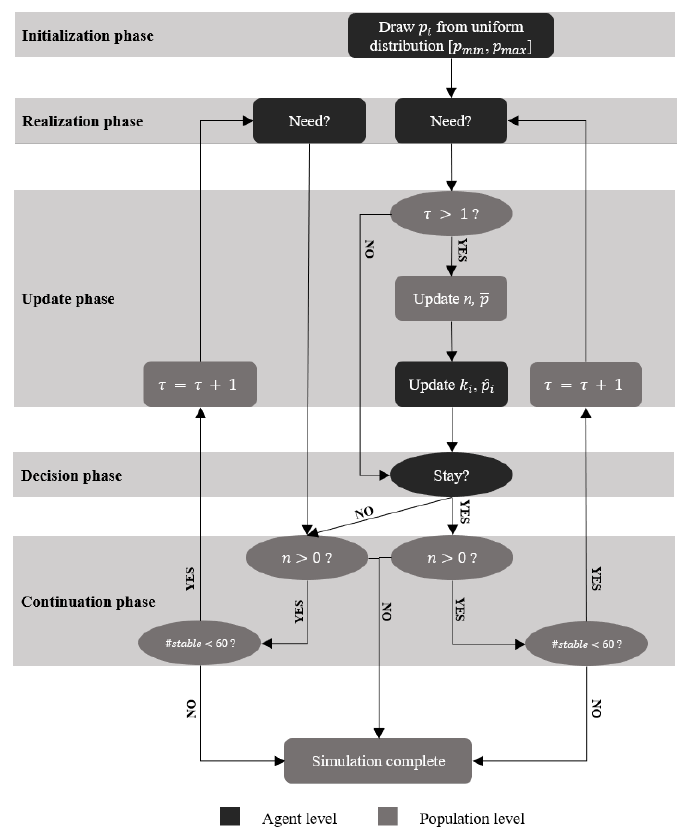
At this point, all agents move back to the realization phase. Only agents that chose to stay move to the update phase, which involves updating population-level parameters \(n\) (the number of members) and \(\overline{p}\) (the average risk) as well as agent-level parameters \(k_i\) (the number of members other than \(i\) that need support) and \(\hat{p}_i\) (the estimated average risk). Subsequently, agents that joined the RSG are brought to another decision phase, while agents that dropped out wait to move to another realization phase. Agents loop over these phases until one of the two stopping conditions is met.
Note that agents only choose to join in the first round; afterwards those who joined choose whether or not to stay. Likewise, since only RSG members move through the update phase, realizations \(k_i\) are informed to members only. Hence, agents cannot wait a few rounds to see how the RSG develops before joining, nor can they, if they chose to leave, revoke this decision later. Without new information about \(k_i\), they do not update \(\hat{p}_i\), and therefore have no incentive to participate in later rounds if they did not before. This is a strict modelling choice, but one justified by the substantive argument that other group members will not reward leaving (a way of defecting) by allowing the defected members to return whenever it suits better. However, it implies that as long as no new members are introduced to the population in later rounds, the RSG can only remain stable or decrease.
At each round, we also calculate whether agents would have participated in the RSG had they known the true risk distribution. In this benchmark Complete Information Model (CIM), agents know the average risk \(\overline{p}\), which means there is no learning involved based on \(\omega\) and \(k_i\). The CIM thus shows the baseline withdrawal pattern expected from the initial distribution and input parameters, recognizing that for some agents the RSG is not interesting to begin with. Deviations between the RSM and the CIM are the result of agents’ responses to fluctuations and thus reflect ‘erroneous’ dropouts.
Data and analysis
Data was stored on the population level for each time point \(\times\) parameter combination for 50 simulations and up until round \(T = 180\). This practical limit was chosen because, if rounds are months, this generates a dataset for what represents a 15-year period.7 This resulted in a dataset with 2,916,000 observations.
Our dependent variable is membership rate: the percentage of agents that remains a member. The main predictor is risk heterogeneity, a categorical comparison of the three conditions that set the boundaries for the populations’ risk distributions: low heterogeneity (LH), intermediate heterogeneity (IH), and high heterogeneity (HH). First, we explored the average stability of the different heterogeneity conditions visually by comparing differences in membership rates between the RSM and CIM. Visualizations of the average risk \(\overline{p}\) are used to assess whether dropout follows adverse selection mechanisms (i.e., low-risk agents drop out, increasing the average risk within the RSGs).
Subsequently, we predicted membership rates for each population using multilevel OLS regressions with simulation runs nested in parameter combinations. Hence, level 1 variance represents stochasticity resulting from the translation of probabilities to events, whereas level 2 variance represents variation in outcomes depending on specific parameter combinations. The analyses are used to give a qualitative description of the simulation results; i.e., to numerically infer when more agents remain part of the RSG. To understand whether population size, risk aversion, solidarity, and learning compensate or strengthen the effect of fluctuations for different risk heterogeneity conditions, we tested for interactions between these variables and risk heterogeneity. Benefit size, previous round dropout (relative to the population size), average estimated risk, and the time period were included as controls. We centered and standardized all continuous variables (i.e., all but the heterogeneity conditions) to compare effect sizes. The analyses were conducted on observations of \(\tau>1\) (because interdependencies in decision-making start from round 2 onwards) and \(\tau\leq60\) (because most groups were stable by that time point).
As a sensitivity check, we ran additional simulations in which we relaxed the core assumption of i.i.d. risks and introduced external correlated shocks. Shocks are inherently present in the simulation model due to the difference between risk and realized support as well as the misconception between true risk and estimated risk. On the aggregate level, however, these effects are not clearly visible. By running multiple simulations over many parameter combinations, we have smoothed this process. Moreover, since shocks are based on the average risk, they are rarely truly out of bound. Hence, we introduce correlated risks—i.e., the simultaneous occurrence of many losses from a single event—to see whether extreme shocks set in motion new withdrawal cascades. We compared three variations where we introduce an external shock of \(p_s=0.5\) (making 50% of the RSG members reliant on support) in one, two, or three consecutive time periods starting from round \(\tau=50\). Since we were primarily interested in what happens in the rounds following the shock(s) a new stopping rule ended all simulations after 80 runs. We ran 30 simulations for each parameter combination, resulting in a new dataset with \(3\times324\times80\times30=2.332.800\) observations.
A second sensitivity check involved an alternative specification of solidarity. Solidarity in the basic model is a fixed trait. To see how sensitive the results are we also studied what happens if solidarity depends on the perceived average risk, decreasing when the negative difference between \(p_i-\hat{p}_i\) increases by multiplying \(\alpha\) with \(\min(1,\frac{p_i}{\hat{p}_i})\). We ran new simulations using the same criteria to obtain a dataset with another 2,916,000 observations (\(324\times180\times50\)) to compare to the original.
Results
Figure 2 plots the decay in membership rates (left panel) and increase in average risk \(\overline{p}\) (right panel) for the three heterogeneity conditions. The general pattern signals adverse selection: as the membership rate decreases, \(\overline{p}\) increases, so the decrease in membership is the result of low-risk agents dropping out. Adverse selection is more severe for the RSM than for the CIM. Under the static CIM, stable participation patterns are still predicted for a substantial share of the population (i.e., 84% for LH, 69% for IH, and 56% for HH under our chosen parameter settings).
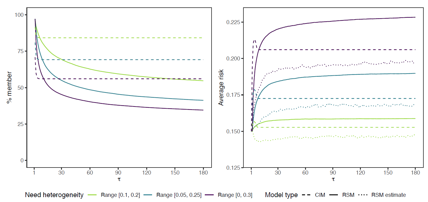
For the RSM, conversely, we can see that despite the agents’ starting assumption that the group’s average risk resembles their own, support requests rapidly increase the average estimated risk \(\hat{p}\) (dotted line in right panel) for all but the LH condition, causing membership rates to drop below the CIM pattern within 10 rounds already (left panel). Hence, while roughly speaking the decay observed for the RSM in the first 10 rounds can be attributed to the fact that the negative \(p_i-\overline{p}\) difference is too big to compensate for by any of the other parameters, the continued drop in membership rate afterwards results from the uncertainty surrounding the true risk \(\overline{p}\), the temporary peaks in support requests \(k\), and the resulting cost fluctuations. Simultaneously, agents do underestimate the average risk. The estimate only starts to catch up to the true average risk when participation decay starts to slow down (after approximately \(\tau=60\)). The slower decrease after \(\tau=60\) suggests that a temporary increase in \(k\) might drive an occasional agent to drop out, but that this no longer invokes cascading effects—a pattern we do observe in earlier rounds.
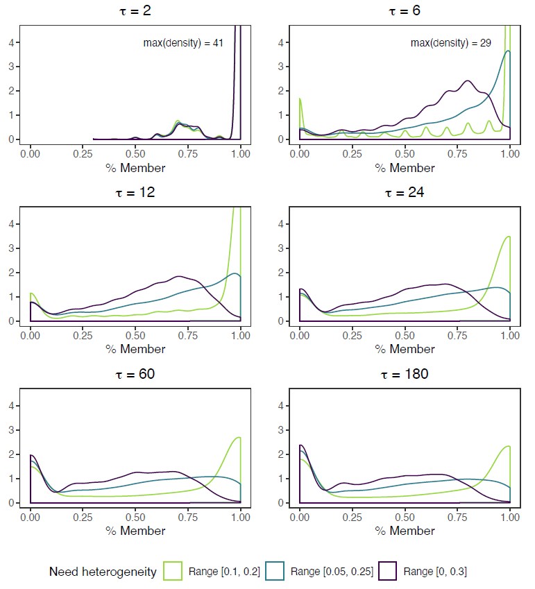
Figure 3 plots the average and distribution of membership rates at time \(\tau = 60\) (see Appendix B for the distribution at different times). It signals the importance of considering not only aggregate membership rates, but also the variation between groups. Lower aggregate averages largely result from failed RSGs. For each heterogeneity condition, the RSM distribution has roughly two peaks (right panel). For LH, the highest peak remains around full membership, but if members withdraw this nearly always ends in complete failure. The other two conditions both moved their main peak from full membership to group failure, but did stabilize more often on alternative, in-between membership rates. Hence, high heterogeneity is less attractive for low-risk agents, but does not automatically lead to cascades. Or rather, while LH groups are more successful in terms of aggregate membership rates, some degree of heterogeneity might be beneficial for the group’s resilience, for dropout of a few members does not necessarily result in complete failure.
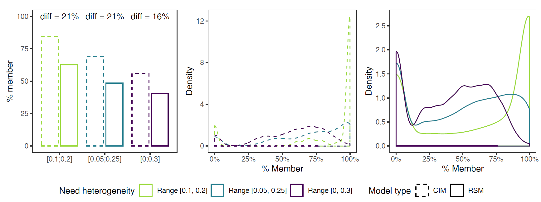
Zooming in on the distribution also shows that failure is much higher than it would have been under complete information. With complete information, total failure would only be expected for 1805 (11%) of 16200 groups, regardless of heterogeneity condition. In the RSM, contrarily, 3625 groups (22%) failed—1297, 1228, and 1100, in the LH, IH, and HH conditions. Hence, about half of the failed groups did so due to cost fluctuations and incomplete information, and complete failure occurs more often in LH groups than in HH groups (a difference of 197 groups or a 18% higher failure rate).
Predicting membership rates from individual motivations
Table 2 outputs the multilevel OLS regressions. Model 1 estimates the main effects and Model 2 includes the interaction terms for \(r\), \(\alpha\), \(\omega\), and \(N\) with risk heterogeneity (taking the LH condition as reference category). Most variance lies on the second level: Model 0 has an intraclass correlation of \(\rho = 0.73\). Hence, most variance is explained from the model parameters. Nonetheless, 27% of the results are driven by stochasticity in \(p_i\) and \(k_i\). This is an important finding: despite favorable starting conditions, RSGs may still risk failure depending on the realization of support requests.
| Model 0 | Model 1 | Model 2 | ||||
| Intercept | 64.902*** | (1.388) | 75.625*** | (0.924) | 75.624*** | (0.909) |
| Range [0.05, 0.25] | -13.887*** | (1.307) | -13.887*** | (1.286) | ||
| Range [0, 0.3] | -23.038*** | (1.307) | -23.035*** | (1.286) | ||
| Risk aversion \(r\) | 17.718*** | (0.534) | 18.630*** | (0.909) | ||
| \(r \times\)Range [0.05, 0.25] | 0.537 | (1.286) | ||||
| \(r \times\) Range [0, 0.3] | -3.271** | (1.286) | ||||
| Solidarity \(\alpha\) | 13.431*** | (0.534) | 14.546*** | (0.909) | ||
| \(\alpha \times\) Range [0.05, 0.25] | -0.380 | (1.286) | ||||
| \(\alpha \times\) Range [0, 0.3] | -2.965** | (1.286) | ||||
| Reinforcement learning \(\omega\) | -3.892*** | (0.534) | -3.874*** | (0.909) | ||
| \(\omega \times\) Range [0.05, 0.25] | -0.226 | (1.286) | ||||
| \(\omega \times\) Range [0, 0.3] | 0.171 | (1.286) | ||||
| Population size \(N\) | 1.567*** | (0.534) | 2.483*** | (0.909) | ||
| \(N \times\) Range [0.05, 0.25] | -0.970 | (1.286) | ||||
| \(N \times\) Range [0, 0.3] | -1.777 | (1.286) | ||||
| Benefit \(b\) | -2.846*** | (0.534) | -2.846*** | (0.525) | ||
| % of members that left | -0.030* | (0.016) | -0.030* | (0.016) | ||
| Estimated average risk \(\hat{p}_i\) | -2.239*** | (0.018) | -2.239*** | (0.018) | ||
| Time point \(\tau\) | -7.463*** | (0.015) | -7.463*** | (0.015) | ||
| Residual variance | 232.24 | 172.68 | 172.68 | |||
| Random intercept | 624.19 | 100.14 | 97.37 | |||
| Intraclass correlation | 0.73 | 0.35 | 0.34 | |||
| Log Likelihood | -3,373,026 | -3,252,181 | -3,252,163 | |||
| Akaike Inf. Crit. | 6,746,059 | 6,504,389 | 6,504,369 | |||
| Bayesian Inf. Crit. | 6,746,094 | 6,504,540 | 6,504,612 | |||
| Notes: \(^{*}p<0.05\); \(^{**}p<0.01\); \(^{***}p<0.001\); Range [0.1, 0.2] used as reference category. | ||||||
The main effects follow the pattern expected from the model input: More risk heterogeneity generates lower membership rates; risk aversion and solidarity increase it; and membership rates decrease the larger the reinforcement learning weight. Population size has a positive influence, indicating that (the effects of) fluctuations are more modest in larger groups. Benefit size has a negative effect, implying that on average costs are higher than the benefits (reflecting low-risk agents that remain part of the RSG anyway). There is a small negative effect of the percentage of members that left at round \(\tau - 1\), but the main driver of the decay observed in is the average estimated risk. The main effects sharply reduce the variance on level 2 (the random intercept drops from 624 to 100), leaving most unexplained variance the result of stochasticity on level 1.
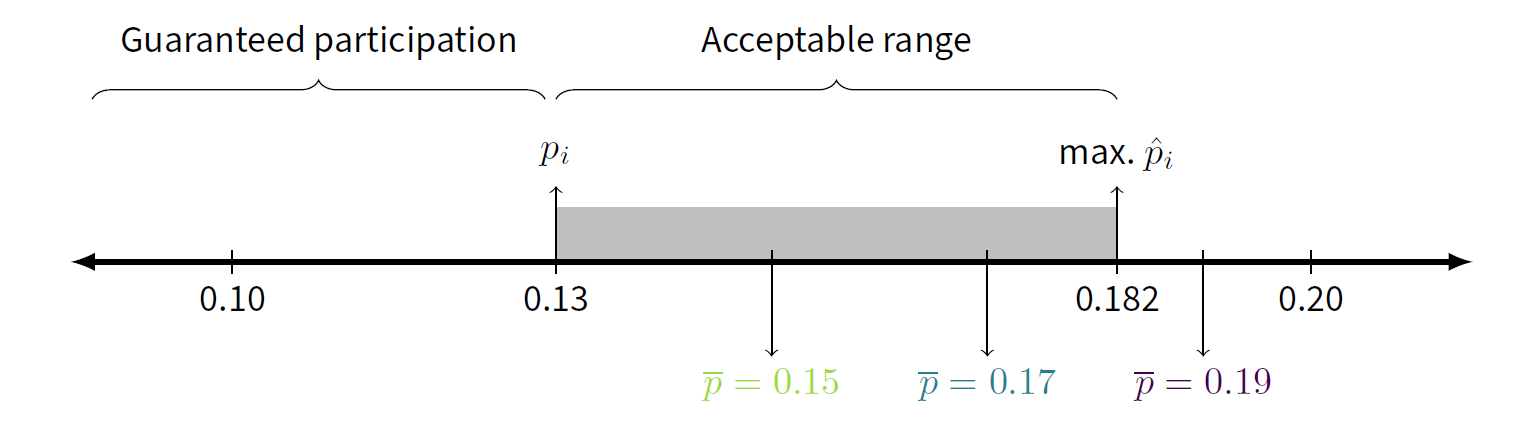
The interactions with the heterogeneity conditions in Model 2 do little to improve the explained variance on level 2 (the random intercept goes from 100 to 97). The only significant interaction effects are related to risk aversion and solidarity. For both, the effects are about 3% points smaller in the HH condition compared to the LH condition, which means that higher levels of risk aversion and solidarity strengthen the negative effect of heterogeneity. In other words, risk aversion and solidarity are more effective in maintaining participation of low-risk agents when risk heterogeneity is small. An example will help to illustrate this finding: let us say an agent has a risk of \(p_i = 0.13\) and solidarity \(\alpha = 0.4\) (assuming no risk aversion). This agent is willing to accept \(\hat{p}_i > p_i\) up until \(\hat{p}_i = 0.13 + 0.4 \times 0.13 = 0.182\) (Figure 4). Since average risk increases more under high heterogeneity, solidarity is less likely to compensate for the increasing costs (they may more easily exceed the acceptable range). For more homogeneous groups, contrarily, minimal solidarity (or risk aversion) is already sufficient to participate even if \(\hat{p}_i > p_i\).
Sensitivity checks
Figure 5 plots the membership decay (top row) and average risk increase (bottom row) for the three correlated shock conditions. The correlated shock has a strong effect in round \(\tau+1\), but does not have a long aftermath in terms of starting new cascades. The learning mechanism, which updates based on the number of support requests, causes the estimated risk to increase steeply, but to decrease equally fast once the correlated shock(s) passed. The effects are detrimental nonetheless, for they greatly reduce membership rates. The longer the shock lasts (and thus the more it impacts average estimated risk), the steeper the total dropout. This holds particularly for the LH condition, where average membership rates after three shocks even end up below the other heterogeneity conditions (Table 3).
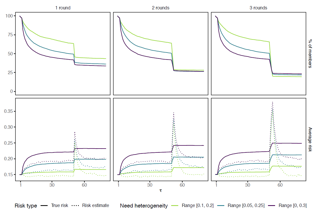
| No shock | 1 at \(\tau = 50\) | 2 at \(\tau = [50,51)\) | 3 at \(\tau = [50,52)\) | |
| Range [0.1, 0.2] | 63% | 44% | 28% | 20% |
| Range [0.05, 0.25] | 49% | 37% | 27% | 22% |
| Range [0, 0.3] | 40% | 35% | 27% | 24% |
That LH groups are affected most can be explained from differences both in risk average and distribution. Since mostly low-risk agents drop out initially, the average risk of the HH groups has increased more (approaching \(\overline{p} = 0.22\) by round \(\tau=50\)). Hence, the difference between the average risk and the temporary shock is smaller in the HH condition, which increases the probability that other factors can compensate for this gap (i.e., the scores on risk aversion and solidarity now also matter for the high-risk agents). Second, in LH groups most agents have approximately the same risk, so once the utility drops below the threshold for one, it also does for most others, because costs and benefits are largely the same for all members.
The second sensitivity check changes the operationalization of solidarity. Recall that we see solidarity not as general altruistic preferences, but as prosocial motives directed towards other members in the risk-sharing group. Solidarity may therefore also increase or decrease depending on group events. For the purpose of addressing limits of risk-sharing arrangements, we considered what happens if in-group solidarity decreases if more people request support. The larger the difference between the estimate of the group’s average risk and one’s own, the smaller the effect of solidarity. Naturally, this has a negative effect on the number of members and on the success of the risk-sharing groups. Figure 6 shows how the membership rates under dynamic solidarity (solid lines) decrease faster than the membership rates under static solidarity (dashed lines). While the drop is substantial, a comparison of membership rates and % of failed groups in Table 4 suggests that the size of the decrease does not depend on the degree of heterogeneity.
The stricter measure of solidarity does not undermine its effect entirely though. Regression analyses (see Table 5 in Appendix C for detailed results) suggest a drop of \(b = 14.546\) (Table 2 to \(b = 10.258\) (Table 5 for the LH condition reference category—i.e., a decrease of about one third. The interaction effect for the HH condition remains more or less the same (\(b = -3.874\) to \(b = 3.385\)). The positive effects of risk aversion \(r\) and population size \(N\) and the negative effect of reinforcement learning \(w\) all slightly increase in strength. Yet in qualitative terms, the main conclusions do not change.
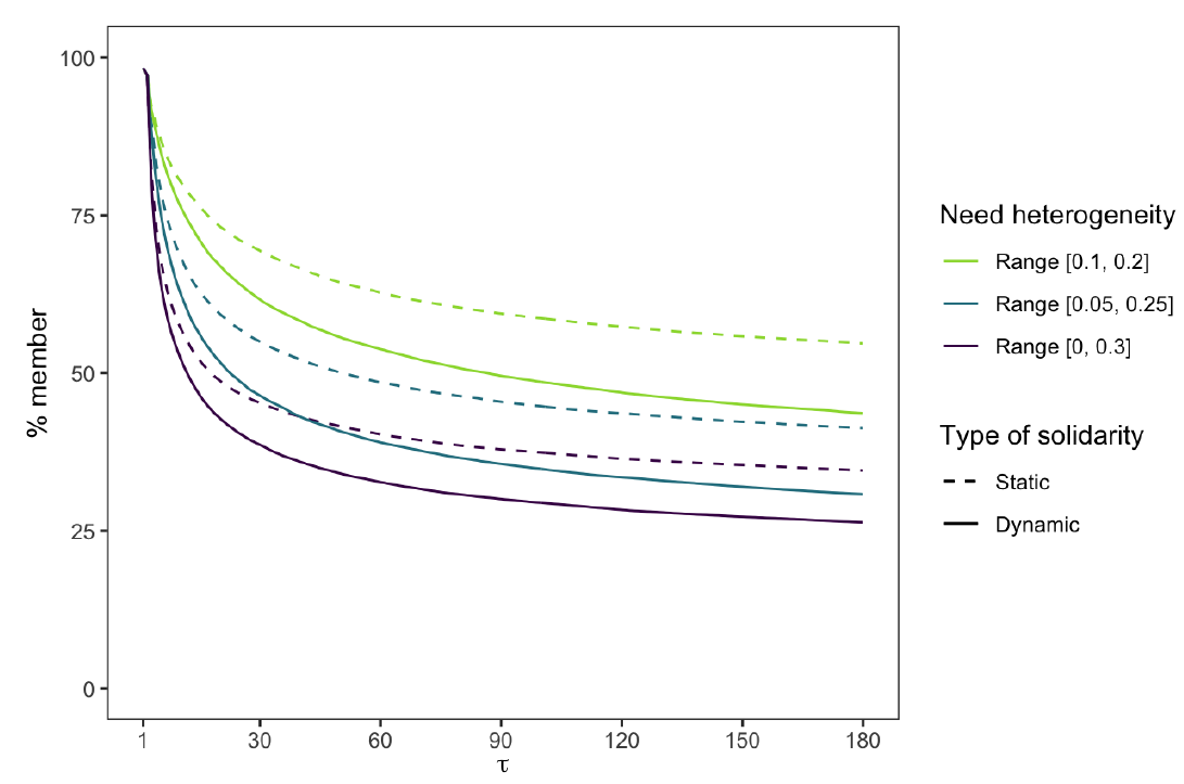
| % member | % failed | |||
| Static | Dynamic | Static | Dynamic | |
| Range [0.1, 0.2] | 63% | 54% | 24% | 30% |
| Range [0.05, 0.25] | 49% | 39% | 23% | 28% |
| Range [0, 0.3] | 40% | 33% | 20% | 25% |
Implications and Hypotheses
From the simulation results we can derive a set of testable hypotheses. The basic implication of risk-sharing under incomplete information corresponds to classic risk-sharing models (Coate & Ravallion 1993; Kimball 1988). Members whose risk is lower than the estimated group’s risk are at risk of dropping out, showing the general tendency of adverse selection. Moreover, we established that if agents update their ideas about the risk of other group members based on support requests (rather than the true risk distribution), participation rates are significantly lower and less stable. As long as the weight attached to these new realizations is small enough, however, decisions remain largely based on the similarity assumption, resulting in the high participation levels predicted also by Skogh & Wu (2005).
Beyond these general results, several dynamics deserve further attention. First, continued membership depends not only on (changes in) support requests, but also on (changes in) the number of members. Hence, if a sudden increase in support requests means that for some members the utility of participating no longer outweighs that of not participating, in the next round other members—who did not have a problem with the increase in the group’s average risk—might also prefer not participating over participating. Not because of new support requests, but because of the decreased number of members. If the costs of supporting group members have to be carried by fewer people, the costs of participation likewise increase. Hence, we derive (H1) that larger numbers of support requests increase the probability of withdrawal cascades, where both other members withdrawing and new support requests cause members to follow each other in deciding to leave the risk-sharing group.
Subsequently, our sensitivity checks indicate that while more heterogeneous groups are less successful overall, they are better equipped to deal with sudden, exceptional increases in support requests. In more homogeneous groups, the high similarity between agents means that if something happens that make participation less attractive for one agent, this is probably true for most of them. Hence, (H2) the more homogeneous the risk-sharing group, the more agents ‘erroneously’ drop out after sudden, exceptional increases in support requests.
Finally, similar to earlier models that study risk heterogeneity (Attanasio et al. 2012; Skogh & Wu 2005; Vogt & Weesie 2004), we included individual factors (risk aversion and solidarity) that can compensate for risk heterogeneity. While these factors could indeed compensate for heterogeneity, they only do so to some extent. The more heterogeneous the risk distribution of a risk-sharing group, the higher risk aversion and/or solidarity have to be to compensate. Thus, (H3) the lower the risk heterogeneity, the stronger the positive effect of (a) risk aversion and (b) solidarity on the likelihood that members stay in the risk-sharing group.
Altogether, these hypotheses make for an interesting theory on the role of risk heterogeneity. More homogeneous groups are, on many accounts, more likely to be established, to succeed, and to maintain high membership rates. Heterogeneous groups, on the other hand, suffer a bigger loss in terms of adverse selection. Yet when they do manage to succeed, they are more resilient to extreme fluctuations in support requests.
Since this difference is the result of incomplete information about the risk distribution, the real threat is not high risk, but a perception of high risk. Each time a sudden increase in support requests results in a spike in estimated risk, agents are at risk of dropping out. This has important implications for the new Peer-to-Peer insurances. To prevent members reacting to sudden and temporary increases in support requests, the organizations must provide clear information about the long-term perspectives of the risk-sharing group. Only then can the impact of exceptionally high support requests be decreased. Another solution is to boost solidarity by stimulating dense and cohesive RSGs. However, these measures may be easier to implement if the group size is smaller, while larger groups were better able to smooth support requests and deal with the occasional drop-out.
Conclusion and Discussion
Engaging in risk-sharing arrangements can be uncertain, fragile, and unstable—but so is the uninsured alternative. So therefore, what are the conditions that underlie participation? What allows stable participation patterns to emerge even under more heterogeneous distributions of risk? A recent revival of mutualism, where so-called Peer-to-Peer insurances set up insurance systems in small risk-sharing groups (RSGs), revived the importance of gaining better theoretical understanding of these questions. After all, other than with regular insurance, RSGs lack the standard institutional arrangements to govern behavior (e.g., mandatory participation or risk differentiation in premium levels) and introduce uncertainty with respect to how often other group members will need support and whether they will continue to participate. That is, two sources of uncertainty that influence the costs of participation.
We constructed a dynamic Risk-Sharing Model (RSM) where members have incomplete information about the risk distribution. Through agent-based simulations we compared how different degrees of risk heterogeneity affects agents’ willingness to be part of the risk-sharing group. Our model showed that membership rates in heterogeneous population are lower on average. One reason is that in more homogeneous groups individual motivations such as solidarity and risk aversion can better compensate for cost fluctuations, for these fluctuations will be less extreme. At the same time, the model predicts that more homogeneous populations—precisely because of their similarity—are less capable of dealing with sudden (large) increases in support requests, making them fragile to internal or external shocks. These results provide potentially important clarifications on the role of heterogeneity in risk-sharing arrangements. While homogeneous RSGs have larger membership rates overall, if members do withdraw this more often results in complete failure. Heterogeneous groups that do survive the start-up phase, on the other hand, are more resilient to sudden external or internal shocks in the long term.
At the same time, it should be noted that with an eye on tractability the model introduced several severe simplifications. We therefore end with a discussion of possible extensions, in increasing order of how much they change the basic RSM, that would further fine-tune theories on the dynamics of participation.
Empirical calibration
The simulations have resulted in several hypotheses that could be tested experimentally, using a risk-sharing setting that follows the set-up of this risk-sharing model. Participants to the experiment would by some probability risk losing their income (and thus earn only the show-up fee for their participation in the experiment). They have the possibility to share this risk with the other (anonymous) participants to the experiment. By assigning them an individual risk but not informing them about the risk of the other group members, it can be estimated whether participation patterns vary across treatments that apply different degrees of risk heterogeneity. The experimental data can be used to test the hypotheses and empirically calibrate the ABM to explore risk-sharing dynamics under realistic values of risk aversion and solidarity.
Stabilizing participation oatterns
The current model set-up is such that member rates can never increase. One model extension to avoid failure would be to introduce a random new batch of agents at several time points. These new agents get the choice whether or not to join the existing RSG, knowing only their own risk and the number of agents that are already participating. While this allows for membership rates to increase, it probably would not solve the heterogeneity problem. Low-risk agents might join initially, but would eventually drop out again, just like the other low-risk agents did before them. High-risk agents do remain, meaning that ultimately we would end up with homogeneous groups of high-risk agents.
The alternative is to implement a more advanced learning parameter. Plain reinforcement learning assumes naive agents (Camerer 2003). More realistic would be to decrease the weight agents attach to support request over time. As they get a better idea of what the true group-level risk is, they should be less affected by sudden peaks in support requests, thus stabilizing participation rates.
Dynamic risk perception
In the current model, people update their estimate of the group’s average risk, but their individual risk remains stable. It is assumed that people know their own risk, or at least have an estimate that is more accurate than their estimate of other people’s risk. Agents participate as long as their estimate of the group risk does not exceed their (estimate of the) individual risk (much). In practice, people’s individual risk perception may vary because despite an objectively low risk probability, they worry about the consequences (Wolff et al. 2019). Such worries may also be driven by changing external consequences, such as increasing risks in other domains (Abdulkareem et al. 2020) or increasing risks of other group members. Such an implementation would, however, ultimately mean that as the estimate of the group’s average risk increases, so does the estimate of an agent’s personal risk. Hence, it would be easier to generate stable participation levels in risk-sharing groups.
Endogenous group formation
Several studies have shown theoretically and empirically that homogeneity preferences play an important role in the formation of RSGs. The simulation results of Hegselmann & Flache (1998), for instance, signal that agents are more likely to engage in risk-sharing when their risk probabilities lie closer together, especially for agents with more extreme risks (either high or low). Attanasio et al. (2012) find experimentally that people are more likely to join a risk-sharing group with close friends and relatives or with people with similar risk attitudes.
In the current setup, agents who drop out are treated as uninterested in risk-sharing arrangements. However, they might have participated had the group’s composition been different. Rather than providing a single risk-sharing setting as an all-or-nothing decision, another possibility would therefore be to let agents choose whether to join one of many RSGs. This does introduce the possibility that agents who now agreed to participate in relatively costly RSGs decide to leave these groups for another, more homogeneous alternative. Introducing endogeneity in group formation increases the number of alternative strategies and could therefore drastically alter the results with respect to how parameters like risk aversion and solidarity affect participation.
Dynamic solidarity
In the current model, solidarity is a personal characteristic that is independent of earlier experiences. In a sensitivity check, we studied what happens if solidarity not only compensates for cost fluctuations, but is also affected by them. It might feel good to help one or two others, but what if one has to support multiple group members without needing help in return? Or what if the same group member repeatedly needs support? Does this only affect participation costs or also one’s solidarity?
While we illustrated the effects of a decay in solidarity over time (Lindenberg 1998), earlier experiences may also increase solidarity. Solidarity could be implemented as following a Markov chain process where current solidarity depends in part on earlier experiences. Solidarity could increase the longer members cooperate, for instance because of increased social embeddedness. Alternatively, when the same agent repeatedly needs support, other agents’ willingness to provide it may have an expiration date. Is the level of solidarity towards the same agent equal after one or ten support requests? An interesting next step would be to model how such dynamics affect solidarity motives over time.
Moral hazard
In the current model, to participate in the RSG is the cooperative strategy, while not participating is considered defection. Another means to defect, however, is not to (no longer) participate in the RSG, but to make fraudulent use of the common fund. A model extension that includes this possibility requires parameters reflecting the probability that such misuse is caught, e.g. through random institutional checks or informal social control. Moreover, the social preferences parameter would have to be extended with a guilt parameter that makes opportunistic strategies less attractive for agents with high solidarity motives (Fehr & Schmidt 1999; Snijders 1996).
Model Documentation
The simulation was programmed in NetLogo (version 6.1.1) and analyzed in R (version 4.0.2). The NetLogo code and model documentation can be retrieved from https://www.comses.net/codebases/3ffb006b-e50f-477d-a1ba-2dce78b9b5e9/releases/1.1.0/ and the model data and R scripts for the visualizations and analyses are stored under hhttps://osf.io/xsyb8/.Notes
The new insurance initiatives cover, e.g., the deductible excess of liability insurance (Friendsurance) or an income replacement for self-employed people in case of sickness (Broodfonds).↩︎
While in reality people do not know their precise individual risk, they at least know more about their own risk than about the risk of other group members. What matters is that they perceive it to be lower or higher than the group’s average, which is captured in this model. The model could be elaborated by adding an error term to the risk such that agents over- or underestimate their own risk, but as long as they use this estimate to compare their own risk to the group’s average that would not change the results.↩︎
Another role of solidarity is that it prevents excessive (fraudulent) insurance claims (i.e., it reduces moral hazard Van Leeuwen 2016). This behavior is not captured in our model.↩︎
The basic set-up assumes there are no operation costs involved. For an institutionalized setting, the profit parameter could be extended to include some administration fee that is paid by all members and reflects a fixed cost.↩︎
While agents may not know their precise risk level, they at least more accurately predict their own risk than that of others.↩︎
In practice, most Peer-to-Peer insurance organizations have similar-sized groups. Friendsurance, for instance, groups members in groups of 10. Broodfonds uses 50 members as a maximum.↩︎
In real-life situations parameters would not remain constant (e.g., risk probability can change over time), we should therefore not use this basic model to interpret cooperation dynamics on very long time scales.↩︎
Appendix
Appendix A: Formal models and derivation of participation conditions
IThe Risk-Sharing Model is built in 3 steps: The baseline model RSM\(_{0}\) compares the utility of participating \(m = 1\) and not participating \(m = 0\) based on rational costs and benefits given individual risk \(p_i\) and the estimated average group risk \(\hat{p}_i\). Model RSM\(_{1}\) includes the individual parameter solidarity \(\alpha\) that offsets the costs of supporting group members. The complete model RSM\(_{2}\) includes the individual parameter risk aversion \(r\) that discounts uncertain outcomes over certain ones.
In RSM\(_{0}\), the expected utilities of participating (\(m = 1\)) and not participating (\(m = 0\)) are:
| \[\begin{aligned} EU = \begin{cases} (1 - p_i)Y + p_i y & \text{if } m = 0\\ (1 - p_i)(Y - c + \hat{\delta}_i) + p_i(y + b - c + \hat{\delta_i}) & \text{if } m = 1. \end{cases}\end{aligned}\] |
If we rewrite \(\hat{\delta}_i = c - \hat{p}_i b - \frac{(\hat{p}_i - p_i)b}{n}\) we obtain for \(m = 1\)
| \[\begin{aligned} EU_{(m = 1)} &= (1 - p_i)(Y - c + c - \hat{p}_i b - \frac{(\hat{p}_i - p_i)b}{n}) + p_i(y + b - c + c - \hat{p}_i b - \frac{(\hat{p}_i - p_i)b}{n}) \\ &= (1 - p_i)(Y - \hat{p}_i(b - \frac{b}{n}) - p_i \frac{b}{n}) + p_i(y + b - \hat{p}_i(b - \frac{b}{n}) - p_i \frac{b}{n}) \\ &=(1 - p_i)Y + p_i(y + b) - \hat{p}_i(b - \frac{b}{n}) - p_i \frac{b}{n}. \\\end{aligned}\] |
For RSM\(_{0}\) we may therefore assume that agents participate if:
| \[\begin{aligned} EU_{(m = 1)} &\geq EU_{(m = 0)} \\ (1 - p_i)Y + p_i(y + b) - \hat{p}_i(b - \frac{b}{n}) - p_i \frac{b}{n} &\geq (1 - p_i)Y + p_i y \\ p_i b - \hat{p}_i(b - \frac{\hat{p}_i}{n}) - p_i \frac{b}{n} &\geq 0 \\ p_i(b - \frac{b}{n}) &\geq \hat{p}_i(b - \frac{b}{n}) \\ p_i &\geq \hat{p}_i.\end{aligned}\] |
In other words, \(p_i(b - \frac{b}{n})\) represent the net benefits of participation and \(\hat{p}_i(b - \frac{b}{n})\) the net costs. In RSM\(_0\), the net benefits outweigh the net costs only if \(p_i >= \hat{p}_i\).
In RSM\(_1\) solidarity is included as parameter \(\alpha\) that defines the extent to which agents are willing to pay the costs of support for their group members. Implemented as \((1 - \alpha)\hat{p}_i(b - \frac{b}{n})\) it compensates for the net costs of participation. This means that for \(m = 1\)
| \[\begin{aligned} EU_{(m = 1)} &=(1 - p_i)Y + p_i(y + b) - (1 - \alpha)\hat{p}_i(b - \frac{b}{n}) - p_i \frac{b}{n}. \\\end{aligned}\] |
For RSM\(_{1}\) we can therefore assume that agents participate if:
| \[\begin{aligned} EU_{(m = 1)} &\geq EU_{(m = 0)} \\ p_i(b - \frac{b}{n}) &\geq (1 - \alpha)\hat{p}_i(b - \frac{b}{n}).\end{aligned}\] |
If we take \(\beta = b- \frac{b}{n}\), we obtain:
| \[\begin{aligned} p_i \beta &\geq (1 - \alpha)\hat{p}_i \beta \\ \alpha \hat{p}_i \beta &\geq \hat{p}_i \beta - p_i \beta \\ \alpha &\geq \frac{\hat{p}_i - p_i}{\hat{p}_i.}\end{aligned}\] |
Hence, in RSM\(_1\) solidarity \(\alpha\) explains that agents may participate even if \(p_i<\hat{p}_i\) as long as \(\alpha\geq\frac{\hat{p}_i-p_i}{\hat{p}_i}\).
Finally, RSM\(_2\) includes risk aversion \(r\). This is operationalized using a concave utility function by adding an exponent \((1 - r)\) to the utility function for both strategies \((m = 1)\) and \((m = 0)\). That is, the utility of each strategy is discounted more for agents who are more risk averse. This yields the final expected utility functions of
| \[\begin{aligned} EU = \begin{cases} (1-p_i)Y^{(1-r)}+p_i y^{(1-r)}, & \text{if } (m=0)\\ (1-p_i) (Y-(1-\alpha)\hat{p}_i \beta)^{(1-r)}+p_i(y+\beta-(1-\alpha)\hat{p}_i\beta)^{(1-r)} & \text{if } (m=1). \end{cases}\end{aligned}\] |
Since the participation conditions of RSM\(_2\) cannot be derived analytically, they are studied through agent-based simulations.
Appendix B: Distributions
Appendix C: Multilevel OLS regressions with dynamic solidarity
| Model 0 | Model 1 | Model 2 | ||||
| Intercept | 59.175*** | (1.308) | 69.658*** | (0.847) | 69654*** | (0.800) |
| Range [0.05, 0.25] | -15.233*** | (1.197) | -15.229*** | (1.131) | ||
| Range [0, 0.3] | -22.994*** | (1.197) | -22.987*** | (1.131) | ||
| Risk aversion \(r\) | 19.133*** | (0.489) | 22.143*** | (0.800) | ||
| \(r \times\)Range [0.05, 0.25] | -2.636** | (1.131) | ||||
| \(r \times\) Range [0, 0.3] | -6.394*** | (1.131) | ||||
| Solidarity \(\alpha\) | 8.524*** | (0.489) | 10.258*** | (0.800) | ||
| \(\alpha \times\) Range [0.05, 0.25] | -1.815 | (1.131) | ||||
| \(\alpha \times\) Range [0, 0.3] | -3.385*** | (1.131) | ||||
| Reinforcement learning \(\omega\) | -4.726*** | (0.489) | -4.962*** | (0.800) | ||
| \(\omega \times\) Range [0.05, 0.25] | -0.083 | (1.131) | ||||
| \(\omega \times\) Range [0, 0.3] | 0.625 | (1.131) | ||||
| Population size \(N\) | 1.770*** | (0.489) | 3.067*** | (0.800) | ||
| \(N \times\) Range [0.05, 0.25] | -1.512 | (1.131) | ||||
| \(N \times\) Range [0, 0.3] | -2.377** | (1.131) | ||||
| Benefit \(b\) | -3.376*** | ;(0.489) | -3.376*** | (0.462) | ||
| % of members that left | -0.313*** | (0.018) | -0.312*** | (0.018) | ||
| Estimated average risk \(\hat{p}_i\) | -2-504*** | (0.020) | -2.504*** | (0.020) | ||
| Time point \(\tau\) | -9.239*** | (0.017) | -9.239*** | (0.017) | ||
| Residual variance | 289.91 | 201.38 | 201.38 | |||
| Random intercept | 554.56 | 77.29 | 68.97 | |||
| Intraclass correlation | 0.66 | 0.28 | 0.26 | |||
| Log Likelihood | -3,351,798 | 3,208,028 | -3,207,99 | |||
| Akaike Inf. Crit. | 6,703,603 | 6,416,081 | 6,416,038 | |||
| Bayesian Inf. Crit. | 6,703,638 | 6,416,232 | 6,416,281 | |||
| Notes: \(^{*}p<0.05\); \(^{**}p<0.01\); \(^{***}p<0.001\); Range [0.1, 0.2] used as reference category. | ||||||
References
ABDIKERIMOVA, S., & Feng, R. (2021). Peer-to-Peer multi-Risk insurance and mutual aid. European Journal of Operational Research, 299(2), 735–749. [doi:10.1016/j.ejor.2021.09.017]
ABDULKAREEM, S. A., Augustijn, E. W., Filatova, T., Musial, K., & Mustafa, Y. T. (2020). Risk perception and behavioral change during epidemics: Comparing models of individual and collective learning. PLoS ONE, 15(1), 1–22. [doi:10.1371/journal.pone.0226483]
ARROW, K. J. (1984). Individual Choice under Certainty and Uncertainty. Cambridge, MA: Harvard University Press.
ATTANASIO, O., Barr, A., Cardenas, J. C., Genicot, G., & Meghir, C. (2012). Risk pooling, risk preferences, and social networks. American Economic Journal: Applied Economics, 4(2), 134–167. [doi:10.1257/app.4.2.134]
BALDASSARRI, D. (2015). Cooperative networks: Altruism, group solidarity, reciprocity, and sanctioning. American Journal of Sociology, 121(2), 355–395. [doi:10.1086/682418]
BALDINI, M., Gallo, G., Reverberi, M., & Trapani, A. (2016). Social transfers and poverty in Europe: Comparing social exclusion and targeting across welfare regimes. DEMB Working Paper Series, Università degli studi di Modena e Reggio Emilia.
BIANCHI, F., Flache, A., & Squazzoni, F. (2020). Solidarity in collaboration networks when everyone competes for the strongest partner: A stochastic actor-based simulation model. Journal of Mathematical Sociology, 44(4), 249–266. [doi:10.1080/0022250x.2019.1704284]
BIANCHI, F., & Squazzoni, F. (2015). Agent-Based models in sociology. Wiley Interdisciplinary Reviews: Computational Statistics, 7(4), 284–306. [doi:10.1002/wics.1356]
BLOCH, F., Genicot, G., & Ray, D. (2008). Informal insurance in social networks. Journal of Economic Theory, 143, 36–58. [doi:10.1016/j.jet.2008.01.008]
BOLTON, G. E., & Ockenfels, A. (2000). A theory of equity, reciprocity, and competition. American Economic Review, 90(1), 166–193. [doi:10.1257/aer.90.1.166]
BREER, V. V., & Novikov, D. A. (2015). Threshold models of mutual insurance. Automation and Remote Control, 76(5), 897–908. [doi:10.1134/s0005117915050148]
BUSH, R. R., & Mosteller, F. (1955). Stochastic Models for Learning. New York, NY: Wiley.
CAMERER, C. F. (1998). Bounded rationality in individual decision making. Experimental Economics, 1, 163–183.
CAMERER, C. F. (2003). Behavioral Game Theory: Experiments in Strategic Interactions. Princeton, NJ: Princeton University Press.
CHAUDHURI, A. (2011). Sustaining cooperation in laboratory public goods experiments: A selective survey of the literature. Experimental Economics, 14(1), 47–83. [doi:10.1007/s10683-010-9257-1]
COATE, S., & Ravallion, M. (1993). Reciprocity without commitment: Characterization and performance of informal insurance arrangements. Journal of Development Economics, 40(1), 1–24. [doi:10.1016/0304-3878(93)90102-s]
DERCON, S., Hill, R. V., Clarke, D., Outes-Leon, I., & Taffesse, A. S. (2014). Offering rainfall insurance to informal insurance groups. Journal of Development Economics, 106, 132–143. [doi:10.1016/j.jdeveco.2013.09.006]
FAFCHAMPS, M. (1992). Solidarity networks in preindustrial societies: Rational peasants with a moral economy. Economic Development and Cultural Change, 41(1), 147–174. [doi:10.1086/452001]
FAFCHAMPS, M., & Lund, S. (2003). Risk-Sharing networks in rural Philippines. Journal of Development Economics, 71, 261–287. [doi:10.1016/s0304-3878(03)00029-4]
FEHR, E., & Gächter, S. (2002). Altruistic punishment in humans. Nature, 415(6868), 137–140. [doi:10.1038/415137a]
FEHR, E., & Schmidt, K. (1999). A theory of fairness, competition and cooperation. Quarterly Journal of Economics, 114(3), 817–868. [doi:10.1162/003355399556151]
FLACHE, A., & Hegselmann, R. (1999). Rationality vs learning in the evolution of solidarity networks: A theoretical comparison. Computational & Mathematical Organization Theory, 5(2), 97–127. [doi:10.1023/a:1009662602975]
GENICOT, G., & Ray, D. (2003). Group formation in risk-Sharing arrangements. Review of Economic Studies, 70(1), 87–113. [doi:10.1111/1467-937x.00238]
GINTIS, H., Bowles, S., Boyd, R., & Fehr, E. (2005). Moral Sentiments and Material Interests: The Foundations of Cooperation in Economic Life. Cambridge, MA: The MIT Press.
GRIMM, V., Berger, U., DeAngelis, D. L., Polhill, J. G., Giske, J., & Railsback, S. F. (2010). The ODD protocol: A review and first update. Ecological Modelling, 221(23), 2760–2768. [doi:10.1016/j.ecolmodel.2010.08.019]
HEGSELMANN, R. (1994). 'Solidarität in einer egoistischen welt: Eine simulation.' In J. Nida-Rümelin (Ed.), Praktische Rationalität: Grundlagenprobleme und Ethische Anwendungen des Rational Choice-Paradigmas (pp. 349–390). Berlin: De Gruyter.
HEGSELMANN, R., & Flache, A. (1998). Understanding complex social dynamics: A plea for cellular automata based modelling. Journal of Artificial Societies and Social Simulation, 1(3), 1: https://www.jasss.org/1/3/1.html.
JIANG, M., & Faure, M. (2020). Risk-sharing in the context of fishery mutual insurance: Learning from China. Marine Policy, 121, 104191. [doi:10.1016/j.marpol.2020.104191]
JORDAN, J. S. (1991). Bayesian learning in repeated normal form games. Games and Economic Behavior, 3, 60–81. [doi:10.1016/0899-8256(91)90005-y]
KIMBALL, M. S. (1988). Farmers’ cooperatives as behavior toward risk. The American Economic Review, 78(1), 224–232.
KIMBALL, M. S. (1993). Standard risk aversion. Econometrica, 61(3), 589–611. [doi:10.2307/2951719]
LIGON, E., Thomas, J. P., & Worrall, T. (2002). Mutual insurance with limited commitment: Theory and evidence from village economies. Review of Economic Studies, 69, 209–244. [doi:10.1111/1467-937x.00204]
LIN, W., Meng, J., & Weng, X. (2019). Formal insurance and informal risk sharing dynamics. Journal of Economic Behavior and Organization, 0(0), 1–27. [doi:10.1016/j.jebo.2019.04.016]
LINDENBERG, S. (1998). 'The problem of solidarity: Theories and models.' In P. Doreian & T. Fararo (Eds.), Solidarity: Its Microfoundations and Macrodependence. A Framing Approach (pp. 61–112). Abingdon: Gordon; Breach Publishers. [doi:10.4337/9781781952863.00016]
LIU, J., & Faure, M. (2018). Risk-sharing agreements to cover environmental damage: Theory and practice. International Environmental Agreements: Politics, Law and Economics, 18(2), 255–273. [doi:10.1007/s10784-018-9386-0]
MACY, M. W., & Flache, A. (2002). Learning dynamics in social dilemmas. Proceedings of the National Academy of Sciences, 99(3), 7229–7236. [doi:10.1073/pnas.092080099]
MACY, M. W., & Willer, R. (2002). From factors to actors: Computational sociology and agent-Based modeling. Annual Review of Sociology, 28, 143–166. [doi:10.1146/annurev.soc.28.110601.141117]
MURGAI, R., Winters, P., Sadoulet, E., & De Janvry, A. (2002). Localized and incomplete mutual insurance. Journal of Development Economics, 67, 245–274. [doi:10.1016/s0304-3878(01)00189-4]
NATALIER, K., & Willis, K. (2008). Taking responsibility or averting risk? a socio-Cultural approach to risk and trust in private health insurance decisions. Health, Risk and Society, 10(4), 399–411. [doi:10.1080/13698570802167413]
OSTROM, E. (1990). Governing the Commons: The Evolution of Institutions for Collective Action. Cambridge: Cambridge University Press.
PLATTEAU, J.-P. (1997). Mutual insurance as an elusive concept in traditional rural communities. Journal of Development Studies, 33(6), 764–796. [doi:10.1080/00220389708422495]
PLATTEAU, J.-P., De Bock, O., & Gelade, W. (2017). The Demand for Microinsurance: A Literature Review. World Development, 94, 139–156. [doi:10.1016/j.worlddev.2017.01.010]
SELLGREN, A. (2001). The evolution of insurance markets under adverse selection. Journal of Evolutionary Economics, 11(5), 501–526. [doi:10.1007/s191-001-8319-z]
SKOGH, G., & Wu, H. (2005). The diversification theorem restated: Risk-Pooling without assignment of probabilities. Journal of Risk and Uncertainty, 31(1), 35–51. [doi:10.1007/s11166-005-2929-0]
SNIJDERS, C. (1996). Trust and commitments. Amsterdam: Thesis Publishers.
TAUSCH, F., Potters, J., & Riedl, A. (2014). An experimental investigation of risk sharing and adverse selection. Journal of Risk and Uncertainty, 48(2), 167–186. [doi:10.1007/s11166-014-9187-y]
TAYLOR-GOOBY, P. (2006). Trust, Risk and Health Care Reform. Health, Risk and Society, 8(2), 97–103. [doi:10.1080/13698570600677092]
TOWNSEND, R. M. (1994). Risk and insurance in village India. Econometrica, 62(3), 539–591. [doi:10.2307/2951659]
VAN LEEUWEN, M. H. D. (2016). Mutual Insurance 1550-2015: From Guild Welfare and Friendly Societies to Contemporary Micro-Insurers. Palgrave Macmillan.
VOGT, S., & Weesie, J. (2004). Social support among heterogeneous partners. Analyse & Kritik, 26, 398–422. [doi:10.1515/auk-2004-0205]
VOGT, S., & Weesie, J. (2006). Social support among heterogeneous partners: An experimental test. Journal of Economic Interaction and Coordination, 1, 215–232. [doi:10.1007/s11403-006-0013-8]
VRIENS, E., Buskens, V., & De Moor, T. (2021). Networks and new mutualism: How embeddedness influences commitment and trust in small mutuals. Socio-Economic Review, 19(3), 1–22. [doi:10.1093/ser/mwz050]
VRIENS, E., & De Moor, T. (2020). Mutuals on the move: Exclusion processes in the welfare state and the rediscovery of mutualism. Social Inclusion, 8(1), 225–237. [doi:10.17645/si.v8i1.2125]
WOLFF, K., Larsen, S., & Øgaard, T. (2019). How to define and measure risk perceptions. Annals of Tourism Research, 79, 102759. [doi:10.1016/j.annals.2019.102759]