Learning Interpretable Logic for Agent-Based Models from Domain Independent Primitives

,
,
,
and
aImprobable Defence, United Kingdom; bCosimmetry, United Kingdom
Journal of Artificial
Societies and Social Simulation 26 (2) 12
<https://www.jasss.org/26/2/12.html>
DOI: 10.18564/jasss.5087
Received: 24-Oct-2022 Accepted: 24-Mar-2023 Published: 31-Mar-2023
Abstract
Genetic programming (GP) is a powerful method applicable to Inverse Generative Social Science (IGSS) for learning non-trivial agent logic in agent-based models (ABMs). While previous attempts at using evolutionary algorithms for learning ABM structures have focused on recombining domain-specific primitives, this paper extends prior work by developing techniques to evolve interpretable agent logic from scratch using a highly flexible domain-specific language (DSL) comprised of domain-independent primitives, such as basic mathematical operators. We demonstrate the flexibility of our method by learning symbolic models in two distinct domains: flocking and opinion dynamics, targeting data generated by reference models. Our results show that the evolved solutions closely resemble the reference models in behavior, generalize exceptionally well, and exhibit robustness to noise. Additionally, we provide an in-depth analysis of the generated code and intermediate behaviors, revealing the training process's progression. We explore techniques for further enhancing the interpretability of the resulting code and include a population-level analysis of the diversity for both models. This research demonstrates the potential of GP in IGSS for learning interpretable agent logic in ABMs across various domains.Introduction
Agent-based models (ABMS) are a powerful tool for building bottom-up models of complex systems by representing many agents individually (Wooldridge 2009). They can recreate emergent phenomena at the macro-level by employing principled and intuitive logic at the micro-level, i.e., individual agents. However, defining these behavioural rules at the agent level is challenging, often requiring a detailed understanding of the underlying micro-level phenomena. Building this understanding can be time-consuming, and intuitions about system dynamics can be misleading. Moreover, there may be situations where insufficient information about the world is available to build an accurate model.
Program syntesis, also referred to as program induction (Manna & Waldinger 1971), is a computational method for generating computer programs from scratch by combining basic symbolic building blocks. For a review of both theory and applications, see David & Kroening (2017) and Gulwani et al. (2017). When genetic algorithms (GAS) are used for program synthesis, this is referred to as Genetic programming (Koza 1992). Genetic programming is a challenging problem for evolutionary search, due to the large, sparse combinatorial search space, as well as the topology of the fitness landscape (Wright 1932), which tends to be rugged instead of smooth, with multiple local maxima separated by low fitness wells or valleys that increase the difficulty of finding and climbing a global maximum.
We propose using program syntesis to partially define the structure of a desired model, requiring only the unknown parts to be synthesised. This enables us to benefit from manually specifying the outer structure of an agent-based model, i.e., code that loops over all agents and executes an individual update function for each one. This encodes the inductive bias that all ABMs share a similar structure, without specifying the contents of the agent update function itself, ensuring that the logic is not constrained by existing priors or domain knowledge.
Our approach focuses on learning agent behavioural rules using genetic programming, allowing the agent-based model to display the macro-level phenomena. By learning agent behavioural rules, we refer to discovering agent behavioural rules through genetic programming.
Our approach can be considered an example of Inverge Generative Social Science (iGSS) (Vu et al. 2019), which is a discovery process for testing multiple hypotheses automatically from data to explain and illuminate observed phenomena. This technique enables us to produce models that are relatively free from existing domain priors and human preconceptions, potentially shedding light on completely new dynamics overlooked because they are unintuitive or non-obvious. The output is an interpretable symbolic model which can be understood and extended by a human modeller, so this could be used for automatically building quick prototype models before a modeller refines them.
We argue that ABMs are a particularly promising application for program synthesis, as complex macro-level behaviors can emerge from simple logic at the individual agent level, which can be encoded with relatively few lines of code in the agent update function. By learning only the relatively concise agent update rules, it becomes feasible to evolve complex emergent behaviors without having to synthesize correspondingly long, complex programs, which remains a challenging problem for current GP techniques.
We applied this technique to learn the agent update function for models in two different domains: flocking and opinion dynamics. Since real data was unavailable, target data was generated by running hand-coded models taken from existing literature. Our approach allowed us to automatically generate ABM logic that closely approximates the target reference datasets.
This work recaps the techniques from Greig & Arranz (2021) and builds on these original experiments to explore the robustness of the training process to noise in the datasets, a deeper analysis of the generated agent logic, and population level analysis of the best solutions. We also explore whether interpretable features can be identified in the learned code and where these features appear over the course of the evolutionary process.
Related Research
The concept of automatically learning the model logic for ABMs has been explored in previous literature, which primarily focuses on learning model structure by modifying existing models. These models are usually already adapted to the specific modeling problem, with a set of domain-specific "primitives" used for recombination. This approach is often called "structural calibration."
For instance, Vu et al. (2019) investigates the evolution of an alcohol consumption model in the US population, aiming to improve its fit to real-world data. The authors employ GP to recombine primitives derived from an initial "tentative" domain model. In this approach, parameter value calibration and structural calibration are conducted in separate optimization steps. The resulting evolved models enable the comparison of different variables’ effects and the evaluation of various hypotheses that could explain the observed data.
Several other studies apply similar structural calibration techniques to various domains, such as opinion dynamics (Husselmann 2015), archaeological simulations (Gunaratne & Garibay 2017), and human crowding models (Junges & Klügl 2011; Zhong et al. 2017). In Zhong et al. (2017), the authors employ a "dual-layer" architecture consisting of a lower-level social force model for collision avoidance and a higher-level navigation model. However, only the navigation model is learned through evolutionary search. In contrast, the flocking experiment in this paper learns the entire model, generating a raw velocity for agents that reflects their collision avoidance tendencies. The techniques presented in this paper could potentially offer more flexibility when applied to crowding problems, eliminating the need for a dual-layer architecture and the social force model assumption.
Additionally, there is a substantial body of research that uses evolutionary algorithms to evolve agent logic for solving cooperation and coordination problems. For example, Koza (1993) evolved a solution to the painted desert problem, while Arranz et al. (2011) evolved a classifier to address a simple cooperative task previously solved using neuroevolution by Quinn (2001). Furthermore, Smith (2008) evolves rules for a classifier determining the social behavior of bird-representing agents. Although these cases produce highly interpretable results, the evolutionary process relies on a fitness function containing built-in domain knowledge.
Unlike the examples mentioned above, which start with existing models or domain-specific primitives, this paper begins with an empty model and utilizes a more flexible DSL. This approach extends structural calibration by eliminating the need for a starting model containing encoded domain knowledge which in turn enables the discovery models with fewer human-imposed assumptions.
Methods
To evolve agent update rules for two different ABMs, namely flocking and opinion dynamics, we employ an evolutionary algorithm. A population of individuals is created, consisting of programs expressed in a domain specific language (DSL). These programs are combinations of the DSL operators and operands. The fitness of each individual in the population is evaluated by executing its program and comparing it to the reference dataset — i.e., the output of a reference model. The best programs are then copied and randomly modified through mutation. This process is repeated until the average fitness (loss) of the population reaches a desired arbitrary threshold.
DSL
Learning useful programs in a general-purpose programming language with complex control flow is still considered to be an open challenge for program syntesis (Shin et al. 2019). This is because these languages are too flexible and result in huge search spaces which are difficult to explore efficiently. As a solution most PS techniques use DSLs, which are constrained programming languages, often subsets of other languages, targeted at a specific use case or domain. Using a DSL significantly reduces the search space of possible programs. It also allows simpler custom mutation rules to be defined which are guaranteed to produce valid, executable programs.
A new DSL is presented in this paper for defining agent logic for ABMs, which is a subset of the programming language Julia (Bezanson et al. 2017). It is comprised of a set of basic mathematical operators which operate on scalar or vector values. It has limited control flow; only IF conditions are allowed, not loops or IF-ELSE statements. This is primarily to reduce the size of the search space. Loops are also avoided because they could increase the execution time of the learned program or result in infinite loops, which would require extra checks to handle. Future work could expand the DSL to incorporate more types of control flow but so far our DSL has shown that is expressive enough to deal with simple ABMs.
Each operator is either a binary or unary function. The set includes simple mathematical operators, however arbitrary Julia functions could be added to this set by the modeller, if desired. The DSL is designed for expressing the agent update function of an ABM, which typically performs some mathematical transformation of their input values, and possibly some conditional operations. Despite these constraints it is still flexible enough to express a wide variety of ABM logic, since more complex mathematical functions can be comprised of simple operations. However, it is not Turing complete because it does not allow loops.
Agent update functions encoded in this DSL are hereafter referred to as behaviours. A behaviour is comprised of a list of instructions, which are interpreted and executed line-by-line as opposed to being compiled, this avoids requiring a time consuming compilation step for evaluating each generated behaviour. Each instruction has an op-code which is the index of an operator from the DSL. It also has input indexes which select the function arguments (these can either be input data about the agent’s environment, numerical parameters or specific memory registers). Instructions store their results in one of a finite number of memory registers, an output index determines which memory register to write to. This is an example of linear genetic programming, and differs from more typical genetic programming approaches which represent the program as a syntax tree and mutate that directly (Koza 1993), rather than a linear list of instructions.
There is a special type of instruction which represents an IF condition, which can branch the program. The op-code specifies a conditional operator such as “less than”, and the output refers to the number of instructions to skip — e.g., the size of the IF block.
Additional configuration is required for the DSL depending on the target modelling problem, including the maximum number of instructions in a behaviour, the number of inputs, numerical parameters, and memory registers.
The set of operators in the DSL can be easily configured. The DSL uses strongly typed instructions, and currently only a single type is supported for a given experiment, either scalar floating point values or 2D vectors. The two experiments in this paper use different types and operator sets, the choice of which is governed by the required output type (2D vector for flocking, scalar for opinion dynamics). This typing adds additional constraints to the DSL, however it is not as restrictive as may be expected, since in the flocking case scalar values can be broadcast to 2D vectors.
The 2D vector operators are as follows: \([-, +, *, \div, square, normalise, norm, clamp, reciprocal, max, min, exp, abs, relu, sin, cos, tan, log, sqrt, <, >, ==, \neq]\). This set of 23 operators was chosen to cover most basic mathematical operations, such as arithmetic, trigonometry and simple linear algebra. A smaller set of 13 scalar operators was used for the opinion dynamics experiment: \([-, +, *, \div, <, >, ==, \neq, square, clamp, reciprocal, abs, identity]\).
Both these sets of operators are much larger, and therefore more flexible, than those used in existing work, for example Gunaratne & Garibay (2017) uses a set of 4 operators and Zhong et al. (2017) uses 6.
Approximate versions of \(==\) and \(\neq\) were used, with a tolerance of 0.001. To avoid causing numerical errors “safe” versions of some functions were used: for \(log\) and \(sqrt\) any negative input values were replaced with a very small positive number close to zero before calling the operation. For trigonometric functions, e.g. \(sin\), any infinite values were replaced with zero.
Genetic algorithm
The genetic algorithm (GA) employed in this study is a re-implementation of the algorithm described in Real et al. (2020) and Real et al. (2019). This algorithm is based on steady-state selection and mutation, but does not include recombination or crossover. In contrast to generational algorithms, steady-state algorithms maintain their population throughout generations, as opposed to replacing it at each generation. For a mathematical analysis of different selection methods, see Goldberg & Deb (1991).
To mitigate early convergence towards local minima and the resulting loss of diversity, the authors also implemented the GA as an island model. Island models, a type of "niching" technique, evolve multiple sub-populations simultaneously while allowing periodic migration between them. The rationale behind this approach is that by evolving several genetic pools in parallel, each can explore different evolutionary trajectories. This increases the overall diversity of the meta-population and slows down convergence (Starkweather et al. 1990). Additionally, island models are easily parallelizable, with each pool running in a separate thread or process, making them highly desirable given the computational costs associated with GP. For more details on the implementation of the evolutionary algorithm, please refer to our previous work in Greig & Arranz (2021).
Loss function
In order to steer the evolutionary process to match the reference data we need an adequate fitness function. Since we are employing data as the source of truth, our fitness function is a loss function between the output of the candidate behaviour and the results from the “true” reference model.
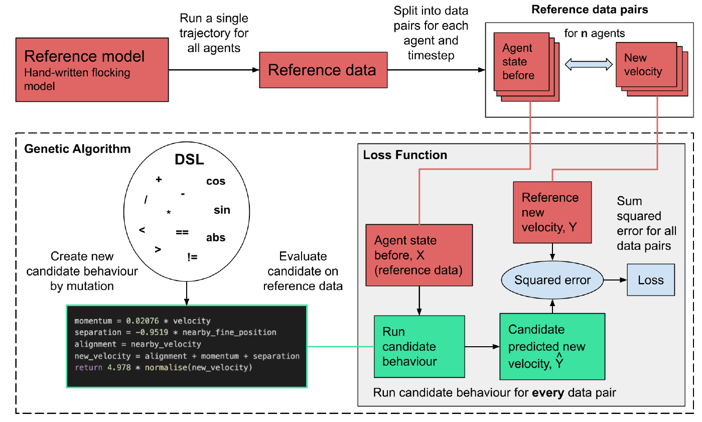
Figure 1 shows how the loss function is calculated, using the flocking model experiment as an example. Firstly the reference dataset is created from the reference flocking model and converted into data pairs of inputs and outputs of the agent update function for every agent at every timestep of the model. The input is the agent’s current state and the state of the surrounding environment (in the flocking model this is the agent’s current velocity, as well as the center of mass and velocities of neighbouring boid agents), and the output is the next value calculated by the true agent update function, in this case the new velocity for the agent.
Since the data pairs can be treated as independent data points, the problem can be approached as a typical supervised learning problem where we want to be able to predict the dependent variable \(Y\) by approximating a function that maps between \(X\) and \(Y\). Here \(Y\) represents the output of the reference agent update function, in this case the new velocity for the agent. If we denote the predicted velocity from the learned behaviour \(\hat{Y}\) and the dataset of all the agent input states \(X\), then the loss function can be expressed as:
| \[loss = \sum_{i=1}^{n} (Y_{i} - \hat{Y}_{i})^2\] | \[(1)\] |
Where \(\hat{Y}\) is calculated using the learned flocking behaviour (steer_behaviour).
| \[\hat{Y}_{i} = steer\_behaviour(X_{i})\] | \[(2)\] |
To evaluate the total loss for a candidate behaviour generated by the genetic algorithm the behaviour is evaluated on every data pair, by passing the “agent state before”, \(X_{i}\), from the reference data as input to the behaviour which gives \(\hat{Y}\). The prediction error for this data pair is then calculated as the difference between \(\hat{Y}_{i}\) and the true output in the reference data, \(Y_{i}\), and summing the square of all these differences across all the data pairs in the reference data to give the total loss for the behaviour.
The agents in the two models presented in this paper — opinion dynamics and flocking — do not have hidden states, this means we can execute the update function independently for each data pair, since the input state from the reference data contains all the required state for each agent. There is no need to run all the timesteps sequentially and pass the output from the previous timestep into the next timestep, as would be the case if the model agents did have hidden state.
Flocking
Flocking models recreate the collective movement of large swarms of animals, such as fish or birds. An influential example is Boids (Reynolds 1987), an agent-based model where individual birds update their velocity based on their nearest neighbours. They use three simple steering behaviours: separation (avoiding collision), alignment (match velocity of neighbours), and cohesion (move towards the average position of neighbours).
This experiment investigates whether the steer function which calculates the velocity of each agent could be synthesised using evolutionary search, starting from scratch with an empty behaviour.
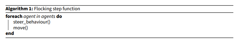
A hand-written implementation of the Boids flocking model was used as a “reference” model to produce target data for synthesising a new behaviour. The pseudocode for the step function which is run for every timestep is shown in Algorithm 1. The aggregate sums of positions and velocities are stored in a spatial grid data structure so agents can efficiently access the position and velocity of neighbours within the same grid cell. Two spatial grids are used at different resolutions; a coarse grid with a cell size of 280 units and a fine grid with a cell size of 12 units. The edge length of the whole grid space is 2000 units.
The reference steer_behaviour() is shown in Listing 1 and contains all of the logic for calculating the new velocity for each agent, this is the function to be replaced by a synthesised version. It takes as input the agent’s own velocity, the relative centre of mass of the neighbours in the same grid cell for both the fine and coarse aggregate grids, the aggregate neighbour velocity relative to the agent’s velocity, and the number of neighbouring agents for both aggregate grids.
function steer(velocity, nearby_velocity, nearby_coarse_position, nearby_fine_position)
	momentum = velocity .* 0.28
	separation = -1 .* nearby_fine_position * 0.03
	alignment = nearby_velocity .* 0.32
	cohesion = nearby_coarse_position .* 0.0015
	target_vel = momentum .+ alignment .+ separation .+ cohesion
	new_velocity = normalise(target_vel) .* 5.0
endThe move() function is a simple physics calculation which adds the newly calculated velocity to the current position. It also handles the logic of wrapping around positions so that the agents move on a toroidal space. This function is not replaced by a synthesised version.
It is clear that the steer behaviour contains the bulk of the logic relevant to the specific flocking domain, i.e. it defines how birds update their velocities in relation to their neighbours. The logic outside this function simply updates the aggregate grids, and updates positions using known velocities. For this reason we say that if the steer function could be synthesised from basic mathematical building blocks, then the flocking model has been learned with minimal a priori domain knowledge.
To produce the target data for the loss function a single trajectory of the reference model was run with 1400 agents for 25 timesteps, which gives 35000 data pairs. Note that the term trajectory here refers to the positions of all agents over time for a single run of the model, not the path of a single agent. The genetic algorithm was run to minimise the loss between synthesised behaviours and the target data, using the set of 2D vector operators listed in the DSL section. The loss calculation only runs the steer() function, using the aggregate positions, velocities and neighbour counts from the target data.
Results overview
The loss decreases significantly throughout the training run, resulting in a loss of 3.558, indicating that the best learned behaviour is able to reproduce the target data very accurately. This experiment took around 8 hours (wall clock time on a n2d-highcpu-32 Google Cloud Instance).
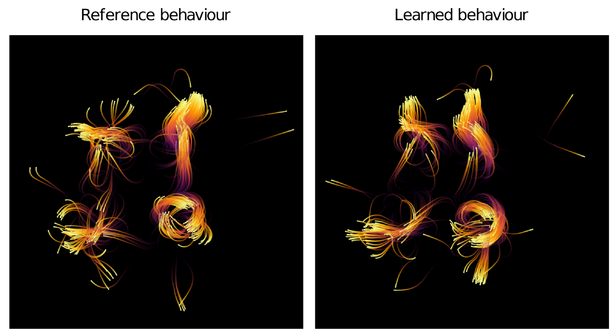
Figure 2 compares the output of the reference model and the best learned behaviour. The plot shows the agent positions after running each model for 80 timesteps, with coloured traces added to show the preceding movement of the agents, the yellow colour indicates more recent positions. Subjectively, these plots show clear similarity in the flocking patterns. Many of the agents are in approximately the same position in both plots, and recognisable movement patterns and clusters of agents can be identified.
We have observed that the model outputs are very similar, however it is also informative to analyse the generated code itself. Listing 2 shows the raw code for the learned behaviour with the lowest loss. This has been converted to valid Julia code, however each line of Julia code corresponds to a specific DSL instruction in the encoded behaviour. This raw generated code is 21 instructions long (not including the code to initialise the temp values to 0.0 which is a feature of the DSL, so is the same in every behaviour and is not learned), this is shorter than the maximum length limit of 32 instructions.
function steer(velocity, _, _, nearby_velocity, nearby_coarse_position, nearby_fine_position)
	params = [-7.019e7, -1.674e9, 111800.0, 8.677e9, -1.648e6, 214.3, 5.427e8, 4.999]
	temp_1 = 0.0
	temp_2 = 0.0
	temp_3 = 0.0
	temp_4 = 0.0
	temp_5 = 0.0
	temp_6 = 0.0
	temp_7 = 0.0
	temp_8 = 0.0
	temp_9 = 0.0
	temp_10 = 0.0
	temp_11 = 0.0
	temp_12 = 0.0
	temp_12 = plus(nearby_velocity, velocity)
	temp_4 = reciprocal(params[7])
	temp_1 = plus(nearby_fine_position, nearby_fine_position)
	temp_7 = safe_cos(params[3])
	temp_8 = safe_sin(params[2])
	temp_2 = plus(nearby_fine_position, velocity)
	temp_4 = minus(params[7], nearby_velocity)
	temp_3 = mult(temp_7, temp_2)
	temp_11 = minus(temp_1, velocity)
	temp_3 = plus(temp_3, temp_12)
	temp_12 = vec_clamp(temp_4)
	temp_1 = plus(nearby_coarse_position, temp_11)
	temp_1 = plus(temp_11, temp_1)
	temp_5 = divide(temp_1, params[6])
	temp_8 = vec_abs(params[5])
	temp_3 = plus(temp_3, temp_5)
	temp_9 = normalise(temp_3)
	temp_12 = mult(temp_9, params[8])
	temp_9 = vec_abs(temp_6)
	temp_5 = reciprocal(params[5])
	return temp_12
endTo aid interpretation of this code, Listing 3 shows a simplified version of the same learned behaviour. This was automatically simplified by converting the encoded behaviour to a computational graph, then performing transformations on this graph such as removing redundant operations that don’t affect the output, and pre-calculating constant values that don’t depend on the input arguments. This simplified representation can then be printed in a readable form as valid Julia code, with multiple instructions combined on the same line, and infix mathematical operators used instead of the DSL function names.
function steer(velocity, _, _, nearby_velocity, nearby_coarse_position, nearby_fine_position)
	c = Vec2(-0.1165,-0.1165) .* ( nearby_fine_position .+ velocity ) .+ ( nearby_velocity .+ velocity )
	h = ( nearby_fine_position .+ nearby_fine_position ) .- velocity
	d = ( h .+ ( nearby_coarse_position .+ h ) ) ./ Vec2(214.3,214.3)
return normalise( c .+ d ) .* Vec2(4.999,4.999)
endFrom the simplified code it is much easier to understand the logic of this behaviour. It calculates a linear transformation of the inputs; \(velocity\), \(nearby\_velocity\), \(nearby\_coarse\_position\), \(nearby\_fine\_position\) by multiplying these by various constants then adding them together. It then normalises the result and multiplies by the constant 4.999, which is equivalent to the reference behaviour (which normalises then multiplies by a constant of 5.0). These 4 inputs correspond to key features of the flocking model: momentum is calculated from the current \(velocity\), separation is calculated from the negative of \(nearby\_fine\_position\) (the center of mass of birds using the fine granularity spatial grid), since the boids want to move away from nearby boids. Cohesion is calculated from \(nearby\_coarse\_position\) (the center of mass of boids using the coarse granularity spatial grid), since the boids want to move towards large groups of nearby boids, and alignment is calculated from \(nearby\_velocity\).
Note that in Listings 2 and 3 there are two function arguments represented by an underscore, which means that these inputs were available but this learned behaviour does not use them. These arguments are \(nearby\_coarse\_count\) and \(nearby\_fine\_count\), which are the number of neighbouring boids in the coarse and fine spatial grids respectively.
Evolutionary trajectories
During the flocking training runs the loss tended to decrease not smoothly but in large transitions or “jumps”, which were found to correspond to “innovations” where the generated model had discovered new features. This is reminiscent of “punctuated equilibria” in evolutionary theory (Eldredge & Gould 1971). These jumps due to innovations are explored in more detail below for this flocking training run.
As discussed earlier the boids flocking reference model has three key dynamics: alignment, separation and cohesion. It also has a momentum term, which is calculated from each boid’s previous velocity. After the new velocity vector is calculated from these four terms in the reference model it is normalised so that all velocities have the same magnitude. The training process learns a symbolic model that has all of these features: momentum, alignment, separation, cohesion and normalisation, and is therefore able to recreate the reference dataset very accurately. As the training run progresses we can inspect when these different features appear and in what order by analysing the intermediate generated code and plotting the output from running this code.
Figure 3 shows the progression of a training run for the flocking model, along with some intermediate output results visualised at key points in the training run. There are two notable transition points which correspond to large drops in the loss, these are analysed below.
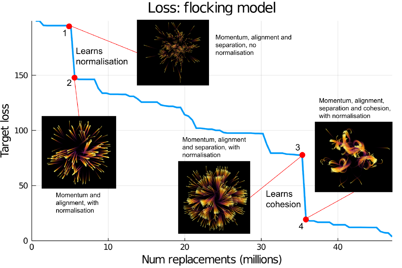
Transition \(\mathbf{1 \rightarrow 2}\): Learning normalisation
The transition between points 1 to 2 marked on Figure 3, corresponds to the generated model learning to normalise the output velocity vector so that all birds have a constant speed. Here the loss drops from 193.6 to 146.9. By point 1 the model has already learned the concepts of momentum, alignment and separation, which it learns very early in the training run, however before this point it is not normalising the output vector. This means that the boids all have different magnitudes of velocities, this is apparent in the “trails” visualisation of the model output shown at point 1; each trail shows an individual boid’s position over time, at point 1 the trails all have different lengths, meaning they are moving at different speeds because there is no normalisation to make the velocities have a constant magnitude. However at point 2, after it has learned normalisation, the trails all have approximately the same length, showing that the magnitudes of the velocities are equal.
This transition can also be seen in the generated code at points 1 and 2. Listing 4 shows the generated flocking code at point 1 (NB: all generated code at the transition points has been automatically simplified in the same manner as Listing 3). At point 1 the code contains momentum, alignment and separation (due to using \(velocity\), \(nearby\_velocity\) and \(nearby\_fine\_position\)), however before the new velocity is returned it performs a minimum operation with a constant vector, instead of normalising it. However at point 2, code shown in Listing 5 it uses the \(normalise\) function in the DSL to normalise the returned new velocity vector. This also contains an unnecessary IF condition comparing the nearby_coarse_count to a constant, however for most input values this seems to result in normalising the velocity rather than returning the raw velocity vector.
function steer(velocity, _, _, nearby_velocity, _, nearby_fine_position)
	a = safe_tan( nearby_fine_position ./ Vec2(13.82,13.82) )
	return vec_min( Vec2(4.81,4.81), velocity .- a .+ nearby_velocity )
end
function steer(velocity, nearby_coarse_count, _, nearby_velocity, _, _)
	d = nearby_velocity .+ velocity
	i = if not_equal_to( Vec2(-661.9,-661.9), relu( velocity ) )
		normalise( d ) .* Vec2(4.866,4.866)
	else
		d
	end
	b = if less_than( Vec2(9.748,9.748), nearby_coarse_count )
		i
	else
		d
	end
	return b
endTransition \(\mathbf{3 \rightarrow 4}\): Learning cohesion
The transition between points 3 and 4 marked on Figure 3, corresponds to the generated model learning cohesion, meaning that boids move towards the center of mass of the nearest group of other boids. This has a marked effect on the output; at point 3 and before, the boids’ velocity has a mostly constant direction, which appears on the trails plot as straight lines radiating out from the origin. However once cohesion has been learned at point 4 the trails are curved towards nearby groups of boids, characteristic of flocking motion.
The incorporation of cohesion can be seen in the code in Listing 7, where the cohesion term is calculated from the \(nearby\_coarse\_position\) input, which represents the center of mass of nearby boids using the coarse (larger grid cells) spatial grid. This term is absent in the generated code at point 3, which can be seen in Listing 6.
function steer(velocity, _, _, nearby_velocity, _, nearby_fine_position)
	e = Vec2(-0.09124,-0.09124) .* ( nearby_fine_position .+ velocity ) .+ ( nearby_velocity .+ velocity )
	g = velocity ./ Vec2(36.55,36.55)
	return normalise( e .- g ) .* Vec2(4.978,4.978)
end
function steer(velocity, _, _, nearby_velocity, nearby_coarse_position, nearby_fine_position)
	l = Vec2(-0.1052,-0.1052) .* ( nearby_fine_position .+ velocity ) .+ ( nearby_velocity .+ velocity )
	h = if greater_than( Vec2(84860.0,84860.0), vec_clamp( safe_tan( nearby_fine_position ) ) )
		l .+ nearby_coarse_position ./ Vec2(222.1,222.1)
	else
		l
	end
	return normalise( h ) .* Vec2(4.981,4.981)
endLearning and forgetting separation
It is notable that at point 2 even though the model has learned normalisation, it seems to have “forgotten” separation which is present at point 1, although even without separation this results in a much lower loss than point 1. Somewhere between points 2 and 3 the model re-learns separation, now combined with momentum, alignment and normalisation. This difference in separation is apparent in the trails plot, at point 2 the trails plot shows thicker straight lines, which represents clusters of boids clumped closely together, however the plot at point 3 shows that the boids are spread out from each other due to the separation behaviour, resulting in thinner lines of individual boids moving away from each other.
This re-learning of separation happens during a period of gradual decrease in loss, so it does not appear as a large “transition” and it is difficult to pinpoint exactly where this occurs.
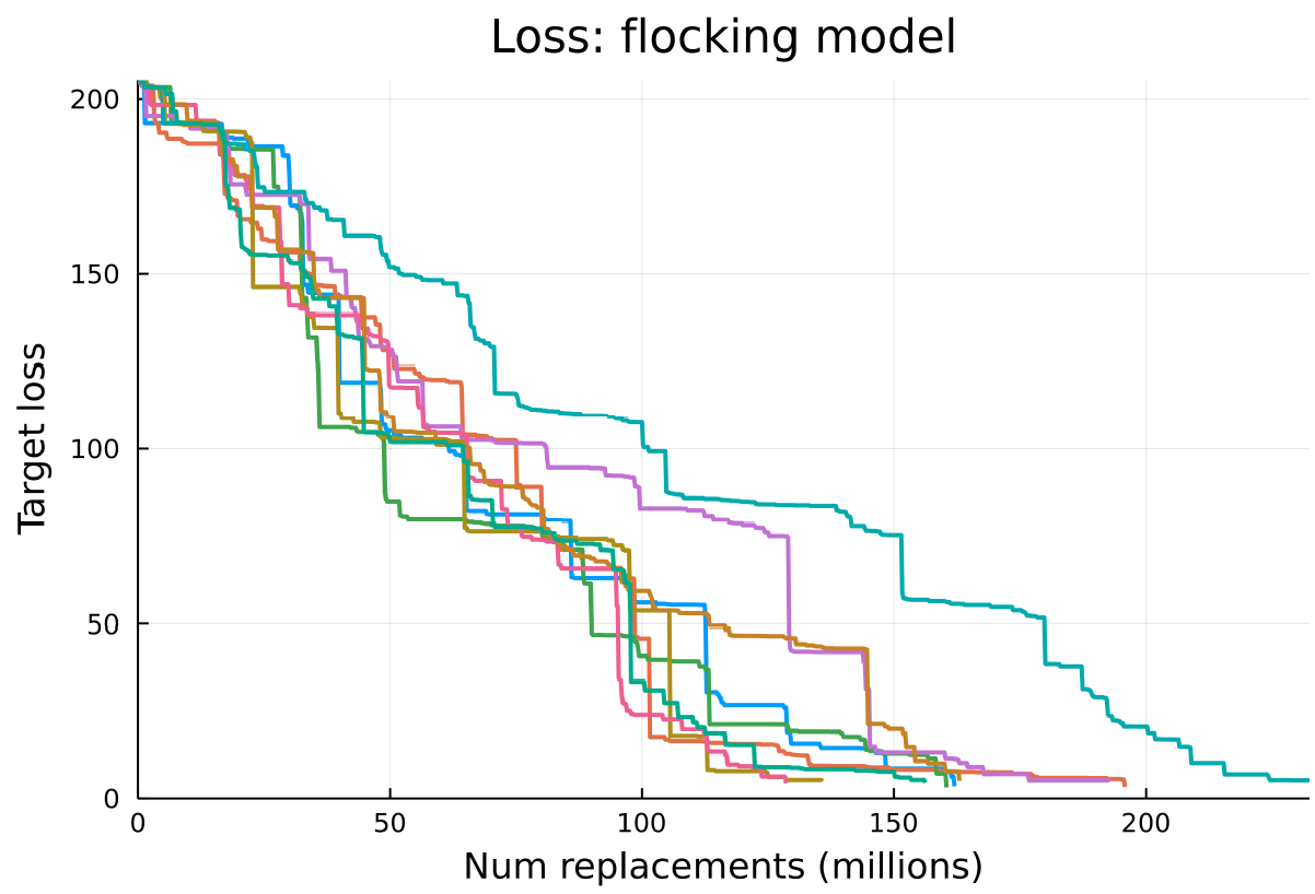
Analysis of multiple training runs
A further 9 repetitions of the flocking experiment were conducted with the same configuration, except for the number of pools, which was increased from 64 to 200 in order to take further advantage of parallelisation across multiple processor cores. The aim was to assess whether the same transitions occurred and if features were learned in the same order. Figure 4 shows the loss for all 9 repetitions. All the training runs successfully achieve a low loss, and take approximately similar amounts of time to do so, however they have varying sizes of “jumps” in loss, and the jumps occur at different times. Additionally not all jumps seem to correspond to learning the same features across runs. From analysing the generated code and output of the learned behaviours it was determined that that not all of the training runs learn the flocking model features in the same order.
However there are some commonalities between the runs. Momentum and alignment were always learned first, very early in the training run. It also seems fairly common that some features are forgotten and then re-learned, like separation in the original training run. There are examples of both separation and cohesion being forgotten then re-learned.
The most common order of learning features seems to be: normalisation, separation, then cohesion, this order is present in 5 out of 9 runs, as well as the original run. In some runs cohesion is learned before separation. Cohesion normally appears fairly late in the run. Out of these three features normalisation is always first, perhaps this is an easier feature to learn, or perhaps there is some inherent reason for this ordering, for example perhaps without normalisation it makes it harder to learn the other features.
Generalisation
The solutions evolved by the genetic algorithm are capable of replicating the macro behaviours of both models with high accuracy. A recurring issue with traditional AI/ML techniques is over-fitting of the solutions to the training data, meaning that the models are not able to perform adequately in new situations — i.e., with new data. Evolutionary computation and genetic algorithms are no exception as they are also prone to over-fitting — e.g., Gonçalves & Silva (2011), Gonçalves et al. (2012), Langdon (2011). This is particularly problematic in cases where the training data-set is relatively small, noisy or incomplete.
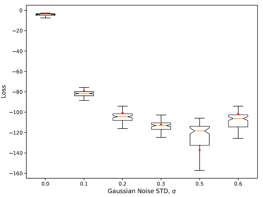
To find out how well the best solution perform with out-of-sample data — i.e., trajectories of the model which have not previously seen during training/evolution — we ran new series of experiments in which we compare the output of the reference implementation and the output of the best evolved solution for 1000 different trajectories of the models. We plot the distribution of those loss values for each of these trajectories. The results of these runs are shown in Figure 5. The first box-plot in the figure clearly shows the remarkable robustness — i.e., low variance and median — of the best evolved solution when evaluated against to 1000 random seeds of the model compared to the reference run (red dot).
We also investigate the effect of increasing levels of Gaussian noise on the performance of the evolved solutions (Figure 5). It is known that in some cases input noise can increase the robustness of the evolved solutions — e.g., Arranz et al. (2011) for an example where a small amount of Gaussian noise in the input data leads to a more robust solution. In our particular case, there is a very small margin for improvement as we speculate that the best evolved candidates are logical clones of the reference model — i.e., close to perfect solutions. Any improvement over the solutions trained with noiseless data are likely to relate on the accuracy of the fixed numerical parameters rather than on the program logic itself. In the case of the flocking model, the results in Figure 5 appear to confirm that assumption, as such, we do not observe any decrease in the loss when Gaussian noise is added. It is important to clarify that the evaluation of the solutions evolved with noisy/incomplete data is performed against a completely noiseless reference data set.
Population level analysis
Up to this point our focus has been on understanding the best candidate solution and figuring out how it works and how it evolves. Still, there are other solutions in the final population that also reach high fitness scores. This can be suggestive of the existence of qualitatively different and potentially non-intuitive solutions or solutions that are qualitatively different to our reference model.
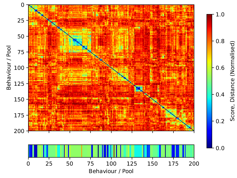
We are interested in determining the diversity of the solutions that the algorithm evolves, i.e., the solution landscape. With this in mind, we visualise the landscape in terms of solution similarity/distance in the program space. We compute the Hamming distance of the best candidate behaviours in each one of the pools in the last generation of a training run. We construct a distance matrix and re-order it to cluster similar behaviours. Our goal is to understand the solution landscape in terms of fitness and program closeness. The overall population appears considerably diverse in terms of Hamming distance – reddish areas of the similarity matrix in Figure 6. We observe several sub-populations — in blueish — around the diagonal with several fitness values. Interestingly those sub-populations do not always map to high performing behaviours. For instance, the fittest behaviour in the population appears to be rather isolated (index 101 in Figure 6 and Listing 8). However, the second best behaviour (index 67, Listing 8) does indeed belong to a big sub-population of similar behaviours around indices from 50 to 75 in Figure 6. When compared, it is clear that both programs differ significantly.
It is important to clarify that different solutions in program space can potentially map to the same solution in logical space. We understand logical space as the core algorithm or strategy of a behaviour which is independent on its implementation. This would be equivalent to different language implementations — e.g., C, Python, Julia — of the same algorithm — e.g., the Quicksort algorithm. In this example, the logical space would be Quicksort algorithm and the program space would be any implementation of the algorithm. We leave this kind of analysis for future work as it requires a new set of non-trivial tools that can simplify and translate the candidate programs to logical graphs and calculate their similarity in logical space instead of program space. Preliminary results in that direction
We also notice a lack of continuity between very similar behaviours and their corresponding fitness scores. This is suggestive of a rough fitness-similarity mapping landscape, i.e., small changes in the programs might result in wildly different outcomes in simulation space. This is expected as the mutation of a single operator — and therefore a single unit of distance — can entirely change the outcome of the behaviour.
// Candidate Behaviour with index 103 (1st) with loss -3.5489087
function evaluate(velocity, nearby_coarse_count, nearby_fine_count, nearby_velocity,
	nearby_coarse_position, nearby_fine_position)
	safe_sin_7 = safe_sin( safe_sin( Vec2(-0.11408108998369672,-0.11408108998369672) )
	.* nearby_fine_position )
	divide_2 = nearby_velocity ./ Vec2(7.553817851654282,7.553817851654282)
	plus_14 = ( divide_2 .+ nearby_velocity ) .+ vec_min( safe_sqrt( safe_sin_7 ), safe_sin_7 .+ divide_2
	./ Vec2(12.219124714836855,12.219124714836855) )
	divide_16 = ( velocity .+ plus_14 ) ./ Vec2(1.312095042167458,1.312095042167458)
	if not_equal_to( Vec2(-0.11408108998369672,-0.11408108998369672),
		vec_exp( Vec2(7.553817851654282,7.553817851654282) ) )
		conditional_39 = safe_log( Vec2(147.16264617902266,147.16264617902266) )
		conditional_38 = reciprocal( nearby_fine_count )
		conditional_37 = vec_min( nearby_fine_position, nearby_coarse_count )
		conditional_40 = normalise( divide_16 .+ nearby_coarse_position
		.* Vec2(0.004052771092348564,0.004052771092348564) )
	else
		conditional_39 = Vec2(0.0,0.0) .* divide_2
	conditional_38 = normalise( Vec2(0.0,0.0) )
	conditional_37 = plus_14
	conditional_40 = divide_16
	end
	return conditional_39 .* conditional_40
end

// Candidate Behaviour with index 67 (2nd best) with loss -6.1179295
function evaluate(velocity, nearby_coarse_count, nearby_fine_count, nearby_velocity,
	nearby_coarse_position, nearby_fine_position)
	vec_norm_11 = vec_norm( Vec2(0.004052771092348564,0.004052771092348564) )
	vec_abs_20 = vec_abs( reciprocal( Vec2(147.16264617902266,147.16264617902266) ) )
	vec_abs_19 = vec_abs( Vec2(4.444026824818702,4.444026824818702) )
	safe_log_14 = safe_log( Vec2(147.16264617902266,147.16264617902266) )
	safe_sqrt_17 = safe_sqrt( safe_log_14 )
	mult_5 = safe_sin( Vec2(-0.11408108998369672,-0.11408108998369672) ) .* nearby_fine_position
	divide_2 = nearby_velocity ./ safe_sqrt( Vec2(48.87649885934742,48.87649885934742) )
	plus_13 = ( velocity .+ ( ( divide_2 .+ nearby_velocity )
	.+ ( mult_5 .+ Vec2(0.0,0.0) ) ) )
	./ Vec2(1.312095042167458,1.312095042167458) .+ nearby_coarse_position
	.* Vec2(0.004052771092348564,0.004052771092348564)
	mult_12 = nearby_fine_position .* velocity
	minus_16 = Vec2(4.444026824818702,4.444026824818702) .- nearby_coarse_count
	return safe_log_14 .* normalise( plus_13 )
endOpinion Dynamics
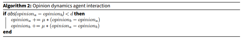
To demonstrate the generality of the PS technique introduced in this paper, it is important to show that it can learn models in multiple domains. To show this, an opinion dynamics model was chosen as an alternative. The model is a simple threshold model, as described in Deffuant et al. (2000). This model simulates how opinions on a topic spread amongst a population of agents. The basic model with complete mixing was used, meaning that agents can interact with any other agent, and these interactions are chosen randomly with a uniform distribution. Each agent has an opinion represented by a real number between 0 and 1. For an interaction 2 agents are selected, if the difference between their opinion values is below a threshold, \(d\), then they each move their opinions towards the other, according to a convergence parameter \(\mu \in \mathbb{R} \cap [0, 1]\). The logic for this interaction is shown in Algorithm 2. The threshold logic is motivated by the idea of homophily, meaning that two agents only move their opinions if they are already close to each other.
The interaction function in Algorithm 2 was chosen as the target to be learned. As with the flocking model, this function contains the core domain logic of the model, the surrounding code simply selects which agents interact with each other. One difference from the flocking model is that this target behaviour requires control flow in the form of conditional logic, so that the opinions only get updated if they are already within the threshold. Learning conditional logic presents an additional challenge for the PS search process. Even though the code in Algorithm 2 is only 4 lines long, this actually corresponds to 11 instructions when encoded in the DSL, because each DSL instruction can only execute 1 operation at a time and write the result to a memory register, so all intermediate calculations must be performed with separate instructions. This is highlighted to show that this still presents a potentially challenging task for PS. This experiment used the set of scalar operators listed in the DSL section.
The reference data for the loss calculation is the before and after state of each agent’s opinions for every interaction. To produce this, the reference model was run with 1000 agents for 25 timesteps, with 1000 interactions per timestep, which gives 25000 data pairs. The threshold, \(d\), was set to 0.2, and the convergence parameter, \(\mu\), was set to 0.5. As with the flocking experiment, only one trajectory — i.e., a single run — from the reference model was used for training.
Results overview
As with the flocking experiment, the opinion dynamics training run is also successfully able to replicate the reference behaviour, achieving a loss of 0.051.
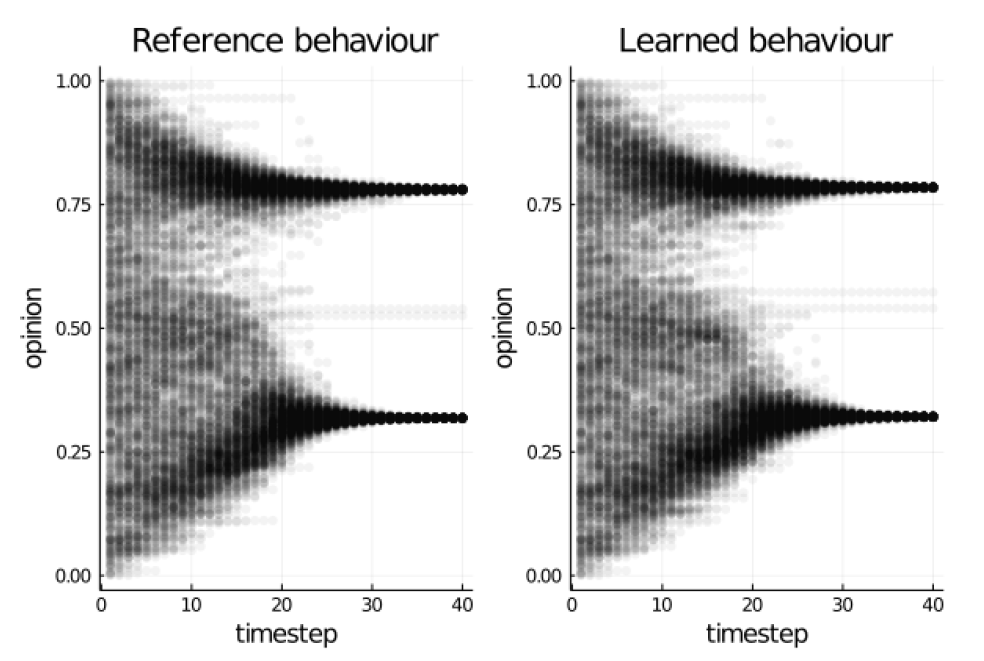
The outputs from running the reference and learned behaviours are compared in Figure 7. These plots show how the opinions of each agent change over the course of a model run. The learned behaviour is able to produce output that is almost identical to the reference model, as would be expected given the loss achieved during training. In both sets of results there are two main clusters of opinions, which is the main characteristic of the model output discussed in (Deffuant et al. 2000).
Listing 9 shows the raw generated code and for the best learned behaviour. Listing 10 shows a version which has been automatically simplified in the same manner as Listing 3. The raw code contains some empty IF conditions and redundant instructions, it is also harder to interpret. The raw code is 20 instructions long, which hits the limit of 20 instructions for this experiment. The simplified code is slightly shorter, and could be shortened even further by combining more operations onto the same line.
function update_opinion(opinion_a, opinion_b)
	params = [-44.4, 0.08822]
	temp_1 = 0.0
	temp_2 = 0.0
	temp_3 = 0.0
	temp_4 = 0.0
	temp_3 = plus(temp_3, temp_1)
	temp_1 = minus(opinion_a, opinion_b)
	temp_3 = minus(params[1], opinion_a)
	temp_4 = divide(temp_1, temp_3)
	temp_1 = mult(temp_1, temp_1)
	temp_2 = square(temp_1)
	temp_1 = minus(params[2], temp_1)
	temp_1 = minus(temp_1, temp_2)
	temp_1 = plus(params[2], temp_1)
	temp_1 = mult(temp_1, temp_4)
	temp_4 = divide(temp_4, params[2])
	temp_3 = plus(opinion_a, temp_4)
	temp_1 = scalar_abs(temp_1)
	temp_3 = plus(temp_3, temp_4)
	if not_equal_to(temp_2, temp_1)
		if not_equal_to(params[1], opinion_b)
			temp_4 = minus(temp_2, temp_2)
		end
		temp_3 = no_op(opinion_a)
	end
	if greater_than(temp_2, temp_2)
	end
	temp_4 = minus(opinion_b, temp_4)
	return temp_3, temp_4
end
function update_opinion(opinion_a, opinion_b)
	j = opinion_a - opinion_b
	l = j * j
	s = square( l )
	f = j / ( -44.3959 - opinion_a )
	r = f / 0.0882
	i = if ( !isapprox(-44.3959, opinion_b, atol=0.001) )
		s - s
	else
		r
	end
	c = ( 0.0882 - l ) - s
	if ( !isapprox(s, scalar_abs( ( 0.0882 + c ) * f ), atol=0.001) )
		p = i
		d = opinion_a
	else
		p = r
		d = opinion_a + r + r
	end
	return d, opinion_b - p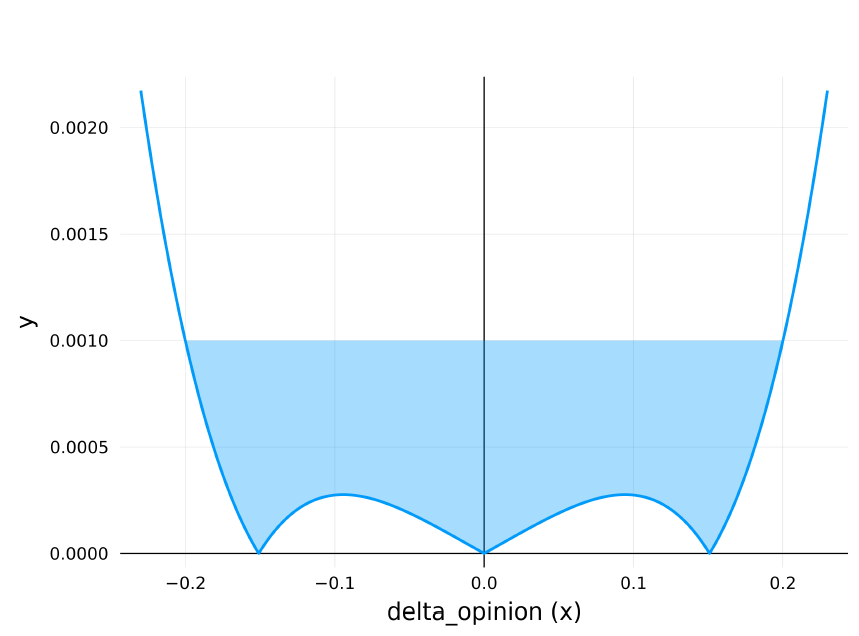
endNotably this learned behaviour appears to have exactly recreated the threshold logic of the reference behaviour, but in an alternative way; by learning a polynomial function of the difference between the two input opinions, \(delta\_opinion\). Different variables in the code correspond to different powers of \(delta\_opinion\); \(j = delta\_opinion\), \(l = delta\_opinion^2\) and \(s = delta\_opinion^4\). The \(isapprox(a, b)\) function is equivalent to \(abs(a - b) < 0.001\), since there is an absolute tolerance of \(0.001\). This gives us an expression for the input of the second IF condition of:
| \[abs(s - abs( ( 0.0882 + c ) * f)) < 0.001\] | \[(3)\] |
This can be rearranged in terms of \(delta\_opinion\), if we let \(x = delta\_opinion\), to give
| \[abs(x^4 - abs(\frac{0.1764x - x^3 - x^5}{-44.3959 - opinion\_a})) < 0.001\] | \[(4)\] |
If we approximate \(-44.3959 - opinion\_a \approx -44.3959\), since \(opinion\_a\) is typically between 0.0 and 1.0, and therefore much smaller than \(-44.3959\), then can be reduced to an expression of only x terms:
| \[abs(x^4 - abs(0.02252x^5 + 0.02252x^3 - 0.00397x)) < 0.001\] | \[(5)\] |
A plot of this polynomial inequality is shown in Figure 8, the line \(x=0.001\) is plotted, anywhere the polynomial function is below this line (filled in blue on the plot) the \(isapprox\) function in the second IF condition evaluates to true, determining which code branch is taken. It can be seen that the cutoff intercept points for this are at \(x=\pm0.2\), this corresponds exactly to the threshold value \(d=0.2\) used in the reference model. This second IF condition is therefore equivalent to the reference model logic which only updates the output opinions if \(abs(delta\_opinion) < 0.2\).
Evolutionary trajectories
As with the flocking experiment we can analyse the model output and the generated code at several points during the training run to attempt to identify where the training process learns key parts of the reference model logic.
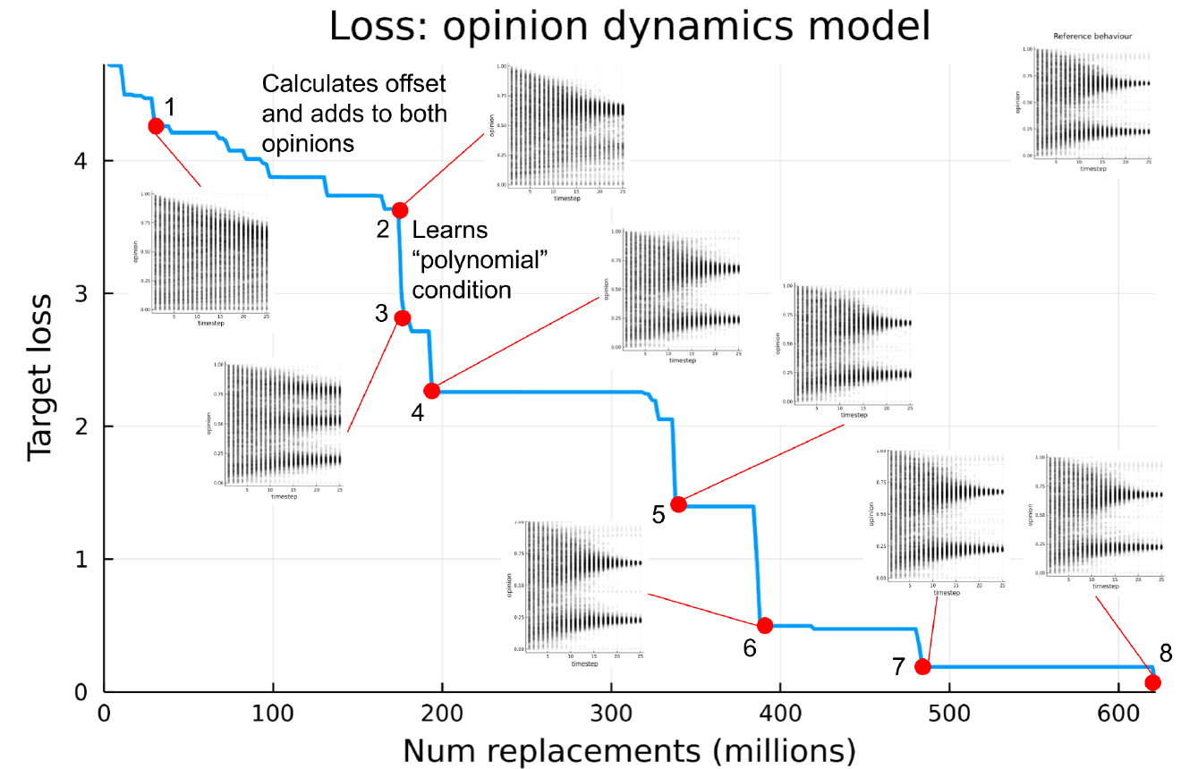
Figure 9 shows how the loss decreases over the course of the training run, with the outputs of running the best learned behaviour shown at transition points. There aren’t as many easily identifiable features of the model as with the flocking model, however we can still identify particular features by observing the model output and the generated code itself. By point 2 in Figure 9 the model has learned to calculate some offset and add this to both opinions, so that both opinions are update. After this there is a large transition between points 2 and 3, which corresponds to the model learning to calculate the polynomial function of the difference in opinion, which is a similar structure it uses for the rest of the training run. Once the loss decreases to around 2.0, at point 4, the model output is already subjectively very similar to the reference behaviour (the reference behaviour output can be seen in the top right hand corner of Figure 9). The loss continues to decrease after this point, although retaining the "polynomial" structure in the code and with subjectively similar output. It seems that it is just refining this structure and further tuning the numerical parameter values to more closely recreate the reference data. It is also worth noting that the plots in Figure 9 were produced using the same initial opinion values as the original reference data used in training, so although it is able to subjectively match the reference model output fairly early in the training run, it could be that it continues to improve its ability to generalise to other starting configurations, by matching the reference behaviour more closely, rather than over-fitting to the training data.
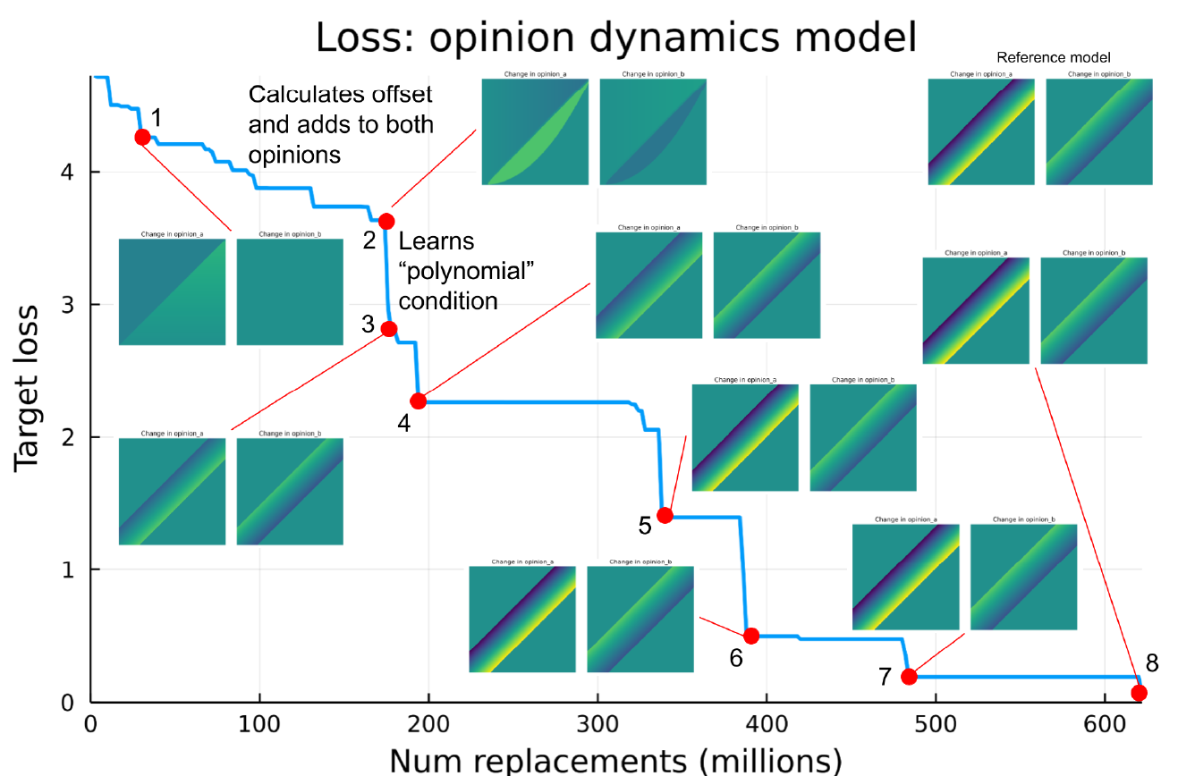
The opinion dynamics model has a useful property that lets us create an additional visualisation; the learned behaviour only has two inputs (the current opinions) and two outputs (the next opinions), and all of these values should be between 0.0 and 1.0 (although note that this range is not a hard constraint of the training process and theoretically the learned behaviours could output any value). This means we can plot a 2D map of all output values for every possible input value between 0.0 and 1.0 for both inputs, and display this as two 2D images side by side (one for each output). This provides a quick and visual way to characterise the full response of the behaviour to all valid inputs, without having to look at and understand the generated code itself. Figure 10 shows the loss plot for the same training run as Figure 9, however in this case the plots at each transition point show the “input/output” map image for all possible inputs for intermediate behaviours, instead of showing the output of running the learned behaviour as part of the agent-based model. Each plot shows two images, the left side represents the output \(opinion\_a\) and the right side \(opinion\_b\). Technically this shows the difference in opinion compared to the input value, rather than the output itself, so it is how much the function is changing the opinion of this agent. This can be thought of as a way of visualising only the learned behaviour function by itself, rather than the output of the full model, which is dependent on other things such as the initial opinion values of all agents and which agents are chosen randomly to interact with each other. This provides another way to see how the behaviour changes and improves over the training run. At point 1 in figure 10 the behaviour is only updating the first output, \(opinion\_a\), but not \(opinion\_b\), this can be seen in the left hand image in the plot at point 1 which represents the output \(opinion\_a\), the opinion is changed depending on the input values, however the right side representing \(opinion\_b\) is constant, which means it is unchanged by the function. This is because the behaviour hasn’t learned to apply an offset to both outputs yet.
At point two it can be seen that it is applying a change to both outputs, since both the left and right images show a pattern of difference that is dependent on the inputs. There is a curved shape near the center, which shows that the difference in opinion is greater when the input opinions are closer together (since it is close to the line \(x=y\)). As a reminder the reference model only updates the output opinions when the input opinions are within a threshold of each other.
By point 3 it has learned the “polynomial” logic, creating a similar threshold logic to the reference model, which can be seen in the input/output plot, since there is a narrow band in each plot parallel to the line \(x=y\), corresponding to a constant threshold. Note that the colours are different on either side of the band, which represents the offset needed to push the output opinion towards the center of the band, i.e. pushing the two opinions closer together, and therefore closer to the \(x=y\) line. Therefore point 3 seems to be where it recreates the correct threshold logic of the reference model, however the magnitude of the difference (represented by the colour) is not exactly the same as the reference model. This is because the reference model is actually asymmetric, and updates \(opinion\_a\) twice as much as opinion b. At point 5 it learns this asymmetry, and the input/output map now looks very similar to the one for the reference model, which can be seen in the top right corner of the figure. This input/output map has therefore revealed the point at which the model learns this feature, which wasn’t apparent from Figure 9, since the plotted model output looks subjectively similar at every transition after point 4.
Analysis of multiple training runs
A further 10 repetitions of the opinion dynamics experiment were conducted with the same configuration. Figure 11 shows how the loss decreases over all 10 training runs.
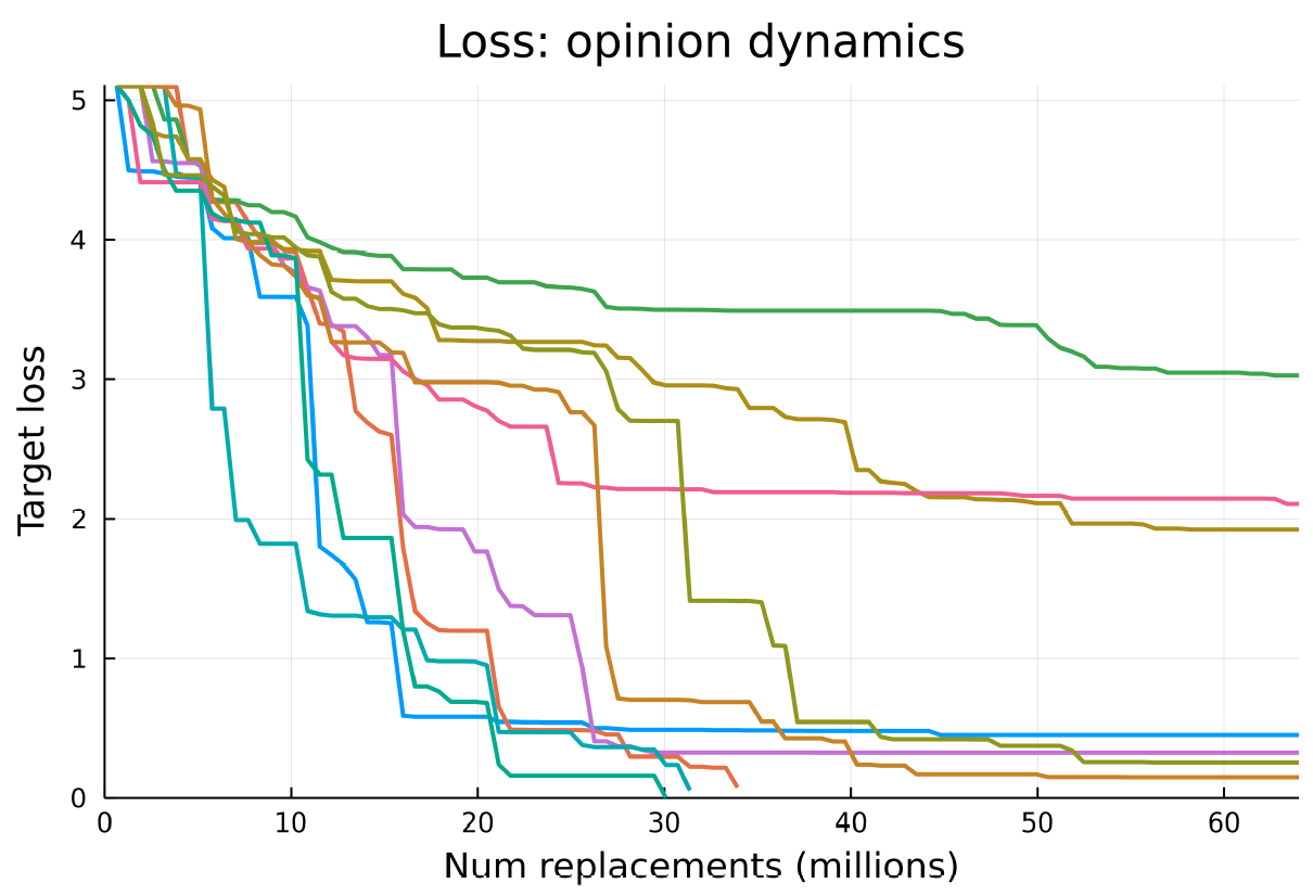
Unlike the flocking repetitions, not all of these opinion dynamics runs successfully perform well, three of the runs appear to get stuck in local minima and their loss does not decrease any further for reasons we do not fully understand but likely related to the roughness of the problemś landscape. The successful runs take around 7-10 hours (wall clock time on a n2d-highcpu-128 Google Cloud Instance) to reach convergence.
Most learned behaviours are relatively long with some complicated conditional logic, which makes them more challenging to interpret. Transitions seem to involve some rearrangement or refinement of this logic or numerical values, so it is harder to pick out clear features that have changed.
A key feature of the reference model logic is calculating the difference between the input opinions, then using this difference to determine whether to update the opinions or not. This difference can be denoted \(delta\_opinion\), which is the difference between the inputs \(opinion\_a\) and \(opinion\_b\). The absolute value of this difference can be obtained by using the \(abs\) function or by squaring. All the successful training runs consistently learn a behaviour which calculates this \(delta\_opinion\) within the first few lines of generated code, however the unsuccessful ones that fail to converge are all missing this important features.
Some of the training runs produced relatively short learned behaviours, such as the one shown in Listing 11, which achieves a loss of 0.07027 and is only 10 lines long after being automatically simplified. It is still not trivial to interpret the logic, however we can see that it is calculating \(delta\_opinion\), then applying an update to each output opinion conditional on this value.
function update_opinions(opinion_a, opinion_b)
	i = 1.1650 * ( opinion_b - opinion_a )
	p = ( i / 34.2139 * 1.4181 ) / 0.9178
	c = 0.2934 / i
	q = if less_than( 1.2694, scalar_abs( p + c ) )
		i * 0.2934
	else
		p
	end
	h = q - p
	return opinion_a + h * 1.7438, opinion_b - 0.8424 * h
endOne training run achieves a loss of , which is effectively zero difference between the output of this learned behaviour and the reference behaviour, i.e. it is a global maximum. The simplified code for this behaviour is shown in Listing 12. It is worth noting the last line where it calculates the outputs to return as \(q + q + opinion\_a\) and \(opinion\_b - q\), this is exactly the same logic as the reference behaviour, where it calculates an offset (here \(q\)) and applies double the offset to \(opinion\_a\).
function update_opinions(opinion_a, opinion_b)
	h = opinion_b - opinion_a
	if greater_than( 21750.4850, opinion_a )
		a = reciprocal( h )
		n = opinion_a + 14453413286210818048.0000
		c = 24.9944
	else
		a = 0.0000
		n = h
		c = 25.0249
	end
	o = square( a )
	b = o + o
	e = if less_than( c, o )
		b + b
	else
		n
	end
	q = a / e
	return q + q + opinion_a, opinion_b - q
endAnother point worth noting in comparison to the original training run is that most of the learned behaviours do not seem to learn the same "polynomial" approach, i.e. they do not use higher order powers of \(delta\_opinion\) in their calculations. So it seems as if there is nothing necessary about learning this feature, and there are other paths for the training process to learn alternative logic.
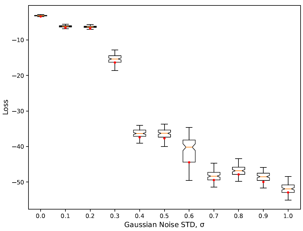
Generalisation
In order to assess the robustness of the best evolved solution we follow the same procedure we already employed in Section 5. Results are also similar to the ones of the flocking model and are shown in Figure 12. Like in the flocking model, the best evolved behaviour is very robust when evaluated against new 1000 unseen trajectories of the reference model (\(\sigma=0\) in Figure 12). In this case the variance in the loss with perfect training data appears to be even lower than in the flocking model. We also get similar performance when we inject increasing levels of Gaussian noise in the training set and re-train the model. Still we observe two sudden decreases in the loss with \(\sigma=0.3\) and \(\sigma=0.6\). In the latter the decrease in the loss is accompanied with a significant and momentary increase of the variance. We speculate that both sudden decreases in the loss correspond to the algorithm being unable to learn fundamental features of the model due to excessive noise in the training data — i.e., lack of information. The increase in variance when \(\sigma=0.6\) is consistent with a transition where the algorithm can still learn the fundamental feature in some trajectories but not in others, hence the increase and the following drop of the loss. Interestingly we also observe a moderate bump of the loss with \(\sigma=0.8\). This is suggestive that at the local level some noise can indeed increase the robustness of the solutions.
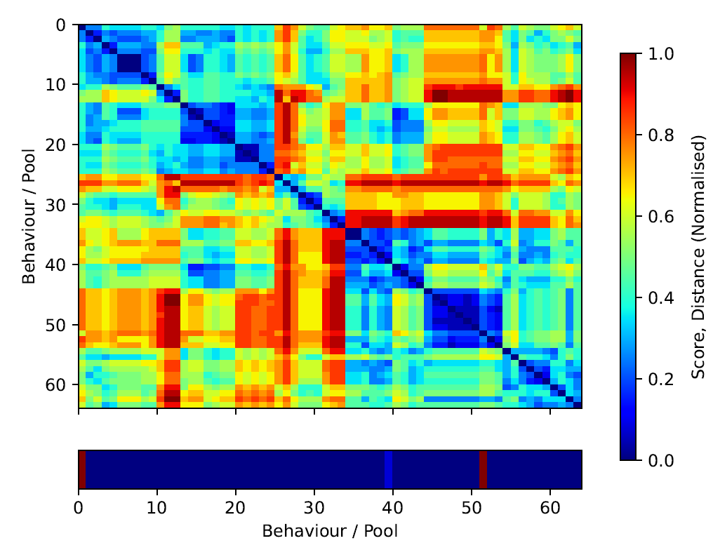
Population level analysis
We performed the same type of analysis we already did for the flocking model in Section 4.28. We compute the Hamming distance of the best candidate behaviours of each one of the pools in the last generation of a training run and construct a distance matrix. To help us understand the structure of the distance landscape we re-order the matrix to cluster similar behaviours together. Results in Figure 13 show that overall diversity of the population is significantly smaller with bigger cluster of similar sub-populations. This is likely a consequence of the reduced space of possible solutions compared to the flocking model. Still, we can observe two different high fitted sub-populations that provide different solutions — indices 0 and 51 in Figure 13. However, despite the solutions at a syntax-program level are indeed different (see 13 and 14 for the raw listings of both behaviours), our preliminary analysis of the programs once simplified show that both programs are actually the same. This is also consistent with the lack of diversity of loss scores in the population (there are just 4 different loss values) which are a proxy of genetic diversity. Given previous the previous analysis in Section 5.10, we know there are other high performing solutions that follow a different strategy, i.e., the "weird" polynomial function found in 5.10. We conclude that in this particular realisation of the opinion dynamics model the genetic algorithm gets stuck in a local maxima.
// Candidate Behaviour with index 0 and loss -0.003192596
function evaluate(opinion_a, opinion_b)
	divide_10 = ( opinion_b - opinion_a ) / 0.8263895926584304
	conditional_25 = if ( isapprox(0.2410781731936723, divide_10, atol=0.001) )
		scalar_abs( 3.835283665828663 )
	else
		scalar_clamp( 0.2410781731936723 )
	end
	conditional_28 = if greater_than( conditional_25, divide_10 )
		divide_10 * -15.619389770587324
	else
		0.0
	end
	mult_5 = opinion_a * opinion_b
	conditional_16 = if less_than( 0.2410781731936723, mult_5 )
		reciprocal( 2.2058532109510067 )
	else
		mult_5
	end
	mult_1 = 0.8263895926584304 * 0.2410781731936723
	minus_2 = opinion_a - mult_1
	conditional_17 = if greater_than( 0.8263895926584304, opinion_a )
		conditional_16
	else
		minus_2
	end
	conditional_18 = if ( isapprox(opinion_b, minus_2, atol=0.001) )
		conditional_17
	else
		minus_2
	end
	if greater_than( opinion_b, conditional_18 )
		conditional_29 = divide_10
		conditional_31 = conditional_28
		conditional_30 = conditional_25
	else
		conditional_29 = mult_1
		conditional_31 = 0.0
		conditional_30 = conditional_18
	end
	divide_16 = conditional_31 / -37.78048979189104
	plus_18 = divide_16 + opinion_a
	minus_19 = -15.619389770587324 - plus_18
	return plus_18, opinion_b - divide_16
end
// Candidate Behaviour with index 51 and loss -0.003192596
function evaluate(opinion_a, opinion_b)
	scalar_clamp_12 = scalar_clamp( 0.2410781731936723 )
	divide_11 = ( opinion_b - opinion_a ) / 0.8263895926584304
	conditional_26 = if ( isapprox(scalar_clamp_12, divide_11, atol=0.001) )
		scalar_abs( -37.78048979189104 )
	else
		scalar_clamp_12
	end
	conditional_29 = if greater_than( conditional_26, divide_11 )
		divide_11 * -15.619389770587324
	else
		0.0
	end
	mult_5 = opinion_a * opinion_b
	conditional_16 = if less_than( 0.2410781731936723, mult_5 )
		reciprocal( 2.2058532109510067 )
	else
		mult_5
	end
	minus_2 = opinion_a - 0.8263895926584304 * 0.2410781731936723
	conditional_17 = if greater_than( 0.8263895926584304, opinion_a )
		conditional_16
	else
		minus_2
	end
	conditional_18 = if ( isapprox(opinion_b, minus_2, atol=0.001) )
		conditional_17
	else
		minus_2
	end
	if greater_than( opinion_b, conditional_18 )
		conditional_32 = conditional_29
		conditional_31 = conditional_26
		conditional_30 = divide_11
	else
		conditional_32 = 0.0
		conditional_31 = conditional_18
		conditional_30 = square( opinion_b )
	end
	reciprocal_18 = reciprocal( -37.78048979189104 )
	divide_17 = conditional_32 / -37.78048979189104
	return divide_17 + opinion_a, opinion_b - divide_17
endPenalising complexity of learned behaviours
Generating interpretable model logic is key to achieving the goals of Inverse Generative Social Science (Vu et al. 2019), as we want to be able to understand new agent dynamics learned automatically from observed data. However the genetic algorithm has the tendency to produce somewhat over-complicated code. It was shown that this code can be interpreted with some effort, and to some extent this can be automatically simplified by manipulating the computational graph, however often the logic cannot be reduced further and it is a challenge to understand even the simplified generated model logic. Particularly in the case of opinion dynamics the genetic algorithm seems to generate more IF conditions than are strictly necessary to re-create the reference behaviour.
It would be beneficial to be able to further incentivise the genetic algorithm to produce less bloated behaviours but with similar loss values. Vu et al. (2019) take the approach of using multi-objective search, however in this case given the large number of model evaluations required to learn models from scratch it may be prohibitively expensive to use multiple separate objective criteria. The learning process is very sensitive to the choice of objective function and changing the objective function can prevent its ability to discover useful behaviours.
Experiments were conducted to add a complexity penalty to the existing loss function. Instead of multi-objective search with separate fitness functions, this complexity penalty was linearly combined with the existing loss term to provide a single fitness function. The complexity penalty was taken as the square of the length of the behaviour, and multiplied by a parameter \(\alpha\) to control the magnitude of the penalty. The resulting combined fitness function is then given as:
| \[f(behaviour) = loss(behaviour) + \alpha * length(behaviour)^2\] | \[(6)\] |
It is worth noting that the training process has a maximum behaviour length for each experiment, which is 28 lines for flocking and 20 lines for opinion dynamics. The mutation operator is also biased towards removing lines more often than it adds them (Greig & Arranz 2021), so the training process should already incentivise shorter behaviours to some extent. However the additional complexity penalty should further penalise long behaviours and guide the genetic algorithm towards shorter behaviours with equivalent loss.
A quadratic penalty was used because this will have proportionally less effect for shorter behaviours than for longer behaviours, since it is preferable to avoid changing the loss function too much for shorter behaviours, which may risk harming learning progress.
To allow the training process to make unimpeded progress early in the run, the complexity penalty was only introduced into the loss function once the loss gets below a certain threshold, which was set to a given value for both the flocking and opinion dynamics experiments, detailed below.
The first attempt at this experiment used the total length of the learned behaviours for the complexity penalty, however it was found that this completely halts training progress as soon as the complexity penalty is introduced, and the loss does not decrease any further beyond this threshold. It was hypothesised that this results in the training process removing any nonfunctional code which doesn’t affect the output, which means there is no redundant code to provide “raw material” for beneficial mutations later in the training run. To test this hypothesis, the complexity penalty was changed to use the logical length of the behavior, meaning only counting the instructions which affect the output of the behavior, and not counting redundant instructions. This means the training process is able to keep redundant instructions which can form the basis of beneficial mutations. These redundant instructions can then be stripped out at the end of the training process to provide shorter, more interpretable behaviours. Using this logical length complexity penalty greatly improved performance over the original complexity penalty, and allowed the training progress to go past the complexity penalty threshold and achieve a low losses. Experiments were conducted to find optimal values of the alpha parameter for both flocking and opinion dynamics, the results are given below. All results shown are using the logical length complexity penalty.
Complexity penalty results
Flocking
New training runs were conducted with the flocking model with a complexity penalty term in the fitness function with the following values of \(\alpha\): \([0.00005, 0.00015, 0.0001, 0.0002, 0.0005]\). The complexity penalty was only introduced when the loss went below a threshold of 100.0. All training runs were able to achieve a low loss apart from the run with the highest value of alpha, 0.0005, which stalled at a loss of 87.853, just below the threshold of 100.0. So it seems that higher complexity penalties do seem to inhibit evolution. However there was no clear trend of the complexity penalty reducing the logical length of the resulting behaviours, as can be seen in figure 14, which shows how the logical length varies over the training run as the loss decreases. Runs with a higher \(\alpha\) do not seem to achieve a shorter logical length. Overall, it appears that the introduction of a complexity penalty in the flocking model does not reduce the complexity of the behaviours. A further analysis shall be performed in order to determine why this is happening and possibly employ a different penalty function.
Opinion Dynamics
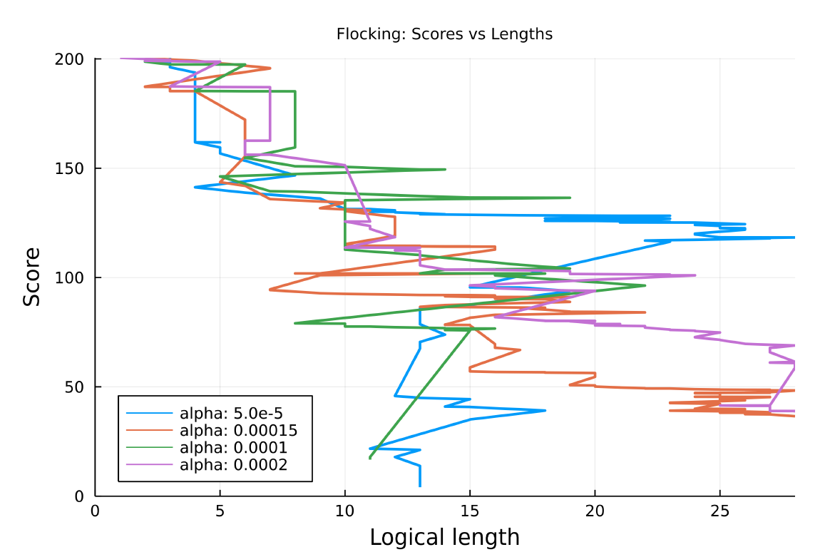
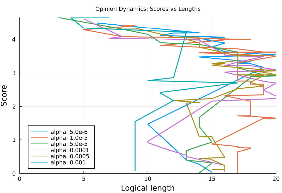
For the opinion dynamics model training runs were conducted with the following values of complexity penalty \(\alpha\): \([0.000001, 0.000005, 0.00005, 0.00001, 0.0001, 0.0005, 0.001, 0.05, 0.01]\). The complexity penalty was only introduced when the loss went below a threshold of 2.5.
Several runs got stuck in a local optimum and did not achieve a low loss, this happened for alpha values of 0.000001, 0.0005 and 0.001. Figure 15 shows how the logical length varies over the training run as the loss decreases, only the runs which successfully achieved a low loss are shown. The run with the highest alpha value (0.001) which successfully completed ends up with a significantly shorter best behaviour, with a logical length of 9, it also seems to maintain a consistently shorter best behaviour throughout the training run.
Higher values of \(\alpha\) appear to hinder the algorithm’s ability to identify efficient behaviors. For \(\alpha = 0.01\), the highest value, the loss stalls at exactly 2.5, which is the threshold for when the complexity penalty is introduced, implying that the complexity penalty is preventing further progress as soon as it is introduced.
A value of \(\alpha = 0.001\) appears to be close to optimal. Unlike the flocking experiment a complexity penalty with this value does seem to successfully encourage shorter learned behaviours.
Discussion and Conclusion
In this paper, we have demonstrated the potential of PS and GP for learning full symbolic representations of core model logic. By providing reference data and employing a flexible DSL consisting of domain-independent primitives without reliance on encoding existing domain knowledge, we further the goals of iGSS. This approach enables exploration of a larger space of possible model dynamics without being restricted by human preconceptions, especially important in areas such as social dynamics, where underlying mechanisms are often not well understood.
We successfully synthesized models in multiple domains, including opinion dynamics and flocking. In both cases, the resulting models were able to display nearly identical macro behaviors to our reference models. We demonstrated that the evolved behaviors generalize well and quantified their robustness to noise in the training data. Our population-level analysis of the final generations revealed that multiple high-performing solutions evolved, with some implementing very different strategies. Some of them seem unlikely to be designed by a human modeler, illustrating that the inverse generative approach can discover rules that might not easily occur to a human.
The learned behaviors’ logic can be partially interpreted and understood, thanks to the genetic algorithm mutation being biased towards shorter behaviors. We explored other methods of improving interpretability, such as adding a complexity penalty to the loss function based on the logical length of non-redundant instructions in the behavior. This approach effectively reduced the length of learned behaviors in opinion dynamics but not in the flocking experiment. Further analysis will be require to determine why.
Interpretability of behaviors allows for the analysis of intermediate behaviors during training runs, highlighting "transition points" with significant decreases in loss and identifying specific model features learned during these transitions. However, the interpretability of the resulting learned models varies. In particular, the opinion dynamics experiment tends to learn overly complicated conditional branching structures. Some training runs produced shorter behaviors, indicating that it is possible to learn succinct models and suggesting future attempts to guide the process towards simpler behavior code.
Several avenues for enhancing interpretability warrant further exploration. These include alternative measures of program "complexity" beyond simple program length, such as graph-based measures applied to the computational graph, or penalties for specific DSL operations, such as penalizing the use of too many conditional operators. We have a method for automatically simplifying behaviors using a graph representation; periodically applying this method inside the training loop could help maintain short, interpretable behaviors.
Another challenge lies in maintaining the diversity of the candidate population while still penalizing program bloating. Approaches inspired by novelty search (Lehman & Stanley 2011) could address this challenge, requiring a measure of behavior novelty instead of only its loss value calculated from the reference data. This criterion is potentially valuable in the context of iGSS, as it would force the search process to explore a broader diversity of possible mechanisms for explaining real-world phenomena. Furthermore, recent advances in foundation models (FM) based on Transformer architectures have demonstrated remarkable abilities to distill latent spaces from vast amounts of data. While most research has focused on linguistic data, FMs have proven equally powerful when trained or fine-tuned with program code (e.g., OpenAI Codex (Chen et al. 2021) and DeepMind’s AlphaCode (Li et al. 2022)) and have even been applied to PS (Austin et al. 2021). Such an approach could provide an efficient mechanism for directing the evolutionary process towards areas of the parameter space likely to contain solutions, potentially leading to powerful GP/PS approaches using general-purpose languages (e.g., Julia, Python, C, etc.) instead of DSLs.
References
ARRANZ, J., Noble, J., & Silverman, E. (2011). The origins of communication revisited. Available at: https://eprints.soton.ac.uk/197755/1/ARRANZ.pdf
AUSTIN, J., Odena, A., Nye, M., Bosma, M., Michalewski, H., Dohan, D., Jiang, E., Cai, C. J., Terry, M., Le, Q. V., & Sutton, C. (2021). Program synthesis with large language models. CoRR, Abs/2108.07732. https://arxiv.org/abs/2108.07732
BEZANSON, J., Edelman, A., Karpinski, S., & Shah, V. B. (2017). Julia: A fresh approach to numerical computing. SIAM Review, 59(1), 65–98. [doi:10.1137/141000671]
CHEN, M., Tworek, J., Jun, H., Yuan, Q., Pinto, H. P. d. O., Kaplan, J., Edwards, H., Burda, Y., Joseph, N., Brockman, G., Ray, A., Puri, R., Krueger, G., Petrov, M., Khlaaf, H., Sastry, G., Mishkin, P., Chan, B., Gray, S., Ryder, N., Pavlov, M., Power, A., Kaiser, L., Bavarian, M., Winter, C., Tillet, P., Such, F. P., Cummings, D., Plappert, M., Chantzis, F., Barnes, E., Herbert-Voss, A., Guss, W. H., Nichol, A., Paino, A., Tezak, N., Tang, J., Babuschkin, I., Balaji, S., Jain, S., Saunders, W., Hesse, C., Carr, A. N., Leike, J., Achiam, J., Misra, V., Morikawa, E., Radford, A., Knight, M., Brundage, M., Murati, M., Mayer, K., Welinder, P., McGrew, B., Amodei, D., McCandlish, S., Sutskever, I. & Zaremba, W. (2021). Evaluating large language models trained on code. arXiv preprint. Available at: https://arxiv.org/abs/2107.03374
DAVID, C., & Kroening, D. (2017). Program synthesis: Challenges and opportunities. Philosophical Transactions of the Royal Society A: Mathematical, Physical and Engineering Sciences, 375(2104), 20150403. [doi:10.1098/rsta.2015.0403]
DEFFUANT, G., Neau, D., Amblard, F., & Weisbuch, G. (2000). Mixing beliefs among interacting agents. Advances in Complex Systems, 3, 87–98. [doi:10.1142/s0219525900000078]
ELDREDGE, N., & Gould, S. (1971). Punctuated equilibria: An alternative to phyletic gradualism. Models in Paleobiology, 82, 82–115. [doi:10.5531/sd.paleo.7]
GOLDBERG, D. E., & Deb, K. (1991). A comparative analysis of selection schemes used in genetic algorithms. In G. Rawlins (Ed.), Foundations of Genetic Algorithms (Vol. 1, pp. 69–93). Amsterdam: Elsevier. [doi:10.1016/b978-0-08-050684-5.50008-2]
GONÇALVES, I., & Silva, S. (2011). Experiments on controlling overfitting in genetic programming. 15th Portuguese Conference on Artificial Intelligence (EPIA 2011)
GONÇALVES, I., Silva, S., Melo, J. B., & Carreiras, J. M. (2012). Random sampling technique for overfitting control in genetic programming. European Conference on Genetic Programming
GREIG, R., & Arranz, J. (2021). Generating agent based models from scratch with genetic programming. ALIFE 2021: The 2021 Conference on Artificial Life. Available at: https://direct.mit.edu/isal/proceedings/isal/64/102955 [doi:10.1162/isal_a_00383]
GULWANI, S., Polozov, O., & Singh, R. (2017). Program synthesis. Foundations and Trends in Programming Languages, 4(1–2), 1–119. [doi:10.1561/2500000010]
GUNARATNE, C., & Garibay, I. (2017). Alternate social theory discovery using genetic programming: Towards better understanding the artificial Anasazi. Proceedings of the Genetic and Evolutionary Computation Conference, New York, NY, USA [doi:10.1145/3071178.3071332]
HUSSELMANN, A. (2015). Generating opinion agent-based models by structural optimisation. COGNITIVE 2015: The Seventh International Conference on Advanced Cognitive Technologies and Applications, Nice, France
JUNGES, R., & Klügl, F. (2011). Evolution for modeling: A genetic programming framework for Sesam. Proceedings of the 13th Annual Conference Companion on Genetic and Evolutionary Computation, New York, NY, USA [doi:10.1145/2001858.2002047]
KOZA, J. R. (1992). Genetic Programming: On the Programming of Computers by Means of Natural Selection. Cambridge, MA: MIT Press.
KOZA, J. R. (1993). Evolution of emergent cooperative behavior using genetic programming. Computing with Biological Metaphors
LANGDON, W. (2011). Minimising testing in genetic programming. RN, 11(10), 1.
LEHMAN, J., & Stanley, K. O. (2011). Abandoning objectives: Evolution through the search for novelty alone. Evolutionary Computation, 19(2), 189–223. [doi:10.1162/evco_a_00025]
LI, Y., Choi, D., Chung, J., Kushman, N., Schrittwieser, J., Leblond, R., Eccles, T., Keeling, J., Gimeno, F., Dal Lago, A., Hubert, T., Choy, C., P. de Masson d’Autume, Babuschkin, I., Chen, X., Huang, P. S., Welbl, J., Gowal, S., Cherepanov, A., Molloy, J., Mankowitz, D. J., Sutherland Robson, E., Kohli, P., de Freitas, N., Kavukcuoglu, K. & Vinyals, O. (2022). Competition-level code generation with AlphaCode. arXiv preprint. Available at: https://arxiv.org/abs/2203.07814 [doi:10.1126/science.abq1158]
MANNA, Z., & Waldinger, R. J. (1971). Toward automatic program synthesis. Communications of the ACM, 14(3), 151–165. [doi:10.1145/362566.362568]
QUINN, M. (2001). Evolving communication without dedicated communication channels. European Conference on Artificial Life. Available at: https://link.springer.com/book/10.1007/3-540-44811-X [doi:10.1007/3-540-44811-x_38]
REAL, E., Aggarwal, A., Huang, Y., & Le, Q. V. (2019). Regularized evolution for image classifier architecture search. Proceedings of the AAAI Conference on Artificial Intelligence. [doi:10.1609/aaai.v33i01.33014780]
REAL, E., Liang, C., So, D. R., & Le, Q. V. (2020). AutoML-Zero: Evolving machine learning algorithms from scratch. arXiv preprint. Available at: https://arxiv.org/pdf/2003.03384.pdf
REYNOLDS, C. W. (1987). Flocks, herds, and schools: A distributed behavioral model. SIGGRAPH ’87 Conference Proceedings [doi:10.1145/37401.37406]
SHIN, R., Allamanis, M., Brockschmidt, M., & Polozov, O. (2019). Program synthesis and semantic parsing with learned code idioms. NeurIPS. Available at: https://proceedings.neurips.cc/paper_files/paper/2019/file/cff34ad343b069ea6920464ad17d4bcf-Paper.pdf
SMITH, V. A. (2008). Evolving an agent-based model to probe behavioral rules in flocks of cowbirds. ALIFE. Available at: https://synergy.st-andrews.ac.uk/vannesmithlab/files/2015/08/Smith_ALifeXI08_wErrata.pdf
STARKWEATHER, T., Whitley, D., & Mathias, K. (1990). Optimization using distributed genetic algorithms. International Conference on Parallel Problem Solving from Nature [doi:10.1007/bfb0029750]
VU, T. M., Probst, C., Epstein, J. M., Brennan, A., Strong, M., & Purshouse, R. C. (2019). Toward inverse generative social science using multi-objective genetic programming. Proceedings of the Genetic and Evolutionary Computation Conference, New York, NY, USA [doi:10.1145/3321707.3321840]
WOOLDRIDGE, M. (2009). An Introduction to Multiagent Systems. Hoboken, NJ: John Wiley & Sons.
WRIGHT, S. (1932). The roles of mutation, inbreeding, crossbreeding, and selection in evolution. Proceedings of the Sixth International Congress on Genetics. Available at: http://www.esp.org/books/6th-congress/facsimile/contents/6th-cong-p356-wright.pdf
ZHONG, J., Cai, W., Lees, M., & Luo, L. (2017). Automatic model construction for the behavior of human crowds. Applied Soft Computing, 56, 368–378. [doi:10.1016/j.asoc.2017.03.020]