Can Social Norms Explain Long-Term Trends in Alcohol Use? Insights from Inverse Generative Social Science

,
,
,
,
and
aUniversity of Sheffield, United Kingdom; bNew York University, United States; cThe Alan Turing Institute, United Kingdom
Journal of Artificial
Societies and Social Simulation 26 (2) 4
<https://www.jasss.org/26/2/4.html>
DOI: 10.18564/jasss.5077
Received: 15-Nov-2022 Accepted: 09-Mar-2023 Published: 31-Mar-2023
Abstract
Social psychological theory posits entities and mechanisms that attempt to explain observable differences in behavior. For example, dual process theory suggests that an agent's behavior is influenced by intentional (arising from reasoning involving attitudes and perceived norms) and unintentional (i.e., habitual) processes. In order to pass the generative sufficiency test as an explanation of alcohol use, we argue that the theory should be able to explain notable patterns in alcohol use that exist in the population, e.g., the distinct differences in drinking prevalence and average quantities consumed by males and females. In this study, we further develop and apply inverse generative social science (iGSS) methods to an existing agent-based model of dual process theory of alcohol use. Using iGSS, implemented within a multi-objective grammar-based genetic program, we search through the space of model structures to identify whether a single parsimonious model can best explain both male and female drinking, or whether separate and more complex models are needed. Focusing on alcohol use trends in New York State, we identify an interpretable model structure that achieves high goodness-of-fit for both male and female drinking patterns simultaneously, and which also validates successfully against reserved trend data. This structure offers a novel interpretation of the role of norms in formulating drinking intentions, but the structure's theoretical validity is questioned by its suggestion that individuals with low autonomy would act against perceived descriptive norms. Improved evidence on the distribution of autonomy in the population is needed to understand whether this finding is substantive or is a modeling artefact.Introduction
Motivation
Alcohol use is a major risk factor for non-communicable disease, contributing to 3 million premature deaths per year globally (World Health Organization 2018). The risks from alcohol use are not confined to people with alcohol use disorders (e.g., those ‘addicted’ to alcohol) but arise from even moderate levels of consumption. The epidemiology of alcohol is also complicated by the apparent protective effects of moderate consumption for some health conditions (e.g., coronary heart disease (Roerecke & Rehm 2010)) and also time lags between exposure and harm that can span multiple decades (Holmes et al. 2012). Monitoring and projecting how alcohol use is changing over time in a society is important for estimating how the consequent burden of harm to people’s health and healthcare services is likely to change, and to provide an impetus for policy action to try to reduce consumption levels and reduce harms.
In an evidence-based policy making environment, policy designers often make use of logic models to capture hypothesized causal pathways by which interventions are anticipated to have their effects. These pathways are scrutinized post-implementation in the evaluation phase (Craig et al. 2008). In the pre-implementation appraisal phase, computer modeling is increasingly used to estimate the impacts of alternative intervention options (Stewart & Smith 2015). To be compatible with the logic models, these computer models should encode transparent explanations for how interventions lead to changes in alcohol use in society—i.e., they should define structural assumptions about the social mechanisms driving change and stasis in alcohol use. Mechanism-based modeling generally, and agent-based modeling (ABM) specifically, is therefore well placed to make an effective contribution to alcohol policy appraisal and evaluation (McGill et al. 2021; Purshouse et al. 2021).
Using a generative approach (Epstein 1999, 2007), we can design and implement an ABM of candidate mechanisms and run the simulation to see if it can reproduce historical trends in population alcohol use—i.e., the so-called generative test. If the model passes the generative test then the mechanisms it encodes remain a candidate explanation that can, subsequently, be coupled to a logic model to forecast the impact of new interventions that are intertwined with the identified mechanisms. However, this result does not preclude other models being found that can also pass the generative test. In theory, there could be a multiplicity of surviving candidate models—a type of equifinality in the sense of multiple system processes, and multiple model structures and parameterizations, being able to reproduce the observed phenomenon to a similar degree (Beven 1993). Ideally, when making forecasts of policy effects, we would use an ensemble of such surviving models to provide the most robust estimates possible. In particular, if some models produce policy estimates with qualitatively different outcomes to others (i.e., more alcohol use, rather than less) then this would be important information for policy makers.
While modelers could in theory produce a number of different computational models for a given policy problem, due to practical constraints they tend to produce only one (although this may be subjected to sensitivity analysis around structural assumptions). However, machine learning methods open up the possibility of computational exploration of a space of ABMs and at least semi-automatic identification of a family of alternative models, including those not envisaged by a human modeler. Imagining such a concept in 1983, within a general modeling context, Openshaw (1983) described this model discovery approach as “model crunching”. Within an ABM context, Epstein (1999) discussed the possibility of searching across the space of agent rules, highlighting evolutionary computation as a promising means of efficiently searching the rule space. With machine learning methods now becoming more prominent, Epstein has led calls for a new era of model discovery for complex social simulations—what he has labelled as “inverse generative social science” (iGSS) (Epstein 2019)—and has now set out a manifesto for this nascent science (Epstein 2023).
Research aims
In earlier work, Buckley et al. (2022a) developed a hybrid theory-based model of alcohol use behaviors. The model aims to capture a dual process representation of agent cognition, where agent behaviors can be either intentional or habitual. The intentional process is based on the reasoned action theory known as the Theory of Planned Behavior (Ajzen 1991), which is a popular choice for social psychology experimental studies of alcohol use behaviors (Cooke et al. 2016). Buckley et al. (2022a) combined this cognitive model with norm theory—a sociological theory of how people both respond to and shape social norms, which has also been a focus for empirical studies in the alcohol use field (Keyes et al. 2012). The parameters of this hybrid model were then calibrated to a specific spatio-temporal setting: the US from the mid-1980s (the beginning of representative surveys capturing alcohol use in US society) to the mid-2010s. Six empirical time series targets were used for the calibration process: prevalence of alcohol use, mean frequency of alcohol use (drinking days per month), and mean quantity of alcohol use (grams of ethanol per day), with each measure split by sex (since drinking trends and risks of alcohol-related harm differ substantially for men and women). The best calibrated model was able to reproduce the prevalence and frequency targets successfully (including in an unseen portion of the time series used for validation), but struggled to provide a good fit to quantity targets—particular for men.
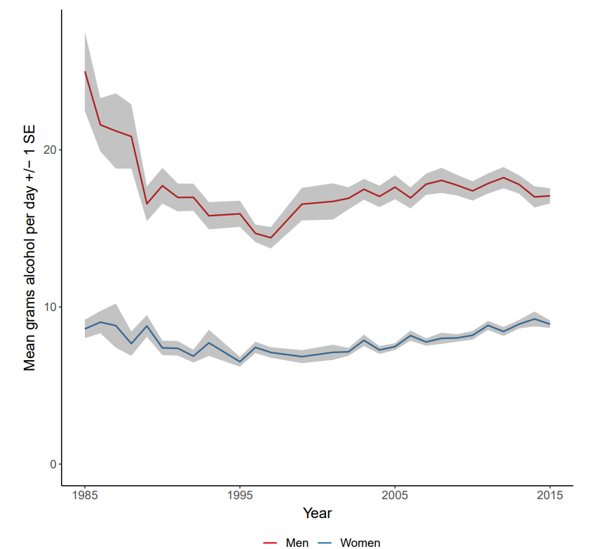
In the present study, within an iGSS framework, we explore whether alternative versions of Buckley et al. (2022a) model can provide an improved fit to the target data. Given that US-level alcohol use trends are relatively stable over the calibration window, we change to a setting with more interesting trend dynamics—the state of New York (Figure 1). New York has some of richest dynamics seen in per capita consumption, in comparison to other states. Motivated by a desire to understand deficiencies in the hybrid theory, we also investigate whether isolating the male and female targets produces different best-fitting candidate model structures. Since both dual process theory and norm theory are both intended to ‘explain away’ any variation in behavior by sex (or other variable-centric ‘determinants’ of alcohol use), differences in model structures between the sexes would indicate, and may help to identify the cause of, deficiencies in model design. In summary, the paper aims to address the following questions:
- Can a computational model drawing from dual process theory and norm theory generate the long-term alcohol use trends in New York from the mid-1980s to mid-2010s?
- Is there a single model that passes the generative test for both male and female trends simultaneously?
- What are the implications of the iGSS findings for computational modeling of health behaviors that draws on dual process theory and norm theory?
Background
Existing works in inverse generative social science
In pattern-oriented modeling (POM), multiple candidate ABM structures (each perhaps derived from alternative theories or representing different mechanisms) are tested for their ability to generate emergent phenomena (Grimm et al. 2005). The number of candidate models is typically small and constructed by hand. For example, in a recent POM study, Ge and colleagues enumerated 16 different model configurations that exhaustively tested combinations of including or excluding four different mechanisms driving trends in Scottish farming (Ge et al. 2018). In its standard form, POM does not consider any procedure for refinement or evolution of model structures; however Cottineau and colleagues introduced an incremental approach to ABM structural development, known as evaluation-based incremental modeling method (EBIMM), where mechanisms are gradually added and refined by the modeler in order to generate the target emergent phenomenon (Cottineau et al. 2015).
Where iGSS differs from POM and EBIMM is in the automation of ABM model structure construction and generative testing, enabling a systematized process that can explore the space of possible structures at a scale not feasible for a human modeler. All the existing approaches to iGSS, described below, use evolutionary algorithms to operationalize the search process. To our knowledge, the earliest study that could be recognized as an iGSS process is by Smith (2008), who used a genetic algorithm to evolve behavioral rules in an ABM of empirical association patterns in flocks of birds. The rules were classifier systems of fixed complexity, where the genotype of a candidate rule was a binary chromosome corresponding to different if-then options. Following Smith’s work, in the first study of a human social system, Zhong et al. (2014) identified discrete choice utility functions for pedestrians in order to reproduce emergent crowd patterns. Gene expression programming was used to evolve the utility functions, where the maximum complexity of the function is defined by the fixed chromosome length. While the ambition of this approach was to reproduce empirical crowding behavior, only simulated data was used in the study. In a sequence of studies, Gunaratne & Garibay (2017a), Gunaratne & Garibay (2017b), Gunaratne & Garibay (2020) used iGSS to identify candidate discrete choice utility functions for the seminal Artificial Anasazi model (Axtell et al. 2002). To our knowledge, the 2017 papers are the first iGSS studies of human behavioral rules using empirical target data. Genetic programming was used to operationalize the search, with model complexity handled by applying a constraint to the maximum tree depth of a genetic program. These studies are also notable in using data mining on candidate models arising from multiple runs of the iGSS process in order to identify commonalities in the components of the agents’ utility function. Gunaratne and colleagues’ evolutionary model discovery framework has also been applied to understanding the mechanisms of message prioritisation by social media users, using empirical data from social media platforms (Gunaratne et al. 2021).
Generative model discovery in the physical sciences has previously attempted to capture the potential trade-off between goodness-of-fit to empirical data and model complexity or parsimony; however here the generative models are typically differential equations representing physical systems rather than social processes (Schmidt & Lipson 2009). There is also an interesting seam of model discovery research in the physical sciences seeking to identify cellular automata rules and neighborhood structures, for both one-dimensional and two-dimensional topologies, from temporal slices of the evolution of the emergent spatio-temporal pattern (Richards et al. 1990). Here, the goodness-of-fit is measured via examining one-to-one correspondence between the individual automata responses and the target system, rather than through direct comparison of emergent structures. Some of these studies have also considered the trade-off between goodness-of-fit and structural parsimony, generating Pareto fronts using multi-objective evolutionary algorithms (Yang & Billings 2000).
Recent iGSS work has also aimed to capture such Pareto fronts through the use of multi-objective evolutionary algorithms. Vu et al. (2019) developed a method using multi-objective genetic programming (MOGP) with the two objectives of empirical goodness-of-fit and the number of nodes in the genetic program. The method was applied to a social norms model of alcohol use behaviors attempting to reproduce population trends in drinking in the US. The method was later extended to include a domain expert in the loop and to make use of multi-objective grammar-based genetic programming (MOGGP) (Vu et al. 2020a). The approach was used to discover alternative formulations of social role theory that could explain the US drinking trends, with explicit comparison to empirical findings within the domain literature on the varying contribution of social role factors. These methods are underpinned by a unifying mechanism-based social systems modeling (MBSSM) framework that allows modular ABM components to be integrated together (Vu et al. 2020b). This framework enabled iGSS to be used to study integrations of social norm theory and social role theory in determining how individuals make their next drinking decision within a drinking occasion (Vu et al. 2021).
Given that iGSS represents a new frontier in social simulation, there are many research challenges that remain to be addressed, including efficiency of the search process (e.g., through use of surrogate modeling), further integration of domain experts and data, and a more consistent approach to uncertainty quantification (e.g., the explicit consideration of prior probabilities for different mechanisms). There has also been little work done so far on how the choice of targets influences the iGSS findings and interpretations of the mechanisms so identified.
Existing agent-based models for alcohol policy appraisal
A recent scoping review by McGill et al. (2021) identified 25 ABM studies of alcohol-related behaviors. Here we elaborate on that review in terms of the theories represented by the model structures and the degree of empirical embeddedness of the models (Boero & Squazzoni 2005).
Theories represented
In all but one model, the agents represent individual people; in the remaining study (Spicer et al. 2012), the agents represent city blocks. Perhaps unsurprisingly for ABMs, a variety of the models focus on social influence processes arising from direct agent-to-agent interaction (Gorman et al. 2006; Ip et al. 2012; Jackson et al. 2012; Perez et al. 2012), although only two include contemporaneous social selection mechanisms (Giabbanelli & Crutzen 2013; Schuhmacher et al. 2014). The joint processes of niche theory and assortative drinking, proposed by Gruenewald (2007) have been adopted in at least two ABMs (Castillo-Carniglia et al. 2019; Fitzpatrick & Martinez 2012).
Social psychological theories are also represented: drinking motives are included in the model by Giabbanelli & Crutzen (2013), the theory of planned behavior forms the centerpiece of the model by Purshouse et al. (2014), Atkinson et al. (2018)'s ABM is informed by the capability-opportunity-motivation-behavior (COM-B) model.
Sociological theories are also represented: Fitzpatrick et al. (2015, 2016)'s models are based on social norms theory and social identity theory. The norm theory in these models relate to perceived descriptive norms; Probst et al. (2020) also base their model on norm theory, but include injunctive norms in addition to descriptive norms. Role theory is also represented in one of the ABMs (Vu et al. 2020b), for which an integrated design with norm theory is also shown (Vu et al. 2020a).
One further model blends different types of mechanisms together, using a causal loop diagram framing more usually associated with system dynamics modeling (Stankov et al. 2019). In a further seven models, the mechanisms encoded by the ABMs are not associated with any clear theoretical position (Garrison & Babcock 2009; Keyes et al. 2019; Lamy et al. 2011; Redfern et al. 2017; Scott et al. 2016a; Scott et al. 2016b; Scott et al. 2017).
Empirical embeddedness
Credibility of the model and trust in its outputs are critical to the usefulness of a policy appraisal model (Stewart & Smith 2015). In this context, ensuring an empirically rich parameterization of the model inputs and parameters—situating the policy in the specific time and place where it is being considered for implementation—is often regarded as important (Thiele et al. 2014). Of the 25 studies, 10 do not attempt any calibration to data, while a variety of different approaches to calibration can be found across the remaining 15 works.
Several studies initialize the agent population using survey data, often requiring the synthesis of several distinct data sources (Atkinson et al. 2018; Castillo-Carniglia et al. 2019; Fitzpatrick et al. 2016; Giabbanelli & Crutzen 2013; Keyes et al. 2019; Probst et al. 2020; Purshouse et al. 2014; Scott et al. 2016a; Scott et al. 2016b; Scott et al. 2017; Stankov et al. 2019; Vu et al. 2020b). A number of studies initialize the agent environment with data drawn from specific jurisdictions concerning the location of alcohol outlets (Castillo-Carniglia et al. 2019; Keyes et al. 2019; Redfern et al. 2017; Spicer et al. 2012; Stankov et al. 2019).
In terms of model parameter calibration, a number of studies make use of empirical target data (i.e., data that the ABM output can be compared to) to inform model parameters. In the related models by Castillo-Carniglia et al. (2019) and Keyes et al. (2019), model parameters are adjusted until model outputs (e.g., alcohol-related homicide rates) are similar to those of the target jurisdiction. These models also include a ‘burn in’ period of 110 time steps to allow for model outputs to stabilize, after which comparisons are made to static targets from a defined period (e.g., an estimate of the alcohol-related homicide rate in New York City in the early-to-mid 2000s). A similar approach is adopted by Perez et al. (2012), who run the model for 200 time steps and compare an average of the last five time steps to target data for a specific year.
While the above studies compare the equilibrium state of the ABM to static target data, other studies have attempted to reproduce dynamical trends in the target systems immediately following the defined initial conditions for the model (i.e., with no burn in). Stankov et al. (2019) compare model outputs to 5 year depression and alcohol misuse trends from survey data; Purshouse et al. (2014) compare to seven years of drinking frequency survey data; Probst et al. (2020) and Vu et al. (2020b) compare to six alcohol consumption targets for the 20 year period from 1979 to 1999. The latter study is notable as the only one of the 25 to calibrate the model structure (i.e., the agent rules) in addition to the model parameters.
Since calibration processes may overfit models to data (by capturing the noise in the data, in addition to the dynamics of interest), examining the performance of models over a separate validation data set is also regarded as good practice. This approach can also test other important assumptions for policy modeling, such as that the estimated model parameters are time-invariant (i.e., that the model estimates can be trusted outside of the immediate spatio-temporal context). Only two of the 25 models describe validation outcomes—a successful single year validation window in Purshouse et al. (2014) and an only partially successful 10 year validation window in Vu et al. (2020b). Systematic description of the calibration approach is also limited to just a few studies (Probst et al. 2020; Purshouse et al. 2014; Vu et al. 2020b).
Research gap
When considering the existing ABM studies of alcohol-related behaviors, there is a clear need for improved empirical embeddedness, not just in terms of parameter calibration, but also in terms of model structure selection and model validation. There also exists a need for a more systematic approach to empirical embedding. In the present study, we consider how iGSS can be used to address this research gap.
Alcohol Use Behaviors: Postulated Entities and Mechanisms
Model description
We use a computational model of drinking behaviors recently proposed by Buckley et al. (2022a). This model exploits the architecture developed by Vu et al. (2020b) that facilitates the application of iGSS methods (Vu et al. 2020a). The computational model is designed to be a modular mechanism that can be plugged in to broader dynamical models of alcohol use. We use a limited realization of the dynamics of the model in what follows. The agents in the model are individuals, and are assumed to be representative of adults in the US. Agent behaviors are typologized using five schema representing different daily drinking practices: abstaining, light drinking, moderate drinking, heavy drinking and very heavy drinking. While these schema are derived from an ordering based on number of drinks consumed, they are treated as unordered in the model.1 To introduce the cognitive processes that lead to the selection of a schema on a particular day by a particular individual, consider an example agent, Agent Alan. Our agent is endowed with two competing pathways: intentional action and habitual action. Agent Alan has an attribute, automaticity, that describes his tendency to follow the habitual rather than intentional pathway. Automaticity is defined continuously on the range \([0; 1]\), from always behaving intentionally to always behaving habitually, and varies between agents. In the present model, automaticity is a static attribute—it does not vary over time.
On every day of the simulation, the intentional or habitual process is triggered probabilistically for Agent Alan. Assuming that the habitual process is triggered, Agent Alan will randomly and without replacement select a schema from his history.2 The history represents the instances of schema performed by Agent Alan over the previous \(n\) days, excluding any instances that have already been selected through the habitual process. At the end of the \(n\) days, where the window \(n\) varies between agents, the history is refreshed with all the instances of schema performed over the previous window, regardless of whether they arose from the habitual or intentional pathway.
Assuming instead that the intentional pathway is triggered, we now consider three further attributes of Agent Alan: his attitude, subjective norms, and perceived behavioral control relating to each schema. Each of these attributes is defined for each schema (15 attributes in total3) over an unbounded continuous range, each representing a component of utility that contributes to the rational choice of intentionally selecting a schema. The net utility for a schema is a weighted sum of the attitude, subjective norms and perceived behavioral control corresponding to that schema. The weights are population-level parameters that are identical across agents, representing the universal relative importance of these attributes to the formation of intentions. In the present model, attitude is a static attribute, subjective norms is a dynamic attribute, and perceived behavioral control is assumed to be zero (i.e., it does not affect intention). Example values of these attributes for Agent Alan are shown in Table 1. Consider Agent Alan’s attitude toward abstaining: his attitude represents his personal evaluation of abstaining and is -1, indicating a negative evaluation. His subjective norms represents his perception of others’ behavior in relation to abstaining combined with his perception of society’s rules around abstaining; Agent Alan’s subjective norm is +2, indicating that he perceives abstaining as being encouraged by society. His perceived behavioral control represents his perceived ability to perform abstention; the value 0 indicates a neutral impact on intention. Assuming population weights of 0.5, 0.5 and 0 for attitudes, subjective norms, and perceived behavioral control respectively, his net utility of abstaining is +0.5. Similar utilities can be calculated for the other schema in Table 1. The utilities are converted to intentional probabilities using the standard discrete choice equation for multinomial log odds. When considered against the utilities for other schema, the probability that Agent Alan will choose to abstain is 0.33. Note that this probability is conditional on the intentional pathway having been triggered. If Agent Alan’s automaticity were 0.4, then the unconditional probability of abstaining would be a minimum of \(0.33\times(1-0.4)=0.20\) (and would be greater than this value if his history contained instances of abstaining that had not yet been sampled).
| Utility components | Intention | ||||
| Schema | Attitude | Subjective norms | Perceived behavioral control | Utility | Probability |
| Abstaining | -1 | +2 | 0 | +0.5 | 0.33 |
| Light drinking | +1 | +1 | 0 | +1 | 0.20 |
| Moderate drinking | +1 | 0 | 0 | +0.5 | 0.33 |
| Heavy drinking | +1 | -2 | 0 | -0.5 | 0.12 |
| Very heavy drinking | -1 | -4 | 0 | -2.5 | 0.02 |
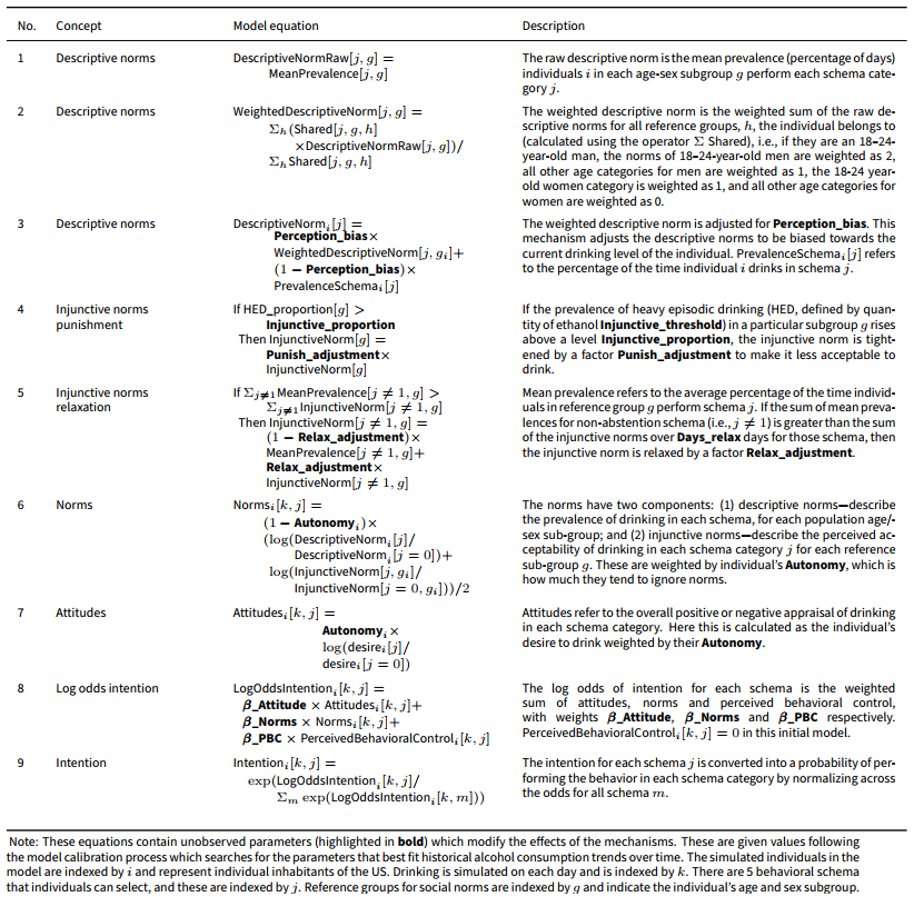
In the present model, Agent Alan’s only dynamically updating attribute is his subjective norms. The update mechanism is adapted from an existing computational model of social norms by Probst et al. (2020). Agent Alan is associated with a reference group based on his sex and age.4 The reference group is used to define two dynamic normative social structures: descriptive norms, which define the prevalence of schema instances currently performed by agents associated with each reference group, and injunctive norms which describe the current social acceptability of a person of that reference group performing each schema—the latter is defined continuously on the range \([0; 1]\) from performance of the schema is completely unacceptable to completely acceptable. Values for the injunctive norms for each age and sex reference group are initialized based on empirical data from the National Alcohol Surveys (NAS)5 on perceptions of the acceptability of drinking (Greenfield & Room 1997). Agent Alan updates his subjective norms through his perceptions of both the current descriptive and injunctive norms. His perception of the descriptive norms is affected by his own drinking, expressed as a weighted sum of his own schema prevalence and the reference group’s schema preference, where the weight is universal for all agents. For example, if Agent Alan is a heavy drinker, he will perceive the descriptive norms to be more positively skewed towards heavier drinking (i.e. assuming that others are also drinking heavily). The overall subjective norm is computed as the weighted average of the log-odds representation of the descriptive norm and injunctive norm. Finally the subjective norm is attenuated by a factor \((1-\textrm{autonomy})\), where \(\textrm{autonomy}\) is a static attribute of Agent Alan that represents the extent to which he ignores the influence of social norms. Autonomy is defined continuously on the range \([0; 1]\), from no autonomy to full autonomy, and varies between agents according to a calibrated distribution. Detailed descriptions of concepts and equations used to operationalize the intentional pathway are listed in Table 2.
The structural descriptive and injunctive norms are both dynamically updated for each reference group. The descriptive norm is a simple aggregation of schema performance by agents of the reference group. The injunctive norm is progressively adjusted by two mechanisms: (1) a so-called punishment mechanism that tightens the restrictiveness of the norms (i.e., moving them closer to zero) if the prevalence of heavy drinking by members of the reference group exceeds a threshold tolerance; (2) a relaxation mechanism that shifts the injunctive norms slightly closer to the current descriptive norms.
The computational model is implemented in C++ using the mechanism-based social systems modeling (MBSSM) software architecture (Vu et al. 2020b) and Repast HPC (Collier & North 2013). The source code of the model is available at: https://bitbucket.org/r01cascade/ge_norm_igss/
Model initialization
Agents are initialized using an existing microsimulation model (Brennan et al. 2020). This comprises a synthetic population of adults aged 18-80 representative of individuals in New York state between 1985 and 2015. The microsimulation integrates data on the US state level population from several sources including the US Census (Manson et al. 2019), American Community Survey (Ruggles et al. 2020) and accounts for population developments such as births, deaths and migration over time. Data from the Behavioral Risk Factor Surveillance System (BRFSS, Centers for Disease Control and Prevention (CDC) 2019) is used to initialize agents with baseline socio-demographic characteristics (including age and sex) and baseline alcohol consumption (12-month drinking status and usual quantity and frequency of drinking). Properties of the synthetic individuals, at baseline are shown in Table 3.
| Characteristic of the synthetic population | Initialization data |
|---|---|
| N agents | 1000 |
| Sex, % male | 43.7% |
| Age, mean years (SD) | 42.7 (16.7) |
| Non-drinker (%) | 18.9% |
| Mean grams per day among drinkers (SD) | 15.3 (26.5) |
| Mean drinking days per month among drinkers (SD) | 10.2 (9.3) |
Empirical calibration
Target data for calibration are taken from the US Behavioral Risk Factor Surveillance System (BRFSS) survey data for New York, adjusted to per capita New York State alcohol sales data for each year (Buckley et al. 2022a). Three alcohol use targets are defined for each year describing: (1) prevalence—the overall proportion of individuals consuming alcohol at least once during the previous year; (2) quantity—the average grams of ethanol consumed per day among drinkers; and (3) frequency—the average number of drinking days per month amongst drinkers. Targets are calculated separately for each year and split by sex. Models are calibrated using data for the years 1984-2010 and validated using reserved data from 2011–2015.
The original model was calibrated to targets for the US population as a whole and a fresh calibration to the New York State targets was required for the present work. The calibration process is a simple 1000 sample Latin hypercube over the model parameters, where the Latin hypercube design is optimized for its space-filling properties. Each individual is assigned a value of autonomy, automaticity and the \(n\) days over which to update drinking habits. These attributes are informed as part of the calibration process. For autonomy, values are taken from a beta distribution that is calibrated separately for males and females, and varies according to drinking patterns to allow for heavier drinkers and non-drinkers to be influenced differently by social norms. Automaticity is also represented by a calibrated beta distribution whereby low, medium and heavy drinkers have different distributions. The length of time habits take to update for an individual are represented by a calibrated truncated normal distribution, for which prior beliefs are informed by existing psychological research on habit formation (Lally et al. 2010). The calibration wrapper code and targets data are available at: https://bitbucket.org/r01cascade/calibration_jasss/
Model discovery methods
To search for the combinations of social theories that offer the best explanation to the macro-level phenomenon, we make use of multi-objective grammar-based genetic programming.
Genetic programming
Genetic programming (GP) (Koza 1992) is used to generate computer programs6 automatically with the help of genetic operators. It is usually applied to problems where there is an underlying requirement for structural optimization, besides the need (or not) to find the optimal parameters of the problem. An example is the design of a digital filter where besides having to find a set of optimal filter parameters, one also needs to determine the order of the filter. Although traditional genetic algorithms (GAs) are well suited for finding the optimal parameters of an optimization problem, they are not able to represent the structural requirements of a solution in chromosomes. A chromosome in GP, besides supporting constants, has provision for variables and functions (including algebraic operators, such as \(+\) and \(-\)), which can be combined in different ways to generate a syntax tree. In a similar fashion as it is done for GAs, a GP algorithm evolves a population of computer programs (or candidates) over many generations where selection and variation operators (e.g., crossover and mutation) take turns to find the fittest individuals. Traditionally in GP, Lisp prefix notation was used to represent a syntax tree in a chromosome but it has several shortcomings, such as the chromosome can have variable length, and that it is very easy for crossover and mutation operators to generate illegal (programmatically invalid) offspring. To mitigate these shortcomings, this paper uses grammatical evolution (GE) (O’Neill & Ryan 2001, 2003) which relies on the Backus–Naur form (BNF) syntax. This ensures chromosomes with a fixed length, restricts the search space in a way that it is possible to apply standard crossover and mutation operators more freely, and prevents the generation of illegal offspring.
Multi-objective optimization
In this study our interest is to find model structures and parameters that offer the best trade-offs between the complexity of the model and the goodness-of-fit with respect to multiple phenomenon targets. In total there are three objectives in this grammar-based genetic programming problem that have to be dealt with simultaneously, and these are: female alcohol use; male alcohol use, and complexity. When dealing with multiple conflicting objectives the problem does not contain a single optimal solution, which is often the case with single-objective problems. Besides the existence of a single optimal solution for each objective function, there is also a set of trade-off solutions where an improvement in one objective is earned at the expense (deterioration) of another objective(s). The best trade-offs in terms of Pareto optimality can be captured by the concept of dominance. Consider two solutions \(\mathbf{a}\in \mathcal{R}^M\) and \(\mathbf{b}\in \mathcal{R}^M\) where \(M\) is the number of objectives: \(\mathbf{a}\) is said to dominate \(\mathbf{b}\) if \(\mathbf{a}\) is not worse than \(\mathbf{b}\) in all objectives (i.e., \(a_i \leq b_i~ \forall i=1,\ldots,M\)), and \(\mathbf{a}\) is strictly better than \(\mathbf{b}\) in at least one objective (i.e., \(\exists_{i\in \{1,\ldots,M\}} : a_i < b_i\)). From a set of solutions, any subset that contains only solutions that are not dominated by any other solution in the set constitutes a non-dominated set, and the non-dominated set with respect to the entire search space is known as the Pareto optimal set.
We use the following objectives in this study. First we consider the overall goodness-of-fit between the model output and the target data, accounting for sampling uncertainty in both the output and target measurement. Here, our objective function for model structure \(\mathbf{x}\) is based on an implausibility metric (Vernon et al. 2010), \(I_{k,m}\), that measures the error between the \(m\)th simulated output \(y_m^\star\), averaged over \(N\) model runs of structure \(\mathbf{x}\) with different random number seeds \(n\), and equivalent empirical target data \(y_m\) over a sequence of temporal observations \(k\) defined by:
| \[ %z_1 = \frac{1}{KM}\sum_{k=1}^K\sum_{m=1}^M\frac{\left|\left(\frac{1}{N}\sum_{n=1}^Ny^\star_m[k]_n\right) - y_m[k]\right|}{\sqrt{(s_m[k])^2+(d_m)^2}} %z_1 = \max_{k,m}\left[\frac{\left|\left(\frac{1}{N}\sum_{n=1}^Ny^\star_m[k]_n\right) - y_m[k]\right|}{\sqrt{(s_m[k])^2+(d_m)^2}}\right] I_{k,m}(\mathbf{x}) = \frac{\left|\left(\frac{1}{N}\sum_{n=1}^Ny^\star_m(\mathbf{x}\mid n)[k]\right) - y_m[k]\right|}{\sqrt{(s_m[k])^2+(d_m)^2}},\] | \[(1)\] |
We define as an objective the maximum implausibility observed across all outputs \(m\) and all time points \(k\):
| \[ z_1(\mathbf{x}) = \max_{k\in \mathcal{K},m\in\mathcal{M}} I_{m,k}(\mathbf{x}),\] | \[(2)\] |
Since we are interested in whether the iGSS process might work better for male targets than female targets, and vice versa, we also decompose this first objective into two sub-objectives:
| \[ %z_{1,\textrm{male}} = \frac{1}{KM_{\textrm{male}}}\sum_{k=1}^K\sum_{m=1}^{M_{\textrm{male}}}\frac{\left|\left(\frac{1}{N}\sum_{n=1}^Ny^\star_m[k]_n\right) - y_m[k]\right|}{\sqrt{(s_m[k])^2+(d_m)^2}} %z_{1,\textrm{male}} = \max_{k,m\in M_\textrm{male}}\left[\frac{\left|\left(\frac{1}{N}\sum_{n=1}^Ny^\star_m[k]_n\right) - y_m[k]\right|}{\sqrt{(s_m[k])^2+(d_m)^2}}\right] z_{1,\textrm{male}}(\mathbf{x}) = \max_{k\in \mathcal{K},m\in\mathcal{M}_\textrm{male}} I_{m,k}(\mathbf{x}),\] | \[(3)\] |
| \[ %z_{1,\textrm{female}} = \frac{1}{KM_{\textrm{female}}}\sum_{k=1}^K\sum_{m=1}^{M_{\textrm{female}}}\frac{\left|\left(\frac{1}{N}\sum_{n=1}^Ny^\star_m[k]_n\right) - y_m[k]\right|}{\sqrt{(s_m[k])^2+(d_m)^2}} %z_{1,\textrm{female}} = \max_{k,m\in M_\textrm{female}}\left[\frac{\left|\left(\frac{1}{N}\sum_{n=1}^Ny^\star_m[k]_n\right) - y_m[k]\right|}{\sqrt{(s_m[k])^2+(d_m)^2}}\right] z_{1,\textrm{female}}(\mathbf{x}) = \max_{k\in \mathcal{K},m\in\mathcal{M}_\textrm{female}} I_{m,k}(\mathbf{x}),\] | \[(4)\] |
The final objective we consider is a complexity measure, which aims to promote model parsimony for the purposes of interpretability and avoiding over-fitting. This type of approach was introduced to genetic programming by Rodríguez-Vázquez et al. (2004) to combat the issue of bloat—where the tree lengths in the genetic program tend to drift upwards over the course of the evolutionary process.
We calculate interpretability therefore as the number of nodes in the grammar-based tree:
| \[ z_2 = \mathrm{\texttt{nodes(}}\mathbf{x}\mathrm{\texttt{)}},\] | \[(5)\] |
nodes(.) counts the number of nodes in the tree that encodes model structure \(\mathbf{x}\).
Multi-objective evolutionary algorithms (MOEAs) are very popular nowadays for dealing with multi-objective optimization problems. An MOEA evolves a set of solutions (also known as a population) over several generations by applying operators based on the principles of natural evolution such as selection, crossover, and mutation, until some termination criterion is satisfied (e.g., a maximum number of generations has been exceeded). There are many MOEAs in the literature and existing ones can be categorized as Pareto-based, decomposition-based and indicator-based. For a more detailed discussion about the different types of MOEAs, including their strengths and weaknesses, the reader is referred to a recent tutorial by Emmerich & Deutz (2018). In this study we employ a GP version of a popular Pareto-based MOEAs known as NSGA-II (Deb et al. 2002), implementated in the PonyGE2 toolkit (Fenton et al. 2017). NSGA-II uses a non-dominated sorting algorithm to assign ranks to solutions and a diversity preservation mechanism that ensures a good spread of solutions across the Pareto optimal front.
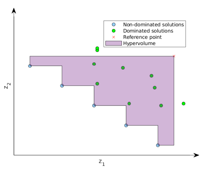
To evaluate the performance of a non-dominated solution set obtained by a multi-objective optimization algorithm there are several performance indicators in the literature that could be used. The hypervolume indicator (Zitzler & Thiele 1998) is very popular in the evolutionary multi-objective optimization community and will be used in this study. This indicator is also known as the Lebesgue measure and it is determined by quantifying the region in the objective space enclosed by the front of the non-dominated solutions and an upper-bounded reference point (assuming minimization). An illustration that shows the hypervolume for a hypothetical two-objective problem is depicted in Figure 2. Improving the hypervolume means increasing the area between the non-dominated solutions and the reference point, and this could be achieved by either improving the convergence (i.e., solutions with better performance with respect to both objectives) or improving the spread across the front (i.e., generating a higher density of more evenly spread non-dominated solutions). To compute the hypervolume value we use an exact dimension-sweep algorithm (Fonseca et al. 2006).
Overview of model discovery process
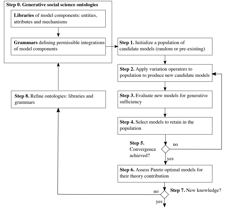
A schematic of the overall model discovery process is shown in Figure 3. Step 0 represents a pre-condition for the model discovery process. We define a library of theory building blocks implemented as model components and a grammar to guide the search process. Step 1 to 6 is the Grammatical Evolution process. In Step 1, an initialized population of models is generated. In Step 2, variation operators, e.g., crossover and mutation, are applied to produce new candidate models. In Step 3, the models in the current population are evaluated for generative sufficiency. Step 4 selects the models to retain in the population. If convergence is not achieved, go back to Step 2. If the convergence is achieved, the Pareto optimal model structures will be assessed for their theoretical contribution. Afterwards, if improvement is needed, the whole process can be restarted by adjusting the grammar or the library of components.
Grammar
In this study, our interest is to find model structures and parameters that offer the best trade-offs between the complexity of the model and the goodness-of-fit with respect to multiple targets. The model structure and the model parameters are separated in a bi-level formulation, where for each model structure identified by the GP algorithm at the upper-level, there is a separate calibration process being conducted to identify the best parameters at the lower-level. The goal is to find the model structure and parameters that will provide the best goodness-of-fit. This is known as a nested approach in the bi-level optimization literature (Sinha et al. 2018), which is commonly used in conjunction with evolutionary computation algorithms, such as genetic algorithms, differential evolution, and swarm intelligence. We did not use advanced bi-level optimization but addressed the bi-level problem by building constants and allowing the model discovery process to select promising parameter sets and agent heterogeneity distributions from calibrated results. However, to our knowledge, this is the first time that this approach has been used in conjunction with a GE algorithm. The following paragraphs describe in detail how the grammar incorporates both model structures and parameters.
The grammar describes which components in agent behavioral rules will be considered and how they can be combined together. This study focuses on agents’ daily decisions of which drinking schema to perform. The structure of the agents’ intention pathway will be exposed to the model discovery process. The intention is a function that determines the probability of choosing a drinking schema based on the following components: desire to drink (i.e., attitude to drinking) and the social norm theory concepts (injunctive norms, descriptive norms and autonomy). Refer to Table 2 for further details of the components of the intentional pathway. For the individual-level components autonomy and automaticity (the latter determining the likelihood of the intention pathway being triggered), the grammar also defines options for specifying the distribution across agents.
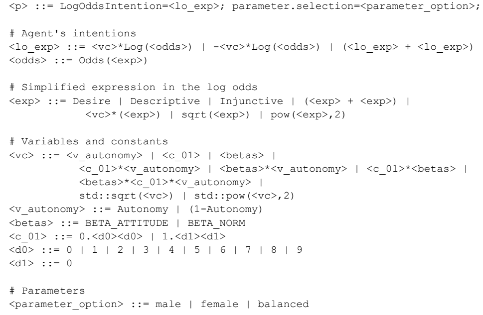
Figure 4 describes the grammar that guides the model discovery process. Each candidate (a program (<p>)) contains two expressions: one for the log odds intention and one for selecting a parameter set. Each expression can be formed only by a defined combination of expressions, variables, constants, and distribution options. This hierarchical grammar captures the complexity of different expressions.
The intention pathway uses a log odds function for each schema because, in the model, the probabilities of instantiating each drinking schema are represented using a multinomial logit equation. The log odds expression <lo_exp> can be modified by multiplying log odds with a variable/constant expression <vc> or -<vc>, or by summing two log odds.
The variable/constant expression <vc> can be constructed from a combination of agents’ autonomy (Autonomy, (1-Autonomy)), calibrated parameters for the agent intention (BETA_ATTITUDE, BETA_NORM), a constant between 0 and 1 (<c_01>), and the product of autonomy, a calibrated parameter and a constant. <vc> can also apply a square-root operator, or raise to the power of 2.
The expression within the odds <exp> can be constructed with normtheory concepts Desire, Descriptive, Injunctive and several operations (sum, multiplication, square root, raising to the power of 2). The odds expression is simplified in the grammar. In the implementation, the odds expression will be converted to expression of schema \(j\) over expression of schema \(0\). For example, if the expression is \(Desire+Injunctive\) then the full log odds function for schema \(j\) of agent \(i\) will be \(LogOddsIntention_i[j] = log((Desire_i[j]+Injunctive_i[j]) / (Desire_i[j=0]+Injunctive_i[j=0]))\).
Finally, for parameter selection, model parameters can be selected according to three calibrated parameter sets: <parameter_option>: male, female, or balanced. These options correspond to the three calibrated parameter sets that have the lowest implausibility when considering only male goodness-of-fit, considering only female goodness-of-fit, and balancing both simultaneously.
Experimental setup
The MOGGP algorithm is configured as follows. We defined a budget of 500 candidate model structures per population for up to 50 generations. We terminated the MOGGP early if convergence appeared to have been achieved according to the hypervolume metric. The GP variation operators are 75% subtree crossover and 25% subtree mutation. To account for model stochasticity, runs for each model structure are replicated 10 times with different random number seeds, with implausibilities computed as in Equations 3 and 4. It is computationally intensive to do a complete run of MOGGP, the process taking approximately 3 hours per generation on an i9-7980XE processor with 36 cores. We were unable to engage in hyperparameter tuning of the MOGGP configuration due to the run-time constraints, instead relying on default settings from the PonyGE2 toolbox. The source code to set up the MOGGP is available at: https://bitbucket.org/r01cascade/ge_norm_igss/
We use the annual time series data from 1985–2010 to compute implausibilities of the model structures during the MOGGP run. We reserve 2011–2015 data to validate the non-dominated structures that are identified during the structural calibration.
Results
Parameter calibration results for the original model structure
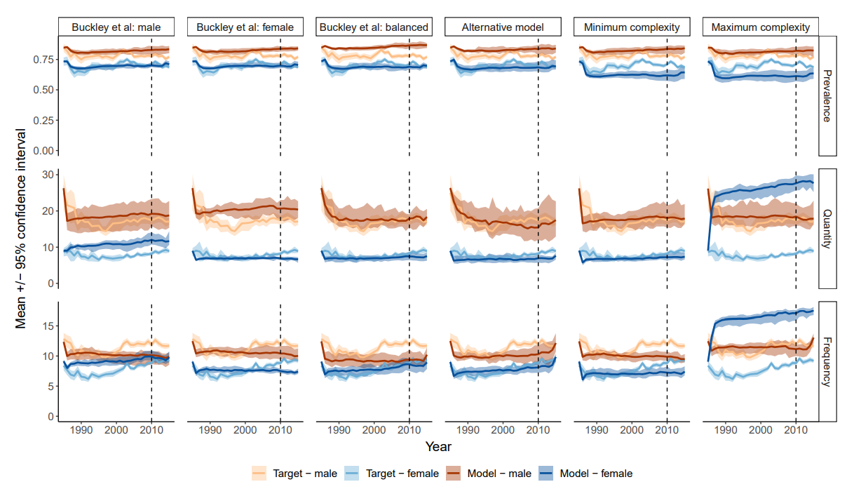
Parameter calibration was undertaken for the original model structure, both to identify how this structure would perform on targets for New York State and to provide parameter sets that could be used by the MOGGP. This calibration identified a trade-off between male and female implausibility, with parameter settings identified for: (a) lowest male implausibility; (b) lowest female implausibility; (c) a compromise between male and female implausibilities. The time series associated with each of these parameter sets is shown in the three left-hand columns in Figure 6. The top row of the figure shows the prevalence of drinking over time in the population split by male (red) and female (blue). The middle row shows the quantity of drinking over time (in grams of ethanol per day amongst drinkers). The bottom row shows frequency of drinking (average number of drinking days per month amongst drinkers). A clear trade-off between male and female performance can be seen. In particular, the model that is the best fit for males has a poor fit on female quantity and shows convergence of male and female frequency over time. Similarly, the model that is the best fit for females overestimates both prevalence and quantity for males. None of the calibrated models using the Buckley et al. (2022a) baseline structure are able to capture trends in male quantity towards the end of the calibration window.
The population-level weightings identified for attitudes and norms in the equation for agent intention are shown in Table 4, together with summaries of the individual heterogeneity for autonomy, automaticity and the history window for habits. These parameterizations are subsequently made available to the MOGGP process.
| Calibrated parameter values | |||
|---|---|---|---|
| Parameter | Lowest male implausibility | Lowest female implausibility | Balanced implausibility |
| Population-level | |||
| BETA_ATTITUDE | 0.976 | 0.967 | 0.918 |
| BETA_NORM | 0.664 | 0.818 | 0.868 |
| Individual-level | |||
| Mean Autonomy (SD) | 0.68 (0.37) | 0.86 (0.22) | 0.48 (0.39) |
| Mean automaticity (SD) | 0.22 (0.23) | 0.20 (0.15) | 0.32 (0.29) |
| Mean habit history window in days (SD) | 64 (32) | 89 (42) | 67 (33) |
Structural calibration results
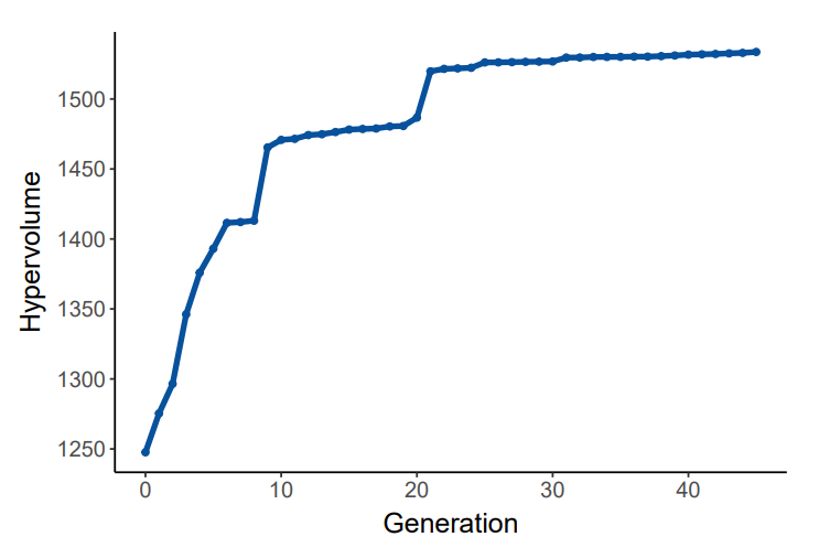
The hypervolume indicator was computed for each generation and monitored online during the MOGGP run. As shown in Figure 5, the indicator begins to saturate from generation 30 and we terminated the run at generation 45 when little further progress was being achieved.
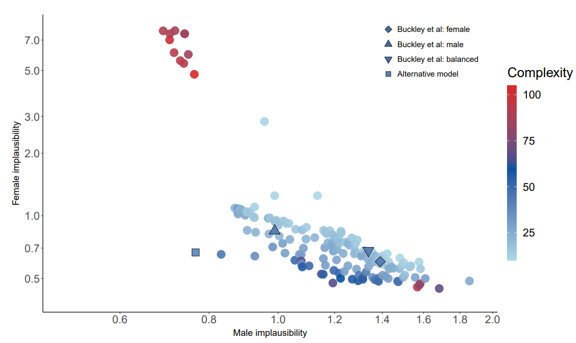
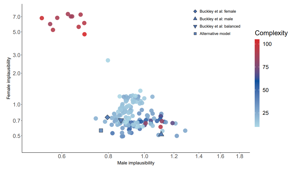
The Pareto front corresponding to the 157 non-dominated model structures contained in the final generation of the MOGGP population is shown in the scatterplot in Figure 7. The horizontal and vertical axes represent male and female implausibility respectively. The colour represents the complexity. Each point shown is a non-dominated model structure. The parameter calibration results for the original Buckley et al. (2022a) model are also superimposed on the scatterplot: lowest male implausibility (triangle shape), lowest female implausibility (diamond shape) and the compromise parameterization (inverted triangle shape). These comparator models are all of complexity 42. The square shaped point relates to a discovered ‘alternative’ model structure that is discussed in more detail below.
The Pareto front is convex and identifies several auto-generated model structures that dominate the parameter calibrations of the original model. The front is composed of two distinct regions. The first region, to the lower-right of the plot, consists of, for the most part, relatively low complexity structures that provide good female implausibility but relatively poor male implausibility. Within this region, there is a consistent trade-off between low complexity and higher, but still modest, complexity structures. There are also a few high complexity structures to the right of this region that provide very marginal gains in female implausibility for marginal losses in male implausibility. The second region, to the upper-left of the plot, consists of relatively high complexity structures that perform best in terms of male implausibility but worst in terms of female complexity, with marginal improvements in male implausibility being achieved at the expense of a large deterioration in female implausibility. It is possible that the Pareto front is disconnected between these two regions. There exists a solution of special interest in the space between these two regions (sometimes referred to as the ‘knee region’), which appears to offer a balanced trade-off between male and female implausibility without requiring a substantially complex structure. We investigate this alternative candidate structure (indicated by the square shape) further below.
Validation of identified model structures
The performance of the identified model structures on the validation window, 2011–2015, is shown in the scatterplot in Figure 8. Some bunching of the original lower-right region of the Pareto front is observed, with less of a trade-off between implausibility and complexity. This behavior is likely to be because the validation target time series has a smaller dynamic range than the calibration time series (as seen in Figure 6), allowing some of the low complexity structures that display flat dynamics to perform relatively well. High complexity structures from this region are now seen to perform relatively badly, indicative of over-fitting to the calibration data. While we might have suspected that the high complexity structures from the original upper-left region of the Pareto front would also see a similar deterioration in performance, this part of the front actually retains its position relative to the lower-right region. The candidate solution identified in the knee region of the calibration Pareto front is also located in the knee region of the validation front, but its relative advantage over other structures, in terms of implausibility, is reduced.
Discussion
Model discovery findings
Drinking behavior by gender
The original Buckley et al. (2022a) model exhibits issues in simultaneously reproducing both male and female drinking patterns over time. The parameter calibration was able to reproduce female quantity targets better than male, and particularly struggled to reproduce the increase in male drinking frequency observed after the year 2000 in all three parameterizations that were identified. The alternative model identified by the MOGGP leads to substantial improvements in model fit, retaining the good fit to the female targets and improving the fit to the male targets, and is able to reproduce the increase in male drinking frequency.
Theoretical interpretability and plausibility of the identified model structures
The complexity of the model structures varies between 10 (the simplest model) and 105 (the most complex model). For parameter selection, 17 structures use the male option, 134 use female, and five use balanced. We picked four structures for discussion: the original model structure from Buckley et al. (2022a), a structure with the simplest complexity, a structure with the highest complexity, and the alternative candidate structure which has an interpretable complexity and can achieve low implausibility for both male and female drinking trends. Structures picked for discussion are highlighted in Listing 1 alongside the three objective values: [male implausibility \(z_{1,\textrm{male}}\), female implausibility \(z_{1,\textrm{female}}\), complexity \(z_2\)].
LogOddsIntention=((BETA_ATTITUDE*Autonomy*Log(Odds(Desire)) +
                (BETA_NORM*0.50*(1-Autonomy)*Log(Odds(Descriptive)) +
BETA_NORM*0.50*(1-Autonomy)*Log(Odds(Injunctive))));LogOddsIntention=BETA_ATTITUDE*Log(Odds(Desire));
parameter.selection=male;LogOddsIntention=(((BETA_ATTITUDE*Autonomy*Log(Odds(Desire)) +
BETA_ATTITUDE*Autonomy*Log(Odds(Injunctive))) +
(-BETA_NORM*Autonomy*Log(Odds(Descriptive)) + -(1-Autonomy)*Log(Odds(Desire)))) +
((1.00*(1-Autonomy)*Log(Odds(sqrt(Desire))) +
BETA_NORM*(1-Autonomy)*Log(Odds(sqrt(sqrt(sqrt(pow(BETA_NORM,2)*(sqrt(((sqrt(Desire) +
sqrt(Desire)) + BETA_NORM*(pow(Descriptive,2))))))))))) +
(-BETA_NORM*Log(Odds((Descriptive + Desire))) + BETA_NORM*Log(Odds(Desire)))));
parameter.selection=male;LogOddsIntention=((BETA_ATTITUDE*Log(Odds(Injunctive)) +
-BETA_ATTITUDE*(1-Autonomy)*Log(Odds(BETA_NORM*(sqrt(Descriptive))))) +
BETA_NORM*Autonomy*Log(Odds(Desire)));
parameter.selection=balanced;For models with a complexity of less than 18, the structures only contain Desire, weighted by different constant parameters. For example, Listing 1b shows the simplest structure with complexity 10 and is the product of Desire and the population-level attitude weighting BETA_NORM. In the context of social norm theory, when the log odds intention consists of only Desire, the agents follow their past behavior initialized at baseline. This will produce a time series in which drinking prevalence, quantity, and frequency are relatively stable over time. Multipliers on Desire will act to scale the drinking level up or down. This effect can be seen in Figure 6, where the model with the lowest complexity exhibits an immediate drop in the time series to roughly the average of the target trend, followed by stability for the remainder of the time period.
The alternative perspective that the MOGGP identified contains all of the theoretical components from the original Buckley et al. (2022a) model—see Listing 1a and Listing 1d for a comparison of structures—but suggests an alternative mechanism for how these concepts are combined to derive intentions to drink. In this alternative perspective, all of the theoretical constructs from the original model, including both descriptive and injunctive norms, desire to drink and autonomy, were used to calculate intentions, suggesting that these are all of theoretical importance for determining individuals’ intentions to drink. In contrast to the original model, whereby the normative component was calculated as an equally weighted average of injunctive and descriptive norms, different constants are applied to injunctive and descriptive norms in the alternative model, suggesting that these may be weighted differently in the calculation of overall norms. This alternative formulation has some support in empirical research. In a study exploring the independent contribution of injunctive and descriptive norms for determining drinking intentions in US university students, Park et al. (2009) found that both types of norms were independent predictors of intention to drink, supporting our alternative model’s differential weighting of these constructs. This is further supported by a meta-analysis finding that descriptive norms had a slightly higher weighting on behaviors compared to injunctive norms (Rivis & Sheeran 2017).
Several components of the alternative model are not supported by the literature and warrant further investigation. First, the inverse of autonomy is used to determine how much individuals consider the descriptive norm when deciding their drinking, suggesting that individuals with lower autonomy rebel against the descriptive norm more than individuals with greater autonomy. This is the opposite of what we would expect; the concept of autonomy is intended to represent an individual’s susceptibility to normative influence and therefore more susceptible individuals would be expected to pay more attention to the norm. There is limited evidence on the individual-level factors influencing the distribution of autonomy in the population. However the candidate model goes against evidence suggesting that there are individual-level factors, including self-control (Robinson et al. 2015) and socio-demographic factors (Edwards et al. 2019) that bias individuals towards paying more or less attention to norms about drinking. Although more evidence is required on the factors influencing autonomy at the individual-level, it is possible that tying the distribution of autonomy to individual-level factors other than sex and alcohol consumption could improve model fit. A second component with limited empirical evidence is the negative contribution of descriptive norms to decisions to drink. This is incongruent with previous literature; meta-analyses consistently find that both injunctive and descriptive norms are positive predictors of behavior—i.e., the more ‘normal’ a behavior is, the more people will be motivated to act out that behavior (Rivis & Sheeran 2017). In summary, although the alternative model structure may usefully suggest a differential weighting on descriptive and injunctive norms, the original Buckley et al. (2022a) model remains more consistent overall with the wider empirical literature on normative behavioral influences on alcohol use.
Interpretability challenge
Models with high complexity are extremely difficult to interpret. For the structure with the highest complexity, all of the dynamic concepts from the Buckley et al. (2022a) model are used (see Listing 1c); however, this model is challenging to accept as theoretically meaningful. In the time series in Figure 6, the model produces trends in alcohol use behaviors that adequately fit targets for men, but struggle to fit female targets at all and vastly overestimates female drinking frequency and quantity, while underestimating prevalence.
Other strategies can be used during the model discovery process for improving theoretical interpretability, include simplifying the function before evaluation, limiting the tree depth in the GE configuration, or restricting the grammar. While designing the grammar, modelers have to be careful to balance exploration capability and interpretability. Since the model attempts to speak to theory and to policy logic models, it is important to leverage the model discovery process for theoretical interpretability and generative explanation.
To evaluate theoretical credibility, domain experts can be involved to assess the discovered structures (Step 6 of Figure 3). Tuong M. Vu et al. (2020) demonstrated the involvement of domain experts to interpret and evaluate the theoretical credibility of a role theory model. To consistently assess the credibility, three qualitative criteria were proposed: (1) at least one of the theory constructs must be implicated in the model dynamics; (2) the theory constructs must be used to represent mechanisms, rather than being proxies for black-box variable-centric explanation; (3) the model equations that describe the mechanisms must be compatible with the causal logic and evidence base for the theory. Since quantitative criteria may be difficult to develop for theoretical credibility assessment (beyond crude metrics of model complexity), identifying qualitative criteria like these is imperative for achieving consistency over judgments. In the case of the most promising MOGGP candidate structure, the model satisfies the first and second criteria, but its ability to satisfy the third criterion is called into question.
The evolution of structure
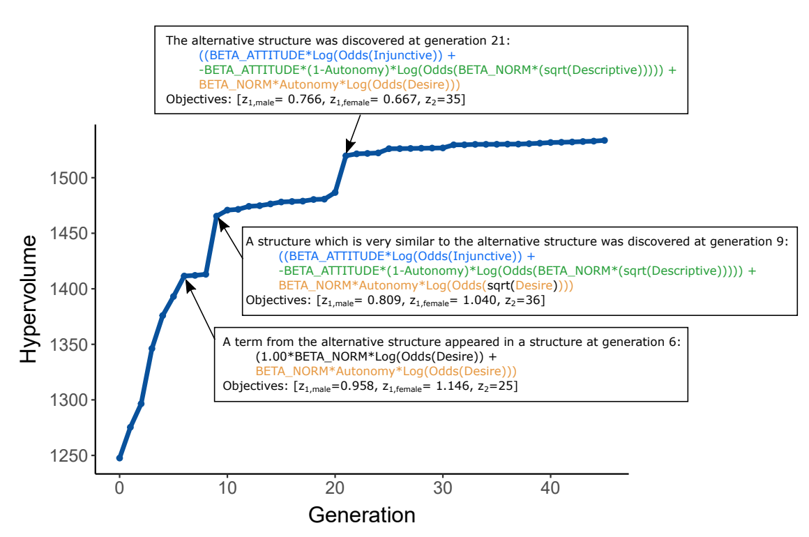
It is informative to consider the pathway the MOGGP took in evolving the candidate structure in Listing 1d. By looking through the history of the MOGGP populations, we have been able to identify structural ‘DNA’ for the candidate model and how these discoveries affected the convergence of the algorithm. As shown in Figure 9, the component term BETA_NORM*Autonomy*Log(Odds(Desire)) was first identified at generation 6 as part of a model that did not include normative elements. This model performed reasonably for males but less well for females (as a model that only amplifies Desire, it would produce relatively flat dynamics). At generation 9, a model emerged that was very similar to the final structure. This model contains injunctive and descriptive norms components, but the Desire term is now contained within a square-root operator, which will act as a nonlinear amplifier on agent attitudes. The inclusion of normative components enables the model to produce dynamics that improve the fit to both the male and female target trends, but at the cost of increased complexity. Despite only requiring a single change, the final model was not discovered until generation 21—here, the square-root operator is removed leading to substantial improvements in goodness-of-fit, particularly for female implausibility. Monitoring of the contributions that different candidate structures make to improving convergence may be useful in highlighting points in the model discovery process where the theory contributions of models could be assessed and changes to grammar made, if appropriate (see the discovery process schematic in Figure 3).
Limitations of iGSS as a method for mechanism identification
Alcohol use in New York State followed gentle trends over the study period, arguably indicative of a low-order dynamical system that is not prone to volatility. This period does not capture shocks that may activate the causal mechanisms that tend to cause instability or phase transitions (e.g., the pandemics of the early twentieth and twenty-first centuries, the impact of major human conflicts such as World War 2, or major interventions such as ‘Prohibition’—the 18th Amendment to the US Constitution that prohibited the manufacture, transportation and sale of alcohol in the US from 1920 to 1933). As such, the range of causal mechanisms that can be identified is limited and the findings cannot be confidently extrapolated outside of the specific spatio-temporal setting of New York State from the mid-1980s to mid-2010s. We cannot claim to have identified candidate mechanisms associated with Prohibition and so would not consider the model to have utility in predicting the effects of a new prohibition era. However, the ambitions of contemporary alcohol policymakers are typically more modest, being related to the scale of policies seen over the study window (e.g., changes in taxation and licensing laws).
Our findings do not allow conclusions to be drawn about the ability of iGSS to identify mechanisms driving dynamics in higher-order systems (e.g., systems which may exhibit phase transitions for small changes in system parameters or initial conditions). However, it is worth noting that existing model discovery works have demonstrated success in recovering cellular automata rules and network structures for chaotic systems (Yang & Billings 2000) and nonlinear differential equations for the classic Lorentz system (Ribera et al. 2022).
In principle, regardless of the order of the system, there could be a very large (potentially infinite) set of configurations of contingent mechanisms that could generate a given phenomenon. In earlier work, we have motivated iGSS by arguing explicitly for a plurality of mechanisms to be considered (Vu et al. 2020a). We believe that iGSS approaches should seek to promote diversity in the structures that are identified. More could be done in this area, by introducing explicitly diversity-promoting mechanisms—such as niching—as has been achieved for parameter estimation (Purshouse et al. 2014). Lawson (1997) has argued that the inability to differentiate between multiple candidate models using the existing data should not be regarded as a pathological ‘identification problem’, but rather indicates the need for further empirical investigation of the credible alternative explanations. We agree—iGSS should not be seen as a single isolated activity using frozen secondary datasets, but rather part of a reflexive and iterative process of scientific inquiry to better understand a phenomenon. Existing iGSS studies have tended to be presented as isolated computational activities focused on retrodiction of specific cases of a phenomenon, with work now needed to integrate the computational power of iGSS into broader retroductive frameworks incorporating a mix of quantitative and qualitative methods.
iGSS findings are contingent on the choice of targets. In our study, the targets we selected were population averages over time. While population average behavior is of key interest to alcohol harms prevention researchers (Skog 1985), we could instead have chosen metrics that captured the full distribution of behavior (e.g., Kolmogorov-Smironov statistics). Longitudinal surveys on alcohol use that are representative at state or country levels are not available for the US, so we could not use targets derived from individual trajectories of drinking. The choice of targets remains an open issue in iGSS but is likely to be application dependent. The iGSS process may have produced different findings if different targets had been available.
Conclusion
This paper has presented a novel computational social science method that uses multi-objective grammar-based genetic programming to explore different combinations of social theory concepts to search for alternative agent behavioral rules. The case study in alcohol use behaviors using concepts from social norm theory has been successful in showing how different arrangements of concepts from the theory produce different trade-offs between empirical goodness-of-fit and model interpretability. It would take human modelers an infeasible amount of time and effort to manually construct and explore the same number of realizations. These model discovery methods can be a tool to complement conventional model development and to help identify candidate mechanisms that better explain social phenomena.
The best calibrated parameterizations of the original Buckley et al. (2022a) model of social norms theory can partially explain male and female drinking trends in isolation. However no parameterisation was found which could explain both male and female drinking trends simultaneously, producing both male and female time series outputs with under one unit of implausibility. The MOGGP identified a candidate model that could meet this threshold for simultaneous goodness-of-fit, while also providing relatively good performance when validated. This model offers an interesting alternative perspective on how injunctive and descriptive norms come together with an agent’s autonomy to form an intention. However, the binding of autonomy with descriptive norms (i.e., that agents with less autonomy would act more strongly against descriptive norms) seems counter-intuitive. It is important to recognize that evidence to inform prior beliefs about the distribution of autonomy across the population was not available, with agent heterogeneity informed by the calibration process. As such, this apparently counter-intuitive finding may be an artefact of the model. It would be very beneficial for future social surveys to include instruments which estimate psychological attributes, to better inform iGSS efforts that leverage secondary data.
Joint structure-parameter calibration is a significant computational challenge for iGSS, since each candidate model structure requires its own parameter calibration. Previous approaches have either performed parameter calibration post-hoc (Vu et al. 2019) or provided a limited number of constants for the optimizer to choose from (Gunaratne & Garibay 2017a; Vu et al. 2020a). The present study provides a modest advance in this area—enabling the optimizer to build constants from components using the grammar and enabling it to choose from promising model parameter sets and distributions of agent heterogeneity. This type of approach is likely to be only locally optimal. Substantially more research is needed to provide a more robust solution to the joint structure-parameter problem, e.g., development of bi-level optimization approaches, including emulator technologies that can estimate the performance of a calibrated model structure without performing parameter calibration. The major challenge to emulation of model structure is the choice of an appropriate metric for measuring distances between candidate structures—Levenshtein distance is a possible contender but is, itself, computationally demanding to compute.
Our case study using social norm theory provided only a limited collection of theory building blocks for the iGSS process to work with. Further, we focused the study on the agent decision-making ‘rules’ (i.e., intentions) and did not consider changes to other mechanisms in the model (e.g., the perception of norms and processes that were modeled at the macro-level). The potential for iGSS as a cross-theory integration method remains largely unexplored, despite some fledgling work in this area integrating norm theory with role theory (Vu et al. 2021). There is presently a lack of available building blocks in the ABM community that are amenable to ‘plug-and-play’ iGSS, arguably due to the lack of uptake of any standard software engineering framework for specifying ABM models.
In our work, we have focused on empirical embeddedness as the key motivation for performing iGSS. However, iGSS may also have application beyond identifying candidate mechanisms that generate empirical phenomena. The method could also be used to identify mechanisms that could give rise to counterfactual or as yet unrealized dynamics, where the model discovery targets describe outcomes—possible futures—that are desirable (or otherwise) for society.
Acknowledgements
Research reported in this publication was supported by the National Institute on Alcohol Abuse and Alcoholism of the National Institutes of Health [Award Numbers R01 AA024443 and P50 AA005595] and Wave 1 of The UKRI Strategic Priorities Fund under the EPSRC Grant EP/W006022/1, particularly the “Shocks and Resilience” cross-theme within that grant & The Alan Turing Institute. This research was conducted as part of the Calibrated Agent Simulations for Combined Analysis of Drinking Etiologies (CASCADE) project and we would like to thank the whole CASCADE team for their input to wider discussions in generating the research reported in this paper. TMV designed and implemented the evolutionary process; AB, CB, JME and RCP contributed to overall model development and specification of the model discovery process, with model implementation by TMV; JAD generated results; RCP led the research; RCP, CB, TMV and JAD wrote the manuscript, which was reviewed by all authors. The authors have no conflicts of interest.
Notes
The schema are unordered since they are intended to represent qualitatively different drinking practices, rather than implying a latent preference for ethanol quantity.↩︎
We use random selection without replacement to avoid random drift in the agent’s habitual behavior over time.↩︎
This large number of attributes is a disadvantage of assuming unordered schema. If the schema were ordered, e.g., according to preference for ethanol quantity, then only three attributes would be necessary.↩︎
Other attributes, e.g., ethnicity, could also be used to define the reference group, which is conceptualized as a proxy for an agent’s identity.↩︎
Further details about the NAS series can be found in Kerr et al. (2009, 2013).↩︎
A computer program in this context could be an algorithm, a machine or even a brain.↩︎
References
AJZEN, I. (1991). The theory of planned behavior. Organizational Behavior and Human Decision Processes, 50(2), 179–211. [doi:10.1016/0749-5978(91)90020-t]
ATKINSON, J., Knowles, D., & Wiggers, J. (2018). Harnessing advances in computer simulation to inform policy and planning to reduce alcohol-related harms. International Journal of Public Health, 63, 537–546. [doi:10.1007/s00038-017-1041-y]
AXTELL, R. L., Epstein, J. M., Dean, J. S., Gumerman, G. J., Swedlund, A. C., Harburger, J., Chakravarty, S., Hammond, R., Parker, J., & Parker, M. (2002). Population growth and collapse in a multiagent model of the Kayenta Anasazi in Long House Valley. Proceedings of the National Academy of Sciences, 99(3), 7275–7279. [doi:10.1073/pnas.092080799]
BEVEN, K. (1993). Prophecy, reality and uncertainty in distributed hydrological modelling. Advances in Water Resources, 16(1), 41–51. [doi:10.1016/0309-1708(93)90028-e]
BOERO, R., & Squazzoni, F. (2005). Does empirical embeddedness matter? Methodological issues on agent-based models for analytical social science. Journal of Artificial Societies and Social Simulation, 8(4), 6.
BRENNAN, A., Buckley, C., Vu, T. M., Probst, C., Nielsen, A., Bai, H., Broomhead, T., Greenfield, T., Kerr, W., Meier, P. S., Rehm, J., Shuper, P., Strong, M., & Purshouse, R. C. (2020). Introducing CASCADEPOP: An open-source sociodemographic simulation platform for us health policy appraisal. International Journal of Microsimulation, 13(2), 21–60. [doi:10.34196/ijm.00217]
BUCKLEY, C., Brennan, A., Kerr, W., Probst, C., Puka, K., Purshouse, R., & Rehm, J. (2022a). Improved estimates for individual and population-level alcohol use in the United States, 1984-2020. International Journal of Alcohol and Drug Research, 10(1), 24–33. [doi:10.7895/ijadr.383]
BUCKLEY, C., Field, M., Vu, T. M., Brennan, A., Greenfield, T. K., Meier, P. S., Nielsen, A., Probst, C., Shuper, P. A., & Purshouse, R. C. (2022b). An integrated dual process simulation model of alcohol use behaviours in individuals, with application to US population-level consumption, 1984-2012. Addictive Behaviors, 124, 107094. [doi:10.1016/j.addbeh.2021.107094]
CASTILLO-CARNIGLIA, A., Pear, V. A., Tracy, M., Keyes, K. M., & Cerdá, M. (2019). Limiting alcohol outlet density to prevent alcohol use and violence: Estimating policy interventions through agent-based modeling. American Journal of Epidemiology, 188(4), 694–702. [doi:10.1093/aje/kwy289]
CENTERS for Disease Control and Prevention (CDC). (2019). Behavioral Risk Factor Surveillance System Survey Data. Available at: https://www.cdc.gov/brfss/data_documentation/index.htm
COLLIER, N., & North, M. (2013). Parallel agent-based simulation with Repast for High Performance Computing. SIMULATION, 89(10), 1215–1235. [doi:10.1177/0037549712462620]
COOKE, R., Dahdah, M., Norman, P., & French, D. P. (2016). How well does the theory of planned behaviour predict alcohol consumption? A systematic review and meta-analysis. Health Psychology Review, 10(2), 148–167. [doi:10.1080/17437199.2014.947547]
COTTINEAU, C., Reuillon, R., Chapron, P., Rey-Coyrehourcq, S., & Pumain, D. (2015). A modular modelling framework for hypotheses testing in the simulation of urbanisation. Systems, 3(4), 348–377. [doi:10.3390/systems3040348]
CRAIG, P., Dieppe, P., Macintyre, S., Michie, S., Nazareth, I., & Petticrew, M. (2008). Developing and evaluating complex interventions: The new Medical Research Council guidance. BMJ, 337. [doi:10.1136/bmj.a1655]
DEB, K., Pratap, A., Agarwal, S., & Meyarivan, T. (2002). A fast and elitist multiobjective genetic algorithm: NSGA-II. IEEE Transactions on Evolutionary Computation, 6(2), 182–197. [doi:10.1109/4235.996017]
EDWARDS, K. A., Witkiewitz, K., & Vowles, K. E. (2019). Demographic differences in perceived social norms of drug and alcohol use among Hispanic/Latinx and non-Hispanic White college students. Addictive Behaviors, 98, 106060. [doi:10.1016/j.addbeh.2019.106060]
EMMERICH, M. T. M., & Deutz, A. H. (2018). A tutorial on multiobjective optimization: Fundamentals and evolutionary methods. Natural Computing, 17, 585–609. [doi:10.1007/s11047-018-9685-y]
EPSTEIN, J. M. (1999). Agent-based computational models and generative social science. Complexity, 4(5), 41–60. [doi:10.1002/(sici)1099-0526(199905/06)4:5<41::aid-cplx9>3.0.co;2-f]
EPSTEIN, J. M. (2007). Generative Social Science. Princeton, NJ: Princeton University Press.
EPSTEIN, J. M. (2019). Inverse generative social science: What machine learning can do for agent-based modeling. In P. K. Davis, A. O’Mahony, & J. Pfautz (Eds.), Social-Behavioral Modeling for Complex Systems (pp. 779–780). Wiley. [doi:10.1002/9781119485001]
EPSTEIN, J. M. (2023). Inverse generative social science: Backward to the future. Journal of Artificial Societies and Social Simulation, 26(2), 9 [doi:10.18564/jasss.5083]
FENTON, M., McDermott, J., Fagan, D., Forstenlechner, S., Hemberg, E., & O’Neill, M. (2017). PonyGE2: Grammatical evolution in Python. Proceedings of the Genetic and Evolutionary Computation Conference Companion, New York, NY, USA [doi:10.1145/3067695.3082469]
FITZPATRICK, B. G., Martinez, J., Polidan, E., & Angelis, E. (2016). On the effectiveness of social norms intervention in college drinking: The roles of identity verification and peer influence. Alcoholism: Clinical and Experimental Research, 40(1), 141–151. [doi:10.1111/acer.12919]
FITZPATRICK, B., & Martinez, J. (2012). Agent-based modeling of ecological niche theory and assortative drinking. Journal of Artificial Societies and Social Simulation, 15(2), 4. [doi:10.18564/jasss.1926]
FITZPATRICK, B., Martinez, J., Polidan, E., & Angelis, E. (2015). The big impact of small groups on college drinking. Journal of Artificial Societies and Social Simulation, 18(3), 4. [doi:10.18564/jasss.2760]
FONSECA, C. M., Paquete, L., & López-Ibáñez, M. (2006). An improved dimension-sweep algorithm for the hypervolume indicator. Proceedings of the 2006 Congress on Evolutionary Computation (CEC’06) [doi:10.1109/cec.2006.1688440]
GARRISON, L. A., & Babcock, D. S. (2009). Alcohol consumption among college students: An agent-based computational simulation. Complexity, 14(6), 35–44. [doi:10.1002/cplx.20259]
GE, J., Polhill, J. G., Matthews, K. B., Miller, D. G., & Spencer, M. (2018). Not one Brexit: How local context and social processes influence policy analysis. PlOS One, 13(12), e0208451. [doi:10.1371/journal.pone.0208451]
GIABBANELLI, P., & Crutzen, R. (2013). An agent-based social network model of binge drinking among Dutch adults. Journal of Artificial Societies and Social Simulation, 16(2), 10. [doi:10.18564/jasss.2159]
GORMAN, D. M., Mezic, J., Mezic, I., & Gruenewald, P. J. (2006). Agent-based modeling of drinking behavior: A preliminary model and potential applications to theory and practice. American Journal of Public Health, 96(11), 2055–2060. [doi:10.2105/ajph.2005.063289]
GREENFIELD, T. K., & Room, R. (1997). Situational norms for drinking and drunkenness: Trends in the US adult population, 1979-1990. Addiction, 92, 33–47. [doi:10.1111/j.1360-0443.1997.tb03636.x]
GRIMM, V., Revilla, E., Berger, U., Jeltsch, F., Mooij, W. M., Railsback, S. F., Thulke, H.-H., Weiner, J., Wiegand, T., & DeAngelis, D. L. (2005). Pattern-oriented modeling of agent-based complex systems: Lessons from ecology. Science, 310(5750), 987–991. [doi:10.1126/science.1116681]
GRUENEWALD, P. J. (2007). The spatial ecology of alcohol problems: Niche theory and assortative drinking. Addiction, 102(6), 870–878. [doi:10.1111/j.1360-0443.2007.01856.x]
GUNARATNE, C., & Garibay, I. (2017a). Alternate Social Theory Discovery Using Genetic Programming: Towards Better Understanding the Artificial Anasazi. [doi:10.1145/3071178.3071332]
GUNARATNE, C., & Garibay, I. (2017b). Evolutionary model discovery of factors for farm selection by the Artificial Anasazi. Proceedings of the International Conference Computer Science and Engineering. [doi:10.1145/3145574.3145608]
GUNARATNE, C., & Garibay, I. (2020). Evolutionary model discovery of causal factors behind the socio-agricultural behavior of the Ancestral Pueblo. PLOS One, 15(12), e0239922. [doi:10.1371/journal.pone.0239922]
GUNARATNE, C., Rand, W., & Garibay, I. (2021). Inferring mechanisms of response prioritization on social media under information overload. Scientific Reports, 11(1). [doi:10.1038/s41598-020-79897-5]
HOLMES, J., Meier, P. S., Booth, A., Guo, Y., & Brennan, A. (2012). The temporal relationship between per capita alcohol consumption and harm: A systematic review of time lag specifications in aggregate time series analyses. Drug and Alcohol Dependence, 123(1–3), 7–14. [doi:10.1016/j.drugalcdep.2011.12.005]
IP, E. H., Wolfson, M., Easterling, D., Sutfin, E., Wagoner, K., Blocker, J., Egan, K., Rahmandad, H., & Chen, S. H. (2012). Agent-based modeling of college drinking behavior and mapping of system dynamics of alcohol reduction using both environmental and individual-based intervention strategies. Proceedings of the System Dynamics Conference
JACKSON, P., Reid, A., Huitson, N., Wuschke, K., & Dabbaghian, V. (2012). Drinking with friends: A cellular automata approach to modeling peer influence on binge drinking behavior. Proceedings of CAMUSS
KERR, W. C., Greenfield, T. K., Bond, J., Ye, Y., & Rehm, J. (2009). Age-period-cohort modelling of alcohol volume and heavy drinking days in the US National Alcohol Surveys: Divergence in younger and older adult trends. Addiction, 104(1), 27–37. [doi:10.1111/j.1360-0443.2008.02391.x]
KERR, W. C., Greenfield, T. K., Ye, Y., Bond, J., & Rehm, J. (2013). Are the 1976-1985 birth cohorts heavier drinkers? Age-period-cohort analyses of the National Alcohol Surveys 1979-2010. Addiction, 108(6), 1038–1048. [doi:10.1111/j.1360-0443.2012.04055.x]
KEYES, K. M., Schulenberg, J. E., O’Malley, P. M., Johnston, L. D., Bachman, J. G., Li, G., & Hasin, D. (2012). Birth cohort effects on adolescent alcohol use: The influence of social norms from 1976 to 2007. Archives of General Psychiatry, 69(12), 1304–1313. [doi:10.1001/archgenpsychiatry.2012.787]
KEYES, K. M., Shev, A., Tracy, M., & Cerdá, M. (2019). Assessing the impact of alcohol taxation on rates of violent victimization in a large urban area: An agent-based modeling approach. Addiction, 114(2), 236–247. [doi:10.1111/add.14470]
KOZA, J. R. (1992). Genetic Programming: On the Programming of Computers by Means of Natural Selection. Cambridge, MA: MIT Press.
LALLY, P., van Jaarsveld, C. H., Potts, H. W., & Wardle, J. (2010). How are habits formed: Modelling habit formation in the real world. European Journal of Social Psychology, 40(6), 998–1009. [doi:10.1002/ejsp.674]
LAMY, F., Perez, P., Ritter, A., & Livingston, M. (2011). SimARC: An ontology-driven behavioural model of alcohol abuse. SIMUL 2011: The Third International Conference on Advances in System Simulation
LAWSON, T. (1997). Economics and Reality. London: Routledge.
MANSON, S., Schroeder, J., van Riper, D., & Ruggles, S. (2019). IPUMS national historical geographic information system: Version 14.0 [dataset]. Available at: https://www.nhgis.org/revision-history
MCGILL, E., Petticrew, M., Marks, D., McGrath, M., Rinaldi, C., & Egan, M. (2021). Applying a complex systems perspective to alcohol consumption and the prevention of alcohol-related harms in the 21st century: A scoping review. Addiction, 116(9), 2260–2288. [doi:10.1111/add.15341]
O’NEILL, M., & Ryan, C. (2001). Grammatical evolution. IEEE Transactions on Evolutionary Computation, 5(4), 349–358.
O’NEILL, M., & Ryan, C. (2003). Grammatical Evolution: Evolutionary Automatic Programming in an Arbitrary Language. Springer.
OPENSHAW, S. (1983). From data crunching to model crunching: The dawn of a new era. Environment and Planning A, 15, 1011–1013.
PARK, H. S., Klein, K. A., Smith, S., & Martell, D. (2009). Separating subjective norms, university descriptive and injunctive norms, and U.S. descriptive and injunctive norms for drinking behavior intentions. Health Communication, 24(8), 746–751. [doi:10.1080/10410230903265912]
PEREZ, P., Dray, A., Moore, D., Dietze, P., Bammer, G., Jenkinson, R., Siokou, C., Green, R., Hudson, S. L., & Maher, L. (2012). SimAmph: An agent-based simulation model for exploring the use of psychostimulants and related harm amongst young Australians. International Journal of Drug Policy, 23(1), 62–71. [doi:10.1016/j.drugpo.2011.05.017]
PROBST, C., Vu, T. M., Epstein, J. M., Nielsen, A. E., Buckley, C., Brennan, A., Rehm, J., & Purshouse, R. C. (2020). The normative underpinnings of population-level alcohol use: An individual-level simulation model. Health Education & Behavior, 47(2), 224–234. [doi:10.1177/1090198119880545]
PURSHOUSE, R. C., Ally, A. K., Brennan, A., Moyo, D., & Norman, P. (2014). Evolutionary parameter estimation for a Theory of Planned Behaviour microsimulation of alcohol consumption dynamics in an English birth cohort 2003 to 2010 [doi:10.1145/2576768.2598239]
PURSHOUSE, R. C., Buckley, C., Brennan, A., & Holmes, J. (2021). Commentary on Robinson et al. (2021): Evaluating theories of change for public health policies using computer model discovery methods. Addiction, 116(10), 2709–2711. [doi:10.1111/add.15595]
REDFERN, J., Sidorov, K., Rosin, P. L., Moore, S. C., Corcoran, P., & Marshall, D. (2017). An open-data, agent-based model of alcohol related crime. 2017 14th IEEE International Conference on Advanced Video and Signal Based Surveillance (AVSS) [doi:10.1109/avss.2017.8078513]
RIBERA, H., Shirman, S., Nguyen, A. V., & Mangan, N. M. (2022). Model selection of chaotic systems from data with hidden variables using sparse data assimilation. Chaos, 32(063101). [doi:10.1063/5.0066066]
RICHARDS, F. C., Meyer, T. P., & Packard, N. H. (1990). Extracting cellular automaton rules directly from experimental data. Physica D, 45, 189–202. [doi:10.1016/0167-2789(90)90182-o]
RIVIS, A., & Sheeran, P. (2017). Descriptive norms as an additional predictor in the theory of planned behavior: A meta-analysis. Planned Behavior, 22, 218–233. [doi:10.4324/9781315126449-4]
ROBINSON, E., Jones, A., Christiansen, P., & Field, M. (2015). Drinking like everyone else: Trait self-control moderates the association between peer and personal heavy episodic drinking. Substance Use & Misuse, 50(5), 590–597. [doi:10.3109/10826084.2014.991407]
RODRÍGUEZ-VÁZQUEZ, K., Fonseca, C. M., & Fleming, P. J. (2004). Identifying the structure of nonlinear dynamic systems using multiobjective genetic programming. IEEE Transactions on Systems, Man, and Cybernetics Part A: Systems and Humans, 34(4), 531–545.
ROERECKE, M., & Rehm, J. (2010). Irregular heavy drinking occasions and risk of ischemic heart disease: A systematic review and meta-analysis. American Journal of Epidemiology, 171(6), 633–644. [doi:10.1093/aje/kwp451]
RUGGLES, S., Flood, S., Goeken, R., Grover, J., Meyer, E., Pacas, J., & Sobek, M. (2020). IPUMS USA: Version 10.0 [dataset]. Available at: https://www.ipums.org/projects/ipums-usa/d010.v10.0 [doi:10.1007/978-3-030-22009-9_980]
SCHMIDT, M., & Lipson, H. (2009). Distilling free-form natural laws from experimental data. Science, 324(5923), 81–85. [doi:10.1126/science.1165893]
SCHUHMACHER, N., Ballato, L., & van Geert, P. (2014). Using an agent-based model to simulate the development of risk behaviors during adolescence. Journal of Artificial Societies and Social Simulation, 17(3), 1. [doi:10.18564/jasss.2485]
SCOTT, N., Hart, A., Wilson, J., Livingston, M., Moore, D., & Dietze, P. (2016a). The effects of extended public transport operating hours and venue lockout policies on drinking-related harms in Melbourne, Australia: Results from SimDrink, an agent-based simulation model. International Journal of Drug Policy, 32, 44–49. [doi:10.1016/j.drugpo.2016.02.016]
SCOTT, N., Livingston, M., Hart, A., Wilson, J., Moore, D., & Dietze, P. (2016b). SimDrink: An agent-based NetLogo model of young, heavy drinkers for conducting alcohol policy experiments. Journal of Artificial Societies and Social Simulation, 19(1), 10. [doi:10.18564/jasss.2943]
SCOTT, N., Livingston, M., Reporter, I., & Dietze, P. (2017). Using simulation modelling to examine the impact of venue lockout and last-drink policies on drinking-related harms and costs to licensees. Australian and New Zealand Journal of Public Health, 41(3), 243–247. [doi:10.1111/1753-6405.12640]
SINHA, A., Malo, P., & Deb, K. (2018). A review on bilevel optimization: From classical to evolutionary approaches and applications. IEEE Transactions on Evolutionary Computation, 22(2), 276–295. [doi:10.1109/tevc.2017.2712906]
SKOG, O.-J. (1985). The collectivity of drinking cultures: A theory of the distribution of alcohol consumption. British Journal of Addiction, 80, 83–99. [doi:10.1111/j.1360-0443.1985.tb05294.x]
SMITH, V. A. (2008). Evolving an agent-based model to probe behavioral rules in flocks of cowbirds. Available at: https://vannesmithlab.wp.st-andrews.ac.uk/files/2015/08/Smith_ALifeXI08_Correction.pdf
SPICER, V., Reid, A. A., Ginther, J., Seifi, H., & Dabbaghian, V. (2012). Bars on blocks: A cellular automata model of crime and liquor licensed establishment density. Computers, Environment and Urban Systems, 36(5), 412–422. [doi:10.1016/j.compenvurbsys.2012.02.004]
STANKOV, I., Yang, Y., Langellier, B. A., Purtle, J., Nelson, K. L., & Diez Roux, A. V. (2019). Depression and alcohol misuse among older adults: Exploring mechanisms and policy impacts using agent-based modelling. Social Psychiatry and Psychiatric Epidemiology, 54, 1243–1253. [doi:10.1007/s00127-019-01701-1]
STEWART, E., & Smith, K. E. (2015). “Black magic” and “gold dust”: The epistemic and political uses of evidence tools in public health policy making. Evidence & Policy, 11(3), 415–437. [doi:10.1332/174426415x14381786400158]
THIELE, J. C., Kurth, W., & Grimm, V. (2014). Facilitating parameter estimation and sensitivity analysis of agent-based models: A cookbook using NetLogo and ’R’. Journal of Artificial Societies and Social Simulation, 17(3), 11. [doi:10.18564/jasss.2503]
VERNON, I., Goldstein, M., & Bower, R. G. (2010). Galaxy formation: A Bayesian uncertainty analysis. Bayesian Analysis, 5(4), 619–670. [doi:10.1214/10-ba524]
VU, T. M., Buckley, C., Bai, H., Nielsen, A., Probst, C., Brennan, A., Shuper, P., Strong, M., & Purshouse, R. C. (2020a). Multiobjective genetic programming can improve the explanatory capabilities of mechanism-based models of social systems. Complexity, 2020, 8923197. [doi:10.1155/2020/8923197]
VU, T. M., Davies, E., Buckley, C., Brennan, A., & Purshouse, R. C. (2021). Using multi-objective grammar-based genetic programming to integrate multiple social theories in agent-based modeling. In H. Ishibuchi, Q. Zhang, R. Cheng, K. Li, H. Li, H. Wang, & A. Zhou (Eds.), Evolutionary Multi-Criterion Optimization: EMO 2021 Proceedings (pp. 721–733). Springer. [doi:10.1007/978-3-030-72062-9_57]
VU, T. M., Probst, C., Epstein, J. M., Brennan, A., Strong, M., & Purshouse, R. C. (2019). Toward inverse generative social science using multi-objective genetic programming. Proceedings of the Genetic and Evolutionary Computation Conference, New York, NY, USA [doi:10.1145/3321707.3321840]
VU, T. M., Probst, C., Nielsen, A., Bai, H., Buckley, C., Meier, P. S., Strong, M., Brennan, A., & Purshouse, R. C. (2020b). A software architecture for mechanism-based social systems modelling in agent-based simulation models. Journal of Artificial Societies and Social Simulation, 23(3), 1. [doi:10.18564/jasss.4282]
WORLD Health Organization. (2018). Global status report on alcohol and health 2018. Geneva, ISBN: 978-92-4- 156563-9
YANG, Y., & Billings, S. A. (2000). Extracting Boolean rules from CA patterns. IEEE Transactions on Systems, Man, and Cybernetics - Part B: Cybernetics, 30(4), 573–581. [doi:10.1109/3477.865174]
ZHONG, J., Luo, L., Cai, W., & Lees, M. (2014). Automatic rule identification for agent-based crowd models through gene expression programming. Proceedings of the 2014 international conference on Autonomous Agents and Multi-Agent Systems [doi:10.1109/wsc.2014.7019906]
ZITZLER, E., & Thiele, L. (1998). Multiobjective optimization using evolutionary algorithms - A comparative case study. Parallel Problem Solving from Nature - PPSN V [doi:10.1007/bfb0056872]