The Role of Argument Strength and Informational Biases in Polarization and Bi-Polarization Effects

and
aCNR, Italy; bInstitute for Computational Linguistics «A. Zampolli», Italy
Journal of Artificial
Societies and Social Simulation 26 (2) 5
<https://www.jasss.org/26/2/5.html>
DOI: 10.18564/jasss.5062
Received: 20-Dec-2022 Accepted: 09-Mar-2023 Published: 31-Mar-2023
Abstract
This work explores, on a simulative basis, the informational causes of polarization and bi-polarization of opinions in groups. Here, the term `polarization' refers to a uniform change of the opinion of the whole group towards the same direction, whereas `bi-polarization' indicates a split of two subgroups towards opposite directions. For the purposes of the present inquiry we expand the model of the Argument Communication Theory of Bi-polarization. The latter is an argument-based multi-agent model of opinion dynamics inspired by Persuasive Argument Theory. The original model can account for polarization as an outcome of pure informational influence, and reproduces bi-polarization effects by postulating an additional mechanism of homophilous selection of communication partners. The expanded model adds two dimensions: argument strength and more sophisticated protocols of informational influence (argument communication and opinion update). Adding the first dimension allows to investigate whether and how the presence of stronger or weaker arguments in the discussion influences polarization and bi-polarization dynamics, as suggested by the original framework of Persuasive Arguments Theory. The second feature allows to test whether other mechanisms related to confirmation bias and epistemic vigilance can act as a driving force of bi-polarization. Regarding the first issue, the simulations we perform show that argument strength has a measurable effect. With regard to the second, our results witness that, in absence of homophily, only very strong types of informational bias can lead to bi-polarization.Introduction
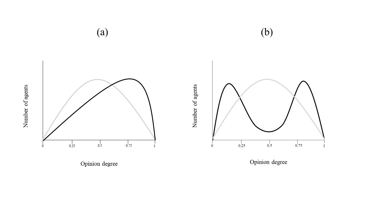
In the context of social psychology, group polarization indicates the well-documented phenomenon by which opinions of group members tend to shift in the same direction after discussion (Moscovici & Zavalloni 1969; Stoner 1961). This means that all individuals become more convinced of a given issue, or more inclined towards a given decision, than they were at the outset. Figure 1(a) represents a typical instance of this type of opinion dynamic. Here, at the beginning of the discussion (grey line), the degree of opinion of group members (relative to a specific issue) is almost normally distributed around the middle, in a scale from 0 (fully against) to 1 (fully pro), and then moves towards a pro- attitude at the end (black line). In the most current use of the word however, ‘polarization’ is employed to refer, although not univocally (Bramson et al. 2017), to a bimodal distribution of opinions, i.e., to the formation of two cohesive clusters of people at opposite poles of a spectrum. Group polarization, as introduced here, is something different, being rather a particular form of group consensus, where all individuals align in a specific manner. Bimodal distribution is nonetheless most likely to emerge as a by-product of two distinct dynamics of group polarization that lead the two sub-groups’ opinions in opposite directions (Figure 1(b)). Here, we follow Mäs & Flache (2013) and refer to such dynamics as bi-polarization effects, or simply as bi-polarization. Seen from this angle, polarization is a necessary although not a sufficient cause of bi-polarization. It should be noted that after fleshing out the mechanisms that generate polarization, the reasons that determine a split towards opposite directions may still remain obscure.
From a normative perspective, one big question is whether polarization and bi-polarization can occur in a group of rational agents, or rather if some irrational bias is a necessary ingredient for their emergence. Some recent formal approaches to the question supposedly show that even bi-polarization may be due to purely rational causes related to how agents update their opinion in the light of new information. We discuss two of them later on in Section 5 (Jern et al. 2014; Singer et al. 2019). As we shall see, they build upon different rationality frameworks and what is more, on many additional modelling assumptions whose consequences are difficult to assess. Here, we prefer not to provide a fully-fledged definition of rational behaviour and avoid approaching our question along these lines. Even if we abstain from defining the precise meaning of ‘rationality’ or ‘rational agent’, our previous considerations would suggest that, although the two phenomena are closely related, it may well be the case that group polarization does not require controversial mechanisms to arise – e.g., strong social or psychological biases on the agents’ side – while bi-polarization does. For these reasons, it is an interesting task to first isolate plausible minimal causes of group polarization and then see which additional triggering factors are needed to obtain bi-polarization effects. These are typical questions a simulative approach via artificial societies allows to address. Such additional factors may or may not fulfil a series of intuitive desiderata for rationality or for other epistemic virtues. Although we will suggest that some of them do, we do not take a strong stand on this matter.
Agent-based models (ABM) of opinion dynamics have been widely exploited to reproduce and understand these phenomena. Many of them come from the family of bounded confidence models (Deffuant et al. 2000; Hegselmann et al. 2002). Based on a different inspiration, we find argument-based ABMs (Banisch & Olbrich 2021; Mäs & Flache 2013; Taillandier et al. 2021). In particular, the model of the Argument Communication Theory of Bi-polarization (ACTB) by Mäs & Flache (2013) fulfils most desiderata for a minimal explanation, since polarization occurs as a natural outcome and bi-polarization emerges by simply postulating a moderate degree of homophily, which is the tendency of individuals to communicate more with those who share similar opinions. This model is inspired by Persuasive Arguments Theory (PAT) (Vinokur 1971; Vinokur & Burstein 1974), which assumes that opinion dynamics are influenced by the circulation of novel and persuasive arguments, and therefore are determined by informational influence. The ACTB model is a powerful proof of concept of PAT and serves as a main tool and a starting point of the present work. However, there are two relevant issues it does not allow to explore in its present form. The first one is instantiated by the following question:
- Question 1. Assume that, although equal in number, arguments favouring one side are objectively stronger, alias more persuasive, than arguments for the other side. Will this force general consensus towards the stronger side? And if not, will this at least push more individuals towards it?
This question is motivated by the fact that many real-life debates have a substantial imbalance between parties due to the bi-polarization process. One may think for example, about the recent debate over SARS-CoV-2 vaccines, where one party, although much more vocal, ends up being a clear minority in society (Lazarus et al. 2023). While PAT assumes that persuasiveness is a relevant dimension, in the original ACTB model all arguments have equal strength. As a result, it predicts that with an equal number of pro and con arguments, the average consensus will be mostly in the middle of the opinion scale, whereas when instead bipolarization occurs, the cardinality of the groups on the two sides of the opinion scale will be the same. With arguments of different strength, we can test whether the ‘stronger’ side has an advantage. A second issue is the following:
- Question 2. Can bi-polarization occur without homophily, as an effect of purely informational biases?
As mentioned previously, homophily is the unique possible trigger of bipolarization in the ACTB model. However, a long tradition in social and cognitive psychology identifies, as the main causes of polarization and bi-polarization, a number of informational biases somehow related to epistemic vigilance (Section 2). The protocol of informational influence of the original ACTB model – the way agents communicate and accept arguments for opinion update – ‘neutralizes’ the effect of such biases. In this respect, we can reproduce and operationalize them in the model, in order to test whether and how they can work as alternative minimal explanations.
The paper is organised as follows: In Section 2, we provide some general background on studies in social and cognitive psychology and how they inspire computational approaches. We specify general desiderata to answer questions 1 and 2. In Section 3 we introduce the formal tools for our work. First, we recap the general architecture of the ACTB simulation environment upon which we build, with focus on its informational influence phase and its measure of opinion strength. We then introduce our modifications to the ACTB environment. Here, we provide an alternative way of structuring argument-based information by means of quantitative bipolar graphs (Baroni et al. 2019) and consequently a new measure of opinion strength that generalizes the old one. Secondly, we intervene on the informational influence phase between agents, mostly on the mechanism of argument reception and opinion update by the receiver, so to encode different shades of information bias happening during communication. In Section 4, we illustrate the simulative setup that is meant to answer our two questions and show the results of our simulations. Finally, in Section 5 we discuss the general assumptions of the model in the context of these results and, as a consequence, their importance. We do this with special attention to the comparison with two alternative accounts of bi-polarization via informational influence. The first one is a family of Bayesian approaches (Angere 2010; Jern et al. 2014; Pallavicini et al. 2021). While our experiments show that in the absence of homophily, bi-polarization occurs only under very strong forms of bias, Bayesian models seem to predict the opposite. The second is an argument-based model of opinion dynamics Singer et al. (2019), very similar in spirit to the ACTB model.1 Here, the authors test the bipolarizing effect of three different opinion update policies which are, to different extents, similar to some of those we implement to answer Question 2. Under many respects, our results converge with theirs but, as we show, this is not the case when we introduce (even minimal) noise. This is the reason why our conclusions about the possibility of obtaining bi-polarization effects without bias are less ‘optimistic’.
Overview of the Problem and Desiderata for a Computational Model
Background in social and cognitive psychology
Explanations of how group polarization can emerge in a group fall into two big families, which can be labelled respectively as social influence and informational influence explanations. Briefly sketched, social influence explanations postulate the existence of a tendency of individuals to align their opinion with that held by other members of their group (and even a bit more extreme). This may be the effect of triggers such as social comparison (Sanders & Baron 1977) or self-categorization (Hogg et al. 1990). On the other side, informational influence explanations assume that these dynamics are caused by simply sharing information between participants and how they communicate evidence and update their opinion, regardless of who is talking to whom. In particular, PAT hypothesizes that, “group discussion will cause an individual to shift in a given direction to the extent that the discussion exposes that individual to persuasive arguments favouring that direction” (Isenberg 1986). Both explanations can account for the type of snowballing effect represented in Figure 1(a) and their assumptions have proven, in lab experiments, to be effective in different contexts (Isenberg 1986).
From our point of view, PAT has the advantage of explaining polarization without resorting to any kind of individual bias and in the context of fully open and trusted exchange of information among agents. Indeed, in typical lab experiments assessing how argument exchange induces polarization, every participant is equally likely to interact with any other and the experimental conditions (e.g., strong anonymity and trust of the interaction partner) guarantee by design that other factors are neutralized (Vinokur & Burstein 1974). Furthermore, the specific process by which PAT explains (argument-induced) opinion change helps dissolving the apparent weirdness of polarization dynamics, due to the unwarranted assumption that the opinions of any two individuals should come closer after they share information. Intuitively, if we take two agents with strong but different arguments supporting a given decision \(v\), mutual communication of such arguments will provide new reasons in favour of \(v\) to both agents, and therefore reinforce their positive attitude towards the decision. The same mechanism may of course work in the opposite direction.
Bi-polarization effects seem on the other hand somewhat harder to explain, within the context of PAT, without recurring to additional biases. On the contrary, experimental evidence seems to show that open interaction in diverse groups works against bi-polarization (Vinokur & Burnstein 1978). Usual suspects are then social influence biases, as self-categorization, that would push individuals to align their opinions with in-group members while distancing from out-group members. This mechanism of positive and negative influence is shown to work towards bi-polarization in bounded confidence models (Flache & Macy 2011). However, there is no clear experimental evidence that negative influence is effective in real-life scenarios (Berger & Heath 2008; Krizan & Baron 2007). In this respect we should ask ask whether informational biases play any role.
The recent interest raised in cognitive sciences by the argumentative theory of reasoning (Mercier & Sperber 2011, 2017) is a further reason why the study of informational influence via argument exchange is relevant. The latter assumes that all human reasoning is a cognitive module, which ‘evolved for the production and evaluation of arguments in communication’ (Mercier & Sperber 2011 p. 58) rather than, e.g., to perform strict logical inferences. From the point of view of this theory, many opinion dynamics, including polarization, should be regarded as natural by-products of how arguments are exchanged and processed by individuals in the social context of communication. Even detrimental phenomena related to polarization, such as groupthink (Janis 1983), are seen as natural side-effects, occurring when reasoning is used outside its natural context. This suggests that the crux of the matter may be how arguments are communicated and evaluated by individuals, and therefore that we also need to look into other informational biases, well-known to psychologists, as possible candidate causes of bi-polarization.
In the field of ABM research, bounded confidence models as Deffuant et al. (2000) or Hegselmann et al. (2002) hinge mostly within the realm of social influence. Internal factors that determine the degree of opinion of one agent are left as a black box. The degree of agents’ opinion is adjusted either by a mechanism of averaging2, when they meet agents with a sufficiently similar opinion (in-group members), or of distancing when they instead meet agents with a dissimilar opinion (out-group members).
As already mentioned, ACTB is the first computational approach inspired by PAT. Here, the agents’ opinion is determined as a function of their pro arguments weighted against their con arguments, and interaction consists of an exchange of arguments and then consequent opinion update. As we have said, ACTB does not account for the dimension of argument strength and therefore cannot address Question 1. Furthermore, it postulates homophily to obtain bi-polarization. Here, homophily has the effect of fostering opinion divergence, by making individuals with distant opinions less and less likely to share arguments and therefore determining the emergence of separate clusters, where individuals are likely to hear arguments confirming their acquired opinion. Arguably, if not social influence in disguise3, this can still be regarded as a bold assumption to make, since it prevents the discussion to be fully open among individuals. Homophily is absent in many of our experiments with the revised ACTB model. When this is the case, we can assume that we are in a pure informational scenario. This is understood as a situation where the outcome is determined solely by (a) the way agents communicate arguments and (b) how they revise their opinion on the basis of the new argument plus those which they already have and nothing else.
Introducing argument strength
Concerning argument strength, the use of the notion of an argument in the context of PAT should give us pause to think. First, arguments about some issue \(v\) are treated as generic items that may be weighted in favour or against \(v\). Further, even the strongest arguments are not treated as knockout reasons that could settle a given issue (such as, e.g., logically valid arguments), but rather as defeasible reasons for it. The justification they provide for \(v\) comes in degrees and displays a certain type of monotonic behaviour. By this we mean that, ceteris paribus, more arguments in favour of \(v\) will determine a more positive attitude towards \(v\) and viceversa. All these aspects are incorporated within the ACTB model.
As mentioned previously, unlike PAT, all arguments have equal weight in the ACTB approach vis-à-vis the debated issue. The implicit assumption here is that arguments are independent from one another. This is a useful simplification for the actual purposes of Mäs & Flache (2013), but overlooks a fundamental aspect of argumentation, i.e., that most of the times arguments bear articulated relationships on each other. For example, some arguments are counter-arguments to others supporting any given issue (e.g., by undermining their premises), or counter-counterarguments to them, or else supporters of counterarguments, and so on. In turn, these complex relationships affect the impact of each argument on the issue at stake.
To make this more intuitive, the two graphs in Figure 2 represent two possible ways an agent could be aware of two arguments supporting \(v\) (the topic node) and two arguments against \(v\) (more details in Section 3). Here, arguments are represented as nodes, while directed edges labelled with \(+\) indicate support, while those labelled with \(-\) indicate an attack against it. In the first graph, pro arguments \(a_1\) and \(a_2\) are not attacked, while in the second case they are (by counterargument \(b_1\)). At an intuitive level, one such argument, says \(a_1\), should have a different weight on \(v\) in different situations and therefore should affect the calculation of the strength of \(v\) in a different way (and this will be the case for the measures we define later). The fact that argumentation has a complex structure is not something that PAT explicitly takes into account. However, our approach accounts for its key dimension of persuasiveness and does this in a principled manner.
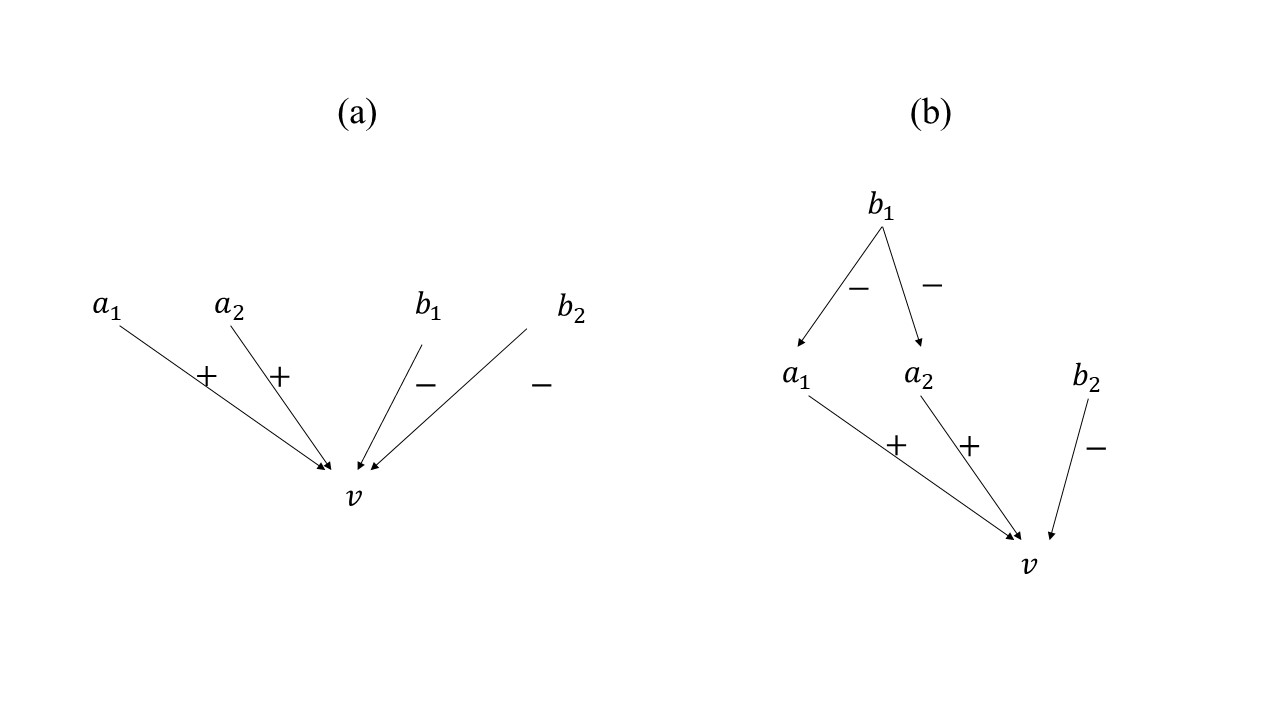
The graphs represented in Figure 2 are known in the field of formal argumentation as bipolar graphs (Cayrol & Lagasquie-Schiex 2009). If we endow a bipolar graph with a measure of argument strength, we get a quantitative bipolar graph (Amgoud & Ben-Naim 2016; Baroni et al. 2019; Cayrol & Lagasquie-Schiex 2005). This provides a useful formal tool to frame the knowledge of individuals concerning \(v\). The main idea and the first operational task here is to use these graphs in the ACTB model to represent the argumentative knowledge base of individuals and its transformation during an information exchange, i.e. discussion with others. In general, when an agent receives a new argument about a given topic, this enters a complex web of other arguments that constitute their knowledge base of \(v\) and altogether inform their opinion about it. The topology of this web of arguments is likely to influence the weight of the received argument as well as its acceptance by the agent.
Informational biases
The second main challenge for a simulative approach to PAT is to account for other strategies of argument communication and mechanisms of opinion update that may generate bi-polarization. In the original model of ACTB, when two agents are paired for an exchange at time \(t\), this occurs by speakers randomly communicating one argument they own, and by receivers automatically accepting it as its most recent piece of information, while discarding an older argument. On the one hand, the speakers select any argument, including those against their own opinion. On the other hand, the receivers accept the argument at face value. Arguably, this is not how human communication runs in most situations. Usually, speakers communicate arguments they take as more relevant, more informative or fit to their interests more. On the other side too, information is not accepted as it is, but it is weighted against and compared to background information. Indeed, individuals seem more prone to accept arguments that resonate with their prior beliefs, while scrutinizing more carefully information that goes against them. This general tendency “to evaluate communicator and the content of their messages in order to filter communicated information” (Mercier & Sperber 2011 p. 5) is also known as epistemic vigilance (Sperber et al. 2010). According to Mercier & Sperber (2011), epistemic vigilance lies behind many informational biases, well-known from psychology of reasoning, such as confirmation or myside bias (Baron 2000; Wason 1960), motivated reasoning (Molden & Higgins 2012) and many others. Thus described, the precise mechanisms by which epistemic vigilance operates are underspecified and compatible with not just one but many slightly different protocols of argument communication and update. Some such protocols take into account the arguments’ relative strength. One operational task of this work is to implement a series of different modifications in the communication/update protocol of the ACTB model to test their effect on polarization and bi-polarization.
Model and Formal Tools
To answer our questions on a simulative basis, we built upon the multi-agent model of ACTB. The model we used is the same, except for the expansions, mentioned in the introduction, that we illustrate in detail after presenting its general architecture from a bird-eye’s perspective. The reader can refer to Mäs & Flache (2013) for a complete introduction to the original model. Our code is available at https://www.comses.net/codebase-release/ea5f9a4e-321a-4c39-a5e2-18ba7657ed82/ .
General architecture
The multi-agent model of ACTB consists of a society of \(n\) agents. It is assumed that there is a finite number \(N\) of potential arguments concerning any given issue \(v\), and they are divided into two sets of respectively, \(Pro(v)\) and \(Con(v)\) arguments. The set of all these arguments constitutes what we call the global knowledge base \(G\), corresponding to the total information potentially available about \(v\). At each time step \(t\), each agent \(i\) owns a limited number of relevant arguments, a subset \(S_{i,t}\) of \(G\), ordered by their recentness. Such a set constitutes the individual knowledge base of \(i\) at time \(t\) and is updated by adding some new argument \(a\) each time the agent receives it from someone else in the interaction phase (see below). The size of \(i\)’s individual knowledge base is kept constant by discarding an argument each time the agent receives a new one. Thus, agents have limited memory and lack perfect recall.4 Each agent \(i\) is attributed an opinion \(o_{i,t}\), expressed as a numerical value ranging from \(0\) (totally against) to \(1\) (totally favourable), about the given issue \(v\) at each time point \(t\). This opinion is fully determined as a function of the weights of the \(Pro(v)\) and \(Con(v)\) arguments in its individual knowledge base (see Section 3.2). As mentioned, the opinion of each agent evolves as the result of a sequence of interactions in a simulation run, corresponding to information exchanges between two agents. More precisely, at each time step in a run:
- 1) One agent \(i\) (the receiver) is randomly selected and then a communication partner \(j\) (the sender) is picked with a probability proportional to the similarity of its opinion with that of \(i\) at time \(t\), noted as \(sim_{i,j,t}\). Similarity ranges in the interval from \(0\) (mostly dissimilar) to \(1\) (mostly similar). More precisely, the probability \(p_{j,t}\) of agent \(i\) selecting \(j\) is calculated as
where \(h\) is a parameter that can take values from \(0\) to \(9\) and implements homophilous selection of the interaction partner by \(i\). With \(h = 0\), the probability of choosing any given interaction partner \(j\) is \(\frac{1}{n - 1}\) independent of the similarity between \(i\) and \(j\), i.e., it is completely random. On the other hand, with higher values of \(h\) the probability of selecting \(j\) grows in proportion to the similarity of opinion between \(i\) and \(j\).\[p_{j,t} = \frac{(sim_{i,j,t})^{h}}{\sum_{j=1, j\neq i}^{n}(sim_{i,j,t})^{h}}\] \[(1)\] - An informational influence phase occurs, where \(i\) (the receiver) updates their opinion as a result of \(j\) (the sender) sharing one of their relevant arguments, i.e., those in \(S_{j,t}\). In the original model, the sender \(j\) communicates one argument \(a\) at random and then the receiver \(i\) updates their own knowledge base to \(S_{i,t+1}\) by adding \(a\) as the most recent argument and discarding the oldest one in \(S_{i,t}\). Then, agent \(i\) updates their opinion \(o_{i,t+1}\) as a function of the arguments in its updated knowledge base.
There are two equilibria in this model: perfect consensus and maximal bi-polarization. In perfect consensus all agents have the same individual knowledge base and therefore hold the same opinion. Perfect consensus includes (maximal) group polarization as one of its instances, i.e., those extreme cases where all agents end up with opinion \(0\) or all with opinion \(1\).5 In maximal bi-polarization, there are two maximally distinct subgroups, where agents own the same \(Pro(v)\) (resp. \(Con(v)\) arguments) and have opinion \(1\) (resp. \(0\)). Both equilibria are stable situations, in the sense that no further opinion shifts are possible.
Knowledge bases as quantitative bipolar graphs. Generalizing the measure of opinion strength
In the original model of ACTB, both the global and the individual knowledge bases are represented as simple sets. In more detail, the global knowledge base about \(v\) is a finite set \(G\) of arguments, partitioned in two subsets: \(Pro(v)\), the set of arguments in favour of \(v\), and \(Con(v)\), the set of arguments against \(v\). Each argument \(a\) is assigned a weight \(we(a)\), whose value in the original model is \(1\). The opinion of agent \(i\) at time \(t\) is provided by the following equation:
| \[o_{i,t} = \frac{1+\frac{\sum_{a \in (S_{i,t}\cap Pro(v))}we(a) - \sum_{a \in (S_{i,t}\cap Con(v))}we(a)}{\vert S_{i,t} \vert}}{2}\] | \[(2)\] |
In order to generalize this approach as specified in Section 2, we borrowed some notions from formal argumentation. Knowledge bases, as just described, can be regarded as an equivalent of star-tree graphs such as that depicted in Figure 2(a). Here, nodes representing arguments are directly connected to the topic node \(v\) via two distinct types of arcs, namely positive arcs (labelled by \(+\)) indicating support and negative arcs (labelled by \(-\)) indicating an attack. In this case, \(o_{i,t}\) can be regarded as a measure of the strength of the topic node \(v\). This type of graph is a specific instance of a more general type of structure: a bipolar graph. A bipolar graph is a triple \(\mathbf{A} = \langle A, R^{-}, R^{+}\rangle\) consisting of a finite set \(A\) of arguments, a binary (attack) relation \(R^{-}\) on \(A\), and a binary (support) relation \(R^{+}\) on \(A\). As suggested in Section 2, general bipolar graphs provide a finer-grained representation of the possible interplays between arguments and therefore, of an argument-based knowledge base.
In our approach, the global knowledge base \(\mathbf{G} = \langle G,R_{\mathbf{G}}^{-},R_{\mathbf{G}}^{+}\rangle\) is a bipolar graph where \(G\) is, as before, the set of all available arguments including a special node \(v\) (the topic node); \(R_{\mathbf{G}}^{-}\) (resp. \(R_{\mathbf{G}}^{+}\)) are attacks (resp. supports), and \(v\) has only incoming arcs. The agents’ individual knowledge bases are (proper) induced subgraphs of \(G\). More precisely, an agent’s \(i\) individual knowledge base at time \(t\) is \(\mathbf{S_{i,t}}=\langle S_{i,t},R_{\mathbf{S_{i,t}}}^{-},R_{\mathbf{S_{i,t}}}^{+}\rangle\), where \(S_{i,t} \subseteq G\) always contains the topic node \(v\) together with the arguments that are relevant for \(i\) at \(t\); and where \(R_{\mathbf{S_{i,t}}}^{-} = R_{\mathbf{G}}^{-} \cap (S_{i,t} \times S_{i,t})\) and \(R_{\mathbf{S_{i,t}}}^{+} = R_{\mathbf{G}}^{+} \cap (S_{i,t} \times S_{i,t})\) are the restrictions of the support and attack relations of the global knowledge base to the arguments of \(S_{i,t}\).7
Here, given a bipolar graph \(\mathbf{A} = \langle A, R^{-}, R^{+}\rangle\), we define, for any node \(a\), \(Con_{\mathbf{A}} (a) := \{b \in A \mid R^{-} (b,a)\}\), that is the set of direct attackers of \(a\), whereas \(Pro_{\mathbf{A}} (a) := \{b \in A \mid R^{+} (b,a)\}\) is the set of its direct supporters. In an arbitrary bipolar graph, not only direct attackers and supporters have influence on \(a\), but also ancestor nodes affect it via directed paths. Let \(R^{*}\) be either \(R^{-}\) or \(R^{+}\). We denote by \(Neg_{\mathbf{A}} (a)\) the set of all arguments \(b\) such that there is path \(b R^{*} a_{0} R^{*}\dots R^{*} a_{n} R^{*} a\) (with \(n \geq 1\)) in the graph \(\mathbf{A}\) that contains an odd number of \(R^{-}\). Let rather \(Pos_{\mathbf{A}} (a)\) be the set of arguments \(b\) such that there is a similar path with an even number of \(R^{-}\). Here, \(Neg_{\mathbf{A}} (a)\) is the set of arguments with a negative influence on \(a\) relative to \(\mathbf{A}\), while \(Pos_{\mathbf{A}} (a)\) is the set of those with positive influence. Here, it will be useful to specify with a subscript the graph we are considering. We will omit it when this is clear from the context.
Our goal is now to define a measure of argument strength that is consistent with Equation 2, so to identify the degree of opinion derived from a bipolar graph with the strength of its topic node. It is possible to achieve this clearly in the case of acyclic bipolar graphs – i.e., graphs where, for any two distinct nodes \(a\) and \(b\), there is not a directed path from \(a\) to \(b\) and from \(b\) to \(a\) – while it is more problematic in the general case.8 Here, a sound measure for of acyclic bipolar graphs will be enough.9
As a first step, we need to enrich bipolar graphs with a total function \(w_{\mathbf{A}} : A \longrightarrow [0,1]\) assigning a numerical value to each argument. In this way, we obtain a quantitative bipolar graph (Baroni et al. 2019). Intuitively, \(w_{\mathbf{A}}(a)\) reflects the base score, or the strength of an argument \(a\) in isolation, i.e., without considering its attacks or supports. Here, we assume that for any \(i\), \(t\) and \(a\), \(w_{\mathbf{S_{i,t}}}(a) = w_{\mathbf{G}}(a)\). This means that at all agents, always agree upon the base score of any particular argument.
In the general context of gradual argumentation, proper argument strength is a function of (possibly) the argument’s base score \(w_{\mathbf{G}}(a)\) and of the strength of all other arguments affecting \(a\) (Baroni et al. 2019; Cayrol & Lagasquie-Schiex 2005). Based on these points, we can use Equation 2 to define by cases, a measurement of argument strength \(s_{\mathbf{S_{i,t}}}\), relative to the individual knowledge base of agent \(i\) at time \(t\), as follows:
| \[s_{\mathbf{S_{i,t}}}(a) = \begin{cases} w_{\mathbf{S_{i,t}}}(a) & \text{if $(Pos_{\mathbf{G}}(a) \cup Neg_{\mathbf{G}}(a)) \cap S_{i,t} = \emptyset$} \\ \frac{1+\frac{\sum_{b \in S_{i,t}\cap Pos_{\mathbf{G}}(a)}s_{\mathbf{S_{i,t}}}(b) - \sum_{b \in S_{i,t}\cap Neg_{\mathbf{G}}(a)}s_{\mathbf{S_{i,t}}}(b)}{\vert S_{i,t} \cap Pos_{\mathbf{G}}(a) \vert + \vert S_{i,t} \cap Neg_{\mathbf{G}}(a) \vert}}{2} & \text{otherwise} \end{cases}\] | \[(4)\] |
Here, the strength of nodes with no ancestors is equal to their base score, while that of other nodes is calculated as a balance of the strength of the ancestors with positive influence contained in \(S_{i,t}\) against that of the ancestors with negative influence. Consequently, we define our new measure of opinion strength \(o_{i,t}^{*}\) as follows:
| \[o_{i,t}^{*} = s_{\mathbf{S_{i,t}}}(v)\] | \[(5)\] |
Notice that here ancestrality is relative to the global knowledge base, as indicated by the subscripts \(\mathbf{G}\) of \(Pos_{\mathbf{G}}(a)\) and \(Neg_{\mathbf{G}}(a)\). Thus, each argument in an individual knowledge base is attributed a polarity, even when it is not connected to the topic node relative to this graph, and its weight is taken into account for calculating the agent’s opinion.10 We obtaine the measure \(s_{\mathbf{G}}\), of the strength relative to the global knowledge base, by uniformly replacing every occurrence of \(\mathbf{S_{i,t}}\) by \(\mathbf{G}\) in Equation 3. Intuitively, \(s_{\mathbf{G}} (v)\) corresponds to the opinion that an omniscient agent would have about the topic of discussion.
The measurements \(s_{\mathbf{S_{i,t}}}\) and \(s_{\mathbf{G}}\) are well-defined for finite acyclic graphs, since they allow us to calculate the strength of each node starting from the initial ones. As a result they provide a measurement of argument strength for a large family of bipolar graphs, such as those displayed in Figure 2 and 3. Moreover, when we assume for any initial node \(b\), that \(w_{\mathbf{G}}(b)=1\) (i.e. that \(b\) has maximal weight), then it is clear that for any star-tree graph, we have \(o_{i,t}^{*} = o_{i,t}\) and therefore \(o_{i,t}^{*}\) can be regarded as a generalization of the ACTB measure of opinion strength. We should notice however, that \(s_{\mathbf{S_{i,t}}}\) is just one among many possible ways to obtain a measurement consistent with \(o_{i,t}\), and therefore there is room for alternative definitions. We refer the reader to (Proietti & Chiarella 2021) for a more detailed discussion of this point.11
Communication and update mechanisms
In the standard model informational influence at a given time \(t\) unfolds in this sequence: the speaker \(j\) randomly selects one argument from his knowledge base \(\mathbf{S_{j,t}}\); the receiver \(i\) automatically accepts it and incorporates it in its individual knowledge base \(\mathbf{S_{i,t+1}}\) as its most recent piece of information; the receiver then discards the oldest argument in \(\mathbf{S_{i,t}}\). As mentioned, this mechanism encodes a situation of fully open, trusted (and casual) exchange with no filter on both sides. However, robust evidence from studies in the psychology of reasoning tells that individuals are unwittingly selective towards information: they easily accept pieces of evidence that confirm their acquired opinion, whereas they discard evidence to the contrary. This tendency, generically named as confirmation or myside bias, manifests itself under many different forms (see Nickerson 1998 for a review), such as e.g. recalling more easily reasons supporting one’s side (Perkins et al. 1983) or overweighting positive confirmatory evidence (Pyszczynski & Greenberg 1987). This often combines with a primacy effect favoring early acquired opinions (Lingle & Ostrom 1981). Even scientific debates – a standard paradigm of rational interaction – are not immune to it, and in general there seems to be no correlation between low cognitive skills and being subject to confirmation bias (Toplak & Stanovich 2003). As mentioned, this generic description is compatible in our framework with many protocols of (a) selection, by the speaker, of arguments to communicate and (b) modalities by which the receiver updates its individual knowledge base. Our task is then to define and implement some such protocols and try them in different combinations (and different probabilities) to test their polarizing effect (see Section 4). Here we list them and briefly discuss the rationale behind them.
- Preferential communication of arguments favoring one’s prior opinion (PCO): at time \(t\) the sender \(j\) chooses some argument that is in line with his current opinion, i.e. a \(Pos(v)\) argument if \(o_{j,t}^{*} > 0.5\), a \(Neg(v)\) argument if \(o_{j,t}^{*} < 0.5\), and randomly otherwise.
This is quite a radical attitude, presupposing a fully partisan communication of information, and therefore not in line with the ideal of a fully open discussion. However, in our environment it is possible to vary the probability \(P\) by which this, and any of the communication/update policies that follow, is implemented at each time step. That is, setting \(P(PCO) = x\), with \(0 \leq x \leq 1\), means that at each time step \(t\) the speaker \(j\) uses \(PCO\) with probability \(x\), and the standard communication protocol (selecting one random argument from \(\mathbf{S_{j,t}}\)) with probability \(1 - x\). Thus, the strength of this bias is proportional to \(x\). One should further note that the direction of this bias is not immutable, but is rather a function of the opinion of the speaker at each time step.
- Preferential communication of stronger arguments (PCS): at time \(t\) the sender \(j\) chooses some random argument from those that are stronger, according to function \(s_{\mathbf{S_{j,t}}}\) in their individual knowledge base.
In this case, arguments are selected based only on their relative strength and not depending on one’s prior opinion. Therefore, this type of biased communication may arguably look as more ‘rational’ or at least more ‘honest’ than \(PCO\), since the agent favours arguments that are, to the best of their knowledge, the most relevant. For what concerns alternative modalities of argument update, the first is the natural counterpart of \(PCO\), namely:
- Preferential update with arguments favouring one’s prior opinion (PUO): after receiving an argument from the sender at time \(t\), the receiver \(i\) rejects it if it is not in line with his current opinion, i.e., rejects a \(Pos(v)\) argument if \(o_{i,t}^{*} < 0.5\), a \(Neg(v)\) argument if \(o_{i,t}^{*} > 0.5\), and accepts it otherwise. (See Algorithm 1).
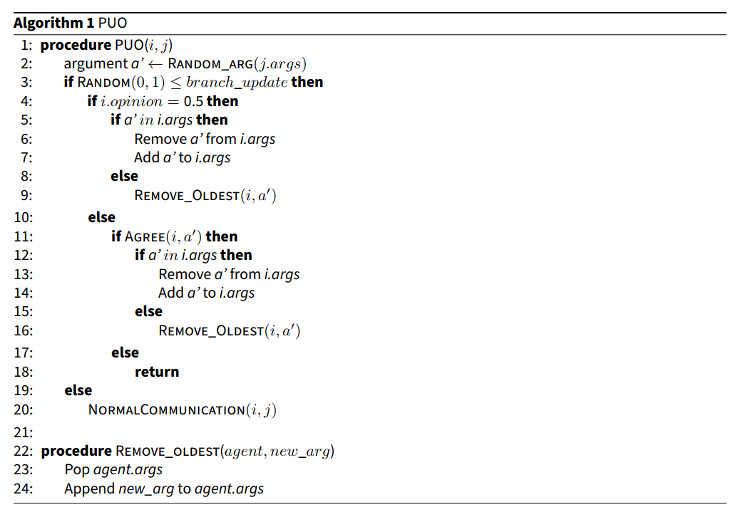
As for \(PCO\), this is a very oriented updating policy, which may easily be labelled a form of dogmatism (Kelly 2008), or worse as irrational. Despite this label, regarding \(PUO\) as a tendency rather than a deterministic attitude, it is natural to interpret it, from a more neutral standpoint, just as a simple way to operationalize some form of myside bias contributing to epistemic vigilance. Again, we achieve this by making the strength of such bias vary with the value of the parameter \(P(PUO)\). Alternatively, the counterpart of \(PCS\) is the following:
- Preferential discarding of weaker arguments (PUW): at time \(t\), the receiver \(i\) discards the oldest argument among those that are weaker, according to function \(s_{\mathbf{S_{j,t}}}\), in their individual knowledge base. (See Algorithm 2)
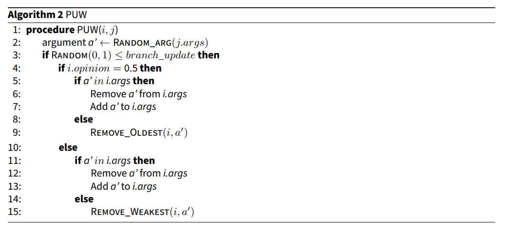
In analogy with \(PCS\), here arguments are rejected on the basis of how weak they are as far as the agent can judge.
Although for different reasons, both \(PUO\) and \(PUW\) presuppose only discarding some arguments. However, experimental evidence shows that very often, information is not simply either accepted or obliterated. People tend to rationalize their opinion or choices by backing up articulated justificatory reasons (Nisbett & Wilson 1977). If duly deceived, they do so even for choices they did not actually make and opinions they do not actually hold (Hall et al. 2012). Such a tendency suggests the possibility of a more proactive way to update one’s opinion, one allowing individuals to find new reasons, in our case arguments, when they meet information against their own opinion. Indirect evidence is provided also by the so-called backfire effect (Nyhan & Reifler 2010). When confronted with strong evidence disconfirming some false belief, individuals end up holding such a belief more strongly, by bringing the evidence into doubt. Again, contrary to well-established prejudices, this ‘creative’ tendency is by no means a sign of psychological distress, nor is typical of specific socio-cultural environments, but affects more or less everybody, including beautiful minds and Nobel laureates (Mercier & Sperber 2017, Chapter 14) and (Brotherton 2015, Chapter 11). These considerations suggest the possibility of a more articulated process of information update. One simple way of implementing this, with no strong claim of empirical adequacy, is the following:
- Vigilant update with n new arguments (VUn): when receiving an argument \(a\) that is not in line with his opinion \(o_{i,t}^{*}\), receivers \(i\) incorporates \(a\) in their individual knowledge base, together with \(n\) other arguments favouring their opinion (possibly attackers of \(a\), if any) and then discards \(n+1\) oldest arguments. (See Algorithm 3)
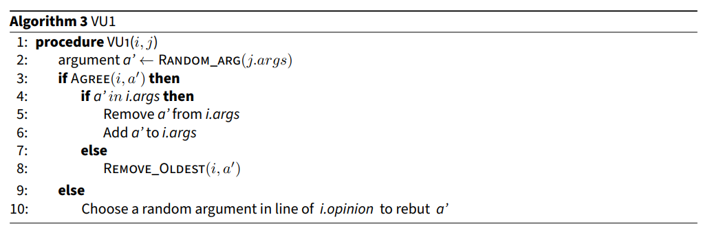
Here, the agent simply counterbalances dissonant information with arguments that favour their opinion, and the parameter \(n\) indicates how strongly. In our implementation, these \(n\) arguments are added as more recent than the argument received, thus making the confirmation bias arguably more strong. Here there are two options concerning where to select these \(n\) arguments. The agent can either, ‘fish’ them from the full repository of the global knowledge base \(\mathbf{G}\), or else from the more limited one of arguments that are still circulating. The first case is more akin to what we intuitively understand as a process of finding information by individual inquiry, while the second corresponds more to asking someone else for confirmation. In our setup we let the agent pick arguments from the whole \(\mathbf{G}\), therefore simulating individual inquiry. As a consequence, simulations take more time but provide the agents with more resources to resist consensus. Note that \(VUn\), thus conceived, can be implemented in sequential combination with \(PUO\) and \(PUW\), i.e., the receiver first integrates \(n+1\) new arguments and then selects which ones to keep as dictated by \(PUO\) or \(PUW\). This is yet another type of informational bias to be studied on a simulative basis, as we do in the next section.
Experimental Setup and Results
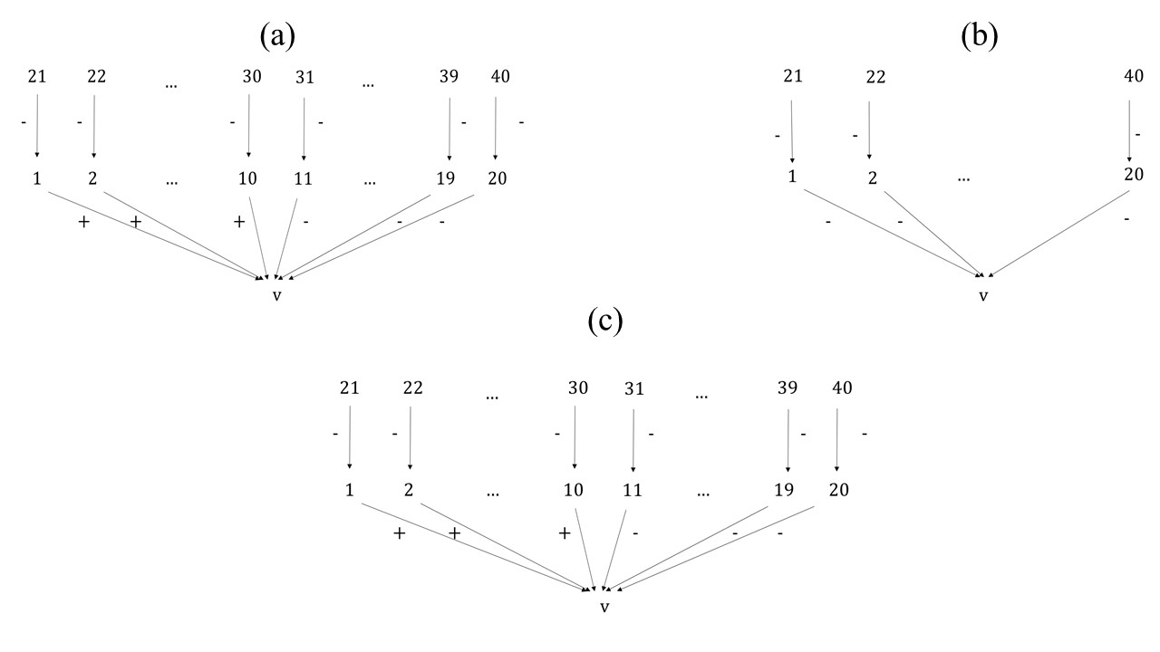
For our experiments, we set up a society of \(n = 20\) agents with different initial configurations of the global knowledge base \(\mathbf{G}\) – shown in Figure 3(a)-(c) – all with 41 of nodes, including the topic node \(v\) and 40 nodes representing arguments linked to it. Importantly, all configurations have the same number of pro and con arguments, i.e., \(Pos_{\mathbf{G}}(v) = Neg_{\mathbf{G}}(v) = 20\). Relative to the number of agents and positive and negative arguments, the parameters are the same as in Mäs & Flache (2013). However, configurations of \(\mathbf{G}\) have different topologies, so that the strength \(s_{\mathbf{G}}(v)\) of the topic node relative to the global knowledge base may vary from one case to another. The cardinality \(\vert S_{i,t}\vert\), i.e., the number of arguments relevant for the opinion of agent \(i\) at \(t\), is also set as a parameter at the beginning of each simulation run, with values \(\vert S_{i,t}\vert = 4, 6\) or \(8\). Given \(\vert S_{i,t}\vert\) – and assuming, as we do here, that each argument belongs to either \(Pos_{\mathbf{G}}(v)\) or \(Neg_{\mathbf{G}}(v)\) but not both – there are \(\vert S_{i,t}\vert + 1\) possible distributions of relevant pro and con arguments for each agent. For all runs, we randomly attributed one such configuration to each agent, and then assigned them a number of arguments from \(Pos_{\mathbf{G}}(v)\) and \(Neg_{\mathbf{G}}(v)\) that fits the configuration. For each of our tests we performed a number of runs sufficient to establish our estimates within a sufficiently small 95% confidence interval (in most cases 500 runs, but sometimes less).
As mentioned in Section 3, there are two possible equilibria, i.e., perfect consensus and maximal bipolarization. For the sake of minimizing time, the halt condition of our system was triggered as soon as either (a) the number of arguments circulating was less than \(2 \times \vert S_{i,t}\vert\), or (b) at a given time \(t\), for each agent \(i\), \(o_{i,t}^{*} = 0\) or \(o_{i,t}^{*} = 1\). Otherwise, the run stopped after \(6m\) steps. In the original model and with \(h \geq 1\), conditions (a) and (b) entail that one of the two equilibria is bound to occur, i.e., perfect consensus in case (a) or maximal bipolarization in case (b). This is not exactly the case when \(h = 0\) , as for many of our setups, or when vigilant update is implemented (Section 3.16).12 However, we checked that these halt conditions were sufficient to guarantee that the outcome of each run was stable in the limit, and this was accurate enough for our purpose.
Answering Question 1: The role of argument strength
Our first task (Question 1 of Section 1) was to investigate whether stronger reasons for a positive (resp. negative) attitude towards \(v\) could influence bi-polarization dynamics, e.g., by inducing more general consensus for (resp. against) \(v\) or, in case of a group split, by determining larger clusters of agents with a favourable (resp. negative) attitude. For this purpose, we confronted the configurations 1 and 2 of the global knowledge base (Figure 3(a) and 3(b)). Configuration 1 is a star tree, which in fact reduces to the configuration of the original ACTB environment, and therefore should give similar results. In Configuration 2 we still have an equal number of \(Pos_{\mathbf{G}}(v)\) and \(Neg_{\mathbf{G}}(v)\) arguments, but with 20 direct attackers and 20 defenders of \(v\) (each one attacking one attacker). According to our measure, the second configuration provides more support for \(v\). Indeed, the strength \(s_{\mathbf{G}}(v)\) is 0.5 for Configuration 1 while it is 0.75 for Configuration 2.
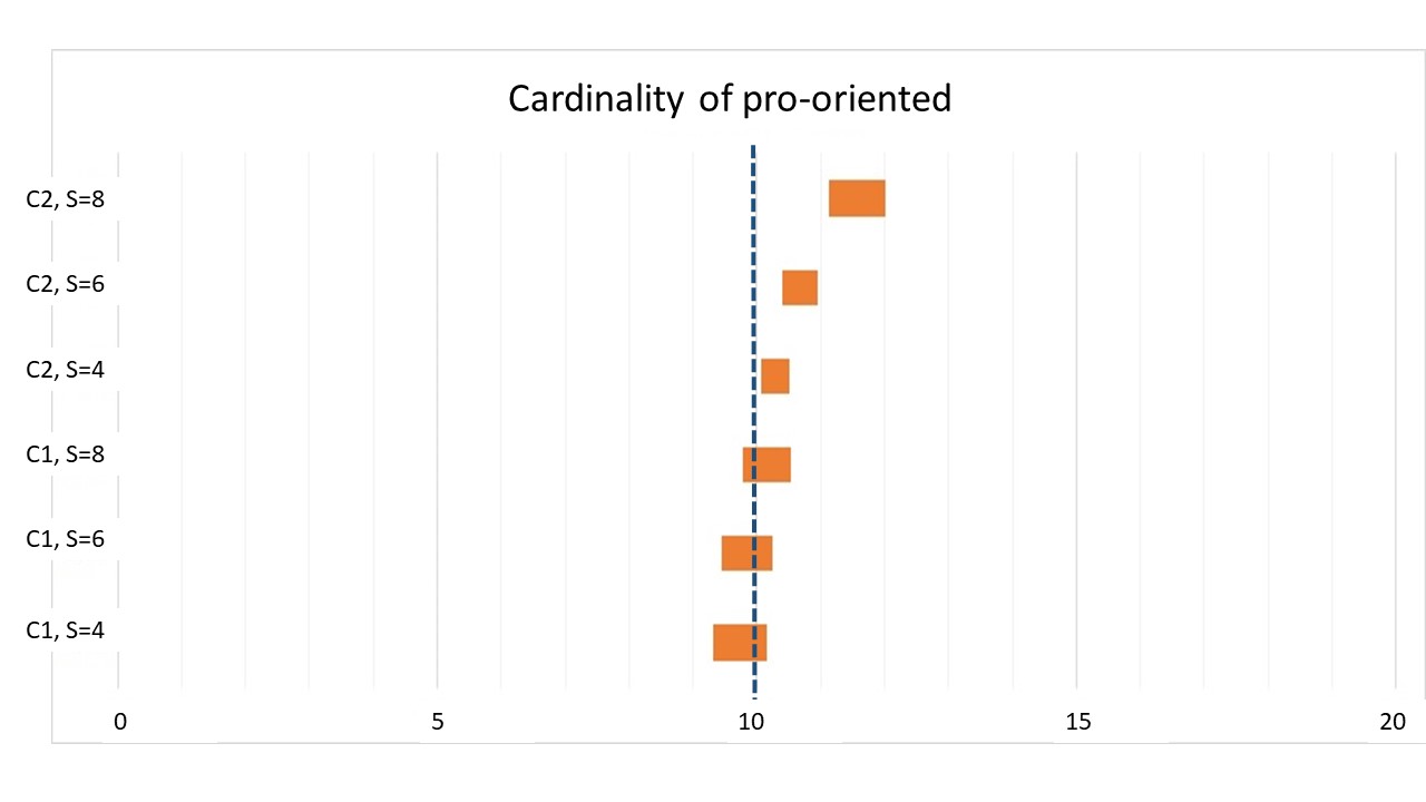
As a preliminary step we checked that with Configuration 1, our environment behaved as the original ACTB model. We therefore ran a first batch of two simulations by setting the homophily to \(h = 0\) and the agents memory to \(\vert S_{i,t}\vert = 4\) and \(= 6\) and checked that no bi-polarization effects emerged out of 500 simulations, while the average global opinion after reaching consensus was around \(0.5\) (i.e. including \(0.5\) within a small 95% confidence interval). We then ran three simulations with \(h = 9\) and the memory of the agents with values of \(\vert S_{i,t}\vert = 4\), \(= 6\) and \(= 8\). Here, as in Mäs & Flache (2013) bi-polarization effects emerge quite frequently. However, we noticed that the agent’s memory had a strong impact on the bi-polarization rate – it was inversely correlated with it – since the rate of bipolarizations drops from 97% with \(\vert S_{i,t}\vert = 4\) to 80% with \(\vert S_{i,t}\vert = 6\) and even more to 44% with \(\vert S_{i,t}\vert = 8\). Consistently with this, bi-polarization obtained more rapidly when agents have less memory, taking an average of ~700 time steps with \(\vert S_{i,t}\vert = 4\), ~2500 time steps with \(\vert S_{i,t}\vert = 6\), and ~32000 time steps with \(\vert S_{i,t}\vert = 8\). The intuitive explanation for this, as is suggested by the analytics of single runs, is that agents with less memory are more easily tilted towards the external sides of the opinion spectrum. When this happens, they are less likely to communicate with agents with an intermediate or opposite opinion. Indeed, with \(\vert S_{i,t}\vert = 4\) only 5 different degrees of opinion are possible in Configuration 1, by simple combinatorics, and each of them is significantly distant from its closest ones (0.25). By consequence, homophilous communication takes over and arguments for the other side are more easily “forgotten” during interaction. This is less likely to happen with \(\vert S_{i,t}\vert = 8\), where 9 different degrees of opinion are represented, with intervals of 0.125, to the effect that the power of homophily is significantly milder. As expected, when bipolarization occurs, groups have equal sizes. E.g., the estimated average number of pro-oriented agents for \(\vert S_{i,t}\vert = 4\) is \(9.73\) over \(20\), but with a confidence interval of 95% of diameter \(t = 0.41\), which includes \(10\). The situation is analogous for \(\vert S_{i,t}\vert = 6\) and \(\vert S_{i,t}\vert = 8\) (see Figure 4).
To answer Question 1, we compared these results with those provided by setting \(\mathbf{G}\) as in Configuration 2 under the same initial conditions, with \(h = 9\) and the same values of \(\vert S_{i,t}\vert = 4\), \(= 6\) and \(= 8\) (3 tests). Here, we obtained rates of bi-polarization outcomes of respectively, 95% for \(\vert S_{i,t}\vert = 4\), 73% for \(\vert S_{i,t}\vert = 6\) and 31% for \(\vert S_{i,t}\vert = 8\). The respective average time steps by which such scenarios end in bipolarization were the same order of magnitude of their counterparts in Configuration 1. Compared to Configuration 1, these percentages seem to witness an increasing tendency towards consensus as the memory of the agents grows. An explanation of this fact is that in Configuration 2 combinatorics allow more intermediate degrees of opinion for agents. For example, an agent owning 7 pro and 1 con argument, but where the latter is attacked by a pro, will have an opinion of 0.9375, which is not possible in Configuration 1. As noticed above, the consequence is that homophily had a diminished effect.
Despite the value of \(s_{\mathbf{G}}(v)=0.75\), the average opinion when consensus occurs was around 0.5, slightly but not meaningfully above. However, the clearest difference w.r.t. from the previous scenario was that in cases of bi-polarization, the average size of the group of pro-oriented agents increased appreciably. Indeed, it rose from \(10.28\) for \(\vert S_{i,t}\vert = 4\) to 10.68 for \(\vert S_{i,t}\vert = 6\) and 11.56 for \(\vert S_{i,t}\vert = 8\). All these values were above the mean statistically significantly (see Figure 4).13 Therefore, we can conclude, with a reasonably high degree of confidence, that a stronger \(s_{\mathbf{G}}(v)\) influences opinion dynamics in a relevant way and that our first question can, at least for its second part, be answered positively. Again, an explanation for this is provided by combinatorial considerations. In Configuration 2 the possible degrees of opinion were not symmetrically distributed and were more densely situated towards the positive side of the opinion spectrum. Following the previous example, one agent may well have an opinion of degree 0.9375 but not the symmetric one of 0.0625. This seems to be the reason why the positive side works as a stronger attractor in Configuration 2.
Answering Question 2: The role of informational biases
The second issue we aim to explore (Question 2) was whether bi-polarization could occur, or at least be fostered, as the effect of biases related to epistemic vigilance as those in Section 3. To test this, we brought homophily down to \(h = 0\) or \(h = 1\) for most of the simulation batches of this section – realising that under the conditions of the standard model of ACTB no bipolarization occurs when \(h < 3\) (Mäs & Flache 2013 p. 8).
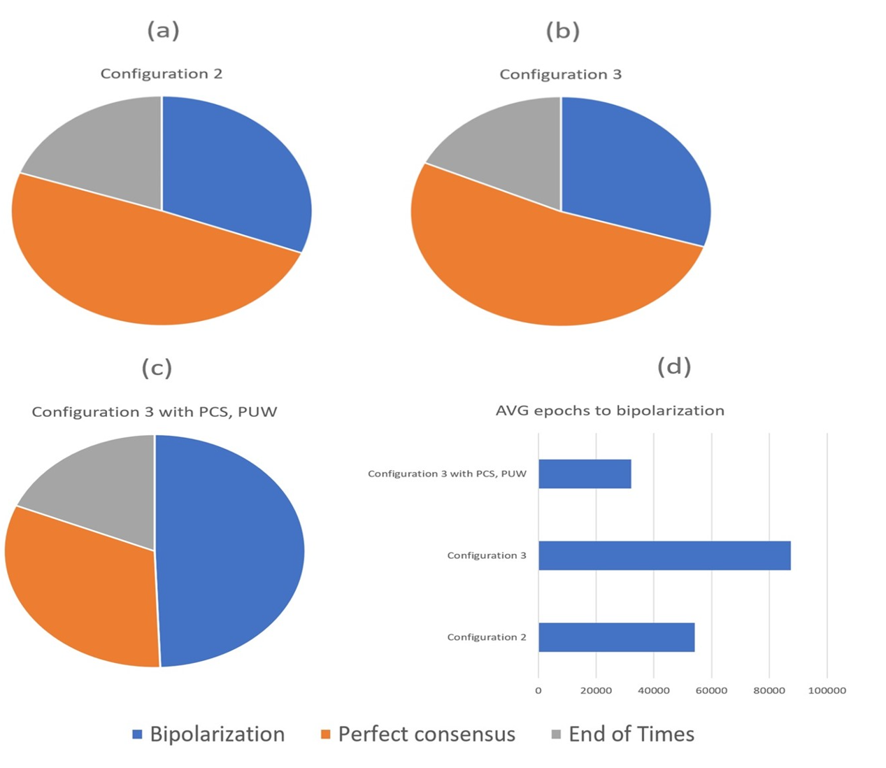
As an initial step, we tested whether arguably reasonable biases of communication and update such as \(PCS\) and \(PUW\) (Section 3.3) have any impact. Here, we used Configuration 3 (Figure 3c) as the initial setup of \(\mathbf{G}\), since in Configuration 1, these processes are indistinguishable from the standard protocol of communication and update we had employed this far. With Configuration 3 we could assess the impact of \(PCS\) and \(PUW\) while still having \(s_{\mathbf{G}}(v) = 0.5\), and therefore perfect equilibrium between \(Pos_{\mathbf{G}}(v)\) and \(Neg_{\mathbf{G}}(v)\). Here, we ran our simulations with just \(\vert S_{i,t}\vert = 8\), as this was the only scenario where the interaction between arguments and their attackers could play a sensible role.14 Preliminarily, we understood that Configuration 3 behaved comparably to Configuration 2 under the policies of communication and update of the original model.15 By implementing \(PCS\) and \(PUW\) together with no homophily, still no bi-polarization occurs as under standard conditions. Instead, with \(h=9\), the rate of bi-polarizations increased significantly (49%) and the average time to reach it dropped ($$32000 time steps). As a consequence, the combination of \(PCS\) and \(PUW\) can be hardly regarded as a sufficient cause of bi-polarization, but nonetheless works as a substantial incentive for it in the presence of homophily (Figure 5). In a nutshell, this is due to the fact that when agents are on one side of the opinion spectrum, they are more likely to receive strong arguments favouring that side and, subsequently, such arguments are more likely to attack their weaker arguments against, further boosting their opinion shift towards the favoured pole.
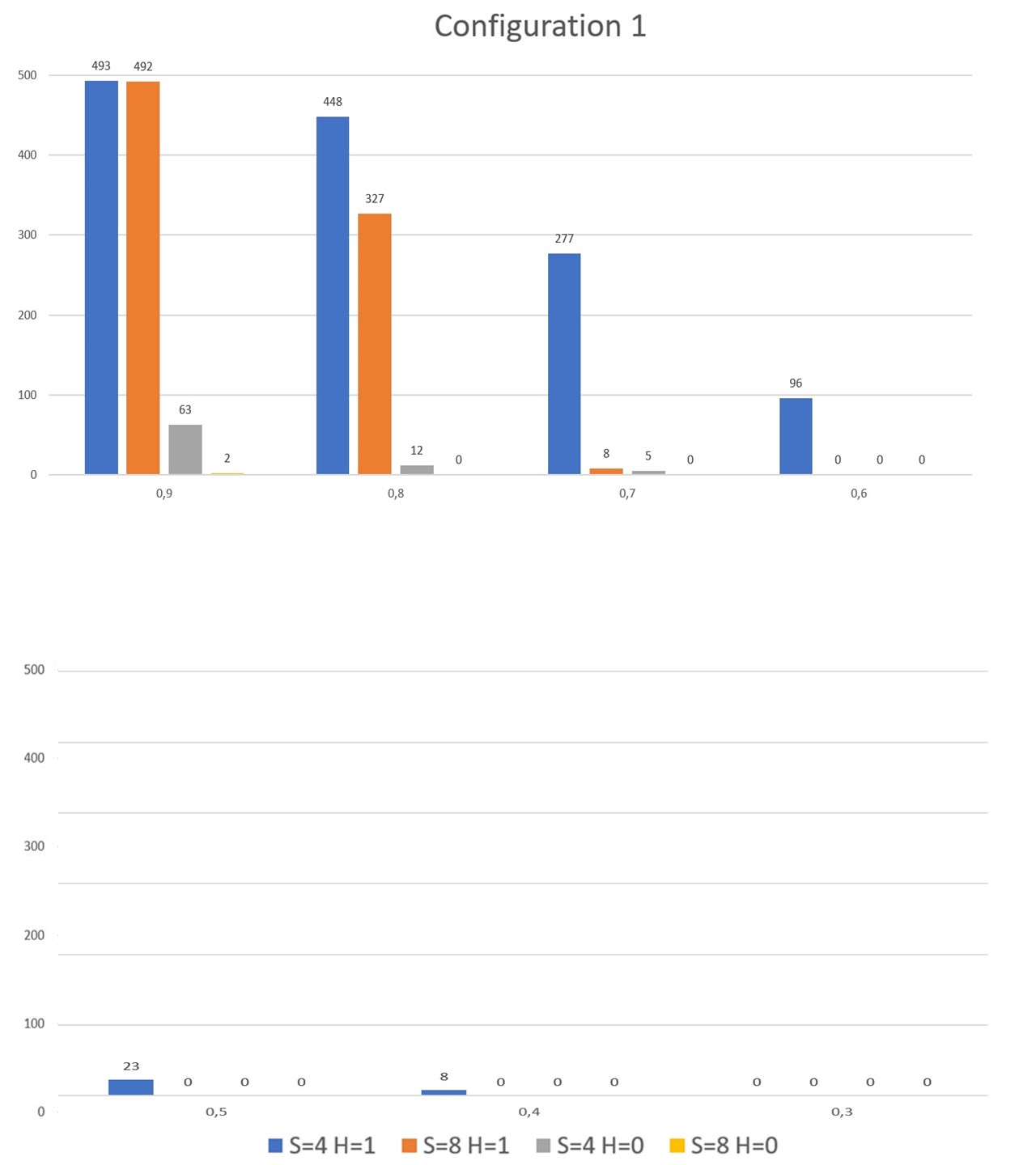
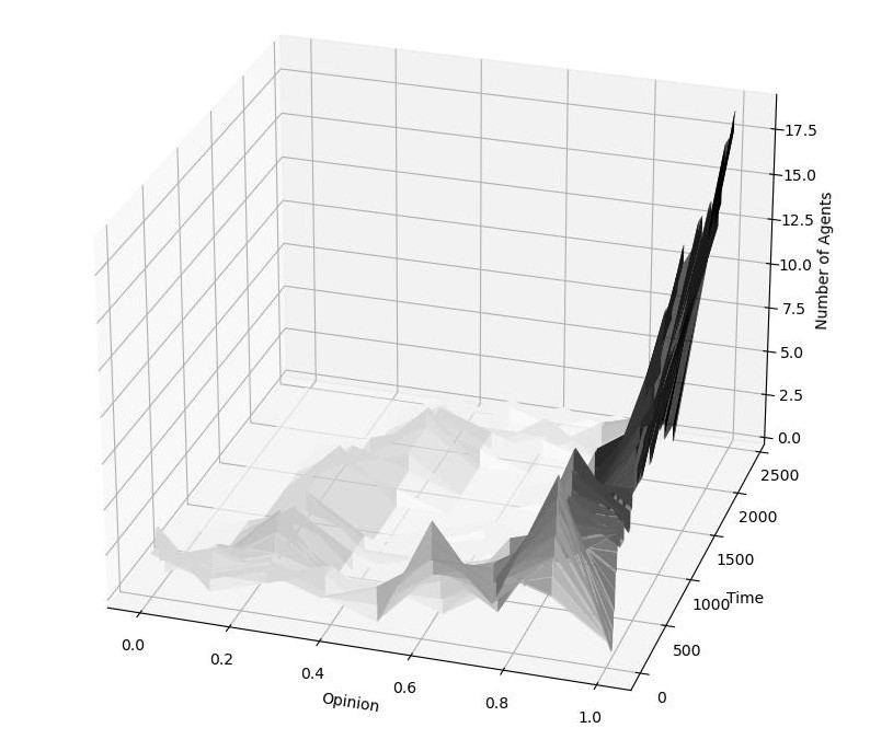
As a second step, we tested the effect of the more radical biases \(PCO\) and \(PUO\), which consisted in communicating and updating in line with one’s current opinion (Section 3.12, 3.14). For this batch of simulations, we used Configuration 1 again. As expected, by simply setting full bias in updating (\(P(PUO) = 1\)), the society always bi-polarized under any initial conditions16 and no matter what the level of homophily is, even with no bias in communication (\(P(PCO) = 0\)).17 When we also added full bias in communication (\(P(PCO) = 1\)), the process of bipolarization speeded up significantly.18 Quite surprisingly, however, the bi-polarization effects almost vanished as soon as we brought the probability of \(PUO\) and \(PCO\) slightly down. Indeed, with \(P(PUO) = P(PCO) = 0.9\), no homophily and high individual memory (\(\vert S_{i,t}\vert = 8\)) bi-polarization occurred only two times over 500 runs and with groups of radically different sizes (e.g., 19 pro against 1 con), while it disappeared with lower levels of probability for \(PUO\) and \(PCO\) (Figure 6, yellow). With a moderate degree of homophily (\(h = 1\)) bi-polarizations were instead still dominant (494 over 500), but almost disappeared as soon as \(P(PUO) = P(PCO) = 0.7\) (Figure 6, red).19. The most plausible explanation for this behaviour is that an even small probability of accepting (and communicating) arguments to the contrary enables agents to shift from one side to the other when sufficiently close to the middle. And, as soon as one group becomes dominant in number, it works as an attractor, bringing the agents of the other group one by one on its side. Figure 7 shows this dynamic at work in a specific run.
Things are only slightly different with no homophily and low individual memory (\(\vert S_{i,t}\vert = 4\)), where bi-polarization occurred 12% of the time with \(P(PUO) = P(PCO) = 0.9\), here too with groups of very different cardinality, e.g., 19 to 1 or 18 to 2 , and disappeared as soon as \(P(PUO) = P(PCO) = 0.6\) (Figure 6, grey).20 With \(h=1\) however, bi-polarizations stop at \(P(PUO) = P(PCO) = 0.3\) (Figure 6, blue). Such an increased resilience to consensus for agents with low memory was again due to the presence of bigger jumps among opinion degrees (see Section 4.4). Furthermore, It is fundamental to note that even with moderate levels of \(P(PUO)\) and \(P(PCO)\) (=0.3), consensus was almost inevitably established towards the opposite ends of the opinion spectrum, as illustrated by Figure 7.21 Thus, in the absence of homophily, dogmatic attitudes such as communicating and accepting only arguments that fit one’s own opinion may count as a strong driver of polarization, but hardly as a cause of group split. In other words, if \(PUO\) and \(PCO\) are regarded as an adequate reproduction of the workings of the myside bias, then such bias needs to be very strong for it to induce bi-polarization effects.
As a third variation, we tested whether vigilant update (Section 3.3), an alternative way of operationalizing a form of myside bias, has different bipolarizing effects. We should remember that, under \(VUn\), the agent receiving a new argument checks if the latter aligns with his opinion and, if so, adds it to his individual knowledge base in the standard way. Otherwise, the agent adds \(n\) more arguments supporting his opinion to contrast it. For all these simulations we assumed \(P(VUn)=1\). Under Configuration 1, we performed four tests with \(VU1\), \(h = 0\) or \(=1\), \(\vert S_{i,t}\vert = 4\) or \(=8\), and no bi-polarization occured. Indeed, we obtained bi-polarizations (in all runs) only with \(VU2\), \(\vert S_{i,t}\vert = 4\) and \(h = 1\). Considering that, when \(\vert S_{i,t}\vert = 4\), vigilant update with two arguments always provides half of the size of one agent’s knowledge base to counter adversary information, these tests show that only an extreme form of vigilant update can generate bipolarization by this mechanism alone. As for \(PCO\) and \(PUO\), all runs end nevertheless in polarization, with all agents having an opinion of either \(1\) or \(0\), by the same dynamics illustrated in Figure 7.
Of further interest is to test whether bi-polarization obtains by implementing \(VUn\) in combination with different levels of \(P(PUO)\), where agents perform vigilant update by adding \(n\) new arguments favouring their opinion when they receive contrary information, and then discard the contrary argument with probability \(=P(PUO)\). The rationale behind this is that it may well be the case that different forms of bias work together, at least as far as experimental evidence from studies in the psychology of reasoning would show (see Section 3). Under Configuration 1 and \(h = 0\) we performed three tests with \(VU2\), keeping \(\vert S_{i,t}\vert = 4\), and \(P(PUO) = 0.9\), \(= 0.6\) or \(= 0.3\). In the first two cases, bi-polarization always occured (500 runs over 500), although at different speeds (resp. $$200 and $$9200 time steps), while in the third case it occured 195 times over 500 with an average speed of $$2m steps (other runs exceeded the time limits but their analytics indicated a tendency towards bi-polarization). We then tried the same three tests with \(VU1\) and found that bi-polarization was always obtained with \(P(PUO) = 0.9\), still 15% of times when \(P(PUO) = 0.6\) (but with groups of very different sizes), while it did no longer occur when \(P(PUO) = 0.3\). Here, combining \(VUn\) with \(PUO\) generated group split, but only consistent levels of the latter work as efficient drivers of it.
| \(VU1\) | \(VU1\) | \(VU1\) | \(VU1\) | \(VU2\) | \(VU2\) | \(VU2\) | \(VU2\) | |
| \(P(PUO)=0\) | \(P(PUO)=.3\) | \(P(PUO)=.6\) | \(P(PUO)=.9\) | \(P(PUO)=0\) | \(P(PUO)=.3\) | \(P(PUO)=.6\) | \(P(PUO)=.9\) | |
| \(h = 0\) | no | no | 15% | 100% | eot | 100% | 100% | 100% |
| \(h = 1\) | no | 9% | 97% | 100% | 100% | 100% | 100% | 100% |
We will leave other possibly interesting combinations of parameters and further configurations for future exploration. What our simulations showed is that, in order to produce bipolarization without homophily in this model, we need to assume that strong forms of informational bias are at work. Given this, we could ask why this is so, and what is different from other simulative approaches where bipolarization is a more natural outcome. The final section discusses our results in the light of general features of the ACTB environment and then provides some comparative insights.
Discussion
Here, we have expanded the simulative model of ACTB in two different directions. On one hand, we generalized the idea of an argumentative knowledge base and consequently adapted its original measure of argument-based opinion. On the other hand, we implemented more policies of argument communication and updates. These expansions allowed us to address two research thesis on a precise simulative basis. Question 1 is about whether and how stronger arguments from one side lead to more consensus or to larger groups polarizing in this direction. As our results of Section 4 show, stronger arguments have a tangible effect only on the second of these dimensions. Question 2 asks whether bipolarization can emerge from informational biases other than homophily, as conjectured and experimentally tested by a solid tradition in social psychology. Here, the answer is moderately positive, insofar as our experiments show that, in the absence of homophily, strong forms of informational bias are needed to force bi-polarization. Indeed, when the tendency towards a biased update is less than perfect, even a small amount of noise suffices to disrupt the dynamics of bi-polarization.
Of course, our answers to questions 1 and 2 depend heavily on the simulative model adopted. We cannot pretend to generalize their importance beyond its assumptions and without empirical backup. However, the general architecture of the model can provide some useful insights relating to general findings of polarization and bi-polarization. Here, we discuss two salient aspects of the ACTB model: (a) the structure of the network of communication among agents and (b) the assumptions about the global and the individual knowledge base. More specifically, we draw some conjectures about how these features influence our results concerning Question 2. Moving from this point, we compare the ACTB model with a family of ABMs with rational (Bayesian) agents, where alternative assumptions generate different results, and with the argument-based model of Singer et al. (2019), similar in spirit to ACTB. Regarding the latter, the results point to a large extent in the same direction as ours, but our experiments in Section 4.8 - 4.12 open a different interpretation.
The network structure
In the ACTB simulation environment, bi-polarization and consensus are strongly dependent on the communication protocol and the implicit network structure generated by it. For example, as noted elsewhere (Proietti & Chiarella 2021), all other things being equal, the rate of bi-polarization outcomes diminishes significantly by inverting the roles of speaker and receiver – i.e., by first randomly choosing the speaker and then selecting the receiver by homophily. In the ACTB simulation environment, each agent can in principle communicate with every other agent and therefore the communication network is a totally connected one. However, homophily plays a major role in determining the weight of the communication channel between each pair of agents, which is inversely proportional to the similarity of their opinion. Even with a minimal degree of homophily (\(h \geq 1\)), communication between agents with mostly dissimilar opinions, is impossible. Therefore, the structure of the communication network is endogenously determined by the agents’ opinions and the two things shape each other by a back-and-forth process. As soon as opinions become more distant, the likelihood of communication diminishes, and this indirectly causes more distance in opinions …and so forth. This is another way to understand how bi-polarization emerges in the original environment. When we set \(h = 0\) instead, the network is forced to stay totally connected and all links keep equal weight. The fact that bi-polarization is extremely hard to achieve without homophily can therefore be interpreted as a confirmation of the empirical finding according to which opinions in diverse groups and in conditions of fully open discussion tend to depolarize (Abrams et al. 1990; Vinokur & Burnstein 1978).
Assumptions on the knowledge bases
Global knowledge \(\mathbf{G}\) is based on a finite set of arguments. Although the fact that available information/arguments about any topic are potentially infinite may be objected to, this does not seem to constitute a strong limitation of the ACTB model, which is still somehow realistic, provided that the size of \(\mathbf{G}\) is sufficiently large with respect to individual knowledge bases. Furthermore, dealing with a finite set of arguments allows us to calculate \(s_{\mathbf{G}}(v)\) as the opinion of an ideal mostly informed agent and therefore serves as a touchstone to evaluate group performance.
Concerning the way rational agents are modelled in this framework, we already pointed to certain specific features that make the ACTB model different from other possible approaches. First, agents have limited memory and therefore lack perfect recall, which is a reasonable assumption when dealing with bounded rationality. We have shown that the size of their memory strongly affects the rate of bipolarization outcomes under homophily. One can summarize this finding as “more memory, more consensus”. However, we found no evidence that increased consensus entails a better performance in terms of truth-tracking, i.e., having the average opinion of the group closer to \(s_{\mathbf{G}}(v)\).
Furthermore, in the original model the size of the agents’ memory is kept constant by discarding older arguments. With our new updating policies some further mechanisms of preferential discarding are introduced, but still the main factor is how old arguments are. There is room for objections about lack of realism here. Indeed, for real individuals, pieces of information are not all on a par, some are more firmly grounded in their cognitive life and more resilient to change, while others are evanescent. However, hardcoding this into agents’ informational behaviour amounts to the assumption of yet another strong form of informational bias. Related to this is a further assumption, i.e., that the agents’ opinion, as in the original model, is fully determined by the arguments an agent owns at any given time, and not by the full stream of its previous evidence. This may determine big jumps in opinion after any updates of information, again proportional to the size of the agent’s memory. As shown in Proietti & Chiarella (2021), there are other ways of defining argument strength that take into account previous evidence and that make the agent’s opinion more resilient, thus mitigating the effect of big jumps. Arguably however, such resilience can again, be regarded as a form of bias, as it makes the agents’ opinion strongly dependent on initial (arbitrarily determined) conditions. Be this as it may, it is an interesting task to explore how these general features of the environment influence its outcome that we leave for future work. For the present discussion, we will limit ourselves to a brief comparison with alternative agent-based approaches.
A comparison with Bayesian frameworks
The fact that strong informational biases are necessary to generate bi-polarization effects in the absence of homophily seems at odds with the results obtained by Pallavicini et al. (2021) using the Laputa multi-agent simulation environment (Angere 2010; Olsson 2011). In Laputa, agents exchange information about a given proposition \(p\). They do so by sending a binary message about its truth, either \(p\) or \(\neg p\). Upon receiving new information, agents revise their degree of belief of \(p\) by means of a standard mechanism of Bayesian update. Here, updating the likelihood of a given hypothesis \(H\) upon receiving new data \(D\) has the general form \(P(H \mid D) = \frac{P(D \mid H)P(H)}{P(D)}\), where \(P(A \mid B)\) is the conditional probability of \(A\) given \(B\). Here, the revised degree of belief about \(p\) after acquiring new information (\(P(H \mid D)\)) is a function of, essentially, the agent’s prior opinion (\(P(H)\)) and their trust in the source telling the truth \((P(D \mid H))\). It turns out that under a large variety of initial conditions and distributions of trust among agents, bi-polarization occurs in a situation of fully open communication and by a mechanism of prima facie fully rational updates.
Here, we cannot provide a detailed comparison of our model and Laputa, since the added dimension of trust makes system behaviour harder to reconstruct, let alone to explain. One key however, are some fundamental observations by Jern et al. (2014) concerning the behaviour of Bayesian agents in the context of the closely related phenomenon of belief polarization. The latter is understood as the process by which two individuals with different prior beliefs observe the same external evidence and subsequently strengthen their beliefs in opposite directions. Jern et al. (2014) showed that this type of contrary updating is fully compatible with a Bayesian framework. Indeed, if two agents have different prior stances on an hypothesis \(H\) and assume different conditional probability distributions for how \(H\) influences the observed data \(D\), then the same evidence can update stance in opposite directions. Contrary updating may also occur when further background knowledge besides \(H\), an additional random variable \(V\), influences data observation in any specific ways. There, contrary updating may occur even if two agents agree on the conditional probability of \(D\) given \(H\) and \(V\), provided that they assign different priors to \(H\) and \(V\). In the Laputa environment, trust in the source seems to play such a role and therefore allows for contrary updating that ultimately leads to bi-polarization. In the standard protocol of ACTB contrary updating is simply not possible, since each new argument is accepted and its polarity determines the direction of the update. New procedures such as \(PCO\) and \(VUn\) on the other hand, open up to the possibility of contrary updating given the same evidence (argument), and this seems to explain why groups can bi-polarize even in the absence of homophily. However, nothing similar to background knowledge \(V\) is at work here, since all arguments are on a par and each one is discarded when it gets sufficiently old. As mentioned, it is possible that the memory of actual individuals works in a significantly different way. More insights on this issue would provide fuel for future research.
A comparison with the model of Singer et al. (2019)
Very similar in spirit to our framework is the multi-agent model by Singer et al. (2019). Here too, each agent owns a limited size22 set of pro and con arguments and their opinion is fully determined as a weight of their strengths. One main difference with respect to our model is that weights are assigned as arbitrary numerical values, normally distributed around 0, negative for pro and positive for con, and therefore arguments are regarded as independent of each other. As in our case, interaction consists of an exchange of arguments. Different from our setup, here, communication is not one-to-one but one-to-many (the sender communicates one of its arguments to everyone else) and there is no homophilous selection of the interaction partner.
The effect of different updating policies is put to test. A first policy is the so-called naive-minded one, where agents receiving a new argument, dismiss one of the oldest arguments they have in their repository. With some provisions, this policy is the same as the standard update protocol of the ACTB model. Not surprisingly, bi-polarization does not occur with this policy, in line with what previously shown by Mäs & Flache (2013) in the absence of homophily. A second policy is the so-called weight-minded, where agents receiving a new argument discard the weakest one in their repository. In spirit, this is the same as our \(PUW\). In this case, our results for \(PUW\) (and \(PCS\)) confirm theirs. The possibility of introducing homophily as a parameter in our setup shows, however, that such a policy can nonetheless act as a booster for bi-polarization under favourable conditions.
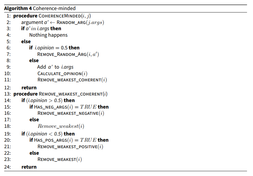
A third update policy is the coherence-minded. Here, the agent receiving a new argument dismisses the weakest one from those contrary to their opinion. At first sight, this looks almost the same as our \(PUO\), but with a caveat. While \(PUO\) encodes the ‘dogmatic’ attitude by which agents discard some argument a priori when it goes against their prior opinion, in the coherence-minded policy they provisionally accept the new argument, recalculate their opinion by adding it to the balance, and then decide which argument to discard on the basis of the revised opinion. Moving from this, Singer et al. (2019) argue that the coherence-minded policy fulfils the desiderata for a rational updating policy. And since bi-polarization is a dominant outcome under this policy in their experimental setup, they conclude, as one main claim of their work, that bi-polarization is consistent with rationality.
However, as we have suggested, in models of this type bi-polarization occurs if agents cannot switch sides in the opinion spectrum when exposed to contrary information. In this case, it seems that this possibility is directly proportional to (a) the size of their memory, with more arguments, adding one does not make a big difference, and (b) the distribution of the numerical weights of the arguments, if all arguments have similar strength, adding one is less likely to shift the balance. Therefore, it is quite possible that the bi-polarization effects in the coherence-minded setup are induced by the very same dynamic occurring when \(P(PUO) = 1\). To check this, we coded the coherence-minded update (Algorithm 4) and tested it in our model under the same parameters that we used for the experiments with \(P(PUO) = 1\). Both with \(\vert S_{i,t}\vert = 4\) and \(\vert S_{i,t}\vert = 8\) results are univocal: bi-polarization occurs 100% of the times (over 500 runs) in both cases, and the analytics show that opinion shift happens very rarely. It is likely that this is due to the fact that our setup is particularly unfavourable with regard to conditions (a) and (b). The agents’ memory is sufficiently large and all arguments have equal weight in Configuration 1. To make conditions more favourable for opinion shift, we also tried with a reduced memory of \(\vert S_{i,t}\vert = 3\) and results are the same.
In sum, it may well be the case that this happens because our setup and that of Singer et al. (2019) are not able to tell the workings of the coherence-minded policy from those of \(PUO\). This becomes more intriguing when compared to our results for \(P(PUO) = 0.9\). There, although the bias is stronger, the noise created by an even small probability of accepting new information at face value is sufficient to induce opinion shifts, and therefore consensus (in fact polarization) in the long run.
Notes
We would like to thank Referee 2 for referring us to this work, of which we were not aware of before submission.↩︎
This is a common assumption with many models based on imitation such as DeGroot (1974).↩︎
The effect of homophily is indeed similar to what occurs when individuals, as a result of ingroup/outgroup division, tend to communicate only with members of their group, with the difference that here group divides are not exogenously determined from the beginning, but emerge as the effect of homophilous communication.↩︎
This reflects the fact that we are dealing with non-omniscient agents. In this simulation environment, this assumption is also crucial to obtain bi-polarization effects. If dropped, all agents’ individual knowledge bases would coincide in the long run with the global knowledge base and therefore their opinions would converge.↩︎
This holds by assuming that the initial opinions are uniformly distributed along the opinion spectrum, as it is the case in our setup.↩︎
In the original model of ACTB the measure ranges between \(-1\) and \(+1\) and is calculated as
\[\frac{\sum_{a \in (S_{i,t}\cap Pro(v))}we(a) - \sum_{a \in (S_{i,t}\cap Con(v))}we(a)}{\vert S_{i,t} \vert}\] \[(3)\] Equation 2 is simply a linear transformation of this, implemented for the practical purpose of scaling all measures on the same interval \([0,1]\).↩︎
Assuming that individual knowledge bases are proper induced subgraphs of \(\mathbf{G}\) comes with a number of implicit assumptions of the agents’ capacities. For example, agents cannot mistakenly believe that one argument attacks another when it does not (in \(\mathbf{G}\)). However, these assumptions are not problematic for our investigation.↩︎
To the best of our knowledge the only definition of an argument strength measurement for general directed graphs (possibly containing cycles) is by Leite & Martins (2011). However, it was shown by Amgoud et al. (2017) that this approach suffers from technical issues that prevent its generalization.↩︎
We should note however, that many real-life debates have genuine dilemmas, which are typically represented as cycles of attacks between arguments. For this reason, measurements of argument strength for general graphs are desirable.↩︎
It would seem natural to define our measure \(s_{\mathbf{S_{i,t}}}\) relative only to the graph \(\mathbf{S_{i,t}}\). As mentioned, the issue is that in the individual knowledge base \(\mathbf{S_{i,t}}\) arguments that are not directly linked to the topic node \(v\) in G are likely to be disconnected from it and therefore would have no impact on the calculation of its strength. Let us suppose that \(b R_{\mathbf{G}}^{-} a_{1} R_{\mathbf{G}}^{-} v\) but \(a_{1} \not\in S_{i,t}\). In such a case, \(b\) counts as an argument with negative influence on \(v\) relative to \(\mathbf{G}\) but not to \(\mathbf{S_{i,t}}\), and therefore would not affect the strength of \(v\). Although this may be reasonable in certain contexts, it is objectionable in many others. For our experiments we decided to include these arguments in our calculations. However, this feature can easily be modified as a parameter of the model.↩︎
One straightforward alternative is to calculate the strength of each argument only locally, i.e., weighting only its direct attackers and supporters, and not its more distant ancestors. This amounts to replace \(Pos(a)\) with \(Pro(a)\) and \(Neg(a)\) with \(Con(a)\) in Equation 3. Otherwise, instead of summing the cardinalities of positive and negative arguments in the denominator, one may sum up their strengths, so to obtain equation
\[\frac{\sum_{b \in S_{i,t}\cap Pos_{\mathbf{G}}(a)}s_{\mathbf{S_{i,t}}}(b) - \sum_{b \in S_{i,t}\cap Neg_{\mathbf{G}}(a)}s_{\mathbf{S_{i,t}}}(b)}{\sum_{b \in Pos_{\mathbf{G}}(a) \cup Neg_{\mathbf{G}}(a)}s_{\mathbf{S_{i,t}}}(b)}\] \[(6)\] . This would also provide a well-defined measurement, consistent with \(o_{i,t}\) as previously mentioned.↩︎
Indeed, with \(h = 0\) condition (b) does not entail that bi-polarization is stable, since communication is still possible between maximally dissimilar agents lying at the opposite poles of the opinion spectrum. On the other hand, if vigilant update is active as described in Section 3.16, then arguments that have been forgotten can possibly circulate again, and therefore condition (a) does not guarantee that opinions will converge.↩︎
Despite deviations from the mean did not seem to be very high, one should take into account the small number of agents (\(= 20\)) of our setup, as well as the fact that the measurements we adopted determines only an moderate unbalance (\(s_{\mathbf{G}}(v) = 0.75\)) compared to other possible measures of topic strength (see e.g., fn. 11) where the strength of the topic node would instead be 1.↩︎
With less memory, e.g., with \(\vert S_{i,t}\vert = 4\), it was highly unlikely for some agent to own both one argument and its attacker in his individual knowledge base.↩︎
Here, no bi-polarization occurred with and \(\vert S_{i,t}\vert = 8\) no homophily, while with \(h = 9\) we obtained 30% of bi-polarization outcomes, i.e., a rate comparable to that of Configuration 2 (see Section 4.1). Average cardinality of pro-oriented agents was approximately 10, as expected, and time needed to reach bi-polarization is $$87000 time steps.↩︎
More precisely we ran our tests on a \(2 \times 2 \times 10 \times 10\)-element space where \(\vert S_{i,t}\vert = 4\) or \(= 8\), \(h = 0\) or \(=1\), and \(P(PUO)\) and \(P(PCO)\) have values increasing by \(0.1\) from \(= 0\) to \(1\).↩︎
This outcome is indeed almost analytical, since agents starting with an oriented opinion will always discard information while on the contrary, agents in the middle (\(o_{i,t}^{*} = 0.5\)) will do the same as soon as their opinion shifts in one direction as the effect of argument communication. See also Kelly (2008).↩︎
For example, with \(h=0\), \(\vert S_{i,t}\vert = 8\) and \(P(PUO) = P(PCO) = 1\) reached maximal bi-polarization on average ~900 time steps, much faster compared to ~5500 steps with \(P(PCO) = 0\).↩︎
Bi-polarizations were 327 over 500 with \(P(PUO) = P(PCO) = 0.8\), only 8 with \(P(PUO) = P(PCO) = 0.7\), and none with \(P(PUO) = P(PCO) = 0.6\).↩︎
More precisely, bi-polarization occurred 12 times over 500 when \(P(PUO) = P(PCO) = 0.8\) and 5 times when \(P(PUO) = P(PCO) = 0.7\). Furthermore, the impact of \(PCO\) was negligible in all these cases, since, e.g., bi-polarization still occurred 10% of the times when \(P(PUO) = 0.9\) and \(P(PCO)= 0\), very similar compared to 12% with \(P(PCO)= 0.9\).↩︎
This comes as no surprise, since, as soon as the whole community is brought on the same side of the opinion spectrum, then the specific workings of \(PCO\) and \(PUO\) force to circulate and keep alive only arguments in the same direction, while ‘killing’ arguments to the contrary.↩︎
Singer et al. (2019) also run some experiments where agents have an unlimited memory and cumulate information without ever discarding arguments. There consensus is always obtained. Rephrased in our terms, this result is a consequence of the fact that agents end up being omniscient, since their individual knowledge bases become the same as the global knowledge base and therefore identical to each other, as we pointed out in footnote 3.↩︎
Acknowledgements
Special thanks to Referee n. 2 for insightful comments that helped improving the final version of this work. We also wish to thank Ilaria Jemos for technical support. The infrastructure for the simulative part of this work was provided by the GARR Consortium. This work was carried out within the framework of the project "RAISE - Robotics and AI for Socio-economic Empowerment” and has been supported by European Union - NextGenerationEU.
Disclaimer
Funded by the European Union - NextGenerationEU. However, the views and opinions expressed are hose of the authors alone and do not necessarily reflect those of the European Union or the European Commission. Neither the European Union nor the European Commission can be held responsible for them.
References
ABRAMS, D., Wetherell, M., Cochrane, S., Hogg, M. A., & Turner, J. C. (1990). Knowing what to think by knowing who you are: Self-categorization and the nature of norm formation, conformity and group polarization. British Journal of Social Psychology, 29(2), 97–119. [doi:10.1111/j.2044-8309.1990.tb00892.x]
AMGOUD, L., & Ben-Naim, J. (2016). Evaluation of arguments from support relations: Axioms and semantics. 25th International Joint Conference on Artificial Intelligence (IJCAI 2016). [doi:10.24963/ijcai.2018/720]
AMGOUD, L., Bonzon, E., Correia, M., Cruz, J., Delobelle, J., Konieczny, S., Leite, J., Martin, A., Maudet, N., & Vesic, S. (2017). A note on the uniqueness of models in social abstract argumentation. arXiv preprint. Available at: https://arxiv.org/abs/1705.03381.
ANGERE, S. (2010). Knowledge in a social network. Available at: https://lucris.lub.lu.se/ws/files/6180842/4393835.pdf.
BANISCH, S., & Olbrich, E. (2021). An argument communication model of polarization and ideological alignment. Journal of Artificial Societies and Social Simulation, 24(1), 1. [doi:10.18564/jasss.4434]
BARON, J. (2000). Thinking and Deciding. Cambridge: Cambridge University Press.
BARONI, P., Rago, A., & Toni, F. (2019). From fine-grained properties to broad principles for gradual argumentation: A principled spectrum. International Journal of Approximate Reasoning, 105, 252–286. [doi:10.1016/j.ijar.2018.11.019]
BERGER, J., & Heath, C. (2008). Who drives divergence? Identity signaling, outgroup dissimilarity, and the abandonment of cultural tastes. Journal of Personality and Social Psychology, 95(3), 593. [doi:10.1037/0022-3514.95.3.593]
BRAMSON, A., Grim, P., Singer, D. J., Berger, W. J., Sack, G., Fisher, S., Flocken, C., & Holman, B. (2017). Understanding polarization: Meanings, measures, and model evaluation. Philosophy of Science, 84(1), 115–159. [doi:10.1086/688938]
BROTHERTON, R. (2015). Suspicious Minds: Why We Believe Conspiracy Theories. London: Bloomsbury Publishing. [doi:10.5040/9781472944528]
CAYROL, C., & Lagasquie-Schiex, M.-C. (2005). Graduality in argumentation. Journal of Artificial Intelligence Research, 23, 245–297. [doi:10.1613/jair.1411]
CAYROL, C., & Lagasquie-Schiex, M.-C. (2009). Bipolar abstract argumentation systems. In G. Simari & I. Rahwan (Eds.), Argumentation in Artificial Intelligence (pp. 65–84). Berlin Heidelberg: Springer. [doi:10.1007/978-0-387-98197-0_4]
DEFFUANT, G., Neau, D., Amblard, F., & Weisbuch, G. (2000). Mixing beliefs among interacting agents. Advances in Complex Systems, 3(01n04), 87–98. [doi:10.1142/s0219525900000078]
DEGROOT, M. H. (1974). Reaching a consensus. Journal of the American Statistical Association, 69(345), 118–121. [doi:10.1080/01621459.1974.10480137]
FLACHE, A., & Macy, M. W. (2011). Small worlds and cultural polarization. The Journal of Mathematical Sociology, 35(1–3), 146–176. [doi:10.1080/0022250x.2010.532261]
HALL, L., Johansson, P., & Strandberg, T. (2012). Lifting the veil of morality: Choice blindness and attitude reversals on a self-transforming survey. PLoS One, 7(9), e45457. [doi:10.1371/journal.pone.0045457]
HEGSELMANN, R., Krause, U., & others. (2002). Opinion dynamics and bounded confidence models, analysis, and simulation. Journal of Artificial Societies and Social Simulation, 5(3), 2.
HOGG, M. A., Turner, J. C., & Davidson, B. (1990). Polarized norms and social frames of reference: A test of the self-categorization theory of group polarization. Basic and Applied Social Psychology, 11(1), 77–100. [doi:10.1207/s15324834basp1101_6]
ISENBERG, D. J. (1986). Group polarization: A critical review and meta-analysis. Journal of Personality and Social Psychology, 50(6), 1141. [doi:10.1037/0022-3514.50.6.1141]
JANIS, I. L. (1983). Groupthink. Boston, MA: Houghton Mifflin.
JERN, A., Chang, K.-M. K., & Kemp, C. (2014). Belief polarization is not always irrational. Psychological Review, 121(2), 206. [doi:10.1037/a0035941]
KELLY, T. (2008). Disagreement, dogmatism, and belief polarization. The Journal of Philosophy, 105(10), 611–633. [doi:10.5840/jphil20081051024]
KRIZAN, Z., & Baron, R. S. (2007). Group polarization and choice-dilemmas: How important is self-categorization? European Journal of Social Psychology, 37(1), 191–201. [doi:10.1002/ejsp.345]
LAZARUS, J. V., Wyka, K., White, T. M., Picchio, C. A., Gostin, L. O., Larson, H. J., Rabin, K., Ratzan, S. C., Kamarulzaman, A., & El-Mohandes, A. (2023). A survey of COVID-19 vaccine acceptance across 23 countries in 2022. Nature Medicine, 29, 1–10. [doi:10.1038/s41591-022-02185-4]
LINGLE, J. H., & Ostrom, T. M. (1981). Principles of memory and cognition in attitude formation. In R. Petty, T. M. Ostrom, & T. C. Brock (Eds.), Cognitive Responses in Persuasion (pp. 399–420). Taylor & Francis.
MÄS, M., & Flache, A. (2013). Differentiation without distancing. Explaining bi-polarization of opinions without negative influence. PLoS One, 8(11), e74516.
MERCIER, H., & Sperber, D. (2011). Why do humans reason? Arguments for an argumentative theory. Behavioral and Brain Sciences, 34(2), 57–74. [doi:10.1017/s0140525x10000968]
MERCIER, H., & Sperber, D. (2017). The Enigma of Reason. Cambridge, MA: Harvard University Press.
MOLDEN, D. C., & Higgins, E. T. (2012). Motivated Thinking. Oxford: Oxford University Press.
MOSCOVICI, S., & Zavalloni, M. (1969). The group as a polarizer of attitudes. Journal of Personality and Social Psychology, 12(2), 125. [doi:10.1037/h0027568]
NICKERSON, R. S. (1998). Confirmation bias: A ubiquitous phenomenon in many guises. Review of General Psychology, 2(2), 175–220. [doi:10.1037/1089-2680.2.2.175]
NISBETT, R. E., & Wilson, T. D. (1977). Telling more than we can know: Verbal reports on mental processes. Psychological Review, 84(3), 231. [doi:10.1037/0033-295x.84.3.231]
NYHAN, B., & Reifler, J. (2010). When corrections fail: The persistence of political misperceptions. Political Behavior, 32(2), 303–330. [doi:10.1007/s11109-010-9112-2]
OLSSON, E. J. (2011). A simulation approach to veritistic social epistemology. Episteme, 8(2), 127–143. [doi:10.3366/epi.2011.0012]
PALLAVICINI, J., Hallsson, B., & Kappel, K. (2021). Polarization in groups of Bayesian agents. Synthese, 198(1), 1–55. [doi:10.1007/s11229-018-01978-w]
PERKINS, D. N., Allen, R., & Hafner, J. (1983). Difficulties in everyday reasoning. Thinking, the Expanding Frontier: Proceedings of the International, Interdisciplinary Conference on Thinking Held at the University of the South Pacific, January, 1982 (1 edition).
PROIETTI, C., & Chiarella, D. (2021). Measuring bi-polarization with argument graphs. AI3@ AI* IA.
PYSZCZYNSKI, T., & Greenberg, J. (1987). Toward an integration of cognitive and motivational perspectives on social inference: A biased hypothesis-testing model. In M. P. Zanna (Ed.), Advances in Experimental Social Psychology (Vol. 20, pp. 297–340). Berlin Heidelberg: Elsevier. [doi:10.1016/s0065-2601(08)60417-7]
SINGER, D. J., Bramson, A., Grim, P., Holman, B., Jung, J., Kovaka, K., Ranginani, A., & Berger, W. J. (2019). Rational social and political polarization. Philosophical Studies, 176, 2243–2267. [doi:10.1007/s11098-018-1124-5]
SPERBER, D., Clément, F., Heintz, C., Mascaro, O., Mercier, H., Origgi, G., & Wilson, D. (2010). Epistemic vigilance. Mind & Language, 25(4), 359–393. [doi:10.1111/j.1468-0017.2010.01394.x]
STONER, J. A. F. (1961). A comparison of individual and group decisions involving risk. PhD Thesis, Massachusetts Institute of Technology.
TAILLANDIER, P., Salliou, N., & Thomopoulos, R. (2021). Introducing the argumentation framework within agent-Based models to better simulate agents’ cognition in opinion dynamics: Application to vegetarian diet diffusion. Journal of Artificial Societies and Social Simulation, 24(2), 6. [doi:10.18564/jasss.4531]
TOPLAK, M. E., & Stanovich, K. E. (2003). Associations between myside bias on an informal reasoning task and amount of post-secondary education. Applied Cognitive Psychology: The Official Journal of the Society for Applied Research in Memory and Cognition, 17(7), 851–860. [doi:10.1002/acp.915]
VINOKUR, A. (1971). Review and theoretical analysis of the effects of group processes upon individual and group decisions involving risk. Psychological Bulletin, 76(4), 231. [doi:10.1037/h0031568]
VINOKUR, A., & Burnstein, E. (1978). Depolarization of attitudes in groups. Journal of Personality and Social Psychology, 36(8), 872. [doi:10.1037/0022-3514.36.8.872]
VINOKUR, A., & Burstein, E. (1974). Effects of partially shared persuasive arguments on group-induced shifts: A group-problem-solving approach. Journal of Personality and Social Psychology, 29(3), 305. [doi:10.1037/h0036010]
WASON, P. C. (1960). On the failure to eliminate hypotheses in a conceptual task. Quarterly Journal of Experimental Psychology, 12(3), 129–140. [doi:10.1080/17470216008416717]