Generating Mixed Patterns of Residential Segregation: An Evolutionary Approach

Introduction

In recent decades, anti-discrimination laws have resulted in a decline in racial segregation of residential areas. However, many cities are still far from claiming racial integration (Massey 2015). Residential segregation defines cities and plays a crucial role in the livelihood of their residents. Access to public transport, health, quality education, policing, security, and availability of jobs can all vary drastically between racially segregated neighborhoods (Blanco et al. 2021; Clark 1986; Flippen 2001; Herbst & Lucio 2016; Leonard 1987; Poulson et al. 2021; Yu et al. 2018). Ensuring that all residents have equal opportunity to access these resources, therefore, is largely dependent on the degree of segregation.

Schelling’s model of segregation (Schelling 1969, 1971) is among the earliest computational models to represent residential communities as complex social systems, explaining segregation as an emergent outcome of the interactions between individual residents with a degree of in-group preference for their immediate neighborhoods. The model successfully demonstrates how segregation may even emerge within communities of individuals who are content living within neighborhoods where their race is of the minority. Schelling’s experiments highlight how a population of residents could facilitate the nonlinear amplification of even the slightest individual-level in-group preference into highly segregated residential patterns. However, Schelling’s original model produces either integrated or segregated residential patterns, while recent evidence has shown that cities more often exhibit mixed patterns, with both highly segregated areas co-existing among highly integrated areas (Hatna & Benenson 2012, 2015). More recent extensions of Schelling’s model have simulated mixed patterns by incorporating unequal group sizes (Benenson & Hatna 2011) or by replacing the homogeneous racial preference threshold with group-dependent preference thresholds and densities (Hatna & Benenson 2012, 2015). However, these model extensions are probably only a small subset of the complete set of plausible mechanisms that could generate mixed segregation-integration patterns.

We argue that mixed patterns of segregation may instead result due to the influence of factors besides racial bias alone. In particular, we hypothesize 6 causal factors, including racial bias, that might influence residential satisfaction and the household’s selection of a neighborhood for relocation, and in turn, result in the emergence of mixed patterns: mean neighborhood age, distance from current residence, isolation, tendency to relocate, mean residential satisfaction of neighbors, and racial similarity. We then explore the ability to generate mixed patterns when including these factors and their interactions in Hatna and Benenson’s recent extension of Schelling’s original model (Hatna & Benenson 2015) using evolutionary model discovery (Gunaratne 2019; Gunaratne et al. 2021; Gunaratne & Garibay 2020). Evolutionary model discovery works in two stages: 1) evolving models that better represent the macro-phenomenon of interest (mixed patterns) through the genetic programming of agent rules, and 2) random forest factor importance analysis on the data generated by the genetic program to identify factors that contribute highly to models that better represent the desired macro-phenomenon. Our results demonstrate that mixed patterns of segregation are more likely generated in the presence of multiple individual-scale factors, specifically, the interaction of a nonlinear, rapidly diminishing racial bias with the recent historical tendency to relocate, instead of racial bias alone.

Schelling’s Model of Segregation

Schelling’s model of segregation (Schelling 1971) simulates residential relocation of individuals of two races sharing a common, geospatial region. Agents exist on a two-dimensional grid populated at a density \(D\), a parameter of the model. An agent’s neighborhood is considered as the Moore neighborhood of its current position in the grid, and its neighbors are the agents occupying those cells. Each agent prefers to have \(F\) percent of its immediate neighbors be of its own race, where, \(F\) is a homogeneous parameter of the population of agents. An agent that is able to satisfy this condition is labeled as happy. Say, \(\theta_a\) is the function for the fraction of racially similar neighbors of agent, \(a\), in a given neighborhood. If an agent is unhappy, its current neighborhood, \(c\), consists of an insufficient fraction of racially similar neighbors, i.e. \(\theta_a(c) < F\), and the agent decides to relocate to a new location. The new location is selected randomly from the set of unoccupied locations with uniform probability. The rule of relocation for any \(a\) used in Schelling’s Segregation can be represented as show in Equation 1. .

\[\begin{split} \textrm{Relocate}_a \iff \lnot H_a\\ H_{a} = \unicode{x1D7D9} ({\theta_{a}(c) \geq F }) \end{split}\]

\[(1)\]

where, \(H\) is the boolean state of happiness of the agent and \(\unicode{x1D7D9}\), represents an indicator function. In Schelling’s model, the above preference for a degree of racially similar neighbors, or racial bias, is the sole determinant of an agent’s decision to relocate. This rule expresses the agent’s internal disposition toward its neighborhood. It does not consider the influence of the disposition of other agents in its neighborhood.

Hatna-Benenson Model of Mixed Segregation-Integration Patterns

Hatna & Benenson (2012) extend the original Schelling’s segregation model in several ways. Most importantly, the desirability of a residential location on the grid is measured through a utility function, \(u'_{a,i}\), Equation 2.

\[ u'_{a,i} = \begin{cases} \frac{\theta_a(i)}{\hat{\theta}_a}, & \text{if } \theta_a(i) < \hat{\theta}_a \wedge \hat{\theta}_a > 0, \\ 1, & \text{otherwise}. \end{cases}\]

\[(2)\]

where, \(i\) is a location considered by agent \(a\), \(\hat{\theta}_a\) is its personal tolerance to the fraction of racially similar neighbors, and \(\theta_a\) is its current fraction of racially similar neighbors. The agents would relocate to a patch \(i\) if its utility, \(u'_{a,i}\), exceeded the utility of its current patch, \(u'_{a,c}\), or due to random noise, as shown in Equation 3.

\[ Relocate \iff (\exists i u'_{a,i} > u'_{a,c}) \lor (u'_{a,c} = 1 \land p < m)\]

\[(3)\]

where, \(p\) is a uniform random noise function and \(m\) the probability of moving despite complete satisfaction, a parameter of the model. The utility function Equation 2 was still premised on the Schelling’s original thesis of racial preference. Additionally, they separate the process of realizing the need to leave one’s current household from the decision to relocate to a particular residential location. This allows agents who would prefer to relocate from an unsuitable neighborhood to hold-off actually relocating, until a suitable neighborhood becomes available. Further, this model allows agents who are satisfied with their current location to still relocate under a certain noise probability. They allow for race-specific tolerance, experimenting with ratios of high and low tolerance races and distributions of tolerance, in addition to ratios of the densities of both races, simulating minority communities.

With these extensions, Hatna and Benenson are able to produce coexisting regions of segregation and integration under specific parameter values. They develop a metric, the C-index (Hatna & Benenson 2012), that quantifies the degree of mixing of segregated and integrated areas on a grid. C-index is calculated as the minimum of three ratios: the ratios of the segregated areas of the two races and that of the mixed area, each by the total area. Therefore, the theoretical maximum for C-index is \(\frac{1}{3}\), when all three regions are present in equal proportions, thereby maximizing the smallest area which could be either of the three. In contrast, C-index is lowest when one region is very small. Visual explanations of the calculation of C-index are provided in (Hatna & Benenson 2012).

The highest C-index seen in previous studies was approximately 0.2 by 1. 1 provide extensive analysis of racial tolerance distributions and race abundance ratios and their effect on varying C-indices. It is seen that the C-index may be highest when both races are in equal proportion (i.e. neither race is in minority) and there are equal densities of highly racially intolerant and highly racially tolerant individuals.

Hypothesized Causal Factors of Mixed Patterns of Segregation and Integration

Utility, \(u'_{a,i}\) (Equation 2), defined by Hatna & Benenson (2012) is essentially a quantification of residential satisfaction (Biswas, Sultana, et al. 2021). A lower residential satisfaction toward one’s current residence would motivate a household to relocate to a new neighborhood perceived to have potential for higher residential satisfaction. Literature on residential satisfaction associates it with a multitude of social and economic factors that determine one’s satisfaction with their neighborhood of residence (Biswas, Sultana, et al. 2021; Biswas, Ahsan, et al. 2021; Clark 1986). Motivated by these findings, we hypothesized that multiple factors may contribute to a residential location’s attractiveness and affect the decision to move to a more desirable location if available.

We provided agents with procedures measuring properties of the agents’ neighborhood, relocation history, and available neighborhoods that were already available to, but not considered, by agents in the Hatna and Benenson model. Since this study was concerned with the improvements that evolutionary model discovery could make to the Hatna and Benenson model, we did not include properties that were not extant to the agent-based model and would require inclusion of new data or distributions. We therefore excluded factors such as housing condition, home ownership, economic impact, closeness to workplaces, etc, that may have an impact on mixed patterns but are out of the scope of this study. The 6 factors that we provisioned agents with, which utilized information already available in the Hatna and Benenson model, are listed below. The implementations of each of these factors provide a utility sub-score between 0 and 1 and accepts a location of interest or the current residential location as a parameter.

• Mean neighborhood age \(F_{Age}(a,i)\): Measures the mean number of ticks that households in the neighborhood surrounding \(i\) have occupied the respective neighborhood.
• Distance \(F_{Dist}(a,i)\): Measures the distance the location \(i\) is from the agent \(a\)’s current home patch.
• Neighborhood isolation \(F_{Isol}(a,i)\): Measures the isolation of the neighborhood as the normalized number of unoccupied locations in the neighborhood of \(i\).
• Tendency to move \(F_{Move}(a,i)\): Scores higher if the agent \(a\) has relocated frequently in the recent past (assumed to be last 10 ticks). If \(i\) is not the home patch then this is measured as the number of residences \(a\) has had in the recent past divided by the respective number of ticks. If \(i\) is the current home location, this is measured as 1 minus the above measurement.
• Fraction of racial similarity \(F_{Race}(a,i)\): The fraction of agents in the neighborhood of \(i\) who are of the same race as \(a\). This is the sole factor used by both Schelling (1971), Hatna & Benenson (2015)
• Mean utility of neighborhood \(F_{Neigh}(a,i)\): The mean neighborhood satisfaction, i.e. mean \(u_{b,j}\) over all agents \(b\) occupying all locations \(j\) in the Moore’s neighborhood of \(i\).

Addition (\(+\)), negation (\(-\)), multiplication (\(*\)), and division (\(/\)) were included as the only operators of the genetic program to construct rules from the hypothesized factors. While \(+\), \(*\), and \(/\) were all binary operators, \(-\) was a unary operator equivalent to multiplication by \(-1\). Therefore, subtraction could be formed by the combination of \(+\) and \(-\), while also supporting rules starting or limited to a negated term. An agent’s rule, composed of operators and factors, was evaluated to calculate a raw utility score, \(u_{a,i}\), for each agent, \(a\), on a given location, \(i\). The raw utility score was then normalized, into the range \([0,1]\), to obtain \(u'_{a,i}\). \(u'_{a,i}\) was then compared against the threshold parameter \(\hat{\theta}_a\), as shown in Equation 2, except now the semantics of \(\hat{\theta}_a\) were not necessarily limited to the percent of neighbors of similar race wanted, but was rather a generic threshold that was dependent on the factors expressed within the rule.

Evolutionary Model Discovery

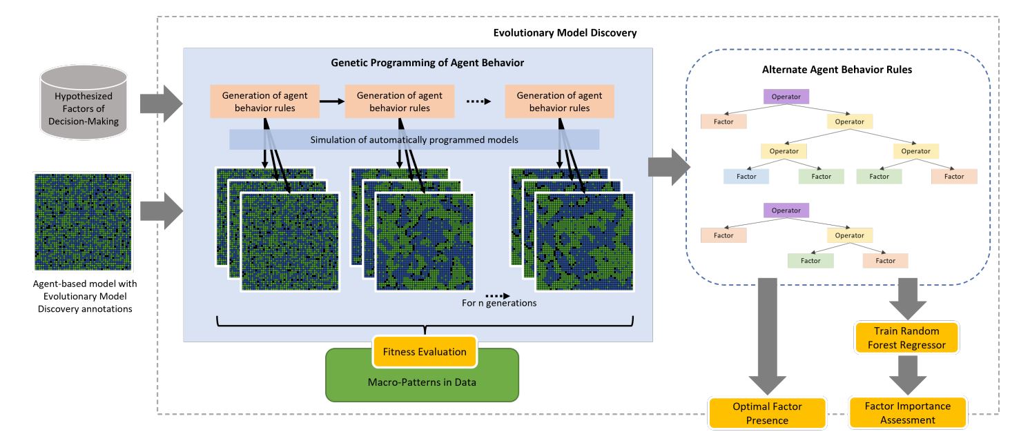
Evolutionary model discovery combines genetic programming and random forest importance analysis to identify the individual-level factors leading to the emergence of a target macro-phenomena (Gunaratne 2019; Gunaratne et al. 2021; Gunaratne & Garibay 2020). Evolutionary model discovery works in two stages as illustrated in Figure 1.

First, genetic programming is used to evolve the agent rule representing the individual-level behavior. For this, NetLogo implementations of factors hypothesized to influence the behavior must be provided along with a fitness function that evaluates the performance of each resulting simulation. The genetic program then creates generations of variants of the original model by combining factors with operators to produce different agent rules. These variants are then evaluated for their fitness to target phenomenon. The fittest rules are then selected for reproduction of the next generation. Crossover and mutation operators are applied on the selected parent rules to produce a new generation of child rules. This process is repeated for a number of generations, resulting in the gradual exploration of rules that help the agent-based model more accurately reproduce the target phenomenon. For each genetic program individual produced during this process, the factor presence to simulation fitness data is recorded.

Factor presence is estimated as the coefficient of the factor in the mathematically simplified version of the rule, and may be a negative of positive integer. If higher order operators such as multiplication and division are used, then new factors, i.e. interactions of the original factors, may be produced for which the factor presence will be measured separately. Several simulations of each model variant produced by a rule resulting from the genetic program are run in order to account for the stochasticity of the agent-based model. This way the genetic program produces a synthetic dataset of factor presence to simulation fitness. Genetic programming has been increasingly used successfully in several other studies to generate agent rules from atomic explainable factors for complex social systems (Ekblad & Herman 2021; Greig & Arranz 2021; Miranda 2022; Vu et al. 2019; Vu et al. 2021; Vu et al. 2022).

Second, the generated factor presence to simulation fitness dataset is used to train a random forest regressor. The trained random forest regressor is then made to predict the fitness of a holdout of this dataset, given factor presence values. Then, permutation importance is estimated for each factor (and factor interaction) on the random forest’s ability to predict the simulation fitness. Permutation importance of a selected input feature is measured by randomly permuting that feature, breaking its relationship to the output (Breiman 2001). The predictive score obtained by permuting the feature subtracted from the score of the original model is calculated as the permutation importance of that feature.¹ A feature of higher importance would cause the random forest to have much larger loss in score when permuted and result in a higher permutation importance. This way an approximation of the importance of the considered factors, and factor interactions, (features to the random forest) in generating the target phenomenon is obtained. The most important factors are thus identified along with their optimal marginal presence values at which simulation fitness is maximized.

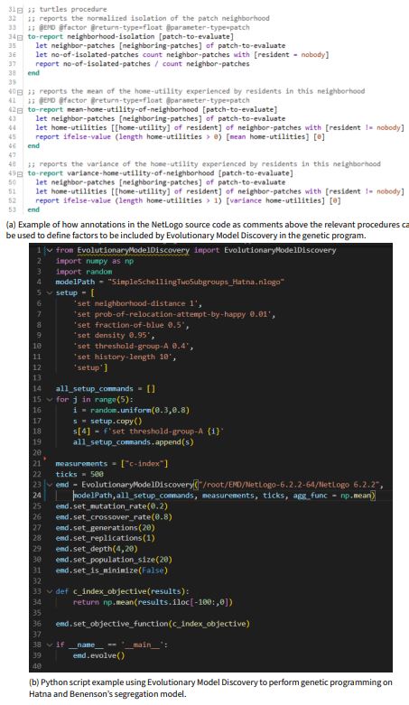
Evolutionary model discovery is implemented as an open-source Python package available on pypi.org. Evolutionary model discovery is able to pick up annotations from the NetLogo code to determine what NetLogo procedures represent factors and operators to be included in the the genetic program. The line of code in the NetLogo model to be evolved by the genetic program must also be annotated. Evolutionary model discovery can then be invoked on the NetLogo model through a Python script where the hyperparameters for the genetic program and the analysis via the random forest can be written. Figure 2 demonstrates how NetLogo annotations can be set up, while Figure 2 shows an excerpt from the Python script.

Experiments

We implemented Hatna and Benenson’s model (Hatna & Benenson 2015) in NetLogo and extended it to work with the Evolution Model Discovery². The calculation of residential satisfaction, \(u_{a,i}\), was tagged as the entry point for the Evolutionary Model Discovery with implementations of the factors as defined above. The code used for the experiments is made available at: https://github.com/chathika/modelsofsegregation.

The genetic program hyperparameters for evolutionary model discovery were set as follows. Mutation rate was set to \(0.2\), single-point crossover was used at a rate of \(0.8\), minimum rule depth was set to \(4\), maximum rule depth was set to \(20\), and population size was set to \(20\) models per generation over \(20\) generations. Each agent rule, represented by an individual of the genetic program, was automatically parsed into NetLogo code and each resulting model was replicated over \(5\) simulations. The mean C-index over the last \(100\) ticks was measured and reported for each simulation as its fitness. The mean fitness of the \(5\) simulation replicates of each individual of the genetic program was reported as the fitness of that individual. The results over \(5\) genetic program runs were used for factor importance analysis through random forest regression.

1 found that C-index is highest when equal proportions of the two races (blue and green) were present. Accordingly, for each simulation, the ratio of blue agents to green agents was set to \(0.5\). For each simulation, \(\hat{\theta}_{a}\) was randomly selected from the range \([0.3, 0.8]\) and set equal for all agents of both races. Density was set to \(D = 0.95\). The probability of a happy agent relocating, \(m\), was set to \(0.01\). Neighborhoods were considered as the grid locations \(1\) hop away from a patch. The model was run for \(500\) ticks per simulation.

Results

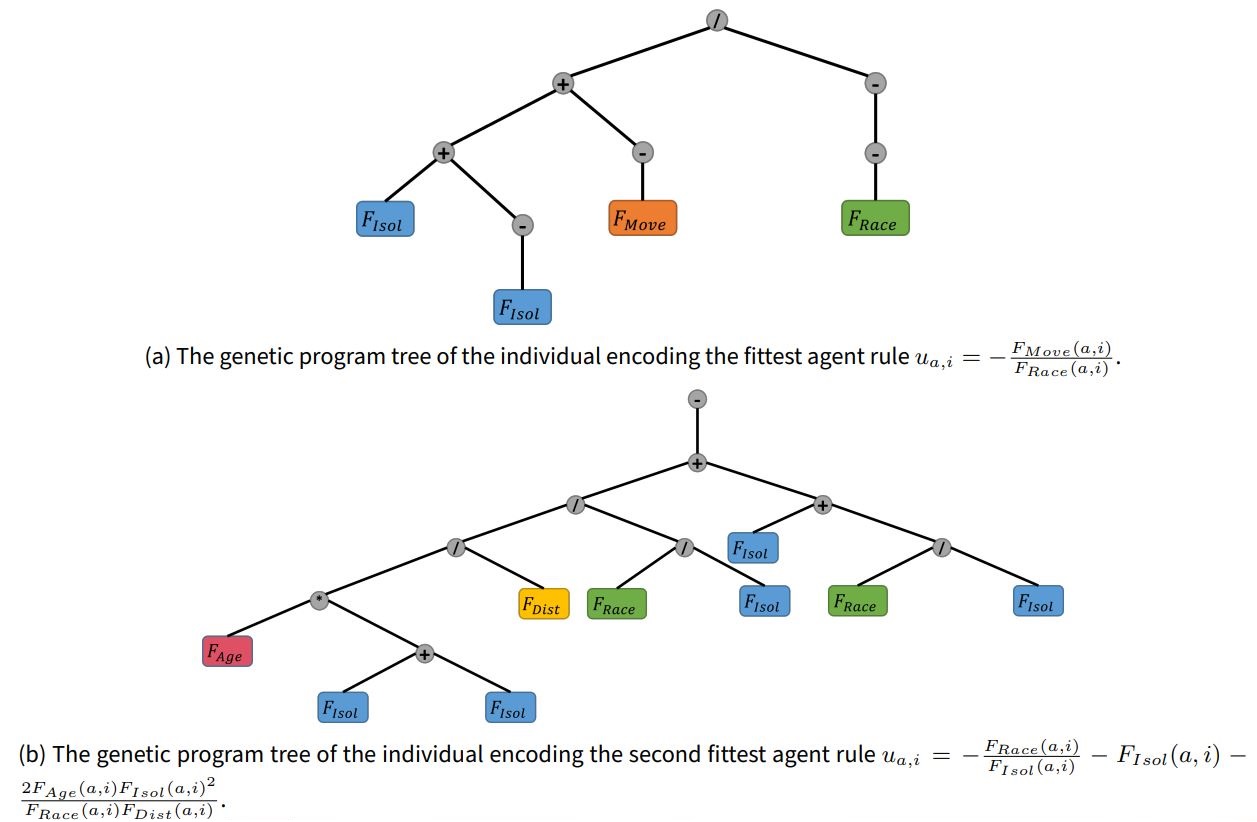
The genetic program produced rules of varying numbers of terms joined by \(+\) operators, negated by \(-\) operators, and factor interactions created by \(*\) and \(/\) operators. Some genetic program individuals resulted in deep trees, whose complexity could be reduced through mathematical simplification once decoded into equation form. Two examples of such trees along with their resulting simplified rules are shown in Figure 3 for the two best performing genetic program individuals.

It was seen in several instances that the \(+\) and \(-\) operators had been used as ‘padding’, increasing the tree size with no contribution to the encoded rule nor, in turn, to fitness, a phenomenon inherent to genetic programming as ‘bloat’ (Banzhaf & Langdon 2002; Langdon & Poli 1998; Luke & Panait 2006). Setting the maximum tree depth helped keep tree bloat within reasonable bounds. These inexpressive sections of the trees also acted as ‘introns’ (Luke 2000), i.e. reasonable positions for the crossover operations of the genetic program to introduce new expressive branches, without disrupting the fitness generated by the existing expressive branches of the tree.

For the rest of the results, we only considered rules that were generated at least 10 times by the genetic program, in order to have an adequate number of C-index samples for analysis.

Table 1 displays the simplified rules and mean C-index produced by the 10 highest fit individuals of the genetic program. The most fit rule, \(u_{a,i}=-\frac{F_{Move}(a,i)}{F_{Race}(a,i)}\), produced the highest mean C-index by far, \(0.3047\), a magnitude higher than that produced by the original Schelling rule \(u_{a,i}=F_{Race}(a,i)\) and near the theoretical maximum C-index. This was also higher than the maximum C-index seen by 1 when using \(u_{a,i}=F_{Race}(a,i)\) with heterogeneous parameters. The second best rule, \(u_{a,i}=-\frac{F_{Race}(a,i)}{F_{Isol}(a,i)} - F_{Isol}(a,i) - \frac{2F_{Age}(a,i)F_{Isol}(a,i)^2}{(F_{Race}(a,i)F_{Dist}(a,i))}\), produced less mean C-index than the first at 0.2260 and is considerable more complex, with three terms, four unique factors, and its simplified form even contained a squared term. The next 5 rules were similarly complex and with steadily decreasing mean C-index. Interestingly, the second best rule comprised of nearly all hypothesized factors other than \(F_{Move}(a,i)\). The 8^th, 9^th, and 10^th were considerably simpler, and included single factor rules, \(u_{a,i}=F_{Race}(a,i)\) and \(u_{a,i}=F_{Age}(a,i)\), with mean C-index 0.0607 and 0.0313, respectively. Also of note is that \(F_{Race}(a,i)\) is included in all of the top 9 rules.

Table 1: Simplified rules of best 10 genetic program individuals that produced the highest mean C-index, greatest mixing of segregated of integrated residential locations.

Rule	Mean c-Index
\(u_{a,i}=-\frac{F_{Move}(a,i)}{F_{Race}(a,i)}\)	\(0.3047\)
\(u_{a,i}=-\frac{F_{Race}(a,i)}{F_{Isol}(a,i)} - F_{Isol}(a,i) - 2\frac{F_{Age}(a,i)F_{Isol}(a,i)^2}{F_{Race}(a,i)F_{Dist}(a,i)}\)	\(0.2260\)
\(u_{a,i}=-\frac{F_{Race}(a,i)}{F_{Isol}(a,i)} - F_{Isol}(a,i) - \frac{F_{Age}(a,i)F_{Isol}(a,i)}{F_{Race}(a,i)} - \frac{F_{Age}(a,i)F_{Isol}(a,i)^2}{F_{Race}(a,i)F_{Dist}(a,i)}\)	\(0.1804\)
\(u_{a,i}=-\frac{F_{Race}(a,i)}{F_{Isol}(a,i)} - F_{Isol}(a,i) - \frac{F_{Age}(a,i)}{F_{Race}(a,i)} - \frac{F_{Age}(a,i)F_{Isol}(a,i)}{F_{Race}(a,i)F_{Dist}(a,i)}\)	\(0.1777\)
\(u_{a,i}=-\frac{F_{Race}(a,i)}{F_{Isol}(a,i)} + \frac{F_{Age}(a,i)}{F_{Isol}(a,i)} - F_{Isol}(a,i) + \frac{F_{Age}(a,i)}{F_{Dist}(a,i)}\)	\(0.1009\)
\(u_{a,i}=\frac{F_{Age}(a,i)^2}{F_{Race}(a,i)}\)	\(0.0790\)
\(u_{a,i}=-\frac{F_{Race}(a,i)}{F_{Isol}(a,i)} + \frac{F_{Age}(a,i)}{F_{Isol}(a,i)} + \frac{F_{Age}(a,i)}{F_{Dist}(a,i)}\)	\(0.0699\)
\(u_{a,i}=F_{Race}(a,i)\)	\(0.0607\)
\(u_{a,i}=\frac{F_{Race}(a,i)}{F_{Age}(a,i)}\)	\(0.0358\)
\(u_{a,i}=F_{Age}(a,i)\)	\(0.0313\)

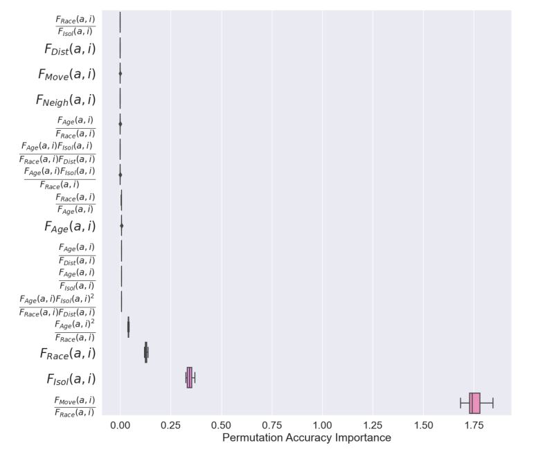
The results of random forest permutation importance analysis on the data produced by the genetic program are displayed in Figure 4. The results confirmed that the factor interaction \(\frac{F_{Move}(a,i)}{F_{Race}(a,i)}\) has by far the highest importance, approximately 1.75, more than 4 times as important as \(F_{Isol}(a,i)\), the second most important factor. In addition to these two factors, \(F_{Race}(a,i)\) and \(F_{Age}(a,i)^2/F_{Race}(a,i)\) had lower permutation importance and all other factors and factor interactions had relatively negligible importance in determining C-index.

Figure 5 displays the marginal distributions of C-index produced under varying presence of each of the four most important factors in the simplified rules (presence of \(0\) is not included as this indicates the factor is absent in the rule). Only presence values for which there were sufficient samples (at least 10) are shown, and for all four factors, this limited presence to either \(-1\) or \(1\). Rules with the factor of highest importance \(\frac{F_{Move}(a,i)}{F_{Race}(a,i)}\) had very high C-index, typically over \(0.3\) and near the theoretical maximum, at presence of \(-1\). There was no significant sample of this factor at presence of \(1\). Next, rules with the second most important factor \(F_{Isol}(a,i)\) had a wide range of C-index values from approximately \(0.08\) to as high as \(.25\) for presence of \(-1\). Near zero C-index was seen when presence was at \(1\). For rules with \(F_{Race}(a,i)\), several clusters of C-index were seen, each below \(0.15\) for presence \(1\) and no significant sample was seen at \(-1\). Finally, a cluster of rules with the factor \(F_{Age}(a,i)\) at presence \(1\) were observed with C-index typically between \(0.05\) and \(0.12\), while there was no significant sample for presence of \(-1\).

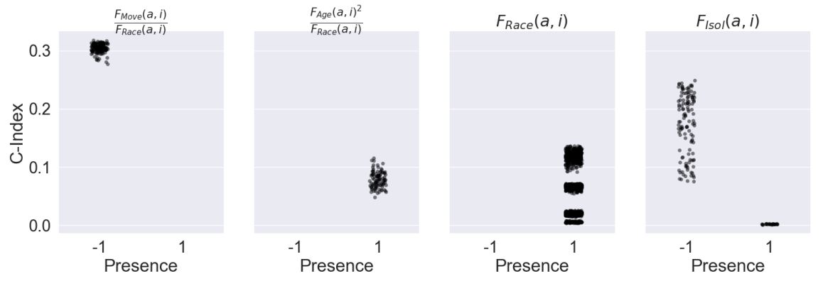
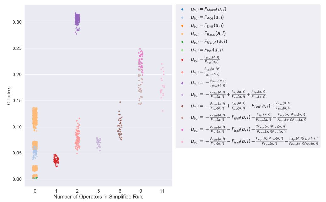
Figure 6 displays a stripplot of of the C-index of commonly generated rules by the number of operators in the simplified rule. The points in the plot are color coded by rule. The number of operators in the simplified rule was taken as a proxy of rule complexity. It can be seen that the there was a linear, positive trend between increasing number of operators and minimum C-index produced. However, despite this trend, at rule complexity of 2, the best performing rule \(u_{a,i}=-\frac{F_{Move}(a,i)}{F_{Race}(a,i)}\) exhibited an anomalously high C-index that is not representative of the rest of the rules. This demonstrated the deceptiveness of the underlying fitness landscape created by the problem at hand and the difficulty of deriving such a rule by hand without the automation of evolutionary search. Furthermore, it was seen that most rules had little or no operators, despite deep trees being generated by the genetic program, again demonstrating the effect of tree bloat.

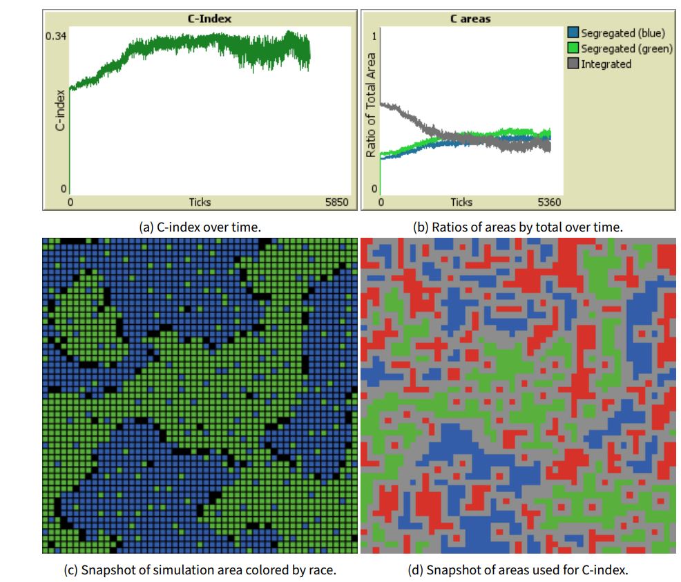
The progression of C-index over time for the best performing rule \(u_{a,i}=-\frac{F_{Move}(a,i)}{F_{Race}(a,i)}\), over 5,000 ticks at \(\hat{\theta}_a=0.48\) is shown in Figure 7 a. It can be seen there was a steady increase in C-index until around 1,800 simulation. C-index remained high throughout the rest of the simulation with some variation as fully satisfied agents still had a small probability of relocating (\(m= 0.01\)). Maximum C-index (\(\frac{1}{3}\)) was reached was reached around 4,590 ticks. Figure 7 b shows the ratios of the segregated areas for both races and the mixed area by total area, over time. C-index was maximized when these ratios were equivalent, as it is equal to the smallest of the three ratios. We can see that the segregated areas grew gradually and quite similarly, drawing agents from the mixed area which decreased steadily. All three ratios were approximately equal around 2300 ticks after which there wer slight variations, but generally remained quite similar to one another.

Figure 7 c shows a snapshot of the simulation area at peak C-index colored by race. Figure 7 d shows the same instance colored by area used for C-index calculation with the blue and green areas being labeled segregated, the red areas being labeled as mixed, and the grey areas ignored as boundaries. It can be seen that the solution produced smaller segregated and mixed areas, which was different from the large segregated patches produced by 1. The reason for this was that C-index does not consider the area size to perimeter ratio allowing for more diffused segregated and mixed patterns to score highly.

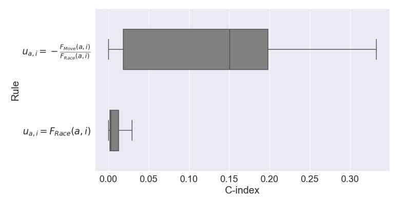
In order to test the robustness of the best performing rule, \(u_{a,i}=-\frac{F_{Move}(a,i)}{F_{Race}(a,i)}\), over the original Schelling rule, \(u_{a,i}=F_{Race}(a,i)\), the boxplot in Figure 8 shows the comparison between C-indices of 100 simulations of both models under \(\hat{\theta}_a\) being uniform randomly selected from the range \([0.3, 0.8]\). A large improvement in fitness was produced under \(u_{a,i}=-\frac{F_{Move}(a,i)}{F_{Race}(a,i)}\), and as the two boxes do not overlap, \(u_{a,i}=-\frac{F_{Move}(a,i)}{F_{Race}(a,i)}\) can be said to have had a significant improvement over the original Schelling rule. As this rule performed better despite the variation of \(\hat{\theta}_a\), we can conclude that it was also more robust to varying utility thresholds of the agents.

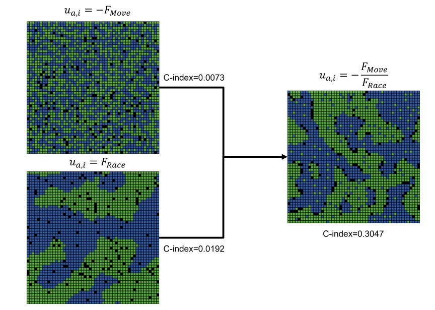
It is important to emphasize that neither of the two original factors of the best performing rule, \(F_{Move}(a,i)\) and \(F_{Race}(a,i)\) were able to produce mixed patterns independently. As shown in Figure 9, independently, \(u_{a,i}=-F_{Move}(a,i)\) produced highly integrated patterns, while \(u_{a,i}=F_{Race}(a,i)\) had a tendency to produce highly segregated patterns, as in Schelling’s original model, but not mixed patterns. However, the interaction of these two factors within the same rule, especially with the inversion of \(F_{Race}(a,i)\) via a division operator, led to the emergence of mixed patterns of segregation and integration.

Analyzing this rule further, we see that \(F_{Race}\) has a negative, nonlinear relationship with \(u_{a,i}\), with very low values of \(F_{Race}\) severally penalizing \(u_{a,i}\), but this effect quickly diminishes for moderate and higher values of \(F_{Race}\) to where there is very little difference. \(F_{Move}\) acts as an amplifier of this effect. Higher \(F_{Move}\) increases the range through which \(F_{Race}\) is more discriminatory. While lower \(F_{Move}\) drastically decreases any effect of \(F_{Race}\) to very low values. In other words, for agents with this rule, \(F_{Race}\) had a positive nonlinear, rapidly diminishing effect on \(u_{a,i}\), only severely discriminating at very low values, while \(F_{Move}\) amplified this relationship, making is stronger as it increased. These agents were typically less racially biased, yet exhibited strong desire to relocate if there was not at least one racially similar agent. This discriminatory effect was amplified as the agent relocated more, forcing such agents into more segregated areas, until they found sufficiently similar neighbors. After settling, and clearing their recent relocation history, these agents return to being less discriminatory.

Discussion

Evolutionary Model Discovery was applied to automate the discovery of factors causing the emergence of mixed patterns of coexisting residential segregation and integration. Hatna & Benenson (2012), 1 have shown that in reality, urban communities are neither completely segregated nor completely integrated, but have coexisting mixed patterns. Agents of Benenson and Hatna’s model of mixed patterns embody the same factor for evaluating the residential desirability offered by potential new locations for relocation as that originally posited by Schelling (1971). In these models, residential satisfaction is dependent solely on racial bias, i.e. neighborhoods with a sufficient number of neighbors of similar race. There are three respects in which our treatment differed from 1, when generating mixed patterns. First, in Benenson and Hatna agents are heterogenous in terms for their racial bias (i.e. agents vary in their tolerance for others), while in our study, they were homogenous in terms of parameters. Second, in Benenson and Hatna, only racial bias was considered, while here we considered several factors beyond racial bias. Third, Benenson and Hatna vary only the parameters, while in our study we evolved the agents’ behavior rule. Rule generation was automated using genetic programming and evaluated using random forests. The metric used to characterize mixed patterns was the C-index, introduced by Hatna & Benenson (2012).

Our results indicate that the coexistence of mixed patterns of segregation and integration was better explained when social factors, besides racial bias, were considered. Moreover, we demonstrate that strongly mixed patterns arose when individuals’ relocation decisions were governed by a nonlinear, rapidly diminishing preference for racial similarity amplified by historical tendency to move, as shown in the winning rule found by evolutionary model discovery, \(u_{a,i} = -\frac{F_{Move}(a,i)}{F_{Race}(a,i)}\). We interpret this rule as follows. \(-\frac{1}{F_{Race}}\) caused agents to remain satisfied with their neighborhoods unless there was a very low, or absent, number of neighbors of the same race. When this was multiplied by \(F_{Move}\), it amplified the discrimination of neighborhoods by those agents who did relocate, over those who did not, which in turn caused them relocate again, potentially triggering a positive feedback loop. This led to amplified mixing among a sub-population of agents who were unsatisfied (in addition to those who moved due to random noise), until these agents relocated to areas that did satisfy their increased racial bias, generating the more segregated areas. After these agents settled and their recent move history cleared, \(F_{Move}\) decreased, reducing their discriminatory nature and limiting future relocation. Those agents that did not relocate continued to be less discriminatory and formed the integrated areas. It is by this duality in behavior that mixed patterns are thus formed. This rule, had a mean C-index of \(0.3047\) across varying threshold parameter values and at times reached the theoretical maximum C-index of \(\frac{1}{3}\). It was therefore able to outperform the C-index of mixed patterns produced by 1, where the original Schelling rule based on linear racial bias was calibrated under heterogeneous parameters for a maximum C-index of approximately 0.2.

A much weaker, but competing theory that emerged from this work was that weaker mixed patterns (still with a C-index above 0.2) could also arise from a more complex combination of preference for racial diversity, aversion of isolated areas, and/or a preference for neighborhoods where residents have resided for a longer period of time and are closer to their current residence, as can be seen in the 2^nd to 4^th best rules.

The patterns that were generated by the best rule differed somewhat from those obtained in 1, where larger and fewer regions of integration and segregation were observed. In contrast, the best performing rule in this study produced many smaller areas of integration and segregation to produce a higher C-index. This is due to the fact that C-index does not consider the area to boundary ratio ratio of the segregated and integrated areas in its calculation. It is therefore unable to distinguish between these two cases. C-index was the sole objective of the genetic program in this study, so evolutionary model discovery may have generated either pattern, however we did not visualize the patterns generated by each rule. The results of this study reveal that a different metric would be required if the size and number of segregated and integrated areas were to be optimized and potentially also require multi-objective genetic programming. This paves the way for future work for multi-objective inverse generative social science.

Conclusion

This modeling exercise illustrates several core features of iGSS (inverse Generative Social Science) discussed by Epstein (2023). First, rather than handcrafting the agents’ rules, we started with the macro target–mixed, not segregated, populations–and from a few factors and operators, we evolved micro-rules generating the target from the bottom up. In fact, the evolutionary model discovery framework evolved multiple such generators. The winner, though arrestingly simple (\(u_{a,i} = -\frac{F_{Move}(a,i)}{F_{Race}(a,i)}\)) includes two components that contributes to the generation of mixed patterns. The expression \(-\frac{1}{F_{Race}(a,i)}\) represents agents that are highly appreciative of an increase in the local proportion of their own group when it is a small minority, but less so as the proportion increases. This produces a nonlinear relationship exhibiting diminishing marginal returns to location utility with increasing neighborhood racial similarity. The multiplication by \(F_{Move}(a,i)\) represents the recent frequency of relocation and thus amplifies the agent’s discrimination of neighborhoods by race, encouraging relocation of any dissatisfied agents into more segregated areas and leaving those who are satisfied in integrated ones. One might expect to see \(F_{Dist}(a,i)\) as a surrogate for the amplification of mixing, but it is absent from the winning rule. Furthermore, the winning rule is highly fit. The theoretical maximum of the c-index being \(1/3\), the winner’s fitness (calibration to the target) of \(0.3047\) is impressive. The second place rule (also quite fit) is a much more complex and highly nonlinear expression that certainly did not occur to any of the authors. Not surprisingly, Schelling’s original rule does poorly. But as discussed in Epstein (2023), the iGSS approach retains it in a striking way. In Schelling’s rule generating strong segregation, racial preference (\(F_{Race}\)) is the only term and is the numerator. In evolving rules generating weak segregation (that is, mixed residential patterns), the iGSS approach retains racial preference but now as the denominator. As such, \(F_{Race}\) has a diminishing marginal effect on utility, again unlike the original. Particularly noteworthy is the elegance, simplicity, and interpretabilty of the winning rule.

While many extensions and refinements await, the present exercise demonstrates the power of the evolutionary inverse generative approach on a problem of enduring theoretical interest and pressing social importance.

References

BANZHAF, W., & Langdon, W. B. (2002). Some considerations on the reason for bloat. Genetic Programming and Evolvable Machines, 3(1), 81–91. [doi:10.1023/a:1014548204452]

BENENSON, I., & Hatna, E. (2011). Minority-majority relations in the Schelling model of residential dynamics. Geographical Analysis, 43(3), 287–305. [doi:10.1111/j.1538-4632.2011.00820.x]

BISWAS, B., Ahsan, M. N., & Mallick, B. (2021). Analysis of residential satisfaction: An empirical evidence from neighbouring communities of rohingya camps in cox’s bazar, bangladesh. Plos One, 16(4), e0250838. [doi:10.1371/journal.pone.0250838]

BISWAS, B., Sultana, Z., Priovashini, C., Ahsan, M. N., & Mallick, B. (2021). The emergence of residential satisfaction studies in social research: A bibliometric analysis. Habitat International, 109, 102336. [doi:10.1016/j.habitatint.2021.102336]

BLANCO, B. A., Poulson, M., Kenzik, K. M., McAneny, D. B., Tseng, J. F., & Sachs, T. E. (2021). The impact of residential segregation on pancreatic cancer diagnosis, treatment, and mortality. Annals of Surgical Oncology, 28, 3147–3155. [doi:10.1245/s10434-020-09218-7]

BREIMAN, L. (2001). Random forests. Machine Learning, 45, 5–32.

CLARK, W. A. (1986). Residential segregation in American cities: A review and interpretation. Population Research and Policy Review, 5, 95–127. [doi:10.1007/bf00137176]

EKBLAD, L., & Herman, J. D. (2021). Toward data-driven generation and evaluation of model structure for integrated representations of human behavior in water resources systems. Water Resources Research, 57(2), e2020WR028148. [doi:10.1029/2020wr028148]

EPSTEIN, J. M. (2023). Inverse generative social science: Backward to the future. Journal of Artificial Societies and Social Simulation, 26(2), 9. [doi:10.18564/jasss.5083]

FLIPPEN, C. A. (2001). Residential segregation and minority home ownership. Social Science Research, 30(3), 337–362. [doi:10.1006/ssre.2001.0701]

GREIG, R., & Arranz, J. (2021). Generating Agent Based Models From Scratch With Genetic Programming. [doi:10.1162/isal_a_00383]

GUNARATNE, C. (2019). Evolutionary Model Discovery: Automating causal inference for generative models of human social behavior. PhD Thesis, University of Central Florida

GUNARATNE, C., & Garibay, I. (2020). Evolutionary model discovery of causal factors behind the socio-agricultural behavior of the Ancestral Pueblo. PLoS ONE, 15(12), e0239922. [doi:10.1371/journal.pone.0239922]

GUNARATNE, C., Rand, W., & Garibay, I. (2021). Inferring mechanisms of response prioritization on social media under information overload. Scientific Reports, 11(1), 1–12. [doi:10.1038/s41598-020-79897-5]

HATNA, E., & Benenson, I. (2012). The schelling model of ethnic residential dynamics: Beyond the integrated-segregated dichotomy of patterns. Journal of Artificial Societies and Social Simulation, 15(1), 6. [doi:10.18564/jasss.1873]

HATNA, E., & Benenson, I. (2015). Combining segregation and integration: Schelling model dynamics for heterogeneous population. Journal of Artificial Societies and Social Simulation, 18(4), 15. [doi:10.18564/jasss.2824]

HERBST, C. M., & Lucio, J. (2016). Happy in the hood? The impact of residential segregation on self-reported happiness. Journal of Regional Science, 56(3), 494–521. [doi:10.1111/jors.12263]

LANGDON, W. B., & Poli, R. (1998). Fitness causes bloat: Mutation. European Conference on Genetic Programming [doi:10.1007/bfb0055926]

LEONARD, J. S. (1987). The interaction of residential segregation and employment discrimination. Journal of Urban Economics, 21(3), 323–346. [doi:10.1016/0094-1190(87)90006-4]

LUKE, S. (2000). Code growth is not caused by introns. Late Breaking Papers at the 2000 Genetic and Evolutionary Computation Conference, Las Vegas, Nevada, USA

LUKE, S., & Panait, L. (2006). A comparison of bloat control methods for genetic programming. Evolutionary Computation, 14(3), 309–344. [doi:10.1162/evco.2006.14.3.309]

MASSEY, D. S. (2015). The legacy of the 1968 fair housing act. Sociological Forum, 30(51), 571–588. [doi:10.1111/socf.12178]

MIRANDA, L. (2022). Humans in algorithms, algorithms in humans: Understanding cooperation and creating social AI with causal generative models. PhD Thesis, University of Central Florida

POULSON, M., Cornell, E., Madiedo, A., Kenzik, K., Allee, L., Dechert, T., & Hall, J. (2021). The impact of racial residential segregation on colorectal cancer outcomes and treatment. Annals of Surgery, 273(6), 1023–1030. [doi:10.1097/sla.0000000000004653]

SCHELLING, T. C. (1969). Models of segregation. The American Economic Review, 59(2), 488–493.

SCHELLING, T. C. (1971). Dynamic models of segregation. Journal of Mathematical Sociology, 1(2), 143–186.

VU, T. M., Buckley, C., Bai, H., Nielsen, A., Probst, C., Brennan, A., Shuper, P., Strong, M., & Purshouse, R. C. (2020). Multiobjective genetic programming can improve the explanatory capabilities of mechanism-based models of social systems. Complexity, 2020. [doi:10.1155/2020/8923197]

VU, T. M., Buckley, C., Duro, J. A., & Purshouse, R. C. (2022). Exploring social theory integration in agent-based modelling using multi-objective grammatical evolution. ICML 2022 Workshop AI for Agent-Based Modelling

VU, T. M., Davies, E., Buckley, C., Brennan, A., & Purshouse, R. C. (2021). Using multi-objective grammar-based genetic programming to integrate multiple social theories in agent-based modeling. International Conference on Evolutionary Multi-Criterion Optimization [doi:10.1007/978-3-030-72062-9_57]

VU, T. M., Probst, C., Epstein, J. M., Brennan, A., Strong, M., & Purshouse, R. C. (2019). Toward inverse generative social science using multi-objective genetic programming. Proceedings of the Genetic and Evolutionary Computation Conference [doi:10.1145/3321707.3321840]

VU, T. M., Probst, C., Nielsen, A., Bai, H., Buckley, C., Meier, P. S., Strong, M., Brennan, A., & Purshouse, R. C. (2020). A software architecture for mechanism-based social systems modelling in agent-based simulation models. Journal of Artificial Societies and Social Simulation, 23(3), 1. [doi:10.18564/jasss.4282]

YU, C.-Y., Woo, A., Hawkins, C., & Iman, S. (2018). The impacts of residential segregation on obesity. Journal of Physical Activity and Health, 15(11), 834–839. [doi:10.1123/jpah.2017-0352]