Bounded Confidence Revisited: What We Overlooked, Underestimated, and Got Wrong

Frankfurt School of Finance & Management, Germany
Journal of Artificial
Societies and Social Simulation 26 (4) 11
<https://www.jasss.org/26/4/11.html>
DOI: 10.18564/jasss.5257
Received: 11-Sep-2023 Accepted: 11-Sep-2023 Published: 31-Oct-2023
Abstract
In the bounded confidence model (BC-model) (Hegselmann and Krause 2002), period by period, each agent averages over all opinions that are no further away from their actual opinion than a given distance ε, i.e., their ‘bound of confidence’. With the benefit of hindsight, it is clear that we completely overlooked a crucial feature of our model back in 2002. That is for increasing values of ε, our analysis suggested smooth transitions in model behaviour. However, the transitions are in fact wild, chaotic and non-monotonic—as described by Lorenz (2006). The most dramatic example of these effects is a consensus that breaks down for larger values of ε. The core of this article is a fundamentally new approach to the analysis of the BC-model. This new approach makes the non-monotonicities unmissable. To understand this approach, we start with the question: how many different BC processes can we initiate with any given start distribution? The answer to this question is almost certainly for all possible start distributions and certainly in all cases analysed here, it is always a finite number of ε-values that make a difference for the processes we start. Moreover, there is an algorithm that finds, for any start distribution, the complete list of ε-values that make a difference. Using this list, we can then go directly through all the possible BC-processes given the start distribution. We can therefore check them for non-monotonicity of any kind, and will be able to find them all. This good news comes however with bad news. That is the algorithm that inevitably and without exception finds all the ϵ-values that matter requires exact arithmetics, without any rounding and without even the slightest rounding error. As a consequence, we have to abandon the usual floating-point arithmetic used in today’s computers and programming languages. What we need to use instead is absolutely exact fractional arithmetic with integers of arbitrary length. This numerical approach is feasible on all modern computers. The new analytical approach and results are likely to have implications for many applications of the BC-model.Introduction
Alfred Jules Ayer’s final remark 1978
in the BBC-Television series Men of Ideas.
Ayer was interviewed by Brian Magee;
cf. Magee (1982, 109).
The very essence of what now is known as the bounded confidence model (BC-model, for short) is simple: Period by period, all agents average over all opinions that are not further away from their actual opinion than a given distance \(\epsilon\), their ‘bound of confidence’. The model was described for the first time in Krause (1997 p. 47ff.), an article published in German. To refer to the model, the term bounded confidence was used for the first time by Krause in 1998, namely in a conference presentation in Warzaw, published as (Krause 2000 cf. 231). A first comprehensive analytical and computational analysis of the BC-model was given more than two decades ago in Hegselmann & Krause (2002).1 The model has a very close relative, namely the model in Deffuant et al. (2000). The main difference regards the updating procedure: In Hegselmann & Krause (2002) the updating happens simultaneously while Deffuant et al. (2000) use a pairwise sequential procedure.2 Soon it became a common practice to refer to both models as BC-models and to distinguish two variants: the Hegselmann-Krause model (HK-model for short) and the Deffuant-Weisbuch model (DW-model for short).
In terms of its definition, the BC-model is easy to understand—and it ‘invites’ all sorts of objections. But it is often easy to modify the model so that it covers the objection. This combination of features has made the model a kind of platform from which new projects can be started. And this probably explains, at least in part, why the model is highly cited (and still increasingly so). It is now even difficult to keep track of the survey articles in which the BC-model, its extensions, modifications or newly discovered analytical features are an important component.3
In the following, I will focus exclusively on the basics of the BC-model and our analysis of it back then in Hegselmann & Krause (2002). The retrospective diagnosis is: We completely overlooked a crucial feature of our model. For increasing values of the confidence level \(\epsilon\), our analysis at the time suggests smooth transitions in the model’s behaviour. But in fact the transitions are wild, chaotic and non-monotonic. For example, we thought that for increasing values of \(\epsilon\), the number of opinion clusters surviving after stabilisation would decrease monotonically. But this is wrong—it may well be the case that a larger \(\epsilon\) leads to more final clusters. The most dramatic example of such an effect is a consensus that falls apart for larger values of \(\epsilon\) (remember: the initial distribution is held constant). What is more, for increasing values of \(\epsilon\) such effects can occur many times.
Similarly, it is wrong to think that for a constant start distribution of opinions the width of the final stable opinion profile decreases monotonically as \(\epsilon\) increases. Again, for one and the same start distribution an increasing final profile width can occur many times. In Hegselmann & Krause (2002) we did not explicitly state what turned out to be wrong. But we did not write it down just because we thought it was obvious—the false belief was suggested in a very natural way by the way we were analysing at the time. Later in this article it will become clear how this could happen, and some lessons will become clear that can be taken away.
Jan Lorenz was the first to discover the wild, chaotic, and non-monotonic transitions. In his equally ingenious and insightful article Consensus Strikes Back in the Hegselmann-Krause Model of Continuous Opinion Dynamics Under Bounded Confidence (Lorenz 2006), he mentions and demonstrates all the non-monotonicities that I mentioned above. The title of his article hints at perhaps the most dramatic effect of this kind.4 My article focuses on all the non-monotonicities in BC-processes that Lorenz discovered. And in a sense, I also want to cover those that are still waiting to be discovered. To this end, I present a new and rather fundamental approach to the analysis of the BC-model. In the new approach, the non-monotonicities that we overlooked at the time become directly obvious; in a sense, they are even unmissable.
The new approach starts from the following simple, but fundamental question: Given a certain start distribution of opinions, where all opinions are real-valued numbers from the interval \([0,1]\), we can run the BC-dynamics for that start distribution with any of all the possible confidence levels \(\epsilon \in [0,1]\). This set of possible \(\epsilon\)-values is an uncountable infinity. Given all this, when we ‘play around’ with possible confidence levels, how many different BC-processes can we initiate with the given start distribution? The answer to the question is: Almost certainly for all possible start distributions, and certainly in all cases analysed below, it is always a finite number of \(\epsilon\)-values that make a difference for the processes that we start. Moreover, there is an algorithm that finds for any start distributions the complete list of \(\epsilon\)-values that make a difference. Such a list is invaluable. With it, we can directly go through all BC-processes that are possible given the start distribution. We can check them for non-monotonicities of any kind—and we will find them all.
This is obviously very good news. But it comes with some bad news: The algorithm that, inevitably and without exception, finds all \(\epsilon\)-values that matter, requires absolutly exact arithmetic without any rounding anywhere and without even the very slightest rounding error. As a consequence, we have to abandon the usual floating-point arithmetic as it is normally used in today’s computers and programming languages. What we have to use instead is an absolutely exact fractional arithmetic with integers of arbitrary length. This numerical approach is feasible on all modern computers (details later). But it comes at a high cost in terms of speed.
In what follows, I have put together a number of arguments that may seem unrelated at first. However, later on they merge into a common thread. The next section deals with the basics of BC-processes. I introduce some notational conventions and definitions. We will go through some application contexts and reflect on their status. I then describe the kind of dual visualisation of BC-processes that is used throughout the article. It is dual in the sense that it shows BC-processes simultaneously as a dynamical system with its trajectories evolving over time, and as a dynamical network with links emerging or disappearing over time. The new type of visualisation is a significant improvement on the old one in Hegselmann & Krause (2002), which did not show network structures.
Section 3 deals with the worst enemy of the BC-model. It is an enemy within, namely the ordinary floating-point arithmetic. I am afraid that no model is more susceptible to errors inherent in floating-point arithmetic than the BC-model. In the computation of BC-processes, it can easily happen that representational or operational floating-point errors (their order of magnitude is \(10^{-17}\)) cause subsequent errors of 16 orders of magnitude higher in the next period. We discuss four strategies for dealing with these numerical difficulties.
Section 4 introduces a concept that is key for our new type of analysis of BC-processes, namely \(\epsilon\)-switches (often called switches for short). They turn out to be the \(\epsilon\)-values that make a difference for BC-processes with a given constant start distribution. We apply the concept to an example and describe the algorithm that finds all \(\epsilon\)-switches for any start distribution. Based upon the discussion in Section 3, it is clear that the algorithm requires absolute numerical accuracy which floating-point arithmetic is inherently incapable of providing. There is no other choice but to abandon the usual floating-point arithmetic and to resort to an absolutely exact fractional arithmetic throughout.
To gain more general insights about switches beyond our simple example, we apply the search algorithm to a larger class of start distributions, each with \(n\) opinions equidistantly spaced in the unit interval \([0,1]\). Since we know all of their \(\epsilon\)-switches from the algorithmic search, we look at their total number, and then focus on non-monotonicities, in particiular consents that fall apart again under the next larger \(\epsilon\)-switch.
In Section 5 we introduce a new graphical research tool, namely \(\epsilon\)-switch diagrams. Since we know all the \(\epsilon\)-values that make a difference, we can focus on these and only these values (i.e., the \(\epsilon\)-switches) and directly visualise the final cluster structure they produce. Such \(\epsilon\)-switch diagrams make it (well, almost) impossible to miss anything that we missed back in Hegselmann & Krause (2002).
In the final Section 6 we draw together some of the strands of argument and insights that have emerged along the way (some of them incidentally and by the way).
There are three appendices to this article. The purpose of these appendices is to keep the main text, which is already very long, free of very technical and advanced details that are not essential for understanding the central line of argument. The core of Appendix A is a series of numbered Analytical Notes which, stated in a more formal and technical language, consider central properties of \(\epsilon\)-switches in general. Appendix B focuses both on universal properties of equidistant start distributions, presented as Analytical Notes as in Appendix A, and on figures showing additional universal properties not covered by the figures in the main text. Many properties of floating-point arithmetic play an important role in this article. I have included only the most important in the main body of the article. When working with the BC-model, modifying and extending it, one needs to know more. Therefore, there is an Appendix C which, in my opinion, contains the minimum of what (at least, but better not only) BC-modelers should know about floating-point arithmetic.
BC-Processes: Definition, Application, Visualisation
Notation and definitions
In a first step we introduce some terminology that finally will allow us to state precisely what we mean by a BC-process (or, equivalently, BC-dynamics):
- There is a set \(I\) of \(n\) agents; \(i, j = 1, \dots, n\); \(i, j \in I\).
- Time is discrete; \(t = 0, 1, 2, \dots\).
- Each individual starts at \(t=0\) with a certain opinion, given by a real number from the unit interval; \(x_{i}(0) \in [0,1]\).
- The profile of opinions at time \(t\) is
\[X(t)= x_{1}(t), \dots , x_{i}(t), \dots, x_{j}(t), \dots, x_{n}(t).\] \[(1)\] - Each agent \(i\) takes into account agents \(j\) whose opinions are not too far away, i.e., for which \(|x_{i}(t) - x_{j}(t)| \leq \epsilon\), where \(\epsilon\) is the confidence level.5 That level determines the size of \(i\)’s confidence interval \([x_{i}-\epsilon, x_{i} + \epsilon]\).6
- The set of all agents \(j\) that \(i\) ‘takes seriously’ at time \(t\) (and given \(\epsilon\)) is:
i.e., the set of all agents in \(i\)’s confidence interval. For short, we will often refer to \(I\bigl(i,X(t), \epsilon \bigr)\) as the set of \(i\)’s \(\epsilon\)-insiders. Correspondingly, the set of \(i\)’s \(\epsilon\)-outsiders is the complimentary set of \(I\bigl(i,X(t), \epsilon \bigr)\), namely\[ I\bigl(i,X(t), \epsilon \bigr)= \{j\big||x_{i}(t) - x_{j}(t)| \leq \epsilon \},\] \[(2)\] \[ O\bigl(i,X(t), \epsilon \bigr) = I\bigl(i,X(t), \epsilon \bigr)^C = \{j\big||x_{i}(t) - x_{j}(t)| > \epsilon \}.\] \[(3)\] - The updated opinion of agent \(i\) is the arithmetic mean of all opinions \(x_{j}(t)\) for which \(j \in I\bigl(i,X(t), \epsilon \bigr)\):
\[ x_{i}(t+1)= \frac{1} {\lvert I\big( i,X(t), \epsilon \big)\rvert} \sum_{j \in I\bigl(i,X(t),\epsilon \bigr)} x_{j}(t).\] \[(4)\]
Based upon (1)-(7), we can now define: A sequence of opinion profiles is a BC-process if and only if it is generated by the updating rule (Equation 4). Obviously, a BC-process is uniquely characterised by the start distribution \(X(0)\) together with a confidence level \(\epsilon\). Therefore, in the following we will often refer to a BC-process simply by the ordered pair \(\langle X(0),\epsilon \rangle\).7 Formally, the process is an \(n\)-dimensional dynamical system.
Some second-order reflection upon the syntactical and semantical status of (1)-(7) helps to avoid major confusions and misunderstandings: The very heart of the characterisation of BC-processes is given in Equation 4. The preceding introduction of the set \(I\), the discrete time \(t\) etc., that is all the preparatory provision of terms that are used in Equation 4. As such, Equation 4 is a mathematical formalism only. However, by a preceding sentence like “There is a set \(I\) of \(n\) agents; \(i, j \in I.\)”, we give the formalism an interpretation that, if only in a sketchy way, hints at an intended type of applications—an application on what we normally call ‘agents’. Another provision says that the components of a profile \(X(t)\) should be understood as opinions. Additionally, a time sequence is assumed. As a consequence, we can read Equation 4 as an exactly specified interaction process of agents and their opinions over time.8
Altogether, we thus obtain by (1)-(7) all that we need for a syntactically and semantically sufficiently clear definition of the predicate “... is a BC-process”. This definition explicitly introduces a new predicate. Whoever understands a predicate, understands a concept as the meaning of that predicate—and that is something that is the same in all the concrete, written or spoken occurrences of the predicate somewhere in time and space, including occurrences as a synonymous term in different languages. But, then, what is exactly meant by the term “BC-model”? Throughout this article, I use the expression “BC-model” as a (meta-language) name for the (object-language) predicate “... is a BC-process”.
One should also be clear that predicates (as well as the concepts that constitute their meaning), are not the kind of entities that can be said to be true or false—and that holds for a primitive predicate like “... is green” as well as for our less primitive predicate “... is a BC-process”. Empirical truth or empirical falsity comes into play by a claim that a particular real-world process is an instance of a predicate (or falls under the concept that constitutes the meaning of this predicate). Such assertion sentences express propositions, and only they, the propositions, are capable of being true or false. Given the definition and the whole mathematical apparatus logically connected with it, logical-mathematical propositions can also be formulated and possibly proved. However, these are logical-mathematical truths, not empirical truths.
Some application contexts
As far as the types of representable opinions are concerned, the BC-model is more general than one might think at first: It could be about the putative probabilities, which themselves may concern qualitative, comparative, or quantitative issues. The opinions may concern any real-valued quantitative problem, provided that one can reasonably normalize the range of possible opinions to the unit interval. The opinions could concern, for example, the length of a river or the lifetime of a car. Opinions could express the intensity or importance of a desire.9 They could be opinions about moral desirability (0: extremely bad; 0.5: neutral; 1: extremely good). Or the opinions could concern a desirable budget share. On the other hand, non-continuous opinions, e.g., discretized or binary opinions, are not covered.
Apart from the different types of opinions, there are quite different contexts of possible applications. Here some (not mutually exclusive) examples:
- Compromise contexts: There is a group of people that exchange their views. For reasons such as uncertainty, interest in compromise, a preference for conformity, or even some social pressure, everyone is willing to move into the direction of the others’ opinions. However, there are limits to the willingness to compromise: An individual \(i\) with view \(x_i(t)\) is willing to compromise with individuals with opinions that are not too far away—and over them is averaged.
- Social media contexts: There is a digital platform with a central algorithmic coordination that matches user \(i\) with users \(j\) whose opinions \(x_j(t)\) are not too far away from \(i\)’s opinion \(x_i(t)\). User \(i\) then averages over these opinions. In such a context, \(\epsilon\) is the distance tolerance of a centrally organized filter bubble. Another social media variant would be a digital platform that allows all users \(j\) to send their opinions \(x_j(t)\) to all other users \(i\). As a recipient, however, user \(i\) only takes note of opinions that are not too far removed from his or her opinion. The average is then formed over these values. In this variant, \(\epsilon\) is the distance tolerance of a decentralised echo chamber.10
- Expert-disagreement contexts: There is a group of experts on something. Each expert has a well-considered opinion about the problem in question. Nevertheless, they disagree. And then what? In social epistemology, a much-discussed resolution proposal is “Split the difference!” (Douven & Riegler 2010 cf. 148). But what does that mean, and where does it lead to? The BC-model can be seen as a formal specification of the conflict resolution advise. In that perspective, the BC-model becomes a tool to answer normative or technical questions in the now blossoming field of (computational) social epistemology: The qualitative advise “Split the difference!” becomes a quantitative advise with regard to bounds of confidence, i.e., \(\epsilon\)-values. Their very different effects can be precisely computed and, then, evaluated from the point of view of their epistemic desirability.
With regard to the first two contexts, the BC-model could be seen as a direct idealising definition of a mechanism that is likely to play a greater role in these contexts. The mechanism could explain how, under certain conditions, effects often described or explained by terms such as homophily, conformity or confirmation bias occur.
Another way of looking at the BC-model would be to see the model itself as a more precise, specified, and metric re-definition of what is addressed by broad and qualitative concepts such as homophily, confirmation or conformity bias, which themselves summarily ‘conceptualize’ findings from countless empirical studies. The re-definition is tailored to dynamical contexts, continuous opinions as the subject matter, and circumstances in which homophily, confirmation or conformity effects come in degrees and with limits. What we do is a kind of conceptual engineering and very similar to what Rudolf Carnap (1891–1990) called an explication.11 He describes the procedure in chapter one of his Logical Foundations of Probability (Carnap 1950 pp. 1–18).12 In Carnap’s view, an explication transforms a more or less ambiguous, prescientific concept, the explicandum, into an improved concept, the explicatum. Carnap formulates four adequacy conditions:
A concept must fulfill the following requirements in order to be an adequate explicatum for a given explicandum: (1) similarity to the explicandum, (2) exactness, (3) fruitfulness, (4) simplicity (1950 p. 5).
In Carnap’s case, the prescientific terms are ‘confirming evidence’, ‘degree of confirmation’ or ‘probability’; cf. (1950 p. 21). His explicatum is the precise concept ‘degree of confirmation’. We can look at ‘homophily’, ‘confirmation bias’ or ‘conformity bias’ as explicanda, and consider the definition of BC-processes as their explicatum. Carnap’s four adequacy conditions are relevant in our case as well. But then there may be a difference: Carnap calls the explicandum a prescientific concept (cf. 1950 p. 1 et passim). With regard to my explicanda, I do not want to talk like that. Rather, it is simply that the very broad and qualitative concepts of homophily, confirmation or conformity bias are specified, made more precise, and quantified through their explication. The explicandum gets transformed, but not with the intention to replace it in all contexts.
Obviously, the broad and qualitative concepts of homophily, confirmation or conformity bias can be explicated in other ways than through the BC-model. One could think of non-real-valued opinions, continuous time or non-simultaneous updating. Thus, even as a mere explication of ‘homophily’, ‘confirmation bias’ or ‘conformity bias’, the-BC model does not have any claim to exclusivity.
In terms of content, the BC-model describes a mechanism: certain parts, namely agents with certain opinions, interact in a precisely defined way and thereby cause certain phenomena to occur. In opinion formation processes, however, there are also plausible mechanisms of a quite different kind, for example those in which the distance \(|x_i - x_j|\) is irrelevant. Each agent \(i\) could assign a weight \(w_{ij}\) to each other agent \(j\) and also to himself, which expresses the power, authority, competence et cetera assumed by \(i\) in \(j\). Let the sum of the weights that \(i\) assigns always be \(1\), and let the assignment of weights be constant over time. The updating is then done as a weighted averaging:
| \[ x_{i}(t+1)= \sum_{j \in I} w_{ij} \cdot x_{j}(t) \text{ with } 0 \leq w_{ij} \leq 1 \text{ and } \sum_{j \in I} w_{ij}= 1 .\] | \[(5)\] |
The mechanism characterised in this way can be traced back to French Jr (1956), Harary (1959) and DeGroot (1974). Today it is often referred to as the DeGroot model. I will do the same and refer to it as the DG-model or DG-processes. There are other mechanisms that can lead to a repulsive drifting apart of opinions.
In real-world opinion-formation processes of groups or even entire societies, a multitude of different mechanisms are likely to be at play, both individually and collectively. This does not bode well for realistic agent-based models. Precisely this could be a reason to rely on a completely different kind of modelling, namely machine learning based on gigantic data sets (big data). Technically, however, the modelling is then only implicit, i.e., hidden in a neural network, and thus largely opaque to humans; in any case, massive problems arise with regard to transparency, interpretability and explainability of what the model actually does.13 However, even without explicit human understanding of such a model, it might still be possible to make extremely good predictions with the model. This creates an entirely new epistemic situation which, together with other breakthroughs in AI that are equally disruptive to the intellectual position of the homo sapiens, requires a fundamental rethinking and redefinition of desirable epistemic ideals for beings like us.
Be that as it may, the BC-model is in any case epistemically old-fashioned: it aims at explicit understanding14,is deliberately kept simple, and precisely defines a certain mechanism, which is then examined in isolation and with conscious disregard of all other influences.15 It is clear from the outset that countless other mechanisms may be at play in actual opinion formation processes. With regard to what can be achieved with the model in descriptive terms, epistemic modesty is called for: The BC-model tells us something about what happens in a context in which it describes the predominant mechanism. Depending on the accuracy with which one knows the initial conditions in such a context, one can then describe, explain or predict accordingly. However, all of this is only possible under the condition that the mechanism in the given context is actually predominant. But this condition may not be fulfilled. Other mechanisms could be predominant, there could be an interplay of different mechanisms. The BC-model is therefore not the universally applicable opinion formation model, but merely one of many.16
Different from the first two contexts of application, in the expert-disagreement context (the third context listed above), the issue is no longer descriptive, explanatory or predictive—at least not in the first place. The paradigmatic problem is that of a group of experts, each of whom has a subjective assessment of an unknown probability, but who then have to act as a team; or, alternatively, a single decision-maker who has to decide on the basis of the different assessments of a group of experts. In both cases, the question is: are there ways to aggregate the divergent opinions into a single, reasonable, consensual assessment?
This problem already inspired the development of formal models in the 1950s and 1960s. The models defined—or better: designed—mechanisms to form consent out of dissent in a somehow reasonable manner. Winkler (1968) gives an early, very precise overview and calls the problem “the consensus problem” (1968 p. B63).17 The very simple solution via the arithmetic mean is ruled out, since this would give all experts the same weight (cf. Winkler 1968 p. B63ff.). But only in very rare cases are the members of expert groups likely to consider themselves equally good and therefore willing to aggregate their opinions with equal weight. The same will analogously apply to an individual decision-maker with regard to the experts advising him or her. But then what?
In the mid-1960s, in a different context and from a different perspective, there was a second, very different variant of a consensus problem. It was succinctly formulated by Robert P. Abelson (1928-2005) in his article Mathematical Models of the Distribution of Attitudes Under Controversy (Abelson 1964). At that time there was already a whole range of mathematically precisely formulated opinion dynamics. These included, for example, the DG-model defined above by Equation 5. In practically all of these models, the same holds as in the DG-model: even under very weak conditions, a final consensus is inevitable. On the other hand, numerous empirical studies had shown that bimodal distributions, polarisation, and community cleavage were quite common real-world outcomes. With this situation in mind, Abelson then writes:
Since universal ultimate agreement is an ubiquitous outcome of a very broad class of mathematical models, we are naturally led to inquire what on earth one must assume in order to generate the bimodal outcome of community cleavage studies (Abelson 1964 p. 153).
So the first consensus problem is too little consensus among experts, the second too much consensus as a result of models.
The BC-processes defined above were originally primarily conceived by Krause and myself as a stylised procedure for analysing and perhaps partially solving the consensus problem of the first type.18 But in addition, as a kind of side effect, it would also solve the second consensus problem. Regarding this second consensus problem, it is clear that the BC-model produces polarisation in a certain range of \(\epsilon\)-values (details and complications later). With regard to the first consensus problem: Couldn’t a consensus be reached by experts who, when iteratively updating their opinions, only take into account those other experts who are within a certain \(\epsilon\) of their own opinion, but who otherwise know nothing about the others? The abstract communication structure (iteration, anonymity) thus corresponds to the Delphi study format developed in the 1950s within the RAND cooperation, which serves the goal “to obtain the most reliable consensus of opinion of a group of experts” (Dalkey & Helmer 1963 p. 458).19
The much older DG-model has been considered and analysed as a possible solution to the consensus problem much earlier, at the latest in the 1960s: What would have to be the case with regard to the mutually attributed weights \(w_{ij}\) for a DG-process to eventually lead to a consensus among experts? While French Jr (1956) and Harary (1959) had empirical and descriptive applications in mind, DeGroot (1974) clearly envisages a consensus technology in the DG-processes.20 Lehrer and Wagner then even upgraded DG-processes to the unique rational solution of the consensus problem.21
In the third application context considered here, there is obviously a very fundamental change of perspective. It is now about the design of a mechanism that could be suitable to achieve a certain goal, namely the consensual aggregation of expert opinions. In such a perspective, neither the actual use nor the actual value of the confidence level \(\epsilon\) (or the weights \(w_{ij}\)) is a matter of fact, but rather a matter of individual or collective choice. More generally, in the third type of applications we take a normative or technical stance: Given certain epistemic goals, the model is used to develop efficient epistemic policies.22
Visualising a dual nature: BC-processes as dynamical systems and dynamical networks
Figure 1 shows two visualisations of BC-processes. The visualisations are done in a specific style that will be used throughout in this article: Grey lines are the pure trajectories of the opinions over time \(t\) (\(x\)-axis). In each period, each trajectory is marked by a filled, colored or light grey circle of a certain size. The colors inform about the net balance of upward and downward directed forces that act on an opinion \(x_i(t)\). Acting forces in an BC-process are the opinions \(x_j(t)\) within \(i\)’s confidence interval. Upward directed forces are exerted by opinions above \(x_i(t)\); the opinions below \(x_i(t)\) pull in downward direction. As a consequence, the net pull on an opinion \(x_i(t)\) is simply \(x_i(t+1)- x_i(t)\). And that is what we color according to the legend to the left of the diagram. Thus, shades of red indicate a downward net pull, shades of blue an upward net pull. Darker shades mean stronger pulls. A net pull of zero is marked specifically: We border the circle (filled with a very light grey) with an outer black line.
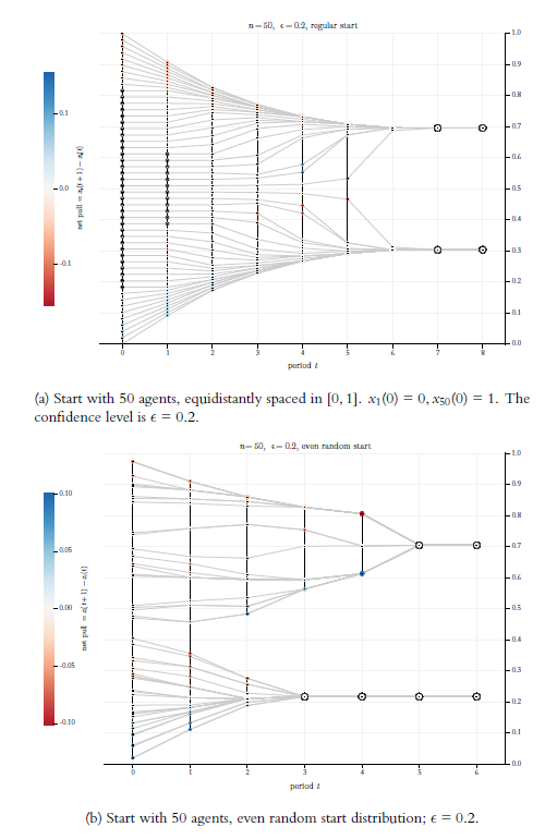
The size of the colored or grey circles indicates cluster size. A cluster is a group of agents that have the same opinion. A ‘lonely’ agent whose opinion nobody shares, is considered as a cluster of size one. Increasing circle size, means increasing cluster size.
Then there are vertical black lines. For an accurate understanding of the way they work, we introduce some terminology: A profile \(X(t)\) is an ordered profile iff
| \[ x_{1}(t) \leq x_{2}(t) \dots \leq x_{i}(t) \leq x_{i+1}(t) \dots \leq x_{n}(t)\] | \[(6)\] |
\(X(t)\) is a strictly ordered profile iff
| \[ x_{1}(t) < x_{2}(t) \dots < x_{i}(t) < x_{i+1}(t) \dots < x_{n}(t)\] | \[(7)\] |
In the following we will always start with profiles \(X(0)\) that are strictly ordered. BC-processes that start strictly ordered, always lead to ordered profiles, but these are usually no longer strictly ordered.
Now back to the black vertical lines. Suppose an ordered profile. Then the vertical lines are drawn between neighboring opinions \(x_i(t)\) and \(x_{i+1}(t)\) step by step if and only if their distance is not greater than \(\epsilon\). Thus, a vertical black line between two opinions indicates that they mutually influence each other.23
There are graphical issues: In an ordered profile, graphically, opinions that are the same, get piled up on top of each other. From the stacked opinions, we see only the top one. But we know that all the opinions below have exactly the same properties as the top one, for instance the same cluster size or the same \(\epsilon\)-insiders and outsiders. The consequence is: As long as we see an uninterrupted vertical line, there is a network in which – directly or indirectly – all agents are connected to each other. The vertical line guarantees the existence of the corresponding network paths. Thus, the visual impression is completely right—despite the fact that, technically, the vertical lines are drawn stepwise, following the indices in the ordered profile. However, there is often a problem with distinct, but very close opinions. They may be that close (and thereby mutually being among their \(\epsilon\)-insiders) that one can’t see any more the black vertical connections between them. In Figure 1a we have this problem in some densely populated, outer regions of the profiles. In this case, we have to correct the graphical impression by what we know.
The grey horizontal lines visualise trajectories and thereby take the dynamical system perspective. The black vertical lines take a network perspective: They are links between agents that mutually influence each other. Whoever is an agent on a continuous vertical black line, is a member of the same network. Both BC-processes in Figure 1 start as one network. But BC-processes are dynamical networks in which the links change over time: As the missing black line indicates, the network in Figure 1a falls apart in period \(t=6\); in Figure 1b the same happens already in \(t=2\).
To describe phenomena as the ones we see in Figure 1, let’s introduce explicitly two additional concepts that will prove useful later: An ordered profile \(X(t)\) is an \(\epsilon\)-profile (at time \(t\)) iff
| \[{} |x_{i+1}(t) - x_{i}(t)| \leq \epsilon, \text{ for } i = 1, \dots, (n-1).\] | \[(8)\] |
Without going here very much into details, one can see in the Figures 1a and 1b some typical phenomena of BC-processes: Extreme opinions are under a one-sided influence and move direction center. Therefore, the range of the profile starts to shrink. At the extremes of the shrinking (sub-)profiles, the opinions condense. Condensed regions attract opinions from less populated areas within their \(\epsilon\)-reach. In the center some opinions are pulled upwards, while others are pulled downwards. At some point \(t\), the network falls apart, the profile splits. The split sub-profiles, the two networks respectively, constitute different ‘opinion worlds’, i.e., two communities without any influence on each other. In the two split off sub-profiles opinions contract. At some point in time, in the two sub-profiles all opinions have all opinions within their confidence interval. In the next period all opinions merge into one. The consequence is stability. (Already in Hegselmann & Krause (2002) we proved that a BC-process always stabilises in finite time \(\bar t\) in the usual sense of \(X(\bar t -1)= X(\bar t)\).)
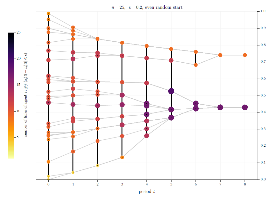
Our approach to the visualisation of BC-processes allows a two-dimensional representation of the network dynamics, whereas normally already the representation of the network for a certain time \(t\) requires two-dimensionality. As a consequence, the network dynamics itself can then only be visualised as a sequence of two-dimensional representations. Obviously, for the visualisation of BC-processes, we can manage with one dimension less. Ultimately, this is possible because all agents who have exactly the same opinion, then also have the same properties, such as their respective cluster size, links to other agents, and so on. In contrast to what is usually the case, we can therefore also stack agents that have the same opinion on top of each other without any problems: Although one then actually only sees the visualised properties of the topmost agent, one knows that all the agents below have the same properties. Figure 2 shows, how this approach can easily be used in order to visualise network (centrality) measures. As an example, Figure 2 visualises the agents’ total number of links to others.
The BC-model’s Worst Enemy: Floating-Point Arithmetic
To compute a BC-process requires to decide over and over again on sets of \(\epsilon\)-insiders and \(\epsilon\)-outsiders: Is \(|x_{i}(t) - x_{j}(t)| \leq \epsilon\), that is the decisive question. Back then in 2002 (and even quite a few years later), we considered that as a simple question, no problem for a computer. This turned out to be wrong.
Some examples of numerical disasters
Figure 3a, top illustrates a case where the computer miscalculates the set of \(\epsilon\)-insiders. For \(X(0)\) we assume what we will call a regular start profile. In such a profile \(n\) opinions are equidistantly distributed in the unit interval \([0,1]\) according
| \[{} x_{i}(0) = \frac{i-1}{n-1}, \text{ for } i = 1, \dots, n.\] | \[(9)\] |
Our example is \(n=6\) and, thus, \(X(0)= \langle 0, 0.2, 0.4, 0.6, 0.8, 1 \rangle\).24 The confidence level is \(\epsilon = 0.2\), which is exactly the distance between neighbouring opinions in \(X(0)\). As a consequence, \(X(0)\) is an \(\epsilon\)-profile as defined above, and any two neighbouring opinions are for \(t=0\) mutually members of their sets of \(\epsilon\)-insiders. The red arrow in Figure 3, top points to a segment in the profile where something went wrong: The computer miscalculates the distance between agent\(_4\) (in ascending order, the fourth agent in the start profile) and agent\(_5\), and takes the two agents that obviously are mutually \(\epsilon\)-insiders as \(\epsilon\)-outsiders. As a consequence, from \(t=1\) onwards, the whole BC-process is numerically corrupted. The correct computation is shown in Figure 3b.
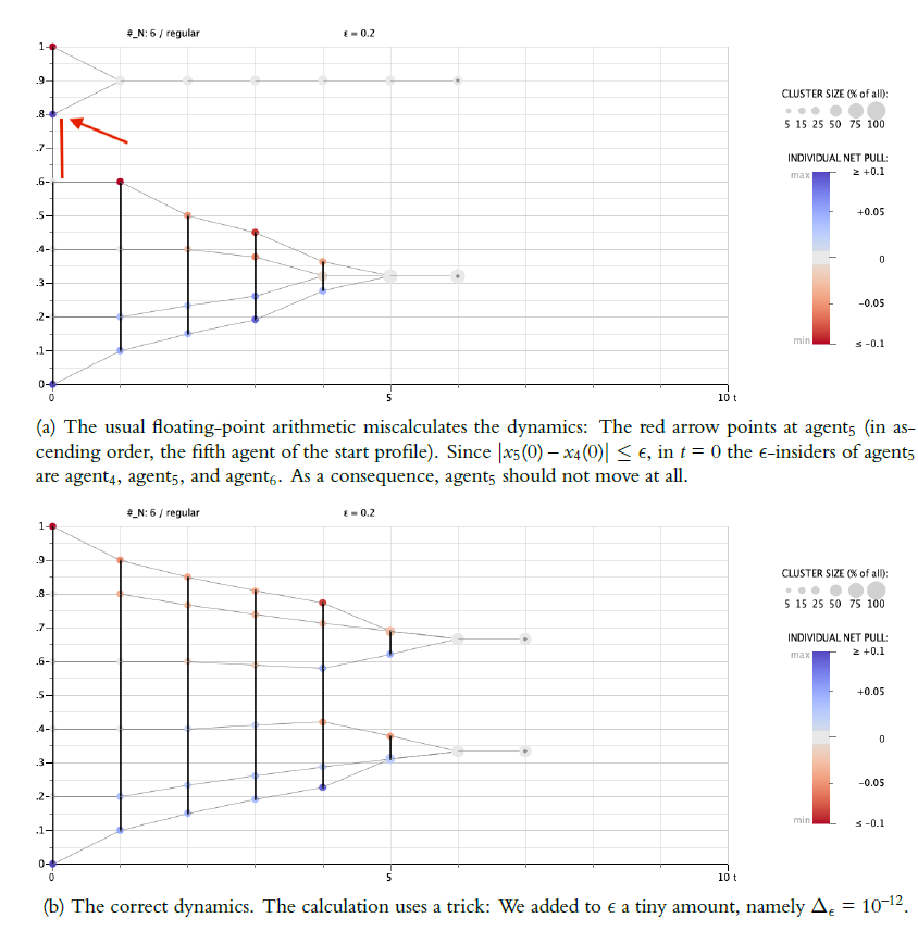
The computations that lead to the obvious mistake were done by a NETLOGO program. For the subtraction \(0.8 - 0.6\) one gets the faulty result \(0.20000000000000007\) instead of \(0.2\). The program gets it wrong by a tiny margin: \(2^{-53}\), \(10^{-17}\) respectively, that is the magnitude of the error. But that is sufficient to miss one element in two agents’ insider sets, which, then, causes follow-up errors that are 16 decimal magnitudes higher.25
What we see here, is not a problem specific to NETLOGO; it is simply an effect of the IEEE 754 standard for floating-point arithmetic, and that is the arithmetic that computers use by default.26 Floating-point arithmetic is an arithmetic with engineered numbers, often simply called floats, that approximate the uncountably infinite set of real numbers by a huge but finite set of numbers that are represented by a bit string of a predefined length, today usually 64 bits. As a consequence, almost all real numbers can’t be represented exactly, and rounding to the nearest representable number becomes ubiquitous. That, then, has consequences as we see them in Figure 3a.
One might think that the computational error in Figure 3a is a somehow artificial and rare event. Figure 4 destroys such an impression: For \(n = 51\), we set up a regular start distribution according to Equation 9. Thus, our start opinions are the decimals \(0, \ 0.02,\ 0.04,\ \dots, \ 1\). Then we compute the resulting dynamics for the decimal \(\epsilon\)-values \(0,\ 0.01,\ 0.02,\ \dots,\ 0.4\). Each process is computed until it is stabilised. Then we display the results as a diagram that we call \(\epsilon\)-diagram: Along the \(x\)-axis we have the increasing \(\epsilon\)-values, the \(y\)-axis displays for each \(\epsilon\)-value the final stable profile \(X(\bar t)\).
Given that setting, we know two things in advance: First, whatever the \(\epsilon\)-value, since the start profile is regular, there has to be a mirror symmetry along the line \(y=0.5\) in all finally stabilised profiles \(X(\bar t)\). Second, there is one agent, namely agent\(_{26}\), whose opinion should never ever change: For all \(\epsilon\)-values, and for all periods \(t=0,\ 1, \ \dots, \ \bar t\), given the symmetry of the start distribution, the opinion value of agent\(_{26}\) should always be \(0.5\)—a centrist with the centrist position (and for whom, trivially, the upward and downward pull is always balanced to zero). That is how it obviously should be. Any violation of the symmetry, any aberration of \(x_{26}(\bar t)=0.5\), is a guarantee that numerically something went wrong. (But note, and keep in mind: This kind of symmetry is only a necessary, not a sufficient condition of numerical correctness.)
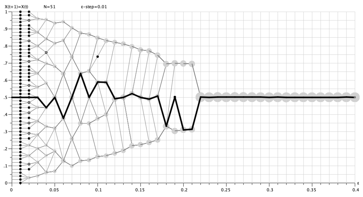
Figure 4 shows what floating-point arithmetic in our setting does—and it is a numerical catastrophy: In horizontal direction, as a kind of pseudo trajectory, light grey lines connect the final positions of the \(i\)th opinion for the stepwise increasing \(\epsilon\)-values. The thick black line is the ‘trajectory’ of the centrist agent\(_{26}\), whose opinion in numerically correct calculations will always be \(0.5\), but now—except for very small and very large \(\epsilon\)-values—almost never is. Additionally, a numerically correct computation is mirror-symmetric with regard to \(y=0.5\). But a visual inspection reveals symmetry violations all over. For \(\epsilon = 0.02\), the stabilised opinion of agent\(_{26}\) seems to be computed correctly, but other elements of \(X(\bar t)\) are not: The small filled black circle indicates a ‘cluster’ of just one agent, a black circle with a white dot inside, is a cluster of two agents. Scaled grey circles indicate cluster sizes of clusters \(\geq 3\) (for the scaling see the legend of Figure 3). For \(\epsilon = 0.02\), the cluster structure above and below agent\(_{26}\) is completely different. It is easy to extend the list of symmetry violations. In short: Figure 4 documents a major numerical disaster.27
Four computational strategies to escape numerical disaster
How to get out of the mess? There are at least four different options, three of them risky, but cheap; one of them completely safe, but costly:
- We stick to the floating-point arithmetic, but try to avoid numerical constellations that may cause numerical disasters, namely opinion values \(x_i, x_j\) with \(|x_i - x_j| = \epsilon\). We can try to avoid such constellations by an exclusive use of random start distributions: For such a distribution, the probability that there are opinion values \(x_i(0), x_j(0)\) with \(|x_i(0) - x_j(0)| = \epsilon\), equals zero. Exclusive use of random start distributions was the computational strategy in Hegselmann & Krause (2002). The approach avoids a numerical disaster in the very first updating step. However, that is no guarantee that in later periods the \(\epsilon\)-insider/outsider distinction is always correctly computed. Because of the random start, we will never see any violated asymmetries that indicate miscalculations. But indetectability does not mean non-existence. As a consequence, we get a kind of unintended and uncontrolled noise.
- We use the floating-point arithmetic even together with equidistant start distributions, but try again to avoid the critical constellations, i.e., opinions \(x_i, x_j\), such that \(|x_i- x_j| = \epsilon\). That was our computational strategy in Hegselmann & Krause (2015). There we used a very special equidistant start distribution, that we called expected value start distribution. The expected value start distribution idealises directly and ‘deterministically’ a uniform random start distribution over the range \([0,1]\): the \(i^{th}\) opinion is exactly the value, that we would get as the average of the \(i^{th}\) opinion over infinitely repeated and then ordered uniform random start distributions of \(n\) opinions. An expected value distribution of \(n\) opinions starts with
Working with an expected value start distribution instead of repeated randomly started runs, is sometimes a fruitful methodological approach: It minimises the danger to blurr interesting effects by averaging. Additionally, if there is an effect that needs explanation, one can directly study the unique single runs that produced the effect. In Hegselmann & Krause (2015) we applied that approach (as we think successfully) and used a start distribution according to Equation 10 with \(n=50\). As a consequence, the distance between neighbouring opinions is always \(1/51 = 0.\overline{0196078431372549}\). Given that distance, none of the 50 opinions in \(X(0)\) is for any \(\epsilon = 0.01,0.02,...,0.4\) at the bounds of confidence of any other opinion. As to the very first updating step, we are therefore computing on safe ground. And as to the later periods, there is some evidence for justified hope: If we calculate an \(\epsilon\)-diagram as the one in Figure 4, but now for an expected value start distribution with \(n = 50\), then we get a diagram that is completely mirror symmetric (cf. 2015 p. 487). As said, however, symmetry is only a necessary, not a sufficient condition for numerical correctness. Additionally, the symmetry check is a check by visual inspection only, and there may be asymmetries that are too small to catch the eye.28\[ x_{i}(0) = \frac{i}{n+1}, \text{ for } i = 1, \dots, n.\] \[(10)\] - The problem in the dynamics in Figure 3 is that an \(\epsilon\)-insider is mistaken as an outsider; the problem is not that an \(\epsilon\)-outsider is mistaken as an insider. This asymmetry is typical and suggests a numerical trick: We stick to floating-point arithmetic, but as a precaution we always add a tiny amount \(\Delta_\epsilon\) to \(\epsilon\)—sufficiently much to get the set of \(\epsilon\)-insiders right. The precaution works astonishingly well. In the last years, in many contexts and almost routinely, we used a \(\Delta_\epsilon = 10^{-12}\). The (correct) process in Figure 3, bottom is calculated by a NETLOGO program that uses the trick.29 That the trick works, can be checked by a safe method that does not use the trick. The method will be described below. But here and in general we would like to know (and often have to know) why, when and for which \(\Delta_\epsilon\)-values the trick works without producing the complimentary mistake: taking an \(\epsilon\)-outsider for an insider. It is a trivial task, to calculate for a process \(\langle X(0),\epsilon \rangle\) a value for \(\Delta_\epsilon\) that would numerically corrupt the process right from the start. If \(X(0)\) is an equidistant start distribution, it might even happen that the numerical corruption that is caused by a too large \(\Delta_\epsilon\), works symmetrically and, therefore, is practically undetectable.
- We abandon floating-point arithmetic altogether, and resort to an exact alternative: fractional arithmetic that restricts itself to the exclusive use of rational numbers as fractions of integers. Such numbers can always be exactly represented. All computations are then done as fractional operations. In the computation of a BC-process that easily leads to numerators and denominators in the hundreds of millions—an expression swell (a well known general problem of the exact fractional approach) that requires a permanent and complicated search for expression simplifications. To avoid necessities for rounding since otherwise numerators and denominators become too big to be representable by a bit string of predefined length (for instance the usual 64 bits format), we need to be able to use integers of arbitrary length.
Such a fractional approach with integers of arbitrary length is technically possible. With fractional arithmetic, we operate numerically on completely safe ground. But the solution comes at a cost in terms of computation speed: Fractional arithmetic is comparatively slow and takes much more time than floating-point arithmetic. For tasks that can reasonably be done by both methods, the safe fractional method may easily need one or two orders of magnitudes more time. MATHEMATICA and JULIA allow computations in fractional arithmetic. NETLOGO does not.
In the next section we will turn to the non-monotonicities that we overlooked in Hegselmann & Krause (2002). Soon it will become clear, that analysis and understanding of the non-monotonicities requires computationally a fractional approach.
A New Key Concept: \(\epsilon\)-Switches
The best way to understand the wild behavior of BC-processes \(\langle X(0),\epsilon \rangle\) in detail, is to start with very simple (and seemingly unrelated) questions: Given a certain start distribution \(X(0)\), how many different processes \(\langle X(0),\epsilon \rangle\) exist? How many values of \(\epsilon\) are there that make a difference? Is it a finite number, an infinite number? And how can we find them all, or at least some of them?
The example \(X(0) = \langle 0, 0.18, 0.36, 0.68, 1.0 \rangle\)
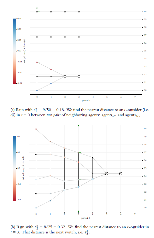
As an example, let us take the start distribution \(X(0) = \langle 0, 0.18, 0.36, 0.68, 1.0 \rangle\).30 For \(\epsilon = 0\), simply nothing will happen. Since \(X(0)=X(1)\), the dynamics is stable in \(t=1\). Now we start to increase the value of \(\epsilon\). What is the smallest value of \(\epsilon\) that makes a difference? An \(\epsilon = 0.1\) would not make any difference—-still, nothing would happen, the same sets of \(\epsilon\)-insiders, the same trajectories as for \(\epsilon = 0\). Obviously, the very first strictly positive \(\epsilon\)-value that really makes a difference, is an \(\epsilon\)-value that equals the distance to a nearest \(\epsilon\)-outsider in the profile \(X(0)\). In our example that is the distance \(0.18\). We find this distance between two pairs, namely for \(|x_2(0) - x_1(0)|\) and \(|x_3(0) - x_2(0)|\). Figure 5a shows the dynamics for \(\epsilon = 0.18\). Compared to the situation for \(\epsilon = 0\), the value \(\epsilon^*= 0.18\) is a kind of switch for the given start distribution: Once \(\epsilon\) reaches that value, the insider/outsider composition and thereby the network structure changes. At least one new link between two agents is established that was not there before. As a consequence, we get, compared to the process \(\langle X(0),\epsilon=0 \rangle\), a different BC-process, namely the one in Figure 5a.
By inspection of Figure 5a it is clear, that a further increase of \(\epsilon\) to \(\epsilon = 0.2\), would not make any difference—we would get exactly the same process that we see already in Figure 5a, the process that is generated by the first switch. The next and nearest larger \(\epsilon\) that again changes the process, is the one that is equal to the distance to the nearest \(\epsilon\)-outsider that we can find in the entire process \(\langle X(0),\epsilon = 0.18 \rangle\) of Figure 5a. Such an \(\epsilon\) is a second switch, that again establishes a new link that did not exist before. By inspection of Figure 5a, it is clear which \(\epsilon\)-value that is: It is an \(\epsilon\) that equals the distance between agent\(_3\) and agent\(_4\) and the distance between the agent\(_4\) and agent\(_5\) right at the start, namely \(|x_5(0) - x_4(0)| = |x_5(0) - x_4(0)| = 0.32\). The green vertical lines in Figure 5a show the two distances to nearest \(\epsilon\)-outsiders. We make this value our new starting point for finding the nearest larger \(\epsilon\)-value that makes a difference, and so forth.
More precisely, the next and nearest \(\epsilon\)-outsider we are looking for, is the minimum element in the set of all distances to \(\epsilon\)-outsiders of all agents over all periods \(t\) for the BC-process \(\langle X(0), \epsilon \rangle\). To that minimum element we will refer as \(\delta_{min}^{out} \bigl(X(0), \epsilon \bigr)\). In formal terms:
| \[ \delta_{min}^{out} \bigl(X(0), \epsilon \bigr) = min \Big\{|x_{i}(t) - x_{j}(t)| \Big \vert \, t = 0, 1, \dots, \bar t \,; \, i = 1,\dots, n; \, j \in O\bigl(i,X(t), \epsilon \bigr) \Big\}\] | \[(11)\] |
Search for \(\epsilon\)-switches: The algorithm that finds them all
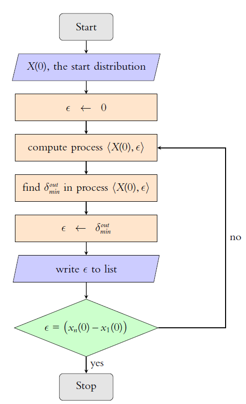
At this point, probably inevitably, one gets the idea of an algorithmic search for minimal distances to \(\epsilon\) outsiders. For a given start distribution \(X(0)\) we start with \(\epsilon = 0\), and then search for \(\delta_{min}^{out}\), the distance to a nearest \(\epsilon\)-outsider. Doing that, we find \(\epsilon_1^*\), the first switch that, compared to the process \(\langle X(0), \epsilon = 0 \rangle\), makes a difference. For our start distribution we find \(\epsilon^*_1 = 0.18\). That is the start of a loop. Now we search \(\delta_{min}^{out}\) in \(\langle X(0), \epsilon_1^* \rangle\) and thereby find the second switch \(\epsilon_2^* = 0.32\). This second switch generates the BC-process \(\langle X(0),\epsilon^*_2 \rangle\) shown in Figure 5b. If we go, period by period, through all the distances to \(\epsilon\)-outsiders, we will find (marked by the green vertical line) the distance to the nearest \(\epsilon\)-outsider in \(t=3\), namely the distance between \(x_5(3)\) and \(x_3(3)\). That distance is the third switch \(\epsilon_3^*\). We use that switch to compute the process \(\langle X(0),\epsilon^*_3 \rangle\), in which, then, we search for \(\delta_{min}^{out}= \epsilon^*_4\), and so the loop goes on.
As we know directly from \(X(0)\) the first switch, so we know directly from \(X(0)\) the largest switch, namely the distance \(x_n(0)- x_1(0)\), the width of the start profile. For \(\epsilon^* = \big(x_n(0)- x_1(0)\big)\), all agents are linked to all agents already in \(t=0\). In \(t=1\) they have all the same opinion, and the process is stable in \(t=2\). All \(\epsilon > \epsilon^*\) have the same effect, and can’t make any further difference. Therefore, the search algorithm can stop once \(\epsilon^* = \big(x_n(0)- x_1(0)\big)\) is reached. The flowchart in Figure 6 visualises the algorithm.
Here we should stop immediately because of flashing red lights: In Section 3.1 we saw, that the most numerically dangerous situation is a constellation in which opinions lie exactly on the bounds of confidence of other opinions. But obviously our search algorithm creates exactly this type of situation over and over again: Each switch generates a BC-process in which at least two agents have opinions that are exactly and mutually at the upper or lower bounds of their confidence interval. In other words: Without precautions, our algorithm is a recipe for a numerical disaster.
What to do? Of the four options we discussed as possible solutions in Section 3.2, the first two are not applicable: By design and for good reason, our algorithm creates the constellation that the two options try to avoid. The third option adds a tiny amount \(\Delta_\epsilon\) to \(\epsilon\) to avoid the error of missing an \(\epsilon\)-insider. But this can lead to a complementary problem, namely mistaking an \(\epsilon\)-outsider for an \(\epsilon\)-insider—and we simply do not know what \(\Delta_\epsilon\) would be too much. Consequently, there is no other option than the costly solution of option four: All computations of our algorithm have to be done as fractional arithmetic, and it has to be done with integers of arbitrary length. This is exactly what we are going to do. And it is also what we have already done without mentioning it in the calculation of the processes in Figure 5above. Otherwise we would be heading for numerical disaster with the second switch: Looking at 5a, we see that the second switch equals \(0.32\). But when using floating-point arithmetic, the computer get’s it wrong. For \(|1.0 - 0.68|\), i.e., the distance between agent\(_5\) and agent\(_4\) in \(t=0\), we get \(0.31999999999999995\); for \(|0.68 - 0.36|\), i.e., the distance between agent\(_4\) and agent\(_3\), we get \(0.32000000000000006\). Both results are obviously wrong. Since the first distance is smaller than the second, the algorithm would return \(\epsilon_2^* = 0.31999999999999995\). In the next step we would get \(\epsilon_3^* = 0.32000000000000006\)—and we have a completely corrupted list of switches right from the start.
Therefore, from now on, we will compute consistently on numerically safe ground: fractional arithmetic, and nothing else. Table 1 gives an example. It shows all exact fractional results for the BC-process that starts with our example start distribution and an \(\epsilon\)-value that equals \(0.32\), in fractional terms \(8/25\), a value that we already identified as \(\epsilon_2^*\), the second switch for the given start distribution.
| agent | \(t=0\) | \(t=1\) | \(t=2\) | \(t=3\) | \(t=4\) | \(t=5\) | \(t=6\) |
|---|---|---|---|---|---|---|---|
| 1 | 0/1 | 9/100 | 203/900 | 569/2160 | 63307/172800 | 1669/3840 | 1669/3840 |
| 2 | 9/50 | 9/50 | 203/900 | 569/2160 | 63307/172800 | 1669/3840 | 1669/3840 |
| 3 | 9/25 | 61/150 | 407/1200 | 573/1600 | 63307/172800 | 1669/3840 | 1669/3840 |
| 4 | 17/25 | 17/25 | 289/450 | 6269/10800 | 18719/43200 | 1669/3840 | 1669/3840 |
| 5 | 1/1 | 21/25 | 19/25 | 631/900 | 13841/21600 | 1669/3840 | 1669/3840 |
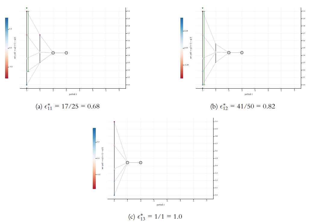
When we run the algorithmic search for the \(\epsilon\)-switches of our example start distribution \(X(0)\), we get a total of 13 switches. They are listed in Table 2. The table displays the exact rational values and their decimal representation as floating-point numbers (64 bits). The 13 switches allow to initialise 13 different BC-processes. The first two are shown in Figure 5. Figures 7 and 8 show the remaining 11 possible BC-processes. The 13 processes exhaust all possibilities for BC-processes that start with \(X(0) = \langle 0, 0.18, 0.36, 0.68, 1.0 \rangle\)—-nothing else is possible.
| switch | exact | float64 |
|---|---|---|
| \(\epsilon_1^*\) | 9/50 | \(0.18\) |
| \(\epsilon_2^*\) | 8/25 | \(0.32\) |
| \(\epsilon_3^*\) | 4939/14400 | \(0,342986111111111\) |
| \(\epsilon_4^*\) | 9/25 | \(0.36\) |
| \(\epsilon_5^*\) | 3/8 | \(0.375\) |
| \(\epsilon_6^*\) | 29/75 | \(0.386666666666667\) |
| \(\epsilon_7^*\) | 339/800 | \(0.42375\) |
| \(\epsilon_8^*\) | 1/2 | \(0.5\) |
| \(\epsilon_9^*\) | 107/200 | \(0.535\) |
| \(\epsilon_{10}^*\) | 16/25 | \(0.64\) |
| \(\epsilon_{11}^*\) | 17/25 | \(0.68\) |
| \(\epsilon_{12}^*\) | 41/50 | \(0.82\) |
| \(\epsilon_{13}^*\) | 1/1 | \(1.0\) |
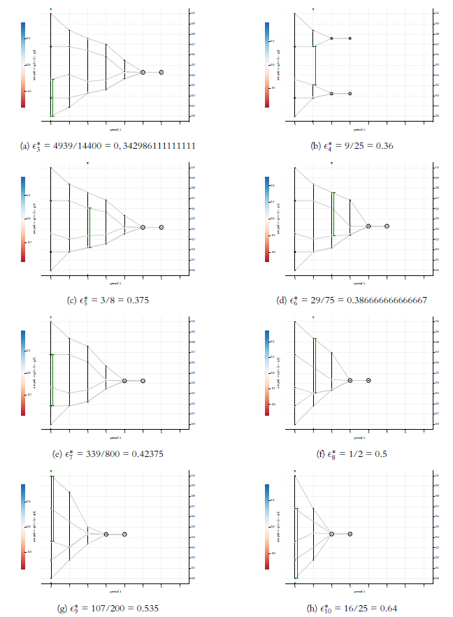
Comparing the 13 possible processes, the probably most surprising phenomenon regards the switches \(\epsilon_3^*\), \(\epsilon_4^*\), and \(\epsilon_5^*\) (cf. Figures 7a, 7b, and 7c): For \(\epsilon_3^*\) the process reaches a consensus. But for the larger \(\epsilon_4^*\) the consensus is breaking up—a clear cut case of a counter intuitive non-monotonicity. For the next switch \(\epsilon_5^*\) we get consensus again. Though in a less spectacular way, all 13 switches make a difference for the trajectories of the BC-processes that they generate. Going through the 13 runs in Figures 5, 7, and 8, we see a huge variety of differences:
- The number of final clusters may decrease (\(\epsilon_1^* \rightarrow \epsilon_2^*\), \(\epsilon_4^* \rightarrow \epsilon_5^*\)) or increase (\(\epsilon_3^* \rightarrow \epsilon_4^*\)).
- The width of the final cluster structure, i.e., \(x_n(\bar t)-x_1(\bar t)\), may decrease (\(\epsilon_1^* \rightarrow \epsilon_2^*\), \(\epsilon_4^* \rightarrow \epsilon_5^*\)) or increase (\(\epsilon_3^* \rightarrow \epsilon_4^*\)).
- The exact position of a consensus in \([0,1]\) may change (for instance \(\epsilon_5^* \rightarrow \epsilon_6^*\), \(\epsilon_{11}^* \rightarrow \epsilon_{12}^*\)).
- For some \(t < \bar t\), the width of \(X(t)\), i.e., \(x_n(t)-x_1(t)\), may decrease (for instance \(\epsilon_2^* \rightarrow \epsilon_3^*\) for \(t=4\)) or increase (for instance \(\epsilon_3^* \rightarrow \epsilon_4^*\) for \(t=3\)).
- A profile \(X(t)\) that was an \(\epsilon\)-profile beforehand, may get an \(\epsilon\)-split (for instance \(\epsilon_3^* \rightarrow \epsilon_4^*\) for \(t=1\)); a profile that had an \(\epsilon\)-split, may become an \(\epsilon\)-profile (for instance \(\epsilon_4^* \rightarrow \epsilon_5^*\) for \(t=1\)).
- The time to stabilisation may decrease (\(\epsilon_3^* \rightarrow \epsilon_4^*\), \(\epsilon_5^* \rightarrow \epsilon_6^*\), \(\epsilon_7^* \rightarrow \epsilon_8^*\), \(\epsilon_9^* \rightarrow \epsilon_{10}^*\), \(\epsilon_{12}^* \rightarrow \epsilon_{13}^*\)) or increase (\(\epsilon_1^* \rightarrow \epsilon_2^*\), \(\epsilon_4^* \rightarrow \epsilon_5^*\)).
The observed differences in the trajectories are not mutually exclusive, and probably there are more differences than the ones that I listed.
Beyond the example: General observations and conjectures on \(\epsilon\)-switches
The algorithm that finds the \(\epsilon\)-values that make a difference in our example start distribution can be applied to any start distribution. I have applied it to countless start distributions—random, regular, expected value, lots and lots of start distributions I had found interesting for some reason. Result: the algorithm always listed finitely many increasingly large switches, and then stopped. As analytical reflections already showed for the example in Section 4.1, the first switch equals the smallest distance between neighbouring opinions in the (strictly ordered) start profile. The last switch found and at the same time the largest switch equals the width \(x_n(0)-x_1(0)\) of the start profile. The fact that the algorithm stops, and thereby leads to a finite list of switches, is not self-evident (at least not for me): perhaps there could be an infinite number of switches between a smallest and a largest switch. However, in none of my computational experiments was this the case. But I have no proof that the number of switches is always finite.
The finite list of strictly increasing \(\epsilon\)-switches that the algorithm finds, leads to a complete segmentation of \([0,1]\) by the following sequence of intervals (right-open except for the last one):
| \[ \langle \ [0,\epsilon_1^*)\ , \ [\epsilon_1^*,\epsilon_2^*)\ ,\ \dots, \ [\epsilon_{s-1}^*,\epsilon_s^*) \ , \ [\epsilon_s^*,1] \ \rangle \ \text{with} \ 0 < \epsilon_1^* < \epsilon_2^*,\ \dots,\ \epsilon_s^* \leq 1.\] | \[(12)\] |
The list of \(\epsilon\)-switches yields a gapless sequence of segments \([\epsilon_k^*, \epsilon_{k+1}^*)\). In what follows, we will often speak of predecessor or successor switches. That then refers to the switch \(\epsilon_{k-1}^*\) or \(\epsilon_{k+1}^*\) that in the ordered list of switches precedes or succeeds \(\epsilon_k^*\).
For any given start distribution, all \(\epsilon\)-values from the same segment lead to exactly the same BC-process; processes with \(\epsilon\)-values from different segments, on the other hand, are never the same. Overall, for any given start distribution, it is possible to get a complete overview of which BC-processes are possible at all. We can, switch by switch, go through all possible processes and look for properties that interest us:
- Is a consensus being destroyed again?
- Is the number of final clusters increasing again?
- Is the final profile width increasing again?
- How long does it take to stabilise?
- Which switch produces the first consensus that is not destroyed by any subsequent switch?
- In which period was the next switch found?
The answers to all these questions can be generalised in a precise sense: Assuming that the \(k^{th}\) switch \(\epsilon_k^*\) of a start distribution \(X(0)= x_1(0), \dots , x_i(0), \dots, x_{n}(0)\) destroys a consensus, then this is also true for the \(k^{th}\) \(\epsilon\)-switch of a start distribution \(X^\diamond (0)\), which we get from \(X(0)\) by a transformation of the form
| \[ x_i^\diamond(0) = \alpha \cdot x_i(0) + \beta, \text{ with } \alpha > 0 \text{ and } \alpha, \beta \in \mathbf{R}\] | \[(13)\] |
In our example above in Section 4.1, only once a consensus is destroyed by the next larger switch. There are much wilder BC-processes: For the same start distribution, it may happen several times that a consensus is destroyed again by a successor switch. There are several ways to demonstrate that, for instance by the analysis of a major set of random start distributions. Here in this article I will use another strategy: We will look at all regular start distributions for \(n=2, \dots, 50\). Throughout the text, a regular start profile with \(n\) agents will be occasionally referred to as \(X_{r,n}(0)\). In a first step, Figure 9 shows their respective number of \(\epsilon\)-switches. The \(x\)-axis shows the \(n\)-values, the \(y\)-axis the number of \(\epsilon\)-switches that our algorithm finds for a regular start distribution with the respective \(n\). As shown and motivated in Appendix B, Universal characteristics of equidistant start distributions, the number of switches is universal: Whatever the specific equidistance \(c\), whatever the range of the profile, any equidistant start profile with \(n\) agents has the same number of switches. And even more: For all equidistant start distributions with a given \(n\), the properties of the \(k^{th}\) of the \(s\) switches are always the same.31 Thus for example, what we see in Figure 9 also holds for an expected value start distribution as it would for a start distribution with an equidistance of \(c=1\), thereby leaving the unit interval as our opinion space.32
In Figure 9 the blue graph connects the numbers of \(\epsilon\)-switches for consecutive even numbers of \(n\); the red graph does that for odd numbers. The grey graph connects directly the \(y\)-values for consecutive values of \(n\). For \(n=49\) the algorithm finds \(624\) switches, for \(n=50\) there are \(607\).
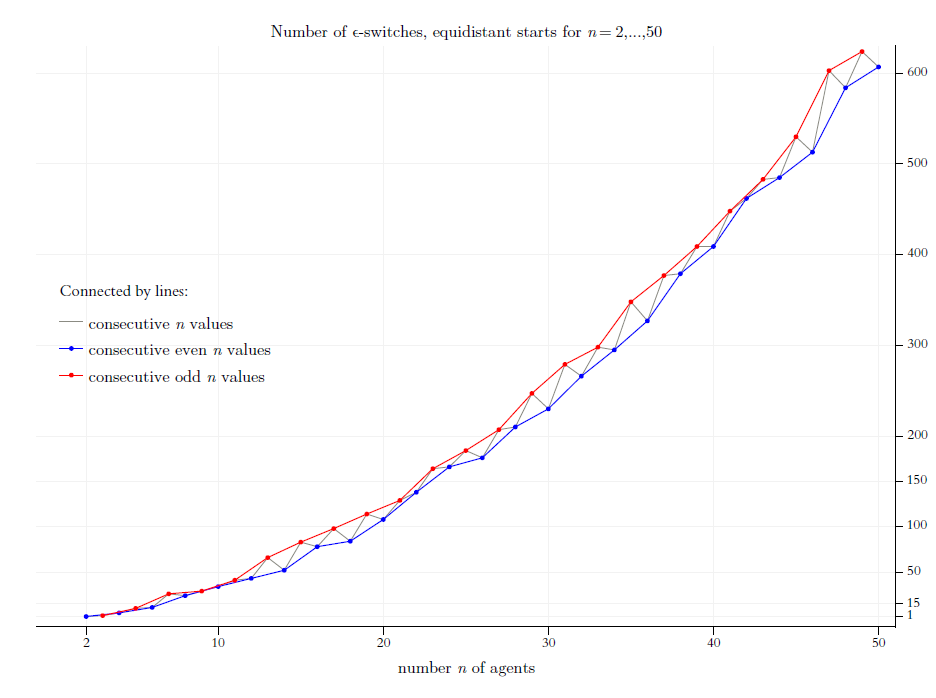
By inspection of Figure 9 we see: For increasing even values of \(n\), and as well – but separately – for increasing odd values of \(n\), the number of switches increases monotonically. And in both cases the increase is more than linear.
In Figure 10, we start focusing on the ‘wild’ behavior of BC-processes: We look for switches that break up a consensus and turn the consensus into strict polarisation (i.e., a final stable cluster structure with exactly two clusters). Figure 10 shows how many such switches there are. As in Figure 9, the \(x\)-axis shows the increasing values \(n=2, \dots, 50\) of the regular start distributions that the algorithm searches for such switches. The \(y\)-axis shows the results. Again, via the colors blue and red, we distinguish even and odd values of \(n\). If you look at Figure 10, two things immediately jump to the eye: For even values of \(n\) there are quite a lot of destroyed consents; for odd values there is none. As to the even \(n\)-values, for \(n=40\) and \(n=46\) it is six times each that a consecutive switch leads to polarisation while the predecessor switches generated consensus. And, by extrapolation, it looks as if (though stepwise) for increasing (even) values of \(n\) there are higher numbers of such cases.
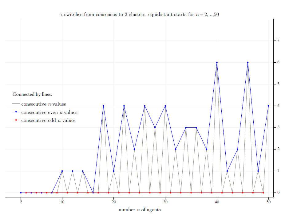
Why are there no such cases for odd values of \(n\)? The explanation is closely related to our earlier discussion of symmetrical start profiles (cf. Section 3.1): If we start with a regular profile, and \(n\) being an odd value, then there is always a centrist agent exactly in the middle of the opinion profile (possibly as a member of a centrist cluster \(>1\)). Whatever the confidence level \(\epsilon\), the centrist agent will always stay in the center. As a consequence, a constellation with an empty center, as required for a strict polarisation, is not possible.
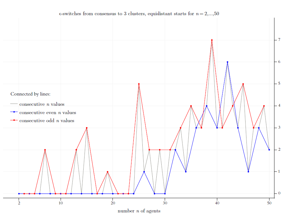
Figure 11 focuses on a second, somehow even more dramatic type of destroyed consent: The consecutive switch generates three final clusters. Now the odd values of \(n\) seem to be much better in producing such a structure. For even \(n\)-values \(<26\) it never occurs that after a consent the next switch generates a final structure of three clusters. However, for \(n=42\) it happens six times. Based upon our perfect and complete knowledge of all switches, we can also look for switches that turn a consent into a final cluster structure with more than three clusters. (But so far I never found such a case in any regular start distribution.)
The Figures 9 to 11 show for regular start profiles \((n=2,3, \dots, 50)\) the number of their \(\epsilon\)-switches and how many of them destroy consents. But the figures do not give any information about the exact positions of the switches in the interval \([0,1]\). Figure 12 shows by a new type of diagram all sorts of non-monotonicities together with the positions of the switches that are generating them. On the \(x\)-axis of Figure 12 we have the complete range of possible \(\epsilon^*\)-values, i.e., \([0,1]\). The \(y\)-axis shows the increasing values of the number \(n\) of agents in a regular start profile \(X_{n,r}(0)\). Thus, each switch is a certain point \(\langle x,y \rangle\) in the coordinate system thus given.
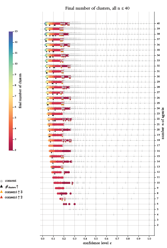
At this point, we place a colored circle that indicates by its color the specific feature that we want to visualise with the diagram, namely the final number of clusters. As the \(y\)-axis represents the \(n\) values, all the switches of a start distribution for a given \(n\) are lined up horizontally. The colormap together with legends (both to the left) give the information how to read the specific diagram. A bit above the often overlapping, horizontally lined up circles, there are very small black dots. The dots indicate the exact position of the switch directly below. Due to the minimal size of the black dots, they overlap much less (if at all) than the colored circles. As a consequence, we get a sense for the different densities with which the switches are distributed in the interval \([0,1]\).
In Figures 9 to 11 we looked at regular start profiles with \(n=2,3, \dots, 50\); in Figure 12 we reduce the range to \(n=2,3, \dots, 40\). The reason is better visibility and readability of details. (Admittedly, even after the range reduction the graphics is a bit packed.)
Already a cursory glance at Figure 12 shows that the positional structure of the switches clearly has a pattern. For each \(n\), the very first switch has an \(x\)-axis position at \(\epsilon^*_1 = 1/(n+1)\), i.e., the characteristic equidistance of the regular start distribution with \(n\) agents (cf. Equations 9 and 23). That equidistance is, obviously, at the same time the minimum distance to an \(\epsilon\)-outsider in all processes \(\langle X(0), \epsilon=0 \rangle\). As a consequence, for increasing values of \(n\), the first switch gets smaller and smaller, moves left direction \(0\), and, thereby, produces a convex-shaped curve with regard to the positions of the very first switches. As well trivial is the position of the largest switch: from our analytical reflections above we know that the largest switch of a regular start distribution is always \(1\). What stands out most clearly, is a certain positional pattern in between the first and the last switch: At the beginning the positions of the switches look chaotically distributed. But, as we get farther right, the positional distribution becomes completely regular. At least for \(n \geq 10\), a first type of positional regularity starts for switches greater \(\approx 0.4\): There the distance between consecutive switches becomes equidistant, and the size of the equidistance seems to depend upon \(n\), namely decreasing with \(n\). A second type of regularity then starts a bit farther right, namely for switches greater than \(0.5\): Consecutive switches are positioned equidistantly, but with (about?)the size of the equidistance that we see to the left of \(0.5\). Again, the size of the equidistance seems to decrease with \(n\). And finally, whatever the value of \(n\), \(\epsilon = 0.5\), i.e., the middle of the range of opinions for a regular start profiles, is always a switch. In terms of their density, the switches are very much concentrated in the initial range of possible values between \(1/(n+1)\) and \(\approx 0.35\). At the same time, in that region their positional distribution does not seem to follow any type of a regular pattern.
Figure 12 focuses on the final number of clusters that the switches generate. That number is indicated by a color according to the colormap to the left. Consents, i.e., the cases of just one final cluster, get a special treatment: They are indicated by grey circles that are also a little bit smaller than the other colored circles. And the grey circles are drawn last, after all other circles are already drawn. That makes consents more easily visible. Then there are upwards directed triangles in Figure 12. They mark switches that produce specific non-monotonicities: Black triangles hint to switches that lead to final cluster structures with more clusters than the predecessor switch did. An orange triangle marks the switches that, after a consent under the predecessor switch, lead to three clusters. A red triangle hints to a switch that, after a consensus, leads to strict polarisation, i.e., two clusters. The black triangles are always drawn first. As a consequence (and on purpose), they are overdrawn by orange or red triangles in cases of destroyed consents. Thus, the markers of these cases are always visible.
A careful inspection of Figure 12 makes it very clear: For all \(n\), there is always a switch that leads to a consensus that is final in the sense: No successor switch destroys the consent.33 However, the transition from a final plurality (i.e., a major number) of clusters to a final consensus (just one cluster) is wild, chaotic, and non-monotonic. Only for a few values of \(n\), the first consensus switch is also the final one. Normally, from switch to switch, many times the number of final clusters decreases and increases again. The most dramatic cases of this type are the many cases of a back-and-forth of consensus and dissent (the latter in the sense of polarisation or a final structure with three clusters). And there is a difference between even and odd values of \(n\): For odd values the final consensus switch comes for significantly smaller \(\epsilon\)-values.
Separate from the main text, Appendix B summarises, in a more formal and technical language, analytical notes and observations on universal characteristics of equidistant start distributions. The appendix also contains additional figures. In the style of Figures 9 to 11: (a) the number of switches that lead to more final clusters than under the respective predecessor switch; (b) the number of switches that lead to final profile widths that are greater than under the predecessor switch. Three further figures, similar in style and structure to Figure 12, show for all switches (a) the final profile widths, (b) the times to stabilisation, and (c) the period in which the switch was found. (Again, what follows in the main text will be understandable without a reading of the appendix.)
A new BC-research tool: \(\epsilon\)-Switch diagrams
Figure 12 gives a general overview: We see the positions of switches and get to know especially the ones that are responsible for certain non-monotonicity effects. But we do not see in detail where exactly the final clusters are located or what the width of a final profile is. For that we need another type of diagram.
From \(\epsilon\)-diagrams to \(\epsilon\)-switch-diagrams
Above, in Figure 4 we used a so called \(\epsilon\)-diagram: For stepwise increasing \(\epsilon\)-values (\(x\)-axis, step size is \(0.1\)) it shows the final cluster structure (\(y\)-axis). Given what we know now, an improved version of this diagram could show the details much more to the point (even in a very literal sense): By our search algorithm we get perfect knowledge of all \(\epsilon\)-switches, and we can compute such a list for any profile \(X(0)\). But then we should also show the final cluster structure solely and exclusively for the \(\epsilon\)-switches, i.e., the \(\epsilon\)-values that make a difference. We will call the improved diagram an \(\epsilon\)-switch diagram (for short switch diagram). Figure 13 is an example.
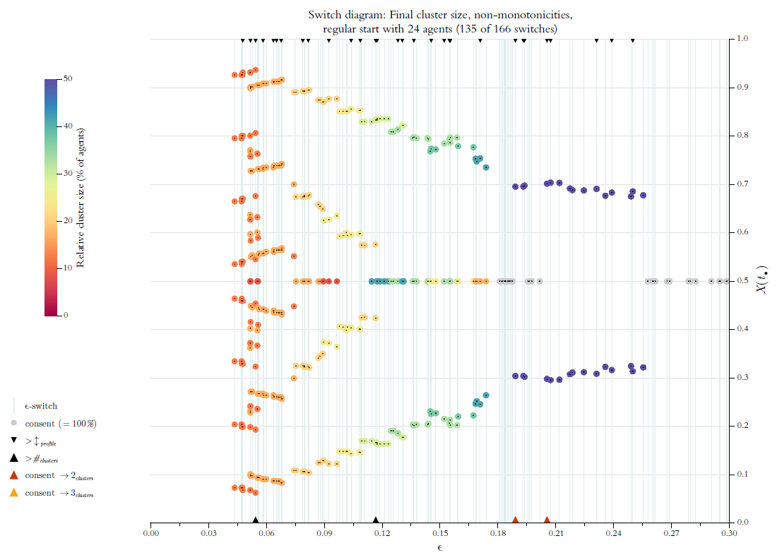
The thin vertical lines indicate the positions of switches. Colored circles show the position and the relative size of the final clusters. A consensus cluster is colored grey and drawn last. Tiny black dots in the centre of the circles mark the exact position of the respective cluster. At the same time the dots help to distinguish and separate clusters even if their circles overlap. The dots are drawn last. The diagram only shows the switches \(\leq 0.3\). Here that regards \(135\) of a total of \(166\) switches. From Figure 12 we know that with \(\epsilon^* \leq 0.3\) we are already behind the final consensus switch.
In Figure 13, upward and downward triangles support the visual detection of non-monotonicities. The upward directed triangles are used in the same way as in Figure 12: Black triangles mark switches that generate structures with more final clusters than the predecessor does. An orange triangle marks switches that, after a consent, lead to three clusters. A red triangle hints to a switch that turns consent into strict polarisation. Again, the black triangles are drawn first. The smaller, downward directed triangles along the upper end of the coordinate system mark switches that, compared to their predecessors, generate an increasing width of the final profile. All in all, \(\epsilon\)-switch diagrams are the more accurate successors of the 3-dimensional frequency distribution that we used in (Hegselmann & Krause 2002) (Figure 3, page 11).34
It is a direct consequence of the definition of an \(\epsilon\)-switch that on the \(x\)-axis to the right of \(\epsilon = 0\) there is an empty region without any switch: By definition, there is no switch smaller than the equidistance of \(X_{24,r}(0)\), and that is \(1/(n+1)=1/25=\epsilon_1^*\). For an expected value start distribution with \(24\) agents we would get the same diagram, except for a left shift of all switches by the factor \(23/25\).35
Figure 13 is a switch diagram for a regular \(X(0)\) with \(24\) agents. Figure 14 is the same type of diagram, but now for \(25\) agents. By a comparison of the two figures, we see now more in detail the typical difference between even and odd values of \(n\): In the even case, the final consensus switch comes much later than in the odd case. And, second, the phase in which there normally are two big outer clusters, is much longer in the even case. We postpone an answer to the questions: How comes?
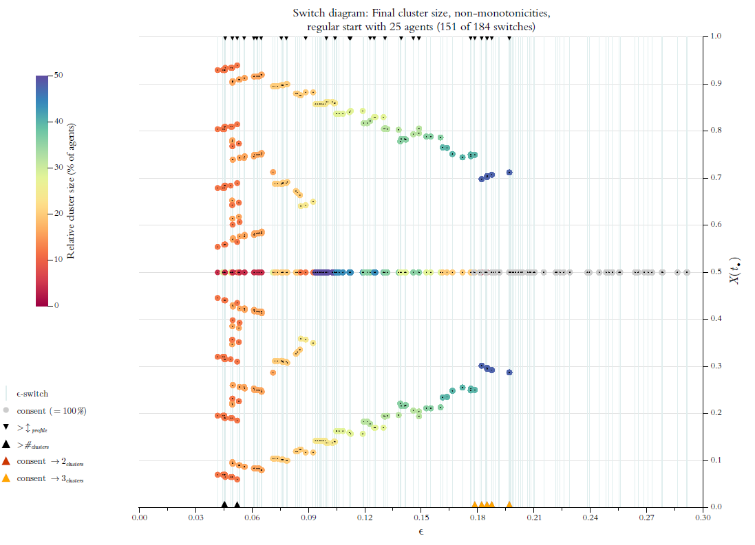
From \(\epsilon\)-switch-diagrams to \(\epsilon\)-switch-movies
Switch diagrams are an extremely helpful tool to better understand BC-processes. An important next step is to produce for \(n=2,3, \dots\) a sequence of switch diagrams. By a careful inspection of such a sequence, we can directly see the effects of an increasing number of agents. Already the global overview in Figure 12, and, as well, the switch diagrams of Figures 13 and 14 suggest to distinguish between even and odd values of \(n\). Therefore we computed two sequences, the ‘even’ switch diagram sequence for \(n=2, 4, \dots, 80\); and the ‘odd’ sequence for \(n=3, 5, \dots, 79\).
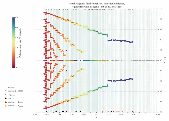
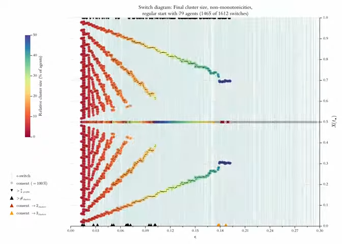
Going slowly through the consecutive switch diagrams (\(n\)-value by \(n\)-value, doing it back and forth), the most prominent phenomena seem to be:
- Overall, by and large, for all \(n\) (even or odd) there is a non-monotonic tendency to a decreasing number of final stable clusters, a decreasing profile width, a non-monotonic transition from plurality (or fragmentation) to polarisation, and finally consensus. But this overall tendency is really ‘wild’: It is, with few exceptions, completely normal, that subsequent switches lead again to increasing profile widths, increasing numbers of clusters, destroy a consensus, thereby producing a strict polarisation with an empty centre (for even values of \(n\)), or, less strict, a constellation with two big outer clusters and a small centre cluster (for odd \(n\)-values).
- As to polarisation, there is another difference between strict polarisation in the even case, and the less strict polarisation in the case of odd \(n\)-values: For odd \(n\)-values, the \(\epsilon\)-range in which polarisation occurs is much smaller than for even numbers of agents.
- As \(n\) increases there is a certain evolutionary pattern with regard to the final cluster structure that the switches generate. The working of this pattern can be observed step by step in the two sequences of switch diagrams. Additionally, Figures 17 and 18 illustrate the pattern in a static way: Trivially, centre clusters are lined up along the path \(y=0.5\). But looking at the positions of outer clusters, we see that the positions of the clusters are lined up on an increasing number of increasingly steep paths towards the centre. Figures 17 and 18 show only even values, but – as the movie shows – the observation holds for odd values of \(n\) as well.
- There are strange singularities: Switches generate clusters in areas of the opinion space, where one normally finds none—a kind of ‘off-the-path’ clusters. For even values of \(n\), that occurs for \(n = 26, 46, 60, 62, \underline{74}, 76\). The underlined \(n\)-value is the paradigmatic example. For odd \(n\)-values such singularities occur for \(n = \underline{27}, 29, 41, 45, 47, 61, 63\).
Some of the phenomena are astonishing and raise “How comes?”-questions.
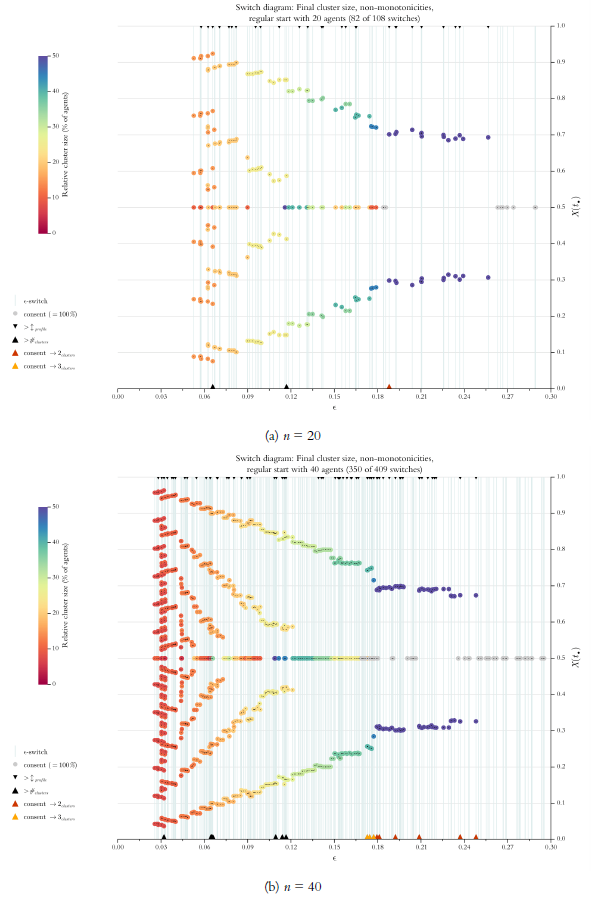
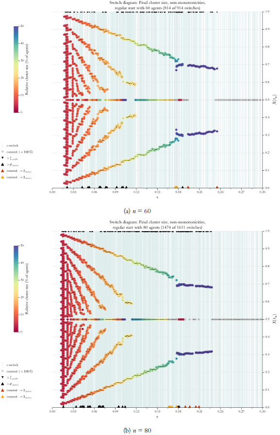
Understanding made easy: Switch by switch analysis of single runs
To answer such questions, we can exploit an advantage of our global approach: For all values of \(n\), and for each switch \(\epsilon^*\), there is a unique single run that produced the final stable structure that a switch diagram shows for \(\epsilon^*\). Thus, to find explanations, we can directly go into the details of the involved single runs—no statistics involved. And we can do that switch by switch: in their consecutive order, we follow our list of \(\epsilon\)-values that make a difference. Compared to the ‘traditional’ approach that compares single runs for which their \(\epsilon\)-value increases with a constant step size, the new approach has a major advantage: With the traditional approach it is a matter of luck that an \(\epsilon\)-value is also an \(\epsilon\)-switch. As a consequence, it may well be the case that consecutive \(\epsilon\)-values belong to the same segment, or, that there is no \(\epsilon\)-value that falls into an existing segment of the segmentation (understood in the sense of Equation 12). Central details are then missed or not visible in full precision.36
With a switch-by-switch approach it is different: We have the guarantee that we never miss an \(\epsilon\)-value that makes a difference, while, at the same time, we study only \(\epsilon\)-values that make a difference (for a BC-process with a given start distribution).
Here in this article we can illustrate this approach only by an example—doing it for all central findings is too much. We will focus on the wild transition from polarisation to consensus. Above, in Figure 11, we saw for \(n=42\) a very high number of switches (namely six), that destroy a consent by generating structures with three final clusters. The switch diagram in Figure 19a shows that the relevant switches are in the range between \(\approx 0.165\) and \(\approx 0.195\). Figure 19b is a switch diagram for that range only. Now details become visible that in Figure 19a are hidden by overlapping: Obviously, from left to right, the outer clusters become bigger and bigger, while the centre cluster, if it is not a consensus, becomes smaller and smaller. Additionally, now we can clearly see and distinguish the six switches that (though \(n\) is even!) turn a consent into a polarisation with two big outer clusters and one small centre cluster.
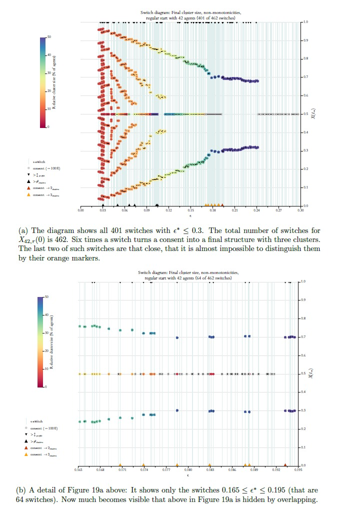
How comes? For an answer we exploit that we know perfectly well all the switches in the critical range of \(\epsilon\)-values. That allows to produce a sequence of unique single run visualisations of all possible BC-processes \(\langle X_{42,r}(0),\epsilon^* \rangle\) in that range. As a result we get this movie:
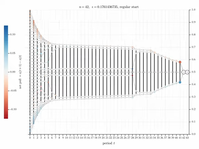
It is revealing and eye-opening to go switch by switch, back and forth, through the sequence of BC-processes, carefully studying the changes in the trajectories. As an example, here in this article, we will focus on a sequence of three consecutive switches that regard the first wild transition polarisation, consent, polarisation again. In the sequence, that are the pictures 8 to 10. Figure 21 shows a static version.
- In the first process (Figure 21a) until \(t=5\), all profiles \(X(t)\) are what we called \(\epsilon\)-profiles (cf. equation [ 8] ). But in \(t=6\) the profile splits twice. In \(t=8\) the process is stable. The final structure is a 3-cluster-structure with two outer clusters (17 agents each), and one centre cluster (8 agents).
- The next switch, which is only slightly larger (the difference is \(\approx 0.00131\))), changes the situation dramatically (see Figure 21b): The agent that moved upwards on a steep trajectory in Figure 21a and joins the upper cluster at \(t=7\) is still moving upwards, but the agent remains within the \(\epsilon\)-reach of the central cluster. As a bridge between the centre and the outer cluster, the agent prevents the network from falling apart. The same is true for its mirror agent in the lower half of the process. As the dark red color of the outer cluster at \(t=27\) (indirectly) indicates, the bridge is no longer necessary: From this time on, the outer cluster itself is within the \(\epsilon\)-reach of the centre. As a consequence, the bridge and the outer cluster merge at \(t=28\). In the next period, the two outer clusters come into mutual \(\epsilon\)-reach (again indirectly indicated by the dark red color). As a consequence we get consensus at \(t=30\) and stability in the next period.
- The next switch in Figure 21c is again only a tiny bit larger than its predecessor (the difference is \(\approx 0.00024\)). But again, the consequences are dramatic: The two agents that acted as bridges between the centre and the two outer clusters in Figure 21b start moving towards the emerging outer clusters at \(t=4\). Without bridges between the centre and the outer clusters, the profile splits at \(t=6\). The process ends as it ended under the first switch: A 3-cluster polarisation in the same period with the same size of all clusters. However, there is a difference to the first switch: Under the third switch, the width of the final stable profile is smaller (but the next switch will generate a non-monotonicity with respect to this; see Figure 19b).
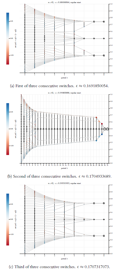
Obviously, in our example, the emerging or non-emerging of bridges between outer and central clusters plays the crucial role in the back and forth of consent and a 3-cluster polarisation. In the example given here, the bridges consist of just one agent that, for some periods \(t\), is critical: Without the agent the network would fall apart, while with the agent, in a slow process, an outer cluster is pulled direction center. If one goes switch by switch through the processes in the animation, it becomes clear that what one sees in this example also applies in general: Network bridges that emerge for certain switches, but—due to tiny changes in the local balance of upward or downward pulls—do not evolve for successor switches, are the decisive causes for the non-monotonicities with regard to the final cluster structure. The images of the BC-processes generated by the switch sequence also show that the bridges keeping the network together and, at the same time, contracting it, can have a more complicated structure than in Figure 21b. And the bridges work slowly: In one of these processes, it takes \(43\) periods to reach a stable consensus.37
This section has used BC-processes with the start distribution \(X_{42,r}(0)\) as an example of how to achieve an understanding of the processes through a switch-by-switch analysis. By its nature, this type of analysis can be applied to any start distribution and the finite set of BC-processes that it can initiate.
Conclusions and Concluding Remarks
The entire new analysis of the BC-model begins with a straightforward observation: A BC-process \(\langle X(0), \epsilon \rangle\) generates a sequence of network structures. An \(\epsilon^*\) > \(\epsilon\) can change these network structures as they evolve from one period to the next if and only if, for at least one agent, the set of \(\epsilon\)-insiders (and hence the complementary set of \(\epsilon\)-outsiders) changes in at least one period. The next larger \(\epsilon^*\) for which this is the case, is an \(\epsilon^*\) whose value equals the minimum distance to an \(\epsilon\)-outsider with regard to the entire process \(\langle X(0), \epsilon \rangle\). Formally, this is expressed as: \(\epsilon^* = \delta_{min}^{out} \bigl(X(0), \epsilon \bigr)\) (cf. Equation 11).
Such an \(\epsilon^*\) makes a difference, and we therefore called it an \(\epsilon\)-switch. This concept led to the possibility of using an algorithm to search step by step for all switches of a given start distribution, beginning with the smallest distance to an \(\epsilon\)-outsider in \(\langle X(0), \epsilon=0 \rangle\). This algorithm yielded a complete and finite list of all switches. From this list we obtain a complete segmentation of \([0, 1]\) into right-open intervals. In each segment, all \(\epsilon\)-values lead to the same BC-process.
In mathematical contexts, it is not uncommon to indirectly prove the existence of something without being able to explicitly present what has been proven to exist. Our approach stands in contrast to this: For any start distribution, we can effectively present all \(\epsilon\)-values that create a difference. That, then, made it possible to study all switches and their consequences, such as whether they generate particular non-monotonicities. The presentation of this approach used as an example a simple irregular start distribution. Subsequently, we conducted a systematic analysis of regular start distributions, wherein \(n\) agents are distributed equidistantly in the opinion space \([0, 1]\).38
The core findings of our new approach can be summarized as follows:
- Non-Monotonicity: BC-processes \(\langle X(0), \epsilon^* \rangle\) often result in non-monotonic changes within certain ranges of \(\epsilon\)-values. This manifests in several ways, such as:
- A consensus may be disrupted multiple times by subsequent switches.
- The number of final clusters and the final profile widths may increase with the next switch.
- Subsequent switches may lead to significantly longer stabilization times for the same initial distribution.
- Transition to Consensus: There is always an \(\epsilon\)-switch beyond which there is only consensus, or the final profile widths and stabilization times decrease monotonically. However, this transition is neither smooth nor gradual but rather wild and chaotic.
Why did we miss this in Hegselmann & Krause (2002)? That the BC-processes for a given start distribution depend on the confidence level \(\epsilon\), is trivial. But we did not even suspect that there could be a switch structure, already implicit in the start distribution, which divides the parameter space of \(\epsilon\) into finitely many segments within which the BC-processes are identical. Not suspecting this, it seemed reasonable, first, to increase \(\epsilon\) with constant step size (the step size was \(0.01\)), and, second, to compute for each step a certain number of BC-processes with random start distributions, and then, finally, to average over the number of final clusters (Hegselmann & Krause 2002 cf. 11ff. and 20ff.). In this averaging, the wildness and chaotic nature of the transition plurality \(\rightarrow\) polarization \(\rightarrow\) consensus then vanished.
However, we could have been warned: In our papers Hegselmann (2004) and Hegselmann & Krause (2005), one also finds the coefficients of variation (relative standard deviations) to the means for the respective \(\epsilon\)-values.39
In certain \(\epsilon\)-regions, namely those in which, as we know now, polarisation and consensus fluctuated, this coefficient spiked significantly. Such a pattern should have prompted further inquiry, yet we failed to recognize its significance at the time.40
In the analysis of BC-processes presented here, equidistant start distributions play an important role. Because it is probably the easiest to capture among the infinitely many equidistant start distributions, we have repeatedly used the so-called regular start distribution. It distributes \(n\) agents in the opinion space \([0, 1]\) (with the value \(0\) for the first, and the value \(1\) for the last agent). There is every reason to take the regular start distribution as the mother of all equidistant starting distributions: If one knows the properties of the mother (e.g., the number of switches) for a certain number \(n\) of agents, then one knows directly the properties of all equidistant starting distributions for the same \(n\); or else one can obtain these properties by very simple transformations (so with the exact position of the switches). This is then, of course, also true for a very special equidistant start distribution, which we have called expected value start distribution. It is a deterministic idealisation of infinitely many uniform random start distributions: In their ascending ordering, the \(i^{th}\) opinion is exactly there, where it will be at the average over infinitely repeated draws of \(n\) opinions that are uniformly distributed on the unit interval.
If, back in 2002, instead of a larger number of random start distributions with 625 agents each, we had simply used one and the same expected value start distribution with \(n = 50\), then some experimentation with the step size with which \(\epsilon\) increases, would have revealed dramatic and unmistakable non-monotonies: At a step size of \(0.01\), one would have seen the first non-monotonies only if one looked very closely; at a step size of \(0.0025\), the oscillation between consensus and dissent would have been strikingly evident.41 Even without the switch-concept, a subsequent inspection of the individual BC-processes for an increasing \(\epsilon\) (with constant step size) would have led to an early form of the type of analysis presented in Section 1.1.5.3. This would have made the importance of bridges between outer clusters and a cluster in the centre of the opinion space unmistakably clear.
The plea for single-run analyses in the style of Section 1.1.5.3 does not mean that, from now on, we should forget about iterated runs based upon random start distributions. Both approaches have complementary strengths and weaknesses: An analysis that always starts with the same expected value start distribution and then runs a switch by switch inspection of the generated processes, makes it easy to discover generic effects and to understand the mechanisms that produce them. At the same time, however, the approach blinds us to effects that are due to the fact that for random start distributions the distances of neighboring opinions are not equal to the expected value of this distance. And even more, the expected value approach can produce artifacts.42
Here is an example: For odd values of \(n\), in all BC-processes starting with an expected value distribution, under conditions of a homogeneous and constant \(\epsilon\), there is always a centrist opinion \(x = 0.5\) that never moves.43 Thus, in principle, the center can never be completely dissolved and torn apart (while at the same time, at least over a few periods and for some agents, there exists a force that pulls them direction center). This will be true in this form for practically no random starting distribution. As a heuristics, one is therefore well advised to use expected value start distributions with even values of \(n\): only they allow for a complete destruction of the center.44 Overall, it seems that we can say: Our old work in Hegselmann & Krause (2002) is an instructive example of how the study of BC-processes by an analysis of large numbers of random start distributions can easily obscure the view for crucial details. The best strategy seems to be to combine both the switch-based expected-value approach and the random approach.45
Our analysis of \(\epsilon\)-switches yields an interesting by-catch. It is related to the third option in dealing with the systemic inaccuracies of floating-point arithmetic: Stick to floating-point arithmetic, but, as a precaution, always add a tiny amount \(\Delta_\epsilon\) to \(\epsilon\) (cf. Section 1.1.3.2). That was meant to avoid missing an \(\epsilon\)-insider. We mentioned that, as a matter of fact, we had done so, successfully it seems, by always adding \(\Delta_\epsilon = 10^{-12}\). Now we are in a position to understand, first, why that normally works, and, second, why it was ex ante too risky for the switch analysis in this paper.
As we have seen, the switches for a start distribution \(X(0)\) lead to a complete segmentation of the unit interval into segments of right open intervals (cf. Equation 12). That the segments are right-open, has an important consequence: Whatever the value of \(\epsilon\), there is always some clearance for adding a tiny bit to \(\epsilon\) without changing the process. This effect is what we exploit with our correction mechanism. In Figure 3 we can see how and why it works: By adding \(\Delta_\epsilon = 10^{-12}\) to \(\epsilon\) we get the consequences of a representational floating-point error corrected, and the \(\epsilon\)-insider sets are now correct. But how do we know that our correction measure did not result in the complimentary error, namely taking an \(\epsilon\)-outsider as an insider? Well, from our perfect knowledge of all switches of the start profile \(X(0)\) in Figure 3, it is clear that all distances between consecutive switches are considerably larger than the \(\Delta_{\epsilon}\) added.46 These considerations yield a general lesson: As long as we add to \(\epsilon\) an \(\Delta_\epsilon\) that is smaller than the distance to the next switch, we can be sure not to mistake an \(\epsilon\)-outsider for an insider. Thus, if we had let our algorithm search switches using floating-point arithmetic, but doing that with our precautionary measure, this would have been numerically fine as long as no switches appeared whose distance was smaller than \(\Delta_\epsilon\).
Fortunately, about this matter we now know a lot: Figures 17 and 18 make it visually very clear that with an increasing \(n\), the density of switches increases dramatically. In Figure Figure 17b, in some regions the switches are that close to each other that it becomes difficult to even tell them apart. Luckily, when we compute the switches for a profile \(X_{n,r}(0)\), it takes only a few lines of code to compute the minimal distance between switches. In all the regular start distributions for the values \(n=2, 3, \dots, 50\), the minimal distance of two consecutive switches is \(3125/69117192732672 \approx 4.521306315328398 \times 10^{-11}\). That is still about 45 times larger than \(\Delta_\epsilon = 10^{-12}\). And that means: Yes, for \(n \leq 50\) we could have done our switch structure analysis of regular start distributions using floating-point arithmetic, if combined with our precaution measure—numerically, it would have worked.47 But we know that only ex post, namely after an analysis that used exact fractional arithmetic with integers of arbitrary length.
For \(n\)-values much bigger than 50, our precaution will not work any longer. There is probably some clearance for a refinement of our precaution: We could reduce our \(\Delta_\epsilon\) by some orders of magnitude. But with the increasingly dense distribution of switches, \(\Delta_\epsilon\) will have to become so small that it will no longer be large enough to prevent \(\epsilon\)-insiders from being mistaken as outsiders. Then we are left with exact fractional arithmetic—costly as it is in terms of computation time.
It is easy to underestimate the importance of integers of arbitrary length, but they are absolutely necessary. For example, among the switches for the start profile \(X_{36,r}(0)\) we find
| \[\epsilon_{250}^* = 16258104217541909608839193 \ / \ 96402696684456210048000000.\] | \[(14)\] |
The denominator of the fraction is about \(10^7\) times larger than the largest integer value that can be represented as a 64-bit integer. Converted into a 64-bit float, we get \(\epsilon_{250}^* = 0.16864781563899275\). For \(X_{36,r}(0)\) that is also the first switch that leads to a consent. For \(X_{47,r}(0)\) the first switch behind which all switches lead to consent, can no longer be displayed in one line of text (given our font size). The exact denominator of that switch (it is \(\epsilon_{417}^*\)) is
| \[1716162143883950154581321932800000000 \ (\approx 1.7 \times 10^{36}).\] | \[(15)\] |
The denominator is about \(1.8 \times 10^{17}\) times larger than the largest integer that can be represented in the 64-bit format. And the number is astronomical in a fairly literal sense—it corresponds to roughly half the estimated number of atoms in the universe.
There is a major issue in my analysis: For central claims and results, I basically have only computational evidence, but not the rigorous proofs. There are at least three analytical tasks:
- The algorithm that finds the switches always reached the largest switch (known in advance) and then stopped. So the list of switches was always finite. But for very large values of \(n\), e.g., \(5000\) agents, I did not even try to compute the switches, because already for higher two-digit values of \(n\), computation times in the range of one hour were needed.48
- If \(\epsilon^*\) is the \(\epsilon\)-switch of the process \(\langle X(0), \epsilon \rangle\), then, trivially, for \(\epsilon^*\)-values from the right-open interval \([\epsilon, \epsilon^*)\), the network structure (given by the sets of \(\epsilon^*\)-insiders) is unchanged. Thus, for \(\epsilon\)-values from this interval, the trajectories cannot change either. By definition, however, \(\epsilon^*\) then changes the network structure. Consistent computational evidence suggests that this always leads to some kind of change in the trajectories: If the switch \(\epsilon^*\) was found in period \(t\) of the process \(\langle X(0), \epsilon \rangle\), then trajectories of the process \(\langle X(0), \epsilon^* \rangle\) will be the same as those of the process \(\langle X(0), \epsilon \rangle\) up to period \(t\), but diverge thereafter.49
- In computational experiments with different equidistant start distributions that had the same number \(n\) of agents, all start distributions had the same total number of \(\epsilon\)-switches; switches with the same index, had the same number of final clusters, the same time to stabilisation, and were found in the same period \(t\). And more generally, all fundamental characteristics of BC-processes remain unchanged under positive-affine transformations of the start distribution. The initialisation may be equidistant or randomly generated. Its placement within the unit interval or somewhere else in the continuum of real numbers is irrelevant. The properties of the resulting BC-processes remain constant; only the switches require a transformation in the same manner. The geometric structure of the trajectories and the network structures indicated by the vertical lines remain constant, only varying in size.
In all three cases, it will be possible to provide rigorous proofs. However, I guess that the missing proofs will need to be found by someone else.
Finally, the question naturally arises as to the relevance of the results presented here. First of all, it should be noted that the wild, chaotic and non-monotonic behaviour of the BC-model only occurs over a limited range of \(\epsilon\)-values. On a larger scale, we have only studied equidistant start distributions here. For even and odd numbers of agents, the wild range of \(\epsilon\)-values is different in size: for even numbers, it is significantly larger. In both cases, however, the wild behaviour ceases to exist in the range \(\epsilon > \ \approx 0.35\). The results show that as \(\epsilon\) increases, there is a tendency towards Plurality \(\rightarrow\) Polarisation \(\rightarrow\) Consensus with respect to the stable final cluster structure. But it is only a tendency, not a monotonic transition. And the same applies to the final profile widths, the final number of clusters, and the stabilisation times.
Random start distributions were not studied at all in this article. Compared to equidistant start distributions, they naturally have many more of the switches that can be found at \(t=0\).50 It is certain that the non-montonic effects also occur with random start distributions. My few experiments so far with random start distributions also suggest that the wild behaviour of BC-processes occurs in a similar range of \(\epsilon\)-values as for equidistant distributions. However, how often non-monotonies occur will have to be determined by computational experiments. For example, one might assume that the symmetries of the forces pulling up or down due to the equidistant start favour the decay of consensuses under the next larger switch. With random start distributions, this type of non-monotonicity would become rarer. Other types may be more common.
In this context, the search for exotic initial distributions could become interesting: In the very many experiments with equidistant start distributions, I have never come across a start distribution for which there would have been an \(\epsilon\)-switch that would have led to a final cluster structure with more than three clusters after a consensus under its predecessor switch. In my relatively few experiments with random start distributions, I have never encountered the case where the next larger switch after a consensus leads to a final structure with three clusters. Do such cases not exist at all? If so, why not? And if they exist, why are they so rare?
In the BC-processes examined in this article, both \(\epsilon\)-insiders and \(\epsilon\)-outsiders are detected with impeccable precision, devoid of any calculation errors, no matter how minute (not even those permissible by today’s computing standards, such as the IEEE 754 standard). This level of accuracy surpasses human capabilities. Consequently, real-world BC-processes will invariably exhibit some level of noise (even if implemented in a normative-technical manner). This noise could profoundly impact BC-processes, potentially smoothing out non-monotonicities. However, to truly comprehend the ramifications of noise, it is essential to discern its effects on the intrinsic noise-free BC-processes. Understanding these processes is paramount—–and hopefully we now have achieved that.
Acknowledgements
In a certain sense, this article is the result of at least three decades of intensive discussions with Ulrich Krause. Without these discussions, this article would not exist.
Until I retired, I worked at the University of Bayreuth for almost two decades. As members of the Research Centre for Modelling and Simulation of Socio-economic Phenomena (MODUS) there, Jörg Rambau, Sascha Kurz, Torsten Eymann and I had a joint research seminar for many years. In was in this research seminar that the pitfalls of floating-point arithmetic dawned on me—albeit very slowly. The trick of adding a small \(\Delta\) to \(\epsilon\) to prevent \(\epsilon\)-insiders from being mistaken for \(\epsilon\)-outsiders, goes back to Jörg Rambau. Through discussions with Sascha Kurz I discovered that there is an exact arithmetic that can be used on a normal computer. It was in our joint seminar that the then still obscure idea arose that one should somehow be able to search specifically for those \(\epsilon\)-values that cause the wild transitions in the BC-processes. In 2014, I presented an early version of the \(\epsilon\)-switch diagrams in our seminar. The diagrams were still based on floating-point arithmetic and were therefore numerically vulnerable—they could not really be trusted. Igor Douven finally convinced me that I could solve all my problems using the newly developed programming language JULIA. In retrospect, I am very grateful to him for never giving up trying to convince me despite my stubborn resistance. And he always helped me patiently and immediately when I got stuck again in my early attempts to analyse the BC-model using JULIA programs.
I have presented the idea of an algorithmic search for \(\epsilon\)-switches in lectures at various places (Amsterdam, Bayreuth, Dresden, Palma de Mallorca, Regensburg, Utrecht, Zurich) in recent years. Many questions and comments from the different audiences have helped me to see and write more clearly. Igor Douven, Werner Raub and two anonymous reviewers have made very helpful suggestions to give this rather long text a hopefully readable structure.
Appendix A: Analytical Notes on central properties of \(\epsilon\)-switches
In this Appendix A we state explicitly some Analytical Notes. They are partially mathematical observations, important to note, but easy to prove. Some are short summaries or direct logical consequences of our definitions. Others are conjectures, suggested by experimental computations in exact arithmetic, possibly hard to prove. For ease of reference we number the Analytical Notes.
Analytical Note 1. A BC-process \(\langle X(0),\epsilon\rangle\) generates changing network structures that are given by the sets \(I\bigl(i,X(t), \epsilon \bigr)\), for all \(i \in I\) and \(t = 0, 1, \dots, \bar t\) (cf. Equation 2). For any BC-process \(\langle X(0),\epsilon\rangle\) with an \(\epsilon\) that is strictly smaller than the profile width of \(X(0)\),51 there exists a smallest \(\epsilon^* > \epsilon\) that changes somewhere the network structures. \(\epsilon^*\) equals the minimum distance to an \(\epsilon\)-outsider that can be found somewhere in the BC-process \(\langle X(0),\epsilon\rangle\). More precisely: \(\epsilon^* = \delta^{out}_{min}(X(0),\epsilon) = min{|x_i(t) - x_j(t)| for \, t = 0,1,\dots,\bar{t},\,i=1,\dots,n}\) and all \(j \in O\bigl(i,X(t), \epsilon \bigr)\}\). Such an \(\epsilon^*\) is called an \(\epsilon\)-switch.
Analytical Note 2. If \(\epsilon^*\) is a switch for the BC-process \(\langle X(0),\epsilon\rangle\), then at some point in time, at least two agents, that beforehand were \(\epsilon\)-outsiders become \(\epsilon\)-insiders. If \(\epsilon^*\) was found in period \(t\) of \(\langle X(0),\epsilon\rangle\), then the trajectories of the BC-processes \(\langle X(0),\epsilon\rangle\) and \(\langle X(0),\epsilon^*\rangle\) start to differ from \((t+1)\) onwards.
According to Analytical Note 1 and by definition, switches cause a change in the sets of \(\epsilon\)-insiders and \(\epsilon\)-outsiders. These sets characterise the network structure at time \(t\). Analytical Note 2 claims a corresponding change in the trajectories of the two processes \(\langle X(0),\epsilon\rangle\) and \(\langle X(0),\epsilon^*\rangle\): Given \(\epsilon^*\) is a switch for the BC-process \(\langle X(0),\epsilon\rangle\) that was found in period \(t\), the claim is that then
| \[\langle X(t+1),\epsilon\rangle \neq \langle X(t+1),\epsilon^*\rangle.\] | \[(16)\] |
In all our computations of switches we have checked whether or not that is the case. It always was the case. But why? So far, we do not have a proof.
Analytical Note 3. For any start distribution \(X(0)\), we can systematically search for \(\epsilon\)-switches. The first and smallest switch \(\epsilon_1^ *\) is the minimum distance between two opinions in \(X(0)\). Trivially, that minimum is a distance between neighboring opinions in the start profile; \(\epsilon_1^*\) changes in \(t=1\) the network structure of the BC-process \(\langle X(0),0 \rangle\).
Analytical Note 4. For any start distribution \(X(0)\), there is always a largest switch that somewhere changes the network structure, namely \(\epsilon^* = x_n(0) - x_1(0)\). No \(\epsilon\) value larger than that switch, can lead to different network structures. The largest switch is the last switch that the algorithm finds. Its value equals the width of the start profile.
Both the smallest and the largest switch can be directly found in the start profile \(X(0)\). We will call such switches primary \(\epsilon\)-switches. There are more. Upon reflection, all absolute distances \(|x_i(0) - x_j(0)|\) with \(i \not= j\), must necessarily be primary switches. Taking into account that \(|x_i(0)-x_j(0)|=|x_j(0)-x_i(0)|\), we get the maximum number of different distances by adding up the number of distances of agent\(_1\) to the agents with the indices \(2, \dots, n\) plus the number of distances of agent\(_2\) to the agents with the indices \(3, \dots, n\), and so forth, until we get to agent\(_n\) who has no distance to any agent with a higher index. Thus, the maximum number of different distances is
| \[ \sum_{i=1}^{n-1} i = \frac{n \ (n-1)}{2}.\] | \[(17)\] |
{#max_primary_switches} A strictly ordered start profile has also a certain minimum number of primary switches: In a strictly ordered profile, we have for sure the \((n-1)\) different distances of agent\(_1\) to the agents with the indices \(2, \dots, n\). If the start profile is equidistant in the sense that there is a constant \(c = x_{i+1}(0) - x_{i}(0)\) for \(i = 1, \dots, (n-1)\), then we will not find any additional different distance. Thus, the minimum number is simply \((n-1)\).
Analytical Note 5. A strictly ordered start profile \(X(0)\) with \(n\) opinions has at least \((n-1)\) and at most \(n(n-1) / 2\) primary switches. Start profiles with the minimum number of primary switches are equidistant. With an increasing \(n\), the minimum number of primary switches grows linearly, while the maximum number increases polynomially. Trivially, the number of primary switches is always finite.
Above in Section 1.1.4.1, in our example with \(n=5\), the maximum number of primary switches is therefore 10. Due to the special structure of our example in which several distances between opinions are the same, we have two primary switches less than in principal are possible.
Analytical Note 6. The search for switches can be done by the algorithm described in Figure 6. That algorithm came to an end and stopped whenever it was used. In other words: Whatever the start distribution \(X(0)\) that we searched for their switches, we always found a finite list of switches. As it seems, the number of switches of all start distributions is always finite.
What we here conjecture is by no means trivially so. Why is it that there are no regions in \([0, 1]\) with an infinite number of switches? So far, all algorithmic searches came to an end, and, thereby, stopped with a finite switch list. The largest switch was always the width of the start profile. That suggests that there is always a finite number of switches. But that is not a proof.
Analytical Note 7. The finite list of strictly increasing \(\epsilon\)-switches that the algorithm finds, gives a complete and exhaustive segmentation of \([0,1]\) by the following sequence of intervals (Equation 12 in the main text): \[% \langle \ [0,\epsilon_1^*)\ , \ [\epsilon_1^*,\epsilon_2^*)\ ,\ \dots, \ [\epsilon_{s-1}^*,\epsilon_s^*) \ , \ [\epsilon_s^*,1] \ \rangle \ \text{with} \ 0 < \epsilon_1^* < \epsilon_2^*,\ \dots,\ \epsilon_s^* \leq 1.\] The segments are right-open intervals except for the last one. For all \(\epsilon\)-values in the same segment, the whole process \(\langle X(0), \epsilon \rangle = X(0), X(1), \ \dots, \ X(\bar t)\) is always the same. The \(s\) processes \(\langle X(0), \epsilon_1^*\rangle, \dots, \ \langle X(0),\epsilon_s^*\rangle\) are all different. Together they exhaust all possible BC-processes with the start profile \(X(0)\).
There is a surprising by-catch of our approach: In the usual BC-process, \(j\)’s membership in \(i\)’s \(\epsilon\)-insider set at time \(t\), is defined by the condition that \(|x_{i}(t) - x_{j}(t)| \leq \epsilon\) (cf., Equation 2). But—under a robustness perspective—one might ask: What happens, if we modify the condition to \(|x_{i}(t) - x_{j}(t)| < \epsilon \,\)? For an answer we go back to our example start distribution \(X(0) = \langle 0, 0.18, 0.36, 0.68, 1.0 \rangle\). Our search algorithm finds as the first minimal \(\epsilon\)-outsider distance \(\delta_{min}^{out}=9/50\). In the modified process opinions exactly on the border are no insiders any longer. For all \(\epsilon\)-values up to and including \(9/50\), it holds that ‘nothing happens’; the process is stable in \(t=1\). Thus, the first segment of exactly the same processes is now the closed interval \([0, 9/50]\). The second segment in which all processes are the same, is now the left-open interval \((9/50,8/25]\). And so it goes on.
Analytical Note 8. If we modify the \(\epsilon\)-insider condition of Equation 2 of the original BC-process to \(|x_{i}(t) - x_{j}(t)| < \epsilon\), then we get again a complete and exhaustive segmentation of \([0,1]\) by the list of switches found by the algorithm. But now the sequence of intervals is left-open except for the first interval, namely \[ \langle \ [0,\epsilon_1^*]\ , \ (\epsilon_1^*,\epsilon_2^*]\ ,\ \dots, (\epsilon_{s-1}^*,\epsilon_s^*] \ , \ (\epsilon_s^*,1] \ \rangle \ \text{with} \ 0 < \epsilon_1^* < \epsilon_2^*,\ \dots,\ \epsilon_s^* \leq 1.\] Again, the segmentation exhausts all possibilities of the modified process.
Thus, what the modification does, is simply a ‘less than tiny’ right shift of the same sequence of dynamical patterns—a very strong robustness with regard to the modification. Note that the search algorithm described in Figure 6 does not need to be modified: The point is to find the distances to nearest \(\epsilon\)-outsiders. Once one knows for a certain process \(\langle X(0), \epsilon \rangle\) the distance \(\delta_{min}^{out}\), one knows the smallest larger \(\epsilon\)-value \(\epsilon^* = \delta_{min}^{out}\) that changes the sequence of network structures in such a way that at least one link is created that was not there before. From that fact we infer for the original BC-process that all processes in the segment that start with \(\epsilon^*\), are the same, while in the modified process the segment starts left-open to the right of \(\epsilon^*\).
Analytical Note 9. Let \(X(0) = x_{1}(0), \dots , x_{i}(0), \dots, x_{n}(0)\) be an arbitrary start distribution with the \(\epsilon\)-switches \[\epsilon_1^*, \dots, \epsilon_k^*, \dots, \epsilon_s^*,\] and let \(X^\diamond(0)\) be a start distribution obtained from \(X(0)\) by the positive-affine transformations \[x_i^\diamond(0) = \alpha \cdot x_i(0) + \beta \text{ with } \alpha > 0; \ \alpha, \beta \in \mathbf{R}; \text{ for } i=1,\dots, n.\] The \(\epsilon\)-switches of \(X^\diamond(0)\) are then simply multiplicative transformations of the \(s\) switches of \(X(0)\), namely \[\alpha \cdot \epsilon_1^*, \dots, \alpha \cdot \epsilon_k^*, \dots, \alpha \cdot \epsilon_s^*.\] For all switches of \(X^\diamond(0)\) holds: The \(k^{th}\) switch \(\alpha \cdot \epsilon_k^*\) of \(X^\diamond(0)\) has, apart from its transformed value, exactly the same properties as the \(k^{th}\) switch \(\epsilon_k^*\) of \(X(0)\).
According to Analytical Note 9, the properties of the \(\epsilon\)-switches of a start distribution \(X(0)\) remain unaffected by positive-affine transformations of the components of the start distribution. For instance, the stabilization times, final cluster structures, and all non-monotonicities remain the same. And the opinion space in which the BC-processes take place is irrelevant. It could be the unit interval or something different.
Appendix B: Universal Characteristics of Equidistant Start Distributions
A strictly ordered start distribution \(X(0)\) is equidistant (or equally spaced) if and only if
| \[ \big(x_{i+1}(0) - x_{i}(0) \big) = constant \ c, \text{ for } i = 1, \dots, \, (n-1).\] | \[(23)\] |
In the article, we encountered two different equidistant start profiles. The first was the regular start distribution according to Equation 9. That is a start profile of equally spaced opinions that starts with \(x_1(0)=0\) and ends (in the ascending order) with \(x_n(0)=1\). The second, the expected value start distribution according to Equation 10, is a very special, namely representative start profile: The \(i^{th}\) opinion is directly the average \(i^{th}\) opinion over infinitely repeated draws of \(n\) opinions that are uniformly distributed and then sorted in their ascending order. It is a kind of unique deterministic idealization of repeated draws of a uniform random distribution on the unit interval.52 Expected value start distributions are central for a very fruitful methodological approach: One relies on one and the same expected value start distribution (e.g., with \(n = 50\)). For that constant start distribution one analyses the effects of, for instance, stepwise increasing confidence levels \(\epsilon\). On purpose and programmatically, the approach deviates from the usual practice to run, firstly, a major number of random initialisations, and then, secondly, to do some statistics on the runs. Of course, the expected value approach blinds to effects that depend largely on the randomness of initialisations. But, the approach may, and often does, expose directly effects that are otherwise hidden and hard to detect in averages. Additionally, the approach easily reduces computation time by one to three orders of magnitude.53 Thus, the study of social processes that start with expected value start distributions is directly helpful with regard to questions which arise in the context of an empirical, analytically minded social science that aims at explanations of social phenomena. The approach sharpens the sense for unexpected phenomena and, at the same time, opens the eyes for possible explanations. Therefore, this type of start distribution is interesting for reasons far beyond a purely formal and purely mathematical interest.
However, all possible equidistant start distributions for a given \(n\) can be understood as positive-affine transformations of any of these start distributions. Therefore Analytical Note 9 (see Appendix A) implies that, for a given \(n\), we need to examine just one equidistant start distribution to know everything about any other equidistant start distribution with the same \(n\). Which one should we use? Is there one with a salient feature? To my mind, the regular start distribution has an advantage, namely the intuitiveness of the profile width of \(X(0)\): Whatever the value of \(n\), we know that in a regular start profile it always holds that \(x_1(0)=0\) and \(x_n(0)=1\). From a psychological point of view, this structure is the easiest to grasp (at least for me). For this very pragmatic reason, I often use the regular start distribution in the following as a kind of ‘mother of all equidistant start distributions’. By \(X_{r,n}(0)\) I refer to a regular start profile with \(n\) agents.
Analytical Note 10. All equidistant start distributions with \(n\) agents have the same number \(s\) of \(\epsilon\)-switches. Their respective lists of switches differ by a multiplicative transformation of all \(s\) switches by a factor \(\alpha\).
If \(c_{r,n}\) is the equidistance of a regular start profile with \(n\) agents and \(c_n\) the equidistance of any other equidistant start profile with \(n\) agents, then we get the list of \(\epsilon\)-switches of the latter by a multiplicative transformation of the regular switches by the factor \[\alpha = \frac{c_{r,n}}{c_n}.\]
If \(X_{n,r}(0)\) is a regular and \(X_n(0)\) is an expected value start distribution, then we get the list of \(\epsilon\)-switches of the latter by a multiplicative transformation of the regular switches by the factor \(\alpha = (n-1)/(n+1)\). \[\alpha = \frac{n-1}{n+1}.\]
The properties of the \(k^{th}\) of the \(s\) switches are always the same.
Analytical Note 11. For increasing even values of \(n\), and as well – but separately – for increasing odd values of \(n\), the number of switches increases monotonically. In both cases the increase is more than linear. It looks like a polynomial increase. In most cases, but not always, the number of switches for an odd \(n\), is greater than the number of switches for the even number \((n+1)\). See Figure 9.
Analytical Note 12. For even values of \(n\), often many switches exist that destroy a consent that their predecessor switch generated. As even values of \(n\) become larger, there seem to be larger numbers of such cases. For odd values of \(n\), there are no switches that destroy a consensus and, at the same time, lead to polarisation in the strict sense of just two final clusters. See Figure 10.
Analytical Note 13. There seem to be no switches that destroy their predecessor’s consent, and then lead to more than three final clusters.
We can look at switches that destroy consents under a more general perspective: Such switches generate a final cluster structure with more clusters than their predecessor does. But that may occur not only in the case of consent, i.e., a case with just one cluster. It may happen as well, that, instead of previously six, the next switch generates a final structure of seven (or more) clusters. And, indeed, that happens—even quite often. Figure 22 shows that this type of non-monotonicity occurs increasingly often. For \(n=46\) we get \(19\) such cases. By comparison of Figure 22 with Figures 10 and 11 one can easily verify that: From Figure 11 we know that for \(n=46\), in six cases a consent is turned into polarisation. From Figure 10 we know that for \(n=46\), in one case a consent switch is succeeded by a switch that generates three final clusters. Thus, in 12 of the 19 cases we get increasing numbers of clusters that are structurally different from ‘blowing up’ a consent.
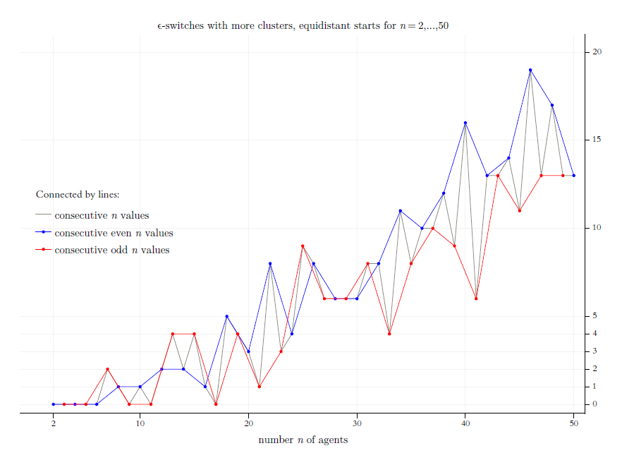
Analytical Note 14. For increasing even and odd values of \(n\), there is a non-monotonic tendency to occurrences of ever greater numbers of switches that, compared to their immediate predecessor, lead to more final clusters. In most, but not all cases, regular start distribution with an even value \(n\) have more such switches than the start distribution for the odd value \((n-1)\). See Figure 22.
In Figure 23 we focus on switches that – compared to their predecessor – let the final profile width increase. Trivially, that happens by all switches that ‘blow up’ a consent. But it also happens under other conditions. For \(n=50\) we have a total of \(607\) switches of an equidistant start profile. As we see in Figure 23, \(90\) of the switches generate an increasing final profile width.
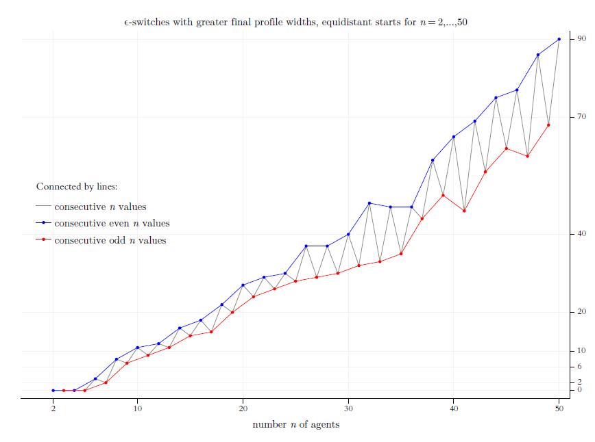
Analytical Note 15. For increasing even and odd values of \(n\), there is a non-monotonic tendency to ever greater numbers of switches that, compared to their immediate predecessor, lead to a larger final profile width. For an even value of \(n\), the number of such switches never seems to be smaller than their number for the odd value \((n-1)\). In most, but not all cases, a regular start distribution with an even value \(n\) have more such switches than the start distribution for the odd value \((n-1)\). The difference between the two numbers of switches seems to be increasing. See Figure 23.
The Figures 9 to 11, 22 and 23 show for regular start profiles \((n=2,3, \dots, 50)\) the number of their \(\epsilon\)-switches or frequency data on certain effects that they cause, for instance destroying a consent. The figures do not give information about the exact positions of the switches in the interval \([0,1]\) as Figures 12 does. Figures 24 to 26 have the same structure of the axes as in Figure 12: On the \(x\)-axis we have the complete range of possible \(\epsilon^*\)-values, i.e., \([0,1]\). The \(y\)-axis shows the increasing values of \(n\), i.e., the number of agents in a regular start profile \(X_{n,r}(0)\). As a consequence, each switch is a certain point \(\langle x,y \rangle\) in the coordinate system thus given. At this point we position a colored circle that indicates by its color the specific feature that we visualise by the diagram: Above in Figure 12, it was the final number of clusters; now, in Figure 24, it is the final profile width; in Figure 25, it is the time to stabilisation; and in Figure 26, it is the period in which the switch was found. The colormaps together with legends (both to the left) give the information how to read the specific diagram.
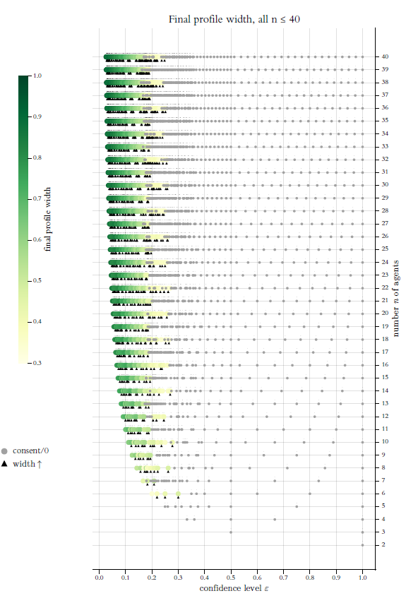
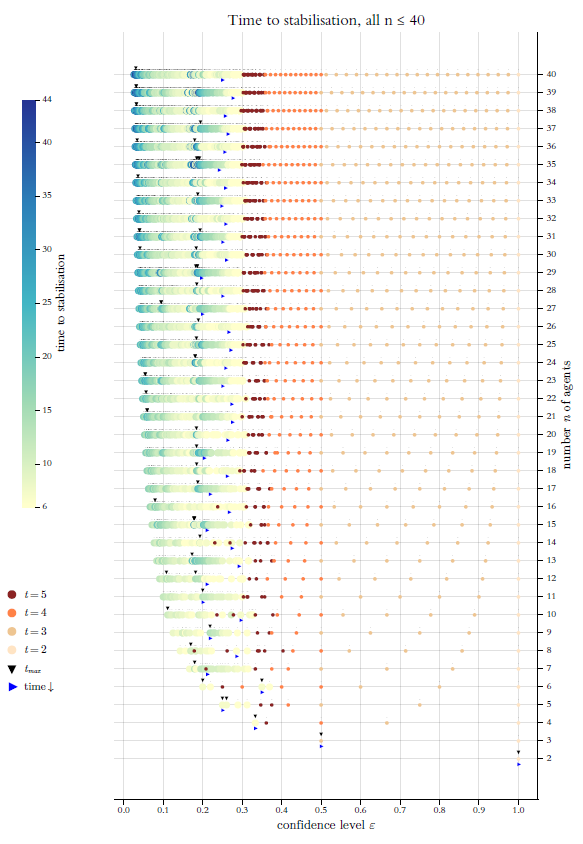
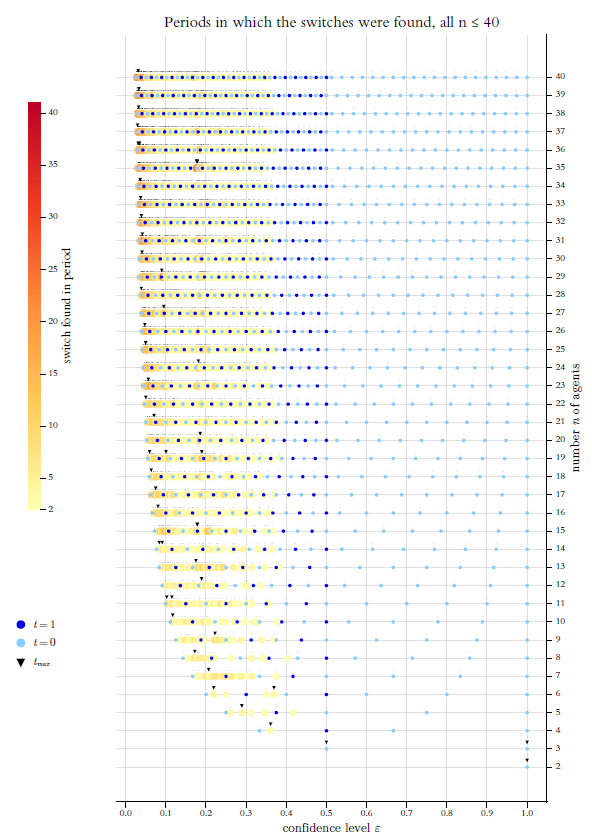
Figure 24 looks at the final profile widths. Trivially, a zero width means consent. Again, we mark specific non-monotonicities: Black triangles hint to switches that lead to a larger final profile width than the predecessor switch does.
The positional overview in Figure 25 focuses on the times to stabilisation. Short times get a special treatment: By four different reddish/brown colors we indicate stabilisation times \(t=2,3,4,5\). A downwards directed black triangles marks switches that, for the given value of \(n\), require the maximum time to stabilisation. A horizontally and rightwards directed blue triangle marks the switch from which onwards the stabilisation times decrease monotonously.
The final positional overview in Figure 26 shows each switch with the period in which it was found. \(t=0\) and \(t=1\) get a special treatment by two blueish colors. Primary switches (found in \(t=0\)) are light blue; switches colored dark blue were found in \(t=1\). In this Figure a downwards directed black triangle marks the maximum period in which a switch was found (for the given \(n\)).
Figures 12 and 24 to 26 reveal a lot. Below I collect the most important observations:
- For all \(n\), there is always a switch that leads to a consensus that is final in the sense: No successor switch destroys the consent. Careful visual inspection (with a focus on \(n \geq 5\)) shows a clear difference between even and odd values of \(n\): For odd values the final consensus switch comes for significantly smaller \(\epsilon\)-values. Evidence: Figure 12.54
- The transition from a final plurality (i.e., a major number) of clusters to a final consensus (just one cluster) is wild: Only for a few values of \(n\), the first consensus switch is also the final one. Normally, from switch to switch, many times the number of final clusters decreases and increases again. The most dramatic cases of this type are the many cases of a back-and-forth of consensus and dissent (the latter in the sense of polarisation or a final structure with three clusters). Evidence: Figure 12.
- In terms of the final number of clusters, we see a ‘smooth’ monotonic transition from a plurality to consensus only for the profiles \(X_{n,r}(0)\) with \(n= 2,3,4,5,6,9,11,17\). Evidence: Figure 12.
- \(X_{7,r}(0)\) is the first profile in which a consent is destroyed: There are two switches that, after a consent under their predecessors, lead to a final cluster structure with three clusters. Evidence: Figure 12.
- \(X_{8,r}(0)\) is the first profile with a switch that generates a final cluster structure with more clusters than the predecessor switch and where the predecessor did not lead to a consent. Evidence: Figure 12.
- \(X_{10,r}(0)\) is the first profile with a switch that destroys a consent and leads to polarisation in a strict sense. Evidence: Figure 12.
- \(X_{26,r}(0)\) is the first profile that has it both: four switches generate polarisation after a consent; one switch generates a final cluster structure with three clusters, while the predecessor switch leads to consensus. Evidence: Figure 12.
- An enormous number of switches leads to an increasing final profile width. We find this type of non-monotonicity for all start distributions with \(n\geq 6\), and they occur much more often than the non-monotonicities with regard to the final number of clusters. Evidence: Figures 24 and 12.
- There are very few cases of a monotonic decrease of the final profile width, namely just the profiles \(X_{n,r}(0)\) for \(n= 2,3,4\)—not even a handful. Evidence: Figure 24.
- The maximum stabilisation times tend to increase as \(n\) increases. For a given \(n\), the stabilisation times are radically non-monotonic for switches \(\epsilon^* < \, \approx 0.27\). Particularly long stabilisation times seem to concentrate in certain zones: A first zone in the region of very small \(\epsilon^*\)-values; a second zone exists for switches around \(\approx 0.2\). Evidence: Figure 25.
- For somewhat larger values of \(n\), switches that lead to a stabilisation in \(t=5\) are concentrated in the region from about \(0.3\) to about \(0.35\). Evidence: Figure 25.
- For \(\epsilon^* = 0.5\) (always a switch) it holds: Is \(n\) even, that switch leads to stabilisation in \(t=4\); is \(n\) odd, we always get stabilisation in \(t=3\). Evidence: Figure 25.
- Without exception, all switches strictly greater than \(0.5\) and strictly smaller than \(1\), lead to stabilisation in \(t=2\). The last switch always leads to stabilisation in \(t=1\). Evidence: Figure 25.
- For somewhat larger values of \(n\), the monotonic decrease of the times to stabilisation normally begins at \(\epsilon^*\)-values of about \(0.27\). But there are clear exceptions to this, namely the values \(n=12, 15, 17, 19, 27, 29\). Evidence: Figure 25.
- For switch values smaller than about \(0.3\), the periods in which the switches are found, are clearly non-monotonically distributed. Evidence: Figure 26.
- The positions of the primary switches (by definition found in \(t=0\)) and as well the switches found in \(t=1\), clearly follow a regular pattern. For primary switches that is no surprise; for the switches found in \(t=1\) it is. For both types, the distance between two consecutive occurrences of them is always the equidistance of the start profile. All positions of primary switches are multiples of the respective equidistance of their start distributions. Evidence: Figure 26 together with a computational check.
- With the exception of \(n=5\) and \(n=8\), for all \(n\), all switches \(\epsilon^* \geq 0.4\) are found in \(t=0\) or \(t=1\). Evidence: Figure 26.
- For \(\epsilon^* = 0.5\) (always a switch) it holds: Is \(n\) even, that switch is found in \(t=1\); is \(n\) odd, the switch is found in \(t=0\) (primary switch). Evidence: Figure 26.
- Without exception, all switches strictly greater than \(0.5\) are found in \(t=0\) (primary switches). Evidence: Figure 26.
Analytical Note 16. As a consequence and application of Analytical Notes 9 and 10, the findings from Figure 12and Figures 24 to 26 hold correspondingly for all equidistant start distributions.
Appendix C: What (Not Only, But Especially) BC-Modellers Should Know About Floating-Point Arithmetic
Floating-point arithmetic is the type of arithmetic that computers today normally use for all their computations. Partially, that arithmetic is built into the hardware (FPU, the floating-point unit, supported by IUs, the integer units). Floating point arithmetic follows a certain standard, called IEEE 754 (named after the working group p754 of the Institute for Electrical and Electronics Engineers). The standard evolved over some decades since the 1950s, but was worked out in detail, and then published only in 1985; a major update and extension followed in 2008. Some details are tricky, but there is no mystery.55
Floating point-arithmetic is an arithmetic that operates on floating-point numbers (floats, for short). Floats are ‘engineered’ numbers in order to, firstly, approximate a very large range of the continuum of real numbers by a huge, but finite subset of real numbers, and then, secondly, to do numerical computing with them. One can engineer floats for any positional number system, whatever the base, but most important are the floats with base \(2\). They are the floats with which numerical computing normally is done.56 Such binary floats are represented in a sign-exponent-significand format by a fixed number of bits. Our computations used floats with a total of 64 bits to represent a number. It is a binary exponential representation by a bit string with a well defined structure: The string starts with 1 bit for the sign, then follow 11 bits for the exponent, and thereafter 52 bits for the significand (often called mantissa). The IEEE standard refers to these numbers as numbers of the type double precision. There are other types as well. Single precision has a total of 32 bits, single extended 40, and double extended 80. Since the 2008 update, IEEE 754 covers even 128 bit floats (quadruple precision).
Whatever their type, the representation of floats is normalised with regard to a standard position of the binary point. From the decimal scientific notation we know that there are equivalent ways to express a number in an exponential form: \(0.00036525\) could be written as \(0.36525 \times 10^{-3}\), but as well as \(3.6525 \times 10^{-4}\). Or, in other words, one can ‘float’ the decimal point to any position by repeatedly multiplying or dividing by 10, and decrementing or incrementing the exponent accordingly. In the binary system it is the same. In a normalised floating-point number, the position of the binary point is (except for zero, which is treated as an exception) always after the first nonzero bit in the binary expansion.57 Given this first convention58, it is not necessary to explicitly use the first bit of the significand to store the binary 1, each significand is simply considered as being implicitly preceded by a hidden 1, which gives one additional bit to increase precision.59 The number of bits of the exponent field determines the maximum number of different bit strings in that field. Given the 11 bits in the exponent field of double precision-floats, there are \(2^{11}=2048\) different bit strings. Following a second convention (called biased exponent), almost all of them are used to represent exponents in the range \(-1022\) to \(+1023\). The negative exponents allow an easy representation of very small absolute values of both positive and negative numbers.60 Additionally, a complication that is caused by the first convention, is fixed via the exponent field: The number zero can’t be represented as a normalised float with a hidden leading \(1\) of the significand, since an all zero significand is 1.0, not 0.0. The problem is solved by an explicit exception: As a third convention, an all zero exponent field \((00000000000)_2\), followed by an all zero significant field, signals zero. That, then, gives a possibility to represent numbers that are even smaller than the smallest normalised number, the so called subnormal (or denormalised) floats, which smooth the gap between zero and the smallest normalised float: As the number zero, they are characterised by an all zero exponent, but then followed by a significand bit string that is not all zero. For them, by a fourth convention, the leading hidden bit of the significand is set to 0, while the exponent is set to the smallest value (\(-1022\) for double precision). As a consequence, compared to normalised floats, the accuracy of subnormal floats drops sharply. Finally, by a fifth convention, the exponent field is used to introduce some useful special cases: The bit string \((11111111111)_2\) signals \(\pm \infty\) or NaN (not a number), depending upon whether or not the bit string in the significand field is all zero or not. These strange ‘numbers’ are introduced to manage numerical situations that traditionally were beyond repair, and often caused the computation to stop immediately, as for instance range overflows, underflows, or a division by zero.61 The elements of the set of real numbers that, along these lines, can be exactly represented, that are floats in a technically precise sense.
All the details of the representation (and that are far more than the five conventions that I use here for a short summary), plus exactness requirements on some elementary numerical operations with such numbers, plus requirements on format conversions (e.g., conversion of floats to an integer format), that is what the standard IEEE 754 specifies.
Not only in our context one should be aware of some important features of floats, and the arithmetical operations with them. I focus on 64-bits floats (1 sign bit, 11 exponent bits, 52 significand bits, i.e., the type double precision), since they are used in my computations. I look especially on floats from and in the ‘numerical world’ of all BC-processes, namely the unit interval. My main concerns are the magnitudes of the absolute errors (representational or operational), that we have to expect.
- For double precision the largest positive number is \(\approx 2^{1024} \approx 1.8 \times 10^{308}\). The smallest normalised positive float is \(2^{-1022} \approx 2.2 \times 10^{-308}\); the smallest subnormal float is \(2^{-52} \times 2^{-1022} \approx 4.9 \times 10^{-324}\). The range of negative floats has the analogous limits.
- If we think of the continuum of real numbers as a line, then floats are a finite number of points on that line, and they have a spacing. Floats are not uniformly distributed over their whole range. Close to zero they are densest. The spacing of floats follows perfect powers of \(2\): Within the left-closed and right-open interval between two consecutive perfect powers of \(2\), the floats are uniformly spaced. The total number of floats in each such interval is always the same, and this number is directly determined by the number of bits for the significand. Single precision leads to \(2^{23}= 8 388 608 \approx 8.4 \times 10^{6}\), double precision to \(2^{52}= 4503599627370496 \approx 4.5 \times 10^{15}\) floats in each interval. Since the size of the interval between two consecutive perfect powers of \(2\) always doubles, the gaps between the floats in consecutive intervals double as well. As a consequence, between \(2^{52}\) and \(2^{53} \ (\approx 9.0 \times 10^{15})\) double precision floats represent just the integers; above \(2^{53}\), not even all integers between consecutive powers can be represented.
- As a surprising consequence of the general principles, the situation in the unit interval \([0,1]\) is very special: In the upper half we have for \([0.5,1)\) what we always have between consecutive perfect powers of \(2\) (here the powers \(-1\) and \(0\)), namely \(2^{52} \approx 4.5 \times 10^{15}\) floats. For floats in the lower half of the unit interval, we have all the \(1022\) exponents \(\leq -1\). That gives us there \(1022 \times 2^{52} = 4602678819172646912 \approx 4.6 \times 10^{18}\) floats. By comparison, the interval \([1,2)\) contains only \(\frac{1}{1023}\) of the total number of floats in \([0,1)\). All the floats in \([1,2)\) are uniformly spaced with a perfect mirror symmetry with regard to \(1.5\), while in the unit interval we have 1023 different sizes of gaps between floats.62 About a half of all positive floats, lie in the interval \([0,1]\) (correspondingly, about a half of all floats lie in between \(-1\) and \(+1\)).
- Since almost all of the real numbers can not be represented, rounding is unavoidable. A non-representable real number will be rounded to the nearest representable float.63 Given double precision-floats with their 52-bits significand, we know that between two consecutive perfect powers of \(2\), there are always \(2^{52}\) equally spaced floats. Therefore, the nearest upper float of \(1\) is \((1 + 2^{-52})\). The distance between \(1\) and its nearest upper float, is called the machine epsilon; for double precision-floats it is \(machine_{\epsilon} = 2^{-52} \approx 2.2 \times 10^{-16}\). For any number \(x\) with \(1 < x < (1 + 2^{-52})\), the difference between \(x\) and its floating-point representation, is at most \(\frac{1}{2} \cdot machine_\epsilon = 2^{-53} \approx 1.1 \times 10^{-16}\). This value is an upper bound to the absolute error of rounding to the nearest representable float for real numbers \(x\) inbetween \(1\) and \((1 + machine_{\epsilon})\).64 But, because of the equal spacing of floats between consecutive perfect powers of \(2\), the same holds obviously for all real numbers in the interval \([2^0, 2^1)\). For real numbers in \([2^1, 2^2)\), the maximum absolute error doubles, in \([2^2, 2^3)\) it doubles again, and so forth. In the opposite direction, for negative exponents of \(2\), i.e., within the unit interval, the maximum absolute errors get smaller and smaller: In the upper half of the unit interval, i.e., in \([2^{-1}, 2^0)\), we have as many equally spaced floats as in \([2^0, 2^1)\), what halfs the gaps, and that halfs the maximum absolute rounding error. As a consequence, in the upper half of the unit interval, the maximum absolute error is \(\frac{1}{4} \cdot machine_\epsilon = 2^{-54} \approx 5.5 \times 10^{-17}\). In the lower half of the unit interval, following the decreasing perfect powers of \(2\), the stepwise halving of the maximum representational error continues.65
- Irrational or binary periodic numbers can never be exactly represented by the finite number of bits for their binary representation in the sign-exponent-significand format. They will be rounded to the nearest representable float. Increasing the number of bits for the binary representation increases precision, but can not solve the basic problem.
- Irrationality of numbers is invariant with regard to the base of a positional number system. But periodicity is not: A non-periodic number in the decimal system, may be periodic in the binary system. For ‘decimal natives’ it comes as a surprise that of all the ‘innocent’ numbers \(0.1, 0.2, \dots, 0.9\), it is only \(0.5\) that is binary non-periodic. Only 3 out of the \(99\) numbers \(0.01, 0.02, \dots, 0.99\) are binary not periodic, namely \(0.25, 0.50\), and \(0.75\). Just 7 out of the 999 numbers \(0.001, 0.002, \dots, 0.999\) are binary non-periodic, and, therefore, do not need a rounding to fit into the sign-exponent-significand format with a fixed finite number of bits.
- IEEE 754 sets and guarantees a certain exactness standard for some elementary arithmetical operations: For addition, subtraction, multiplication, and division, the fundamental requirement is: applied to any two floats \(x\) and \(y\), the result has to be equal to the rounded exact result. Additionally required are exactly rounded square roots and remainders. Though it is a surprisingly complicated task, meeting these requirements is possible, and even guaranteed. However, IEEE 754 only narrows down, but does not exclude operational errors. Some of them can easily be detected. An example is the subtraction \(1.0 - 0.68\) (one of the distances in our example start profile). We get \(0.31999999999999995\) as the result (as the absolute distance between the two involved numbers, we get the same result). Logically equivalent ways to calculate a value may lead to different results, the usual laws of commutativity and associativity do not apply in full generality, suddenly ‘superfluous’ parentheses matter. Example: For the division \(3 / 5\) we get the result \(0.6\), but for the equivalent calculation \(3 \cdot (1 / (4 + 1))\) we get \(0.6000000000000001\) (while, without the outer brackets in the latter expression, the computer gets it right). Here it is an operational error of the magnitude \(10^{-17}\), what is as well the magnitude of the maximum absolute representational error in the upper half of the unit interval. But in general, one has to know: Under the standard IEEE 754, there is no guarantee that the result of a sequence of elementary arithmetic operations is still the rounded value of the exact result. Often it is not. If an algorithm involves the sequential and iterated execution of arithmetical operations of all sorts, it may be a hard task, if not impossible, to determine how accurate one’s computations with floats of a certain type can be expected to be.
Notes
For the history of the BC model and its systematic classification in the broader field of related or alternative modelling of opinion dynamics, see sections 1-3 of Hegselmann & Krause (2002). For a more recent overarching classification and generalisation to high dimensional opinion spaces see the book (Hegselmann & Krause 2019; Krause 2015).↩︎
For a detailed and careful comparison of the HK- and the DW-model see Urbig et al. (2008).↩︎
For overviews on models of opinion dynamics, differences and relationships between them, see Lorenz (2007), Xia et al. (2011), Sı̂rbu et al. (2017), Flache et al. (2017), Proskurnikov & Tempo (2017), Proskurnikov & Tempo (2018), Noorazar (2020), Noorazar et al. (2020), Bernardo et al. (2024).↩︎
Lorenz (2006) inspired the more rigorous mathematical analyses in Wedin (2021), Wedin (2022). The non-monotonic decrease in the number of stable clusters is also noted and highlighted in Proskurnikov & Tempo (2018 p. 7f. and Table 1) and Srivastava et al. (2023 p. 588f. and Fig. 2).↩︎
At this point, it is possible to individualise the confidence level by introducing agent-specific \(\epsilon_i\)-values. However, since this type of heterogeneity does not play a role in the following and would only complicate the notation, I will not do so.↩︎
If the boundaries of the confidence interval are outside the unit interval \([0,1]\), then the confidence interval is empty in these areas since a BC-process can never lead to opinions outside \([0,1]\). It is therefore not necessary to exclude confidence intervals that are too wide.↩︎
The number \(n\) of agents is implicitly given by the number of components of \(X(0)\).↩︎
This is not necessarily so. In principle, the same formalism could be applied to interacting atoms or molecules, where Equation 4 is concerned with changes in some physical property. For the view that models consist of a formalism and an interpretation see as a classical reference Gibbard & Varian (1978).↩︎
But note that a BC-process, applied to such opinions, makes sense only under the condition of intersubjective comparability of intensities.↩︎
There are now hundreds of books and thousands of articles on mechanisms and effects of social media. Revealing analyses are, for example, Pariser (2011) and Sunstein (2018); both books received a very wide attention and response. In recent years, numerous attempts have been made to better understand the effects and mechanisms of social media through modeling and simulation; cf. the highly instructive overview of Flache et al. (2017). The works of Keijzer et al. (2018), Keijzer & Mäs (2021), Marijn A. Keijzer & Mäs (2022), and Marijn A. Keijzer (2022) are very thoughtful and successful examples of such efforts. They also contain very informative overview sections.↩︎
For a concise description of Carnap’s work see Leitgeb & Carus (2023).↩︎
For a very detailed and comprehensive analysis of Carnap’s understanding of explication, its development and its embedding in current discussions in philosophy of science, see the article of Brun (2016); see as well section 1.1 and the supplement “D. Methodology” in Leitgeb & Carus (2023).↩︎
For these problems cf. Roscher et al. (2020).↩︎
In philosophy of science, a lively discussion has developed in the last 15 years about what understanding actually is, or what could be meant by the term; cf. on this Grimm et al. (2016), Baumberger & Brun (2016), De Regt (2017). Of particular interest is the connection between understanding and having explanations. Previously, the discussion in philosophy of science had concentrated only on the concept of explanation; for a summary see Salmon (2006).↩︎
For this approach see Mäki (1992), Mäki (2011). Helpful and clarifying in this context are the analyses of ceteris absentibus, ceteris neglectis, and ceteris paribus conditions in Boumans & Morgan (2001).↩︎
This view on opinion formation models is similar to the one Rodrik (2015) takes with regard to models in economics:
...simple models of the type that economists construct are absolutely essential to understanding the working of society. Their simplicitiy, formalism, and neglect of many facets of the real world are precisely what make them valuable. They are a feature, not a bug. What makes a model useful is that it captures an aspect of reality. What makes it indispensable is that it captures the most relevant aspect of reality in a given context. Different contexts—different markets, social settings, countries, time periods, and so on—require different models. And this is where economists typically get into trouble. They often discard their professions’s most valuable contribution—the multiplicity of models tailored to a variety of settings—in favor of the search for the one and only universal model (Rodrik 2015 p. 11).
Rodrik believes that attempts to develop an all-encompassing large-scale model are misguided. He writes:
...efforts to construct large-scale economic models have been singularly unproductive to date. To put it even more strongly, I cannot think of an important economic insight that has come out of such models (Rodrik 2015 p. 39).
For a discussion and (partial) critique of Rodrik from a philosophy of science perspective, see Mäki (2018).↩︎
Winkler’s central focus is on subjective probability distributions with unknown parameters, but not on point probabilities.↩︎
Cf. the very first motivating introduction of the BC-model in Krause (1997 p. 47ff.), Krause (2000 sec. 1), and Hegselmann & Krause (2002 sec. 1 and 2).↩︎
The first Delphi study concerned a secret US Air Force project on the question of an optimal selection of industrial American targets from the point of view of a Soviet strategic planner, in order to reduce munitions production by a given percentage. In particular, the number of atomic bombs required was to be estimated (cf. Dalkey & Helmer 1963 p. 458). For security reasons, this new study format was not reported for the first time until ten years later. For the subsequent development and use of the Delphi format over the last 60 years, see Khodyakov et al. (2023).↩︎
DeGroot (1974) is entitled Reaching a Consensus. In his Conclusions, DeGroot explicitly discusses the relationship of the DG-processes to the abstract communication structure of the Delphi format. He explicitly points out that the DG-mechanism—unlike the Delphi format—does require knowledge of the identity of the others because of the assignment of weights \(w_{ij}\). This is not necessary for BC-processes. One only needs to know the opinions of the others.↩︎
See Lehrer (1975), Lehrer (1976), Wagner (1978), Lehrer & Wagner (1981). It is noteworthy that Lehrer and Wagner do not conceive of the DG-process as an exchange process that takes place in time, but rather as an iteration process that is started after the end of the discussion process and that can also be left to a machine. Their starting point is a “dialectical equilibrium” i.e., a situation after “the group has engaged in extended discussion of the issue so that all empirical data and theoretical ratiocination has been communicated. ... the discussion has sufficiently exhausted the scientific information available so that further discussion would not change the opinion of any member of the group” (Lehrer & Wagner 1981 p. 19). The multiplication of a weight matrix with a column of probabilities is then iterated. Under relatively weak requirements for the entries in the weight matrix, this leads to consensual weights for \(t \rightarrow \infty\) and a corresponding consensual probability estimate (cf. Lehrer & Wagner 1981 p. 21ff.).↩︎
In a series of articles Igor Douven, together with different coauthors, has used the BC-model to find efficient epistemic policies for groups that encounter certain research problems, e.g., finding the probability \(p\) of a Bernoulli process, or the best explanation for a given explanandum; cf. I. Douven & Riegler (2010), I. Douven (2010), Douven & Kelp (2011), Douven & Wenmackers (2017) and Douven & Hegselmann (2022). The articles draw on the extended BC-model as it was published in Hegselmann & Krause (2006), Hegselmann & Krause (2009); see also the discussion in R. Hegselmann & Krause (2015 sec. 6). The extended BC-model is explicitly meant to capture, in a formalised and stylised way, a fundamental truth about human learning, namely, that it is an interplay of learning from others and learning from the world. In Hegselmann & Krause (2006), Hegselmann & Krause (2009) all the details of the learning from the world were put into a black box. The articles of Douven et al. demonstrate that the black box can be opened. See also Douven & Hegselmann (2021). For a strictly technical application, see also R. Hegselmann et al. (2015).↩︎
As to the position of the \(y\)-axis’ ticks and labels on the right side of the coordinate system, I follow the data presentation style of the Economist.↩︎
After the initial subtraction error, NETLOGO produces different versions of the dynamics thereafter, though there isn’t any random component in the definition of the dynamics. However, if one keeps the seed for the random generator constant, one always gets the same miscalculations. The strange effect is probably due to some internal randomness as to the sequence in which the additions are done, together with the fact that the usual laws of commutativity and associativity do not hold in full generality in the floating-point arithmetic. As a consequence, results become numerically path dependent.↩︎
The articles Polhill & Izquierdo (2005), Polhill et al. (2006) , Izquierdo & Polhill (2006) are an extremely helpful series of articles on floating-point arithmetic in general and all the sorts of damages that it can cause especially in agent-based models.↩︎
BC-processes are numerically vulnerable also in other respects. Here two other examples: We use the standard definition of stability, namely \(X(t-1)=X(t)\). But the floating point arithmetic almost always detects by far too late that in a BC-process two profiles are equal. That happens even in perfectly clear cases of a consent that is reached since some periods. A second example is the detection of clusters. In our context, it is very natural to consider as a cluster sets of agents with exactly the same opinion. But the floating-point arithmetic will detect’ tiny differences (again \(10^{-17}\) is the order of magnitude) where there are no differences under exact computation. In both cases, often visual inspection together with a little numerical reflection is completely sufficient to see that the computer gets it wrong. With regard to both stability checks and cluster identification it helps to introduce a tiny tolerance for being equal.↩︎
A different and more precise symmetry check is the following: In an equidistant start profile (regular or expected value), each agent \(i\) has a mirror agent \(j\) with the index \(j = n - (i-1)\). Both have exactly the same absolute distance to \(0.5\). For any pair \(i\) and \(j\) of mirror agents, in a numerically correct computation it holds at any time \(t\): The set of mirror agents of the elements in \(i\)’s insider set, equals the set of \(j\)’s insider set et vice versa. This type of mirror symmetry of insider sets of mirror agents can be checked and visualised.↩︎
Both the working and the limitations of the trick based upon certain choices of \(\Delta_\epsilon\) can be studied by systematic symmetry checks as described in footnote 28.↩︎
Soon it will become clear that this seemingly ‘innocent’ start distribution generates surprising non-monotonicity effects. The start distribution was originally found by Malte Sieveking in a general analytical way and then adapted to the framework with opinion values in the unit interval. Malte Sieveking and Ulrich Krause intend to present a type of analysis that is different from mine. I will come back to their approach later in footnote 38.↩︎
See in Appendix A Analytical Note 10↩︎
Wedin & Hegarty (2015) use equidistant start distributions with an equidistance \(c = 1\).↩︎
In Figure 12, it is always the first consensus-switch (grey circle) after the last non-monotonicity marker that leads to the first consensus that is not destroyed any more.↩︎
Lorenz (2006) [5.4; cf. his figures \(10\), \(11\) and \(13\)] calls this type of diagrams bifurcation diagrams, following a terminology that is often used in dynamical systems theory. As he frankly states, his use of floating-point arithmetic causes asymmetries in his diagrams that do not exist for theoretical reasons [cf. ibid. 5.7]; cf. in this context our detailed discussion of symmetry problems in Section 1.1.3.1 above. The problems are exactly the ones that we illustrated by our Figure 4. Note also that, if the computations are done by floating-point arithmetic, symmetry does not guarantee numerical correctness—the errors could have been made in a symmetrical way. Symmetry is only a necessary, but not a sufficient condition for numerical correctness. Since Figure 13 top in Lorenz (2006) can’t be numerically correct, it is almost certain that Figure 13 bottom (the figure shows the convergence time) is not correct as well; it is just that one cannot detect the numerical incorrectness in this diagram by visual inspection. Since they are based upon exact arithmetic, all that will never happen with \(\epsilon\)-switch diagrams. The main structural difference between \(\epsilon\)-switch diagrams and the bifurcation diagrams in Lorenz (2006) is the following: \(\epsilon\)-switch diagrams show the cluster structure for all and only the \(\epsilon\)-values that really make a difference. If, on the other hand, the \(\epsilon\)-values on the \(x\)-axis increase with a constant step size, then it is a matter of luck that an \(\epsilon\)-value is also an \(\epsilon\)-switch. As a consequence, it may well be the case, that consecutive \(\epsilon\)-values belong to the same segment, or, that there is no \(\epsilon\)-value that falls into an existing segment of the segmentation (understood in the sense of Equation 12). Central details are then missed or not visible in full precision. Basically the same applies to the numerical approach to get Figure 2 in Srivastava et al. (2023). The authors describe clearly the numerical problems and then use a fixed precision for all their computations. However, this does not lead to correct calculations, but at best to the fact that calculation errors, such as those shown above in Figure 4, are no longer noticeable because they occur themselves symmetrically.↩︎
See footnote 34.↩︎
The articles Hegselmann & Krause (2015) and Hegselmann (2020) examine the role of network bridges in the context of radicalisation processes. Both articles were written without an understanding of the role of \(\epsilon\)-switches. It was shown that there are wild regions in the parameter space where very small differences in the initial conditions (be it the confidence level \(\epsilon\) or the number of radicals) lead to certain bridge structures emerging or not—with massively different consequences for the overall radicalisation effects that occur. These older analyses could become much more precise if they were based on the complete list of the \(\epsilon\)-switches specific to the respective dynamics.↩︎
In my approach, I first identify all \(\epsilon\)-values that make a difference at all. Only after that those switches are filtered out which destroy a consensus. Ulrich Krause and Malte Sieveking, on the other hand, are looking for a direct way to characterise those \(\epsilon\)-values that destroy consents. They will give a mathematical (topological) analysis in a forthcoming paper Consensus may be destroyed by increasing confidence: Phase transitions in the BC-model. Cf. footnote 30.↩︎
See in Hegselmann (2004 p. 24), Figure 3a and 3b. See in Hegselmann & Krause (2005), page 392, Figure 4 and then on page 393 Figure 5; in both figures look at the graphics top left for the arithmetic mean.↩︎
Very aptly, Wedin and Hegarty write about the BC-model: “The update rule ... is certainly simple to formulate, though the simplicity is deceptive” (Wedin & Hegarty 2015). At the time, the update rule in Equation 4 deceived me as well.↩︎
See the Figures 9.2 and 9.3 in Hegselmann (2020).↩︎
The artifact is structurally similar to the artifact studied in Hegselmann (1996 p. 222ff.). There an even or odd length of a \(2\)-dimensional cellular automata matters for the evolution of cooperation.↩︎
Cf. our discussion in Section 1.1.3.1. There we used that fact to identify BC-processes that are corrupted by numerical errors of the floating-point arithmetic.↩︎
Another problem, which I cannot discuss here, concerns the magnitude of \(n\). It must not be too small, because, as we have seen above, expected value start distributions for quite small \(n\)-values, have very special features. On the other hand, \(n\) should not be too large, because then one would not be able to see any details in the visualisation of the individual processes. I suspect that an \(n\) between \(50\) and \(100\) is a good choice for most purposes.↩︎
To some degree that is done in Hegselmann (2020 p. 224ff.).↩︎
We know by the search algorithm that the next larger \(\epsilon\)-switch is \(79/360\). All BC-processes with an \(\epsilon\)-value from the right-open interval \([1/5, 79/360)\) are the same. Thus, with \(\epsilon =1/5 + 10^{-12}\) we are clearly in the same segment, far distant from the (open) right border of the segment. As a consequence, we can definitely exclude that we mistook an outsider as an insider.↩︎
At the same time, we can exclude that \(\Delta_\epsilon = 10^{-12}\) is too small: What we are adding is several orders of magnitude larger than the representational and operational errors that we can expect under our conditions; see Appendix C on floating-point arithmetic.↩︎
However, my JULIA program is certainly far from minimizing computation times. For example, I did not use one of the great strengths of JULIA at all, namely the simple possibilities for parallelisation. But the search for switches can be parallelised: For a given start distribution \(X(0)\), the available processors could search for switches in parallel in specific sections of \([0,1]\). We get the final switch list by merging the partial results. This kind of parallelisation is possible because for the computing of \(\epsilon^*\) as the \(\epsilon\)-switch of the process \(\langle X(0), \epsilon \rangle\), one does not need to know the value of the predecessor switch of \(\epsilon^*\)—one simply searches from the given \(\epsilon\) to the right.↩︎
That the interplay of the trajectories and the changing network structures is key for an understanding of BC-processes is clearly seen in Wedin & Hegarty (2015). They write:
Associated to a given configuration ... of opinions is a receptivity graph \(G\) ..., whose nodes are the \(N\) agents and where an edge is placed between agents \(i\) and \(j\) whenever ... they interact with one another. The transition in the configuration from time \(t\) to time \(t + 1\) is determined by this graph at time \(t\). However, it is clear ... that the dynamics will affect the graph, which in turn affects the dynamics. This feedback is the basic reason why many beautiful conjectures about the HK-model remain unresolved ... (Wedin & Hegarty 2015 p. 2416).
And that is also the reason why above in Section 2.2, we directly introduced methods to visualise the dual nature of BC-processes as dynamical systems and dynamical networks.↩︎
Cf. Appendix A, the comments on Analytical Notes 3 and 4.↩︎
The proviso excludes that \(\epsilon\) itself is already the largest switch; cf. below Analytical Note 4.↩︎
We can do the same with regard to other types of random distributions. However, one has to derive the equations that then correspond to Equation 10. The equidistance in Equation 10 is due to the uniform random distribution. If, for example, we do the same with a normal distribution, the corresponding expected value distribution would not be equidistant. The relevant discipline here is order statistics; for an overview see David & Nagaraja (2003).↩︎
That is my experience. My interest in expected value start distributions originated in problems with computing time. Fruitful applications of the expected value approach can be found in Hegselmann & Krause (2015) and Hegselmann (2020).↩︎
In Figure 12, it is always the first consensus-switch (grey circle) after the last non-monotonicity marker that leads to the first consensus that is not destroyed any more.↩︎
The following description is for the most part based upon two excellent introductions into floating point arithmetic, namely Overton (2001) and Goldberg (1991).
Overton (2001) is Michael L. Overton’s 100-pages book Numerical Computing with IEEE Floating Point Arithmetic. On the cover, it additionally says Including One Theorem, One Rule of Thumb, and One Hundred and One Exercises. My appendix follows the chapters 2 and 3 in Overtone’s book. In a remarkable way, the book also covers the history and pre-history of the IEEE 754 standard.
Goldberg (1991) is David Goldberg’s long article (43 pages) What Every Computer Scientist Should Know About Floating-Point Arithmetic. For the title of my Appendix C I have stolen parts of Goldberg’s title.↩︎
Since 2008, IEEE 754 sets also the standards for floats with the base 10.↩︎
A general alternative to a floating-point representation is a fixed point representation: after the sign bit, one has a certain fixed number of bits for the representation of the number before the binary point; then follow the bits for the representation of the number after the binary point. Compared to a floating-point representation, the fixed point representation reduces the range of storable numbers severely.↩︎
“First convention” is my language, not the language in which the standard IEEE 754 originally was formulated. The same holds for the four other conventions that follow.↩︎
Because of the hidden leading bit 1, one can look at the significand as the fractional part of the mantissa. That is, why the significant is often simply called fraction.↩︎
The cost is that the largest representable number is only about half of what the largest in principle could have been, namely \(\approx 2^{2048}\).↩︎
For instance, under the IEEE 754 standard, \(0/0\) has a result, namely NaN (Goldberg 1991).↩︎
The huge number of different gaps contribute decisively to the many asymmetries in Figure 4. One might therefore have the idea of moving the BC processes into the interval \([1,2]\) (or further to the right) for the calculations, and then transferring the results of the calculation back to \([0,1]\) by subtraction. In essence, however, this is window dressing: the numerical errors are made more difficult to detect, but not eliminated. Cf. footnote 34 above.↩︎
There are three other modes of rounding: up, down, and towards zero. Here and in the following, I focus only on rounding to the nearest representable float.↩︎
Some authors refer to this value as the machine epsilon. As it seems, in computer and computational science the machine epsilon is normally the distance between \(1\) and the nearest upper float. Any confusion with our confidence level \(\epsilon\), \(\epsilon\)-switches, \(\epsilon\)-segmentation etc. has to be avoided.↩︎
Therefore, we can consider the \(machine_\epsilon\) as a way to measure the relative rounding error of a number \(x\). This error depends only upon the number of bits for the significand, while the absolute rounding error depends upon the size of \(x\).↩︎
References
ABELSON, R. P. (1964). Mathematical models of the distribution of attitudes under controversy. In N. Frederiksen & H. Gulliksen (Eds.), Contributions to Mathematical Psychology (pp. 142–160). New York, NY: Holt, Rinehart; Winston, Inc.
BAUMBERGER, C., & Brun, G. (2016). Dimensions of objectual understanding. In S. R. Grimm, C. BAUMBERGER, & S. Ammon (Eds.), Explaining Understanding: New Perspectives From Epistemology and Philosophy of Science (pp. 165–189). New York, NY: Routledge.
BERNARDO, C., Altafini, C., Proskurnikov, A. & Vasca, F. (2024). Bounded confidence opinion dynamics: A survey. Automatica, 159, 111302. [doi:10.1016/j.automatica.2023.111302]
BOUMANS, M., & Morgan, M. S. (2001). Ceteris paribus conditions: Materiality and the application of economic theories. Journal of Economic Methodology, 8(1), 11–26. [doi:10.1080/13501780010022794]
BRUN, G. (2016). Explication as a method of conceptual re-engineering. Erkenntnis, 81(6), 1211–1241. [doi:10.1007/s10670-015-9791-5]
CARNAP, R. (1950). Logical Foundations of Probability. Chicago, IL: University of Chicago Press.
DALKEY, N., & Helmer, O. (1963). An experimental application of the Delphi method to the use of experts. Management Science, 9(3), 458–467. [doi:10.1287/mnsc.9.3.458]
DAVID, H. A., & Nagaraja, H. N. (2003). Order Statistics. New Jersey: John Wiley & Sons.
DEFFUANT, G., Neau, D., Amblard, F., & Weisbuch, G. (2000). Mixing beliefs among interacting agents. Advances in Complex Systems, 3(01n04), 87–98. [doi:10.1142/s0219525900000078]
DEGROOT, M. H. (1974). Reaching a consensus. Journal of the American Statistical Association, 69(345), 118–121. [doi:10.1080/01621459.1974.10480137]
DE Regt, H. W. (2017). Understanding Scientific Understanding. Oxford: Oxford University Press.
DOUVEN, I. (2010). Simulating peer disagreements. Studies in History and Philosophy of Science Part A, 41(2), 148–157. [doi:10.1016/j.shpsa.2010.03.010]
DOUVEN, I., & Hegselmann, R. (2021). Mis- and disinformation in a bounded confidence model. Artificial Intelligence, 291(103415), 1–27. https://doi.org/https://doi.org/10.1016/j.artint.2020.103415 [doi:10.1016/j.artint.2020.103415]
DOUVEN, I., & Hegselmann, R. (2022). Network effects in a bounded confidence model. Studies in History and Philosophy of Science, 94, 56–71. [doi:10.1016/j.shpsa.2022.05.002]
DOUVEN, I., & Kelp, C. (2011). Truth approximation, social epistemology, and opinion dynamics. Erkenntnis, 75, 271–283. [doi:10.1007/s10670-011-9295-x]
DOUVEN, I., & Riegler, A. (2010). Extending the Hegselmann-Krause model I. Logic Journal of the IGPL, 18(2), 323–335. [doi:10.1093/jigpal/jzp059]
DOUVEN, I., & Wenmackers, S. (2017). Inference to the best explanation versus Bayes’s rule in a social setting. The British Journal for the Philosophy of Science, 68(2), 535–570. [doi:10.1093/bjps/axv025]
FLACHE, A., Mäs, M., Feliciani, T., Chattoe-Brown, E., Deffuant, G., Huet, S., & Lorenz, J. (2017). Models of social influence: Towards the next frontiers. Journal of Artificial Societies and Social Simulation, 20(4), 2. [doi:10.18564/jasss.3521]
FRENCH Jr, J. R. P. (1956). A formal theory of social power. Psychological Review, 63(3), 181–194. [doi:10.1037/h0046123]
GIBBARD, A., & Varian, H. R. (1978). Economic models. The Journal of Philosophy, 75(11), 664–677. [doi:10.5840/jphil1978751111]
GOLDBERG, D. (1991). What every computer scientist should know about floating-point arithmetic. ACM Computing Surveys (CSUR), 23(1), 5–48. [doi:10.1145/103162.103163]
GRIMM, S. R., Baumberger, C., & Ammon, S. (2016). Explaining Understanding: New Perspectives From Epistemology and Philosophy of Science. New York, NY: Routledge.
HARARY, F. (1959). A criterion for unanimity in French’s theory of social power. In D. Cartwright (Ed.), Studies in Social Power (pp. 168–182). Ann Arbor, MI: University of Michigan.
HEGSELMANN, R. (1996). Cellular automata in the social sciences: Perspectives, restrictions, and artefacts. In R. HEGSELMANN, U. Mueller, & K. G. Troitzsch (Eds.), Modelling and Simulation in the Social Sciences From the Philosophy of Science Point of View (pp. 209–233). Dordrecht: Kluwer Academic Publishers. [doi:10.1007/978-94-015-8686-3_12]
HEGSELMANN, R. (2004). Opinion dynamics: Insights by radically simplifying models. In D. Gillies (Ed.), Laws and Models in Science (pp. 19–46). London: King’s College Publications.
HEGSELMANN, R. (2020). Polarization and radicalization in the bounded confidence model: A computer-aided speculation. In V. Buskens, R. Corten, & C. C. P. Snijders (Eds.), Advances in the Sociology of Trust and Cooperation: Theory, Experiment, and Field Studies (pp. 197–226). Berlin: de Gruyter. [doi:10.1515/9783110647495-009]
HEGSELMANN, R., König, S., Kurz, S., Niemann, C., & Rambau, J. (2015). Optimal opinion control: The campaign problem. Journal of Artificial Societies and Social Simulation, 18(3), 18. [doi:10.18564/jasss.2847]
HEGSELMANN, R., & Krause, U. (2002). Opinion dynamics and bounded confidence: Models, analysis and simulation. Journal of Artificial Societies and Social Simulation, 5(3), 2.
HEGSELMANN, R., & Krause, U. (2005). Opinion dynamics driven by various ways of averaging. Computational Economics, 25, 381–405. [doi:10.1007/s10614-005-6296-3]
HEGSELMANN, R., & Krause, U. (2006). Truth and cognitive division of labour: First steps towards a computer aided social epistemology. Journal of Artificial Societies and Social Simulation, 9(3), 10.
HEGSELMANN, R., & Krause, U. (2009). Deliberative exchange, truth, and cognitive division of labour: A low-Resolution modeling approach. Episteme, 6(2), 130–144. [doi:10.3366/e1742360009000604]
HEGSELMANN, R., & Krause, U. (2015). Opinion dynamics under the influence of radical groups, charismatic leaders, and other constant signals: A simple unifying model. Networks and Heterogeneous Media, 10(3), 477–509. [doi:10.3934/nhm.2015.10.477]
HEGSELMANN, R., & Krause, U. (2019). Consensus and fragmentation of opinions with a focus on bounded confidence. The American Mathematical Monthly, 126(8), 700–716. [doi:10.1080/00029890.2019.1626685]
IZQUIERDO, L. R., & Polhill, J. G. (2006). Is your model susceptible to floating-Point errors? Journal of Artificial Societies and Social Simulation, 9(4), 4.
KEIJZER, M. A. (2022). Opinion dynamics in online social media. University of Groningen, PhD Thesis.
KEIJZER, M. A., & Mäs, M. (2021). The strength of weak bots. Online Social Networks and Media, 21, 1–12. [doi:10.1016/j.osnem.2020.100106]
KEIJZER, M. A., & Mäs, M. (2022). The complex link between filter bubbles and opinion polarization. Data Science, 5(2), 139–166. [doi:10.3233/ds-220054]
KEIJZER, M. A., Mäs, M., & Flache, A. (2018). Communication in online social networks fosters cultural isolation. Complexity, 2018, 1–18. [doi:10.1155/2018/9502872]
KHODYAKOV, D., Grant, S., Kroger, J., Gadwah-Meaden, C., Motala, A., & Larkin, J. (2023). Disciplinary trends in the use of the Delphi method: A bibliometric analysis. PLoS One, 18(8), 1–11. [doi:10.1371/journal.pone.0289009]
KRAUSE, U. (1997). Soziale Dynamiken mit vielen Interakteuren. Eine Problemskizze. In U. Krause & M. Stöckler (Eds.), Modellierung Und Simulation Von Dynamiken Mit Vielen Interagierenden Akteuren (pp. 37–51). Bremen: Universität Bremen.
KRAUSE, U. (2000). A discrete nonlinear and non-autonomous model of consensus. In S. N. Elaydi, G. Ladas, J. Popenda, & J. Rakowski (Eds.), Communications in Difference Equations: Proceedings of the Fourth International Conference on Difference Equations (pp. 227–236). CRC Press; Poznan: Gordon & Breach Science Publisher.
KRAUSE, U. (2015). Positive Dynamical Systems in Discrete Time. Berlin: de Gruyter.
LEHRER, K. (1975). Social consensus and rational agnoiology. Synthese, 31(1), 141–160. [doi:10.1007/bf00869475]
LEHRER, K. (1976). When rational disagreement is impossible. Noûs, 10(3), 327–332. [doi:10.2307/2214612]
LEHRER, K., & Wagner, C. G. (1981). Rational Consensus in Science and Society: A Philosophical and Mathematical Study. Berlin Heidelberg: Springer.
LEITGEB, H., & Carus, A. (2023). Rudolf Carnap. The Stanford Encyclopedia of Philosophy. Available at: https://plato.stanford.edu/archives/sum2023/entries/carnap/
LORENZ, J. (2006). Consensus strikes back in the Hegselmann-Krause model of continuous opinion dynamics under bounded confidence. Journal of Artificial Societies and Social Simulation, 9(1), 8.
LORENZ, J. (2007). Continuous opinion dynamics under bounded confidence: A survey. International Journal of Modern Physics, 18(12), 1819–1838. [doi:10.1142/s0129183107011789]
MAGEE, B. (1982). Men of Ideas: Some Creators of Contemporary Philosophy. Oxford: Oxford University Press
MÄKI, U. (1992). On the method of isolation in economics. In C. Dilworth (Ed.), Idealization IV: Intelligibility in Science (pp. 319–354). New York, NY: Rodopi.
MÄKI, U. (2011). Models and the locus of their truth. Synthese, 180(1), 47–63.
MÄKI, U. (2018). Rights and wrongs of economic modelling: Refining Rodrik. Journal of Economic Methodology, 25(3), 218–236.
NOORAZAR, H. (2020). Recent advances in opinion propagation dynamics: A 2020 survey. The European Physical Journal Plus, 135, 1–20. [doi:10.1140/epjp/s13360-020-00541-2]
NOORAZAR, H., Vixie, K. R., Talebanpour, A., & Hu, Y. (2020). From classical to modern opinion dynamics. International Journal of Modern Physics C, 31(07), 2050101. [doi:10.1142/s0129183120501016]
OVERTON, M. L. (2001). Numerical Computing With IEEE Floating Point Arithmetic. Philadelphia, PA: SIAM.
PARISER, E. (2011). The Filter Bubble: What the Internet Is Hiding From You. London: Penguin UK.
POLHILL, J. G., Izquierdo, L. R., & Gotts, N. M. (2006). What every agent-based modeller should know about floating point arithmetic. Environmental Modelling & Software, 21(3), 283–309. [doi:10.1016/j.envsoft.2004.10.011]
POLHILL, J. G., & Izquierdo, N. M., Luis R.and Gotts. (2005). The ghost in the model (and other effects of floating point arithmetic). Journal of Artificial Societies and Social Simulation, 8(1), 5.
PROSKURNIKOV, A. V., & Tempo, R. (2017). A tutorial on modeling and analysis of dynamic social networks. Part I. Annual Reviews in Control, 43, 65–79. [doi:10.1016/j.arcontrol.2017.03.002]
PROSKURNIKOV, A. V., & Tempo, R. (2018). A tutorial on modeling and analysis of dynamic social networks. Part II. Annual Reviews in Control, 45, 166–190. [doi:10.1016/j.arcontrol.2018.03.005]
RODRIK, D. (2015). Economics Rules: Why Economics Works, When It Fails and How to Tell the Difference. Oxford: Oxford University Press.
ROSCHER, R., Bohn, B., Duarte, M. F., & Garcke, J. (2020). Explainable machine learning for scientific insights and discoveries. IEEE Access, 8, 42200–42216. [doi:10.1109/access.2020.2976199]
SALMON, W. C. (2006). Four Decades of Scientific Explanation. Pittsburgh, PA: University of Pittsburgh Press.
SÎRBU, A., Loreto, V., Servedio, V. D. P., & Tria, F. (2017). Opinion dynamics: Models, extensions and external effects. In V. Loreto, M. Haklay, A. Hotho, V. D. P. Servedio, G. Stumme, J. Theunis, & F. Tria (Eds.), Participatory Sensing, Opinions and Collective Awareness (pp. 363–401). Berlin Heidelberg: Springer.
SRIVASTAVA, T., Bernardo, C., Altafini, C., & Vasca, F. (2023). Analyzing the effects of confidence thresholds on opinion clustering in homogeneous Hegselmann-Krause models. 31st Mediterranean Conference on Control and Automation (MED), IEEE [doi:10.1109/med59994.2023.10185838]
SUNSTEIN, C. (2018). # Republic: Divided Democracy in the Age of Social Media. Princeton, NJ: Princeton University Press.
URBIG, D., Lorenz, J., & Herzberg, H. (2008). Opinion dynamics: The effect of the number of peers met at once. Journal of Artificial Societies and Social Simulation, 11(2), 4.
WAGNER, C. (1978). Consensus through respect: A model of rational group decision-making. Philosophical Studies: An International Journal for Philosophy in the Analytic Tradition, 34(4), 335–349. [doi:10.1007/bf00364701]
WEDIN, E. (2021). A rigorous formulation of and partial results on Lorenz’s “consensus strikes back” phenomenon for the Hegselmann-Krause model
WEDIN, E. (2022). On the mathematics of the one-dimensional Hegselmann-Krause model
WEDIN, E., & Hegarty, P. (2015). The Hegselmann-Krause dynamics for the continuous-agent model and a regular opinion function do not always lead to consensus. IEEE Transactions on Automatic Control, 60(9), 2416–2421. [doi:10.1109/tac.2015.2396643]
WINKLER, R. L. (1968). The consensus of subjective probability distributions. Management Science, 15(2), 61–75. [doi:10.1287/mnsc.15.2.b61]
XIA, H., Wang, H., & Xuan, Z. (2011). Opinion dynamics: A multidisciplinary review and perspective on future research. International Journal of Knowledge and Systems Science (IJKSS), 2(4), 72–91. [doi:10.4018/jkss.2011100106]