Opinion Dynamics Model Revealing Yet Undetected Cognitive Biases

Université Clermont-Auvergne, Inrae, UR LISC, France
Journal of Artificial
Societies and Social Simulation 26 (4) 12
<https://www.jasss.org/26/4/12.html>
DOI: 10.18564/jasss.5196
Received: 06-Mar-2023 Accepted: 06-Sep-2023 Published: 31-Oct-2023
Abstract
This paper synthesises a recent research that includes opinion dynamics models and experiments suggested by the model results. The mathematical analysis establishes that the model's emergent behaviours derives from cognitive biases that should appear in quite general conditions. Moreover, it seems that psychologists have not yet detected these biases. The experimental side of the research therefore includes specifically designed experiments that detect these biases in human subjects. The paper discusses the role of the model in this case, which is revealing phenomena that are almost impossible to observe without its simulations.Introduction
In the chapter of their review devoted to opinion dynamics, Castellano et al. (2009) present a gallery of models: voter model (Ben-Naim et al. 1996; Sood & Redner 2005), majority rule model (Galam 2002; Krapivsky & Redner 2003), Sznajd model (Sznajd-Weron 2002), bounded confidence models (Deffuant et al. 2000; Hegselmann & Krause 2002), Axelrod model (Axelrod 1997; Klemm et al. 2003), CODA model (Martins 2008). The review enumerates the results of systematic simulations and theoretical approaches, generally inspired by statistical physics, explaining the patterns observed in these simulations. By contrast, model fitting or deriving from empirical data occupy a tiny part of the chapter, though Catellano et al. underline its interest and importance. In a more recent review about opinion dynamics, Flache et al. (2017) also describe a series of models, for instance models with negative influence (Huet & Deffuant 2010; Jager & Amblard 2005; Mäs et al. 2010) or argument based models (Mäs & Flache 2013) and also point out that few of them aim at reproducing empirically observed patterns of opinion distributions.
The trend in opinion dynamics research seems therefore very robust. Despite regularly announced good intentions to connect models more closely to empirical data, the core of the research activity remains inventing new models or better understanding the patterns produced by old ones. These models themselves attract interest when their dynamics relies on simple, reasonably justifiable, assumptions about opinion influence and when the simulations produce patterns that are difficult or sometimes almost impossible to predict from the mere knowledge of the interaction functions. In this case, understanding the process of pattern emergence becomes a research question in itself and often a challenging one, which triggers the motivation of researchers.
We agree that the research about fitting models on data or deriving models from data poses interesting challenges (Deffuant et al. 2008; Deffuant et al., 2022a) and that he field should invest more efforts on them. However, we think important to value inventing and studying various theoretical models as well. Indeed, this line of research produces new knowledge about possible complex phenomena that could not be conceived without a deep understanding of pattern emergence. We think that each of these models provides specific conceptual tools that may help perceive different facets of social complexity. In our view, the value of these achievements should clearly be recognised.
Moreover, we would like to underline a potentiality offered by theoretical models which is rarely considered. A theoretical model may suggest the existence of phenomena that are ignored in social sciences and that can only be detected by new specific experiments. In this case, the model is similar to a theory in physics predicting for instance the existence of a certain type of yet unknown particle, that is then experimentally confirmed. This paper precisely aims at reporting an example of such a model revealing a yet unknown social phenomenon that is then confirmed experimentally.
The model involves agents holding evaluations (called opinions in the original papers) about each other that evolve through noisy pair interactions (Deffuant et al. 2018; Deffuant & Roubin 2022). The simulations show rather unexpected emergent properties, which could be understood only with non-obvious approximations of average dynamics of the opinions. Moreover, the analysis of this approximate model reveals the crucial influence of two emerging biases: a positive bias on self-evaluations and a negative bias on the evaluations of others. The effect of these biases is quite small at each interaction, but the simulations suggest that it can add-up and become very significant over time.
Moreover, the mechanisms inducing the biases, as revealed by the model, seem yet unknown in social sciences. In particular, psychologists identify a well-known positive bias in self-evaluation, but its mechanism is very different. Thus the next arising question is: can the bias revealed by the model be observed in experiments with human subjects? Indeed, mathematically, the bias derives directly from general hypotheses relating influence and self-evaluation that seem reasonable.
In order to check these hypotheses, we designed an online questionnaire that was filled by 1500 participants (Deffuant et al., 2022b). The participants perform a simple task and then receive evaluations of their performance and are asked to self-evaluate in reaction to these feedbacks. The results confirm the hypothesis made in the model and the existence of the corresponding positive bias on self-evaluation.
This paper summarises the presentation of both the model and the experiment (their details can be found in the specific papers) with the aim to highlight the connection between them and illustrate a general approach that could be followed by others.
The rest of the paper is organised as follows. In the next section, we describe the opinion dynamics model and we explain how biases in the evaluations are responsible for the emerging patterns. Then, we focus on the positive bias in self-evaluation. We define it mathematically in a simplified case and describe the experiment that confirms its existence. Finally, we discuss the whole approach in a broader perspective.
The Model Revealing Biases
This section summarises the paper that describes the model and its patterns in details (Deffuant & Roubin 2022). The considered model is a simplified version of an earlier model (Deffuant et al. 2013). The original papers are in the field of opinion dynamics and the term "opinion" is used while "attitude" or "evaluation" would be preferred by psychologists or social-psychologists. In this paper, the experimental part refers mainly to the literature in social sciences and uses the term "evaluation" coming from this field. We also used this term instead of "opinion" in the description of the model in order to be consistent.
State and dynamics
The model includes \(N_a\) agents. Each agent \(i \in \{1,\dots, N_a\}\) holds an evaluation \(a_{ij}\) of each agent \(j \in \{1,\dots, N_a\}\) including themselves. The evaluations are real values between -1 and +1. In most simulations, at the initialisation, all evaluations are set to 0: agents have a neutral evaluation of themselves and of all the others at the beginning of the simulations.
Graphically, the agents’ evaluations can be represented as a matrix (see examples on Figure 1) in which row \(i\), with \(1 \leq i \leq N_a\), represents the array of \(N_a\) evaluations of agents \(j\) by agent \(i\). Column \(j\), with \(1 \leq j \leq N_a\), represents the evaluations of \(j\) by agents \(i\). Positive evaluations are represented with red shades and negative evaluations with blue shades. Lighter shades are used for evaluations of weak intensity (close to 0).
The dynamics consists in repeating:
- choose randomly two distinct agents \(i\) and \(j\);
- \(i\) and \(j\) interact: \(j\) influences \(i\)’s evaluations and \(i\) influences \(j\)’s evaluations.
In this interaction, \(i\)’s self-evaluation \(a_{ii}(t)\) is influenced by \(i\)’s perception \(a_{ji}(t) + \theta_{ii}(t)\) of the evaluation of \(i\) by \(j\). \(\theta_{ii}(t)\) is a number that is uniformly drawn between \(-\delta\) and \(\delta\) (\(\delta\) being a parameter of the model). As a result of this influence, \(a_{ii}(t)\) gets closer to \(i\)’s perception of \(a_{ji}(t)\). The modification of \(a_{ii}(t)\), denoted by \(\Delta a_{ii}(t)\), is ruled by the following equation:
| \[\begin{aligned} \Delta a_{ii}(t) &= h_{ij}(t) (a_{ji}(t)-a_{ii}(t) + \theta_{ii}(t)), \end{aligned}\] | \[(1)\] |
Equation 1 expresses that the self-evaluation of agent \(i\) is influenced by \(i\)’s perception of \(j\)’s evaluation of \(i\). The noise represents the mistakes in the perception of other’s evaluations. Importantly, the average of this noise is 0.
The function of influence \(h_{ij}(t)\) is given by Equation 2, expressing that the more \(i\) perceives \(j\) as superior, the higher is \(j\)’s influence on \(i\).
| \[ h_{ij}(t) = h(a_{ii}(t)- a_{ij}(t)) = \frac{1}{1 + \exp{\left( \frac{ a_{ii}(t) - a_{ij}(t) }{\sigma}\right)} }\,.\] | \[(2)\] |
Similarly, the change of \(a_{ji}(t)\), the evaluation of \(i\) by \(j\), is:
| \[\begin{aligned} \Delta a_{ji}(t) &= h_{ji}(t) \left(a_{ii}(t)-a_{ji}(t) + \theta_{ji}(t)\right). \end{aligned}\] | \[(3)\] |
In this model, self-evaluations measure how well agents think they are perceived by others, with a greater weight given to agents perceived as superior. This is in line with the hypothesis considering self-evaluation as a sociometer (Leary et al. 2005).
When activating gossip, agents \(j\) and \(i\) influence their evaluations of \(k\) agents \(g_p\) , \(p \in \{1,\dots,k\}\) drawn at random such that \(g_p \neq i\) and \(g_p \neq j\). The changes of \(i\)’s evaluation of agents \(g_p\) are:
| \[\begin{aligned} \Delta a_{ig_p}(t) &= h_{ij}(t) (a_{jg_p}(t)-a_{ig_p}(t) + \theta_{ig_p}(t)), \mbox{ for } p \in \{1,\dots,k\}, \end{aligned}\] | \[(4)\] |
Overall, after the encounter between \(i\) and \(j\), the evaluations of \(i\) by \(j\) and by \(i\) itself change as follows:
| \[\begin{aligned} a_{ii}(t+1) &= a_{ii}(t) + \Delta a_{ii}(t),\\ a_{ji}(t+1) &= a_{ji}(t) + \Delta a_{ji}(t). \end{aligned}\] | \[(5)\] |
The evaluations of \(j\) by \(i\) and by \(j\) itself change similarly (inverting \(j\) and \(i\) in the equations). If there is gossip (\(k > 0\)), \(k\) agents \(g_p\) are randomly chosen with \(p \in \{1,\dots,k\}\), \(g_p \neq i\) and \(g_p \neq j\), and the evaluations of \(g_p\), for \(p \in \{1,\dots,k\}\) change as follows:
| \[\begin{aligned} a_{ig_p}(t+1) &= a_{ig_p}(t) + \Delta a_{ig_p}(t),\\ a_{jg_p}(t+1) &= a_{jg_p}(t) + \Delta a_{jg_p}(t). \end{aligned}\] | \[(6)\] |
The evaluations are updated synchronously: at each encounter all the changes of evaluations are first computed and then the evaluations are modified simultaneously.
The main patterns
Figure 1 illustrates the main patterns of evolution of the evaluations.
Panels (a) and (c) illustrate the pattern obtained without gossip (\(k = 0\)). Panel (a) shows a typical opinion matrix after a large number of iterations. In each column of the matrix, the evaluations are close to each other and the differences between the columns are stronger than the differences of opinions within each column. This is explained by the attractive dynamics which tends to align the evaluations about a given individual. Note that most of the columns are red, indicating that the evaluations of most agents are positive. On panel (c) the red curve shows the evolution of the average evaluation. The blue curves are the evolution of the agents’ reputations (the average evaluation of an agent). Starting from 0, the average evaluation increases and then fluctuates around a significantly positive value (close to 0.5).
Panels (b) and (d), illustrate the pattern taking place when gossip is activated (in this case, \(k = 5\)). The matrix of evaluations after a large number of interactions (panel b) shows numerous blue columns. On panel (d), the evolution of the average evaluation (red curve) remains negative with significant fluctuations while the reputations (blue curves) are more dispersed than without gossip, with a larger density in the low part of the evaluation axis.
As already noticed in Deffuant et al. (2018), these patterns are surprising because, at a first glance, the equations do not privilege changing evaluations upward and the noise is symmetric around 0. Therefore, when starting from all evaluations being 0, the average of the evaluations would be expected to remain 0 over time.
Biases appearing in equations of average evolution
The model average dynamics is analysed in (Deffuant & Roubin 2022) by deriving the evolution of the average evaluations using a moment approximation and a first order approximation of the function of influence \(h\). The key result is the following equation of the evolution the first order equilibrium opinion offset \(e_i(t)\) of agent \(i\), or equilibrium evaluation for short. Indeed this evolution captures the common trend of all the evaluations of an agent. The definition of \(e_i(t)\) is the following:
| \[\begin{aligned} e_i(t) = \frac{1}{1+ S_i(t)}\left(\overline{x_{ii}}(t) + \sum_{j\neq i}\frac{\widehat{h_{ij}}(t)}{\widehat{h_{ji}}(t)} \overline{x_{ji}}(t) \right), \end{aligned}\] | \[(7)\] |
| \[\begin{aligned} \widehat{h_{ij}}(t) = h(\overline{a_{ii}}(t)-\overline{a_{ij}}(t)) - h'(\overline{a_{ii}}(t)-\overline{a_{ij}}(t))(\overline{x_{ii}}(t) - \overline{x_{ij}}(t)), \end{aligned}\] | \[(8)\] |
| \[\begin{aligned} S_i(t) = \sum_{j\neq i}\frac{\widehat{h_{ij}}(t)}{ \widehat{h_{ji}}(t)}. \end{aligned}\] | \[(9)\] |
| \[\begin{aligned} e_i(t+1) = e_i(t) + \frac{2}{N_c(1+ S_i(t))}\sum_{i \neq j}\overline{h'_{ji}}(t)\left(\overline{x_{ii}(t).x_{ji}(t)} - \overline{x_{ii}^2}(t) + \frac{\widehat{h_{ij}}(t)}{\widehat{h_{ji}}(t)} \left(\overline{x_{ji}^2}(t) - \overline{x_{ii}(t).x_{ji}(t)}\right)\right), \end{aligned}\] | \[(10)\] |
At any time step \(t\), \(e_i(t)\) is the value to which all the evaluations about \(i\) would converge over time if the \(h_{ij}(t)\) were frozen. More precisely, imagining that from a given time \(t_0\), for all \(t > t_0\) and for all \((i,j) \in \{1, \dots, N_a\}\), \(h_{ij}(t) = h_{ij}(t_0)\), then \(\overline{x_{ji}}(t)\) for all \(j\) would converge to \(e_i(t_0)\) and remain at this value. Therefore, Equation 10 determines the second order effect applied to an evaluation which is at the equilibrium of the first order effects. In the long run, this trend is common to all evaluations about \(i\) (see (Deffuant & Roubin 2022)).
Moreover, the following terms appearing in Equation 10:
| \[\begin{aligned} \overline{h'_{ij}}(t)\left(\overline{x_{ii}(t).x_{ji}(t)} - \overline{x_{ii}^2}(t) \right), \end{aligned}\] | \[(11)\] |
| \[\begin{aligned} \overline{h'_{ij}}(t)\left(\overline{x_{ji}^2}(t) - \overline{x_{ii}(t).x_{ji}(t)}\right), \end{aligned}\] | \[(12)\] |
The overall trend is thus expressed as a weighted sum of the positive bias on \(i\)’s self-evaluation and the negative biases on the evaluations of \(i\) by all the others. The negative biases are multiplied by the factor \(\frac{\widehat{h_{ij}}(t)}{\widehat{h_{ji}}(t)}\), which is high when \(\overline{a_{ii}} < \overline{a_{ij}}\) and \(\overline{a_{jj}} > \overline{a_{ji}}\). Therefore, when the agents are in a consensual hierarchy, these factors are higher for agents \(i\) of low status. Hence, the evaluations about the agents of low status grow less (or even can decrease) than the evaluations of the agents of high status.
When gossip is activated, a term of first order coming from gossip is added to the Equation of \(e_i(t+1)\) but simulations show that the effect of this term is negligible. Therefore, like in the case without gossip, \(e_i(t)\) provides the common trend of the evolution of the evaluations of \(i\). However, gossip modifies the negative bias on the evaluation of others because the evaluations vary more strongly, which increases \(\overline{x_{ji}^2}(t+1)\) and consequently the negative bias on \(x_{ji}\) in the following time steps.
When the agents are in a consensual hierarchy, the additional negative bias is stronger for agents of low status (see details in Deffuant & Roubin 2022).
Explanation of the patterns
In addition to the explanations that mathematical expressions can bring, the moment approximation provides a means to explore the average behaviour of the agent based model, without running millions of simulations. Such an exploration for 10 agents, when varying the width of the interval of initial self-opinions, reveals the following features:
- The evaluations of the agents of high status (except the top status) by all the agents grow similarly, with or without gossip, because these evaluations them are not much affected by the negative biases;
- The evaluations of agents of low status by all agents tend to grow only when the differences between low and high status are small. Without gossip, this growth progressively decreases and even becomes close to zero when the initial inequalities increase. Indeed, this increase of inequalities increases the weights of the negative biases in their evaluations by others. With gossip, these opinions grow only when the inequalities are very low and then the opinions about low status agents start decreasing as the inequalities increase, because the negative biases are increased by gossips.
These observations explain the patterns presented in Section 2.13. Indeed, initially, in these patterns, all the evaluations are the same, therefore, both with and without gossip, all the average evaluations tend to grow together during a few thousand steps. However, because of the noise, more or less dispersion of the evaluations takes place, introducing inequalities between agents:
- Without gossip, since all evaluations tend to grow at a similar pace, the inequalities remain moderate for a while and all evaluations grow on average. When the inequalities reach a threshold though, the evaluations of agents of low status by all agents grow more and more slowly or stagnate, while the evaluations of agents of high status by all agents fluctuate when reaching the opinion limit at +1. Overall, the distribution of evaluations is therefore significantly positive on average;
- When there is gossip, because the evaluations of agents of low status by all agents grow much more slowly than the evaluations of agents of high status, the inequalities of evaluations increase more rapidly and easily reach a level in which the evaluations of the lowest status agent by all starts decreasing. This further increases the inequalities, and the evaluations of agents of low status start decreasing, which further increases the inequalities. Ultimately, when the inequalities are maximum, the evaluations of a majority of agents by all agents tend to decrease. This explains why the distribution of evaluations becomes negative on average.
Overall, our analysis reveals that the positive bias in the self-evaluations and a negative bias in the evaluation of others are combined in a way that is detrimental to the agents of low status, when the inequalities are significant and when there is gossip.
It seems therefore interesting to better understand the mechanisms behind the observed biases. In the following, we focus on the positive bias in self-evaluation. In the next section, we try to express it in isolation and in a simplified setting that seems more appropriate for designing an experiment. In the following section, we describe the experiment.
Positive bias in self-evaluation from decreasing sensitivity
This section connects the bias on self-evaluation observed in the model with the literature in social-psychology. It is adapted from Deffuant et al. (2022b). The first paragraph quickly reviews the literature in social psychology about the positive bias in self-evaluation and shows that the bias in self-evaluation identified in the agent model is completely different. Then, we propose a simple mathematical framework articulating the two types of biases.
Positive bias in self-evaluation from self-enhancement (from social psychology)
Dunning et al. (2004) review numerous evidences that people tend to over-evaluate themselves. According to this review, on average, people say that they are "above average" in skill, over-estimate the likelihood that they will engage in desirable behaviours and achieve favourable outcomes. They show overoptimism or overconfidence in judgement and predictions, for instance about the duration of a romantic relationship (Epley & Dunning 2000) or the ability to complete a task (Buehler et al. 1994) or about forecasting events in general (Dunning & Story 1991; Fischhoff et al. 1977; Griffin et al. 1990; Vallone et al. 1990).
A general explanation of this positive bias is the self-enhancement motive, which is the drive to convince ourselves, and any significant others in the vicinity, that we are intrinsically meritorious persons: worthwhile, attractive, competent, lovable, and moral (Sedikides & Gregg 2003).
Self-enhancement manifests itself in a variety of processes (Sedikides & Gregg 2003). For instance, when people describe events in which they were involved, they tend to attribute positive outcomes to themselves, but negative outcomes to others or to circumstances, thus making it possible to claim credit for successes and to disclaim responsibility for failures (Campbell & Sedikides 1999; Zuckerman 1979). People also tend to remember their strengths better than their weaknesses (Mischel et al. 1976; Skowronski et al. 1991). Where a threat to ego cannot be easily ignored, people will spend time and energy trying to refute it. A familiar example is the student who unthinkingly accepts a success to an examination but mindfully searches for reasons to reject a failure (Ditto & Boardman 1995). Note that, in order to achieve self-deception, these processes should be at least partially unconscious. Moreover, it seems that they activate various neural patterns, depending on the type of threat to the ego (Beer 2014).
Overall, if we call feedback the positive or negative image of ourselves that we perceive as a consequence of our behaviour in various events or situations, the self-enhancement motive drives us to seek out and accept positive feedbacks and avoid or reject negative ones. As a result, on average, in our self-evaluation, negative feedbacks tend to count less than positive ones, which leads to self-overestimation (Moreland & Sweeney 1984).
We can now come back to the bias in self-evaluation identified in the agent model and show that it is completely different from the one identified by the psychologists.
Positive bias on self-evaluation from decreasing sensitivity (from agent model).
We now consider the agent model in a very simplified setting in order to ease the connection with the bias from self-enhancement identified by psychologists. Indeed, we consider a single agent interacting with a single source and we simplify the notation of the self-evaluation by dropping the subscript \(ii\) and this allows us to put time \(t\) in subscript:
| \[\begin{aligned} a_{ii}(t) \rightarrow a_t. \end{aligned}\] | \[(13)\] |
The agent’s perceived evaluation from a single source is called a feedback \(f_t\). Applying the previous model, we get the following equation:
| \[ a_{t+1} - a_t = h(a_t-s)(f_t - a_t),\] | \[(14)\] |
When removing the reference to \(s\), Equation 14 can also address cases where the feedback does not come directly from another agent but is a general evaluation from the environment, like a failure or a success. In this case, a justification for assuming that \(h\) decreases is that agents with a high self-evaluation tend to be more confident and this makes them less prone to change their mind. The general hypothesis is that people having a high self-evaluation are less easily influenced than people having a low self-evaluation.
The fact that function \(h\) is decreasing induces a general positive bias that we now define mathematically. Assume that the feedback is a random distribution of average \(a_1\), which is also the initial self-evaluation. The first feedback is \(f_1 = a_1 + \theta_1\), \(\theta_1\) being randomly drawn from the distribution of average 0, and the self evaluation after receiving this feedback is:
| \[\begin{aligned} a_2 = a_1 + h(a_1) \theta_1. \end{aligned}\] | \[(15)\] |
Then, after the second feedback \(f_2 = a_2 + \theta_2\), \(\theta_2\) being randomly drawn from the distribution of average 0, the self-evaluation \(a_3\) after receiving this feedback is:
| \[\begin{aligned} a_3 &= a_2 + h(a_2)( a_1 + \theta_2 - a_2) \end{aligned}\] | \[(16)\] |
Assuming that \(\theta_1\) is small, the sensitivity \(h(a_2)\) at \(a_2\) can be approximated at the first order as:
| \[\begin{aligned} h(a_2) = h(a_1) + h'(a_1) h(a_1) \theta_1. \end{aligned}\] | \[(17)\] |
Replacing \(a_2\) by its value and \(h(a_2)\) by this approximation yields:
| \[\begin{aligned} a_3 &= a_1 + h(a_1) \theta_1 + (h(a_1) + h'(a_1) h(a_1) \theta_1)(\theta_2 - h(a_1) \theta_1),\\ &= a_1 + h(a_1) \theta_1 + h(a_1)(\theta_2 - h(a_1) \theta_1) + h'(a_1) h(a_1))(\theta_2 \theta_1 - h(a_1) \theta^2_1). \end{aligned}\] | \[(18)\] |
Because we assume the averages of \(\theta_1\) and of \(\theta_2\) are 0, the average \(\overline{a_3}\) of \(a_3\) over all possible draws of \(\theta_1\) and \(\theta_2\) is:
| \[\begin{aligned} \overline{a_3} = a_1 - h'(a_1) h^2(a_1) \overline{\theta_2^2}. \end{aligned}\] | \[(19)\] |
As we assume \(h'(a_1) < 0\), we always have:
| \[\begin{aligned} - h'(a_1) h^2(a_1) \overline{\theta_2^2} > 0. \end{aligned}\] | \[(20)\] |
This value defines the positive bias. The second evaluation \(a_3\) is on average higher than the average feedback \(a_1\) because of this bias.
This result extends to longer series of feedbacks (Deffuant & Roubin 2022). The positive bias increases with the length of the series to an asymptotic value, which remains of the second order (in \(\overline{\theta^2}\) ).
Equation 20 defining the bias after two steps, is the same as Equation 11 defining the bias in self-evaluation in the agent model. Indeed, the term \(\overline{x_i.x_j}\) in Equation 11 is null in this case and the remaining term \(\overline{x_i^2}\) is equal to \(h^2(\theta_1) \overline{\theta_2^2}\). In both the simplified and the general cases, it is clear that the positive bias appears only when \(h' > 0\). Therefore, the positive bias is a direct mathematical consequence of \(h\) decreasing.
Therefore, the mechanism generating this bias is completely different from the self-enhancement, explaining the usual positive bias on self-evaluation. As far as we know, there is no mention of this mechanism in the literature. Therefore, we now face the following question: is this bias only a theoretical artefact or can it be detected when measuring real people’s self-evaluations?
Positive bias from decreasing sensitivity with alternating positive and negative feedbacks
We now aim at checking experimentally the existence of the simplified version of the bias in self-evaluation identified in the agent model. We face a difficult problem: if we directly derive the experiment from the previous formulas, we need a huge number of random draws of feedbacks in order to get their average close to 0 and get a chance to detect the bias. Indeed, the bias is expected to be of the second order of the noise parameter \(\delta\), hence rather small. To overcome this difficulty, we consider particular series of feedbacks in which the bias appears without averaging over many trials.
Let \(f_t - a_t\) be the intensity of feedback \(f_t\). We say that a feedback is positive when its intensity is positive and negative otherwise. We show now that the previous model generates a positive bias when receiving a series of feedbacks of opposite intensities. We consider the simple example of an agent receiving two consecutive feedbacks of opposite intensities \(\pm \delta\).
Assume that the agent starts with self-evaluation \(a_1\) and receives first the positive feedback \(f_1 = a_1 + \delta\). Applying Equation 14, the self-evaluation of the agent becomes \(a_2\):
| \[\begin{aligned} a_2 = a_1 + h(a_1) \delta. \end{aligned}\] | \[(21)\] |
Then the agent receives the negative feedback \(f_2 = a_2 - \delta\) and its self-evaluation \(a_3\) becomes:
| \[\begin{aligned} a_3 = a_2 - h(a_2) \delta. \end{aligned}\] | \[(22)\] |
The difference of self-evaluation between before and after receiving the couple of feedbacks is:
| \[\begin{aligned} a_3 - a_1 = a_1 + h(a_1) \delta - h(a_2) \delta - a_1 = (h(a_1) - h(a_2)) \delta. \end{aligned}\] | \[(23)\] |
As we assume that at any time \(t\), \(h(a_t) > 0\), we have \(a_1 < a_2\) and, as \(h\) is decreasing, we have: \(h(a_1) - h(a_2) > 0\), hence \(a_3 - a_1 > 0\).
Now, if we invert the order of the feedbacks (\(f_1 = a_1 - \delta\) and \(f_2 = a_2 + \delta\)), we have:
| \[\begin{aligned} a_3 - a_1 = (h(a_2) - h(a_1)) \delta. \end{aligned}\] | \[(24)\] |
Now \(a_2 < a_1\), therefore again, because \(h\) is decreasing \(a_3 - a_1 > 0\). Therefore, after receiving two feedbacks of opposite intensities, the self-evaluation tends to increase.
Developing \(h(a_2)\) at the first order like previously, we can approximate the value of the bias:
| \[\begin{aligned} h(a_2) &\approx h(a_1) + h'(a_1) h(a_1) \delta \mbox{, if } f_1 = a_1 + \delta;\\ h(a_2) &\approx h(a_1) - h'(a_1) h(a_1)\delta \mbox{, if } f_1 = a_1 - \delta. \end{aligned}\] | \[(25)\] |
Therefore, for both sequences of feedbacks we get:
| \[\begin{aligned} S(a_1) = a_3 - a_1 \approx - h'(a_1) h(a_1) \delta^2. \end{aligned}\] | \[(26)\] |
With a series of feedbacks of opposite intensities, the positive bias appears directly, without requiring to average on a large number of trials. In an experiment, the participants processing such a series of feedbacks of opposite intensities are expected to provide a noisy value of function \(h(a)\) for each self-evaluation \(a\) in the series. We expect to approximate the average value of \(h(a)\) and the related bias when computing them from data collected on a sufficient number of participants.
Disentangling bias from sensitivity and bias from self-enhancement
As the literature suggests, we can expect that the participants in an experiment show a bias in self-evaluation from self-enhancement together with a bias from decreasing sensitivity to feedbacks. We now articulate them in a simple mathematical framework.
In our model, self-enhancement takes place when the sensitivity \(h_p(a_t)\) to positive and \(h_n(a_t)\) to negative feedbacks are different:
| \[\begin{aligned} a_{t+1} - a_t &= h_p(a_t)\delta, \mbox{ if } f_t = a_t + \delta,\\ a_{t+1} - a_t &= - h_n(a_t)\delta, \mbox{ if } f_t = a_t - \delta. \end{aligned}\] | \[(27)\] |
Considering feedbacks of intensity \(\pm \delta\), the bias of self-enhancement \(E(a)\) at a given self-evaluation \(a\) can be expressed as the difference between the reaction to the positive feedback \(f_p = a + \delta\) and the reaction to the negative feedback \(f_n = a - \delta\):
| \[\begin{aligned} E(a) = (h_p(a) - h_n(a))\delta. \end{aligned}\] | \[(28)\] |
Now, assume that the agent’s self-evaluation is \(a_1\) and that the agent receives a positive and then a negative feedback. Repeating the previous calculations, we get:
| \[\begin{aligned} a_2 = a_1+ h_p(a_1)\delta,\\ a_3 = a_2 - h_n(a_2)\delta. \end{aligned}\] | \[(29)\] |
The total bias \(B(a_1)\) from these successive feedbacks is:
| \[\begin{aligned} B(a_1) &= a_3 - a_1 \\ &= (h_p(a_1) - h_n(a_1))\delta - h'_n(a_1)h_p(a_1)\delta^2. \end{aligned}\] | \[(30)\] |
We recognise the self-enhancement bias (Equation 28) in the first term and the bias from decreasing sensitivity (Equation 26) in the second term. For this sequence of feedbacks, the bias from decreasing sensitivity is thus:
| \[\begin{aligned} S(a_1) = - h'_n(a_1)h_p(a_1)\delta^2. \end{aligned}\] | \[(31)\] |
This value is positive when \(h'_n(a_1)\) is negative and we have:
| \[\begin{aligned} B(a_1) = E(a_1) + S(a_1). \end{aligned}\] | \[(32)\] |
Moreover, if we have a series of 2 positive and 2 negative feedbacks in a random order (as it will be the case in the experiment), the average bias from decreasing sensitivity is:
| \[\begin{aligned} S(a) &= \frac{1}{4} \left(- h'_n(a)h_p(a)- h'_p(a)h_n(a) - h'_p(a)h_p(a)- h'_n(a)h_n(a) \right) \delta^2,\\ S(a) &= - h'_m(a) h_m(a) \delta^2, \end{aligned}\] | \[(33)\] |
where \(h_m\) is the average of \(h_p\) and \(h_n\): \(h_m(a) = \frac{1}{2} (h_p(a) + h_n(a))\). In the following experiments, we derive approximate values of functions \(h_n\) and \(h_p\) by performing linear regressions on data collected on several participants, then we evaluate the biases from self-enhancement and decreasing sensitivity using the above formulas, and finally we compute the average biases in the set.
Experiment
Design
The experiment design has been approved by the committee of ethics from Clermont Auvergne Université (reference number IRB00011540-2020-39). The participants live in France and were recruited online by a specialised company which verifies that they are not bots. The participants receive a series of 4 feedbacks, two positive, two negative, of same intensity in absolute value, starting from different self-evaluations. The main objective is to collect data about the sensitivities to feedbacks (functions \(h\), \(h_p\) and \(h_n\) in the model) and measure the different biases for all participants, and in sets of participants reporting different levels of trust. In order to evaluate the variability of the measures in the different sets, we computed the mean and the standard deviation of these measures of bias over 200 bootstrap samples of these sets.
Online questionnaire
The questionnaire includes the following steps:
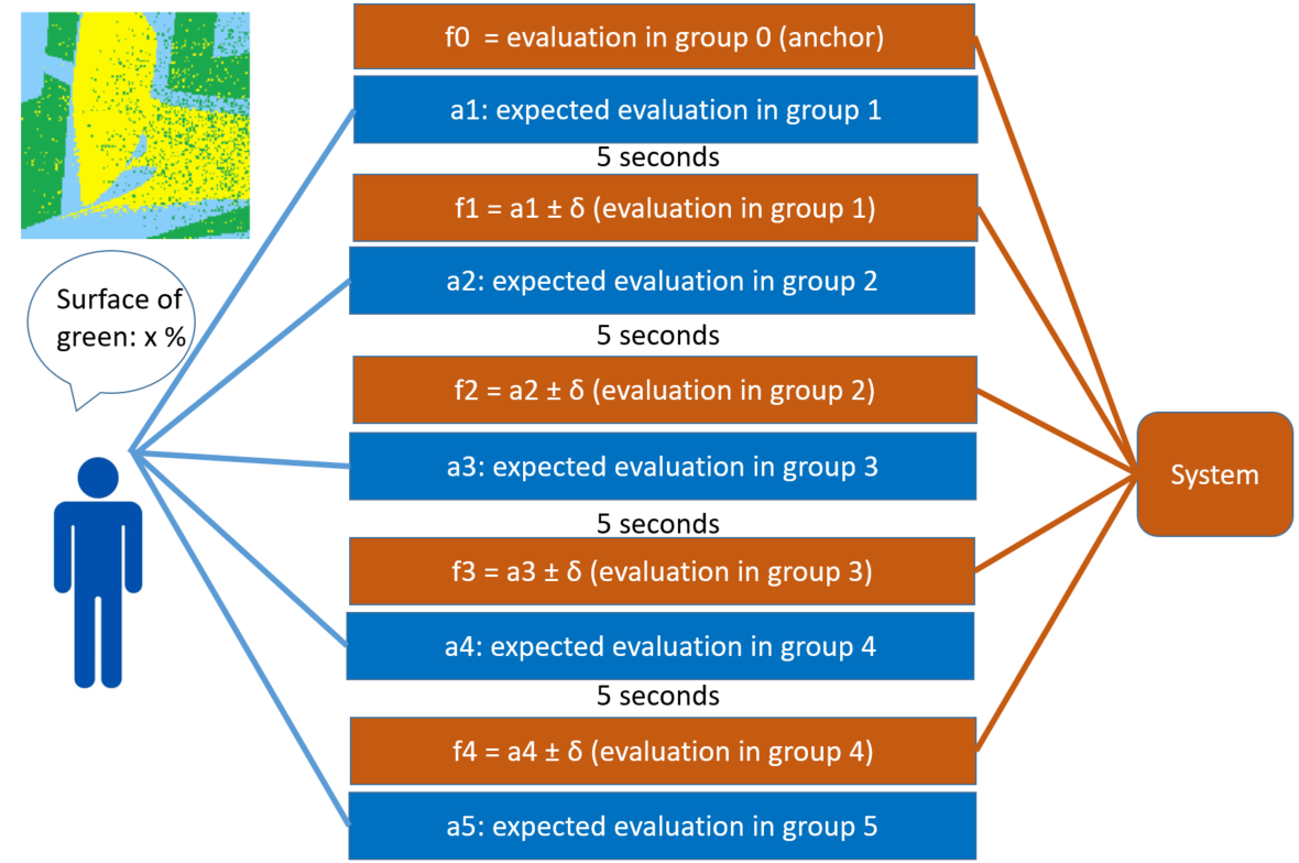
- The participants are requested to assess the size of the coloured surface in the 3 different 2D images. An example of image is shown on Figure 2.
- The participants are told that the experimenters can compute exactly their error of surface assessment on these three images and can do the same for a large number of other people who already performed the task. Moreover, the participants are told that the experimenters gathered the errors (\(G_0\) to \(G_5\)) from 6 groups of randomly chosen 100 people and that the error of the participant will be compared to the errors of these groups. An example of such an evaluation is: "you did better than 75 % of the group".
- The participants are told their evaluation \(f_0\) in group \(G_0\). Then they are asked their expected evaluation \(a_1\) in group \(G_1\). This first self-evaluation \(a_1\) is the starting point of the series of alternating feedbacks.
- The participants are asked their expected evaluation \(a_2\) in group \(G_2\). They are requested to express this self-evaluation between their previous expectation \(a_1\) and the feedback \(f_1\) that they just received. Indeed, the literature (e.g., Hovland & Sherif (1980)) and several pilot experiments that we made (not-reported here) suggest that this assumption holds in a large majority of cases. Therefore, the constraint on the self-evaluation is primarily a means to limit the noise in the results. Moreover, the way in which the sensitivity changes within the bounds, when the self-evaluation varies, is our main subject of investigation and it is not constrained.
- The same process is repeated again three times, with feedbacks \(f_2, f_3\) and \(f_4\) that are presented as the evaluation of the participant in groups \(G_2, G_3\) and \(G_4\), and requesting the participant’s expected evaluations \(a_3, a_4\) and \(a_5\) in groups \(G_3, G_4\) and \(G_5\) (interpreted as successive self-evaluations). Actually, each time, the feedbacks are computed as:
where \(a_t\) is the expected evaluation of the participant in group \(G_t\) given the last feedback \(f_{t-1}\) which is (allegedly) their evaluation in group \(G_{t-1}\). \(\delta \approx 13\) in the experiment (see details in the paper).\[\begin{aligned} f_t = a_t \pm \delta, \end{aligned}\] \[(34)\] - Finally, the participants are asked if they believed that the feedbacks were really the evaluation of their error with respect of the errors from real groups of 100 persons or if they believed that these feedbacks were manipulated by the experimenters. The participants are requested to rate their belief between 0 (the feedbacks are fake) to 10 (the feedbacks are real). In the following, we call this answer: "trust in feedback" or sometimes simply "trust" of the participant.
The sequence of positive and negative feedbacks is chosen at random in the six possible sequences that contain two positive and two negative feedbacks (see Table 1). However, in some cases, when the self-evaluation \(a_t\) is close to the limit \(1\) or \(100\), the chosen feedback would leave the [1,100] interval. In these cases, the feedback is truncated in order to remain in [1,100]. This might lead to some sequences where the positive and negative feedbacks are not balanced. We removed these sequences from the treated results.
| \(f_1\) | \(f_2\) | \(f_3\) | \(f_4\) |
|---|---|---|---|
| + | + | - | - |
| + | - | + | - |
| + | - | - | + |
| - | + | + | - |
| - | + | - | + |
| - | - | + | + |
Finally, the experiment also includes a questionnaire evaluating the self-esteem of the participants using Rosenberg’s scale (Vallières & Vallerand 1990).
Results
The experiment involves 1509 participants (803 females, 706 males, age between 17 and 79). We removed 141 participants because their series of self-evaluations got too close to 0 or 100 and we could not apply the planned feedback. In total, after these exclusions the data set includes 5472 triples \((a^i_t, f^i_t, a^i_{t+1})\) for 1368 participants (729 women and 639 men, mean age: 36.8 years). The data of the experiment and all the results are available at: https://github.com/guillaumeDeffuant/sensitivityBias. We focus here only on the most important ones and omit all the details.
The collected data allow us to compute approximations of the functions of sensitivity \(h_p\) to positive feedbacks, \(h_n\) to negative feedbacks and \(h\) to all feedbacks. These approximate function are the results of linear regressions taking the self-evaluation change \(\frac{|a_{t+1} - a_t|}{\delta}\) as output variable and the evaluation \(\frac{a_t}{100}\) as predictor variable.
More precisely, from a given data set of triples \((a^i_t, f^i_t, a^i_{t+1})\), the following linear model approximates the sensitivity to feedbacks \(h\):
| \[\begin{aligned} \frac{|a^i_{t+1} - a^i_t|}{\delta} &\approx c \frac{a^i_t}{100} + b \approx h(a^i_t). \end{aligned}\] | \[(35)\] |
We compute the regressions and the biases when mixing triples \((a^i_t, f^i_t, a^i_{t+1})\) from different participants and several time steps. The details of the results (not reported here) suggest that the self-evaluation change at the fourth time step is less reliable probably because the participants loose attention after several repetitions of the same process. Therefore, we focus on mixing times steps 1, 2 and 3. Table 2 shows the value of the slope \(c\) of the sensitivity to feedbacks and the bias from sensitivity to feedback computed with Equation 33. In order to assess the reliability of this measure, we computed its mean and the standard over 200 bootstrap samples. This table also shows the number \(N\) of triples \((a^i_t, f^i_t, a^i_{t+1})\) in each set.
| Trust | \(N\) | \(c\) | \(S\) mean | \(S\) std dev |
|---|---|---|---|---|
| \(0 \leq T \leq 10\) | \(4104\) | \(-0.09^{***}\) | \(0.59\) | \(0.17\) |
| \(T \leq 6\) | \(2484\) | \(-0.07^*\) | \(0.44\) | \(0.2\) |
| \(T \geq 7\) | \(1620\) | \(-0.13^{***}\) | \(0.94\) | \(0.28\) |
| \(T \geq 8\) | \(1251\) | \(-0.15^{***}\) | \(1.13\) | \(0.31\) |
| \(T \geq 9\) | \(843\) | \(-0.18^{***}\) | \(1.37\) | \(0.37\) |
In all cases, the value of the slope \(c\) is significantly negative, with an increasing amplitude when trust in the feedback increases. Overall these results confirm our main hypothesis that sensitivity to feedback decreases when self-evaluation increases. The confirmation is particularly clear in sets of participants reporting a high trust.
Moreover, the results of the bootstrap on the measure of the bias from sensitivity to feedback confirm that this decrease of the sensitivity induces a detectable positive bias in all the considered sets. The bias is stronger in sets of participants reporting a high trust, where it is around 1 % of the feedback intensity. This means that the average increase of the self-evaluation is about 1 % of the feedback intensity at each interaction.
This value is small, which explains why it has been overlooked up to now. This was expected, as it is of second order of the feedback intensity. However, the model suggests that these small changes could add-up over time at each interactions and finally be responsible for a much bigger distortion of self-evaluation.
Discussion
Our main objective in this paper is to show an example of opinion dynamics model suggesting an experiment that confirms the existence of yet undetected phenomenon. Moreover, this phenomenon would most probably never have been imagined without the theoretical analysis of the model. Indeed, the biases were identified in the model because their effects were easily observed in long lasting simulations, involving millions of virtual interactions. We could then detect their much smaller effect, which we had initially overlooked, on a single time step. Then understanding these observations required a significant effort of mathematical analysis.
In particular, the model reveals a positive bias in self-evaluation induced by a decreasing sensitivity to feedback. It seems almost impossible to observe this bias in real life without looking for it with specific treatments of data from a specifically designed experiment.
The paper describes such an experiment and the corresponding data treatments. The main results confirm that sensitivities to feedbacks decrease when the self-evaluation increases, because the slopes of the regressions approaching the functions of sensitivity are significantly negative. As expected, the treatments yield a significant positive bias from sensitivity. In sets of participants reporting a high value of trust, which better correspond to the theoretical assumptions, the bias is around \(1\%\) of the feedback intensity with a bootstrap standard deviation around \(0.3\).
This relatively small value explains the difficulty to detect this bias. Moreover, this effect is generally combined with the self-enhancement which tends to be higher (Deffuant et al., 2022b). Nevertheless, the long term simulations suggest that, in certain conditions, adding the small impact of the bias overtime can lead to very significant effects.
Moreover, the opinion dynamics model suggests other experiments. Firstly, we also observed a negative bias on the evaluation of others in the simulations, which is also due to the decreasing sensitivity to the feedbacks. Again, this negative bias seems absent from the literature in social sciences. We are currently designing experiments in order to detect it. Secondly, the analysis of the model dynamics shows that the positive and the negative biases combine each other with different weights depending on the position of the agents in the evaluation hierarchy: for agents located high in the hierarchy, the positive bias dominates and the average evaluation of these agents tends to increase. On the contrary, for agents situated low in the hierarchy, especially when there is gossip, the negative bias tends to dominate and the average evaluation of these agents tends to decrease. In our view, designing experiments checking these model predictions is another exciting scientific challenge.
The experimental research suggested by the model is thus at its beginning and it may be risky to draw general lessons at such an early stage. However, it seems safe to say that the specific added value from agent or opinion dynamics models, compared with more standard modelling approaches, is to reveal various mechanisms inducing the emergence of unexpected properties. Generally, understanding these mechanisms requires a significant theoretical effort. This makes them almost impossible to identify in social data that are not specifically collected with the aim to detect them. Therefore, it is necessary to design specific experiments in order to check the existence of mechanisms, or properties, identified in the model. Overall, it seems very likely that other models could also reveal yet undetected social phenomena, that are later confirmed experimentally.
An important condition is that researchers keep this approach in mind as a possibility. Indeed, it seems to us that, when relating models to data, the unquestioned mindset is to derive models from or to fit models on existing data. This approach is conform to the dominant view that models should fit reality. We do agree that this standard view is interesting and can produce good research. However, science also often progresses differently: it builds a new reality from new concepts and new experiments.
Acknowledgements
This research has been partially funded by the Agence Nationale de la Recherche in the ToRealSim project (ANR-18-ORAR-0003-01).
References
AXELROD, A. (1997). The dissemination of culture: A model with local convergence and global polarization. The Journal of Conflict Resolution, 41(2), 203–226. [doi:10.1177/0022002797041002001]
BEER, J. S. (2014). Exaggerated positivity in self-Evaluation: A social neuroscience approach to reconciling the role of self-esteem protection and cognitive bias. Social and Personality Psychology Compass, 8(10), 583–594. [doi:10.1111/spc3.12133]
BEN-NAIM, E., Frachebourg, L., & Krapivsky, P. L. (1996). Coarsening and persistence in the voter model. Physical Review E, 53(4), 3078. [doi:10.1103/physreve.53.3078]
BUEHLER, R., Griffin, D., & Ross, M. (1994). Exploring the "planning fallacy": Why people underestimate their task completion times. Journal of Personality and Social Psychology, 67(3), 366–381. [doi:10.1037/0022-3514.67.3.366]
CAMPBELL, W. K., & Sedikides, C. (1999). Self-Threat magnifies the self-Serving bias: A meta-Analytic integration. Review of General Psychology, 3, 23–43. [doi:10.1037/1089-2680.3.1.23]
CASTELLANO, C., Fortunato, S., & Loretto, C. V. (2009). Statistical physics of social dynamics. Reviews of Modern Physics, 81(2), 591. [doi:10.1103/revmodphys.81.591]
DEFFUANT, G., Bertazzi, I., & Huet, S. (2018). The dark side of gossips: Hints from a simple opinions dynamics model. Advances in Complex Systems, 21, 1–20. [doi:10.1142/s0219525918500212]
DEFFUANT, G., Carletti, T., & Huet, S. (2013). The Leviathan model: Absolute dominance, generalised distrust and other patterns emerging from combining vanity with opinion propagation. Journal of Artificial Societies and Social Simulation, 16(1), 5. [doi:10.18564/jasss.2070]
DEFFUANT, G., Huet, S., & Skerratt, S. (2008). An agent based model of agri-Environmental measure diffusion: What for? In A. Lopez Paredes & C. Hernandez Iglesias (Eds.), Agent based modelling in natural resource management (pp. 55–73). Valladolid: INSISOC.
DEFFUANT, G., Neau, D., Amblard, F., & Weisbuch, G. (2000). Mixing beliefs among interacting agents. Advances in Complex Systems, 3, 87–98. [doi:10.1142/s0219525900000078]
DEFFUANT, G., Roozmand, O., Huet, S., Kahmzina, K., Nugier, A., & Guimond, S. (2022a). Can biases in perceived attitudes explain anti-Conformism? IEEE Transactions on Computational Social Systems, 10(3), 922–933. [doi:10.1109/tcss.2022.3154034]
DEFFUANT, G., & Roubin, T. (2022). Do interactions among unequal agents undermine those of low status? Physica A: Statistical Mechanics and Its Applications, 592, 126780. [doi:10.1016/j.physa.2021.126780]
DEFFUANT, G., Roubin, T., Nugier, A., & Guimond, S. (2022b). A newly detected bias in self-evaluation. HAL - Open science. Available at: https://hal.science/hal-03790992/document
DITTO, P. H., & Boardman, A. F. (1995). Perceived accuracy of favorable and unfavorable psychological feedback. Basic and Applied Social Psychology, 13, 137–157. [doi:10.1207/s15324834basp1601&2_9]
DUNNING, D., Heath, C., & Jerry, S. (2004). Flawed self-Assessment. Implications for health, education and the workplace. Psychological Science in the Public Interest, 21, 69–106. [doi:10.1111/j.1529-1006.2004.00018.x]
DUNNING, D., & Story, A. L. (1991). Depression, realism, and the over-confidence effect: Are the sadder wiser when predicting future actions and events? Journal of Personality and Social Psychology, 61(4), 521–532. [doi:10.1037/0022-3514.61.4.521]
EPLEY, N., & Dunning, D. (2000). Feeling holier than thou: Are self-serving assessments produced by errors in self or social prediction? Journal of Personality and Social Psychology, 79(6), 861–875. [doi:10.1037/0022-3514.79.6.861]
FISCHHOFF, B., Slovic, P., & Lichtenstein, S. (1977). Knowing with certainty: The appropriateness of extreme confidence. Journal of Experimental Psychology: Human Perception and Performance, 3(4), 552–564. [doi:10.1037/0096-1523.3.4.552]
FLACHE, A., Mäs, M., Feliciani, T., Chattoe-Brown, E., Deffuant, G., Huet, S., & Lorenz, J. (2017). Models of social influence: Towards the next frontiers. Journal of Artificial Societies and Social Simulation, 20(4), 2. [doi:10.18564/jasss.3521]
GALAM, S. (2002). Minority opinion spreading in random geometry. The European Physical Journal B, 25(4), 403–406. [doi:10.1140/epjb/e20020045]
GRIFFIN, D., Dunning, D., & Ross, I. (1990). The role of construal processes in overconfident predictions about the self and others. Journal of Personality and Social Psychology, 59(6), 1128–1139. [doi:10.1037/0022-3514.59.6.1128]
HEGSELMANN, R., & Krause, U. (2002). Opinion dynamics and bounded confidence: Models, analysis and simulation. Journal of Artificial Societies and Social Simulation, 5(3), 2.
HOVLAND, C., & Sherif, M. (1980). Social judgment: Assimilation and contrast effects in communication and attitude change. Greenwood.
HUET, S., & Deffuant, G. (2010). Openness leads to opinion stability and narrowness to volatility. Advances in Complex Systems, 13(3), 405–423. [doi:10.1142/s0219525910002633]
JAGER, W., & Amblard, F. (2005). Uniformity, bipolarization and pluriformity captured as generic stylized behavior with an agent-Based simulation model of attitude change. Computational & Mathematical Organization Theory Volume, 10, 295–303. [doi:10.1007/s10588-005-6282-2]
KLEMM, K., Eguíluz, V., Toral, R., & San-Miguel, M. (2003). Global culture: A noise-induced transition in finite systems. Physical Review E, 67(4), 045101. [doi:10.1103/physreve.67.045101]
KRAPIVSKY, P. L., & Redner, S. (2003). Dynamics of majority rule in two-State interacting spin systems. Physical Review Letters, 90(23), 238701. [doi:10.1103/physrevlett.90.238701]
LEARY, M. R., Tambor, E., Terdal, S., & Downs, S. (2005). Self-Esteem as an interpersonal monitor: The sociometer hypothesis. Journal of Personality and Social Psychology, 16(11), 76–111. [doi:10.1037/0022-3514.68.3.518]
MARTINS, A. C. R. (2008). Continuous opinions and discrete actions in opinion dynamics problems. International Journal of Modern Physics C, 19(4), 617–624. [doi:10.1142/s0129183108012339]
MÄS, M., & Flache, A. (2013). Differentiation without distancing. Explaining bi-Polarization of opinions without negative influence. PLoS One, 8(11), e74516.
MÄS, M., Flache, A., & Helbing, D. (2010). Individualization as driving force of clustering phenomena in humans. PLoS Computational Biology, 6(10), e1000959.
MISCHEL, W., Ebbesen, E. B., & Zeiss, A. R. (1976). Determinants of selective memory about the self. Journal of Consulting and Clinical Psychology, 29, 279–282. [doi:10.1037/0022-006x.44.1.92]
MORELAND, R. L., & Sweeney, P. D. (1984). Self-expectancies and relations to evaluations of personal performance. Personality, 52(2), 156–176. [doi:10.1111/j.1467-6494.1984.tb00350.x]
SEDIKIDES, C., & Gregg, A. P. (2003). Portraits of the self. In A. Hogg & J. Cooper (Eds.), The SAGE handbook of social psychology (pp. 93–122). Thousand Oaks, CA: Sage. [doi:10.4135/9781848608221.n5]
SKOWRONSKI, J. J., Betz, A. I., Thompson, C. P., & Shannon, L. (1991). Social memory in everyday life: Recall of self-Events and other-Events. Jounral of Personality and Social Psychology, 68, 247–260. [doi:10.1037/0022-3514.60.6.831]
SOOD, V., & Redner, S. (2005). Voter model on heterogeneous graphs. Physical Review Letters, 94(17), 178701. [doi:10.1103/physrevlett.94.178701]
SZNAJD-WERON, K. (2002). Controlling simple dynamics by a disagreement function. Plysical Review E, 66(4). [doi:10.1103/physreve.66.046131]
VALLIÈRES, E., & Vallerand, R. (1990). Traductuion et validation canadienne-française de l’échelle de l’estime de soi de rosenberg. International Journal of Psychology, 25(2), 305–316. [doi:10.1080/00207599008247865]
VALLONE, R. P., Griffin, D., Lin, S., & Ross, L. (1990). Overconfident prediction of future actions and outcomes by self and others. Journal of Personality and Social Psychology, 58(4), 582–592. [doi:10.1037/0022-3514.58.4.582]
ZUCKERMAN, M. (1979). Attribution of success and failure revisited, or: The motivational bias is alive and well in attribution theory. Journal of Personality, 47(2), 245–287. [doi:10.1111/j.1467-6494.1979.tb00202.x]