Network Structure Can Amplify Innovation Adoption and Polarization in Group-Structured Populations with Outgroup Aversion

, ,
and
aUniversity of Central Florida, United States; bUniversity of Central Florida, UCF Coastal: National Center for Integrated Coastal Research, United States
Journal of Artificial
Societies and Social Simulation 26 (4) 4
<https://www.jasss.org/26/4/4.html>
DOI: 10.18564/jasss.5167
Received: 29-Jun-2022 Accepted: 10-Jun-2023 Published: 31-Oct-2023
Abstract
Individuals’ decisions to adopt an innovation can be influenced by the frequency of other adopters as well as by the group membership of previous adopters or non-adopters in their social network. In addition, adoption or non-adoption of some innovations has been characterized as a means of signaling identification with a group. While identity signaling and outgroup aversion effects on adoption and polarization have been considered in a geo-spatial environment, this work extends an existing model of outgroup aversion to a network-based environment. The results show that adoption levels in a network environment were higher, and polarization lower compared to the non-network environment with all other factors fixed. As more factors were varied, the associated change to adoption and polarization were amplified in network environments. The two most significant factors influencing adoption variability were the degree of outgroup aversion and the level of frequency dependence. Finally, in network environments with outgroup aversion, adoption was found to be higher when modularity and eigenvector centrality were high. In today’s polarized social environment, understanding these effects is critical to the adoption of emerging innovations such as mitigating climate change, combating novel viruses, or decentralizing financial transactions. While innovators are often focused on solving technical challenges to advance adoption of an innovation, equal emphasis on understanding and solving social and potential outgroup effects will be needed to achieve a desired adoption level.Introduction
Social aspects of innovation
An innovation is an idea, practice, or object that is perceived as new by an individual or entity and adds value (Miller et al. 2021; Rogers 2003). Innovation diffusion is described as “a process through which (1) an innovation (2) is communicated through certain channels (3) over time (4) among the members of a social system” (Rogers 2003). Rogers also classifies categories of adopters into innovators, early adopters, early majority, late majority and laggards (Rogers 2003). In a marketing context, to predict new product sales, Bass developed analytic equations related to the innovation concepts from Rogers that separated adopters into “innovators” and “imitators” (Bass 1969). Imitators encompass the categories following innovators, reflecting the s-curve of adoption (Bass 1969). Imitation processes also have a deep trajectory in evolutionary social learning (Boyd & Richerson 1988; Henrich & Boyd 1998). Rand & Rust (2011) adapted the Bass model to an agent-based model in a network environment, showing that the results from Bass can be replicated with heterogenous agents, in a stochastic adoption process on a network. The network adaptation helped to account for imperfect mixing characteristics of adopter populations. Smaldino et al. (2017) took this idea further by introducing an agent-based model with outgroup effects that may resist or accelerate adoption decisions when the innovation has overt identity signaling of group membership. While the Smaldino et al. (2017) model proposes a method to model the outgroup factor, it does not consider the adoption process with outgroup effects in a network-based environment.
Resistance to technical solutions may occur due to the presence of polarized groups who believe or do not believe in the benefit of an innovation. The term, outgroup aversion, refers to the impact that group affiliation may have on innovation adoption (Berger & Heath 2008). Despite the intrinsic benefit that a technology may have, the adoption decision may be based more on the affiliation of adopters to a group for which the potential adopter is not a member. The probability of adopting a new product or agreeing to collective action is reduced when adoption causes undesirable identity signaling with respect to being affiliated with the outgroup (Berger & Heath 2007). In Smaldino et al. (2017), this effect on adoption was referred to as the ingroup-outgroup bias factor. This factor is coupled with a frequency dependence factor to formulate an adoption probability. The frequency dependence factor was an adapted form of the imitation factor for product adoption (Bass 1969).
Agent-based modeling has been used to simulate adoption due to its ability to model heterogenous agents, self-organizing behavior, and emergent outcomes (Rand & Rust 2011). Agent-based approaches were used to simulate imperfect mixing and to capture the stochastic properties of agents as well as the geo-spatial characteristics. Smaldino et al. (2017) used agent-based models to demonstrate adoption-driven identity signaling with skewed group membership in a geo-spatial line grid. This research extends the Smaldino et al. (2017) model to understand outgroup effects on adoption in a network environment. The model focused on adoption differences between groups within grid squares with different proportions of group membership, with local adoption being within a grid square and global adoptions being the total over all squares. The Smaldino et al. (2017) model was used as a baseline, keeping the equations and variables consistent to understand the net effect of introducing a social network structure. The research question explored for this study is, “what is the impact of outgroup aversion on innovation adoption and polarization on a network?” The hypotheses were generated by considering the structural differences between network environments and the line grid baseline model. Three hypotheses were tested:
- Hypothesis One: Stabilized adoption and polarization with an outgroup factor present and default parameter values will be different for a skewed lattice network than for a line grid baseline.
- Hypothesis Two: Stabilized adoption and polarization with an outgroup factor
- differ from a line-grid baseline by network type (lattice, random, small world, and scale-free) and
- are directionally impacted by network characteristics (average eigenvector centrality, average betweenness centrality, mean path length, modularity, and average clustering coefficient).
- Hypothesis Three: Modifying all the parameters, in addition to the environment type, results in significant impacts to adoption and polarization.
In this research, agents are interacting with other agents in various types of network structures. Network environments are a foundational component of social systems as a key mechanism for the transmission of information, ideas and relationships between people (Borgatti et al. 2009; Freeman 2000). The focus of this study is on adoption and polarization effects related to network structure in the presence of outgroup factors. Outgroup factors are present when adoption behavior is impacted by agents observing both group membership and adoption behavior in making an adoption decision. The term “outgroup” refers to an observed individual’s group membership being different than the group of the agent who is observing.
Outgroup effects are particularly relevant in today’s polarized environment (Garibay et al. 2019; Klein 2020). Innovation in a polarized environment is applicable in many areas of emerging innovations. Examples include climate change innovations, vaccine adoption for combating novel viruses and efforts to decentralize financial transactions with blockchains and crypto technology. In climate change, groups may form into climate change deniers versus climate change doomsayers along political lines. For vaccines, political group membership may be one of several factors influencing vaccination rates. Decentralized finance or cryptocurrency adoption may have potential groups related to technologists vs. non-technologists where buying and selling products in a primitive market may divide participants into groups supporting or opposing digital currencies.
Previous research
The foundational literature as the basis for this research covers the topics of innovation adoption, imitation effects, network science, social networks, imitation, groups and outgroups, identity signaling and diffusion. Since the topic spans disciplines and research traditions in sociology, network science, marketing, psychology, biology, and physics, the collective group of foundational research will be compared across themes to show the gap that this research seeks to explore.
Rogers (2003) provides a detailed history of innovation diffusion starting with the concept of imitation from Tarde (1903) and the initial notions of outcasts from a system and the early beginnings of social network formation from Simmel (1964), Simmel (1922). Rogers’ contribution to the spread of innovations was the notion of the s-shape curve that defines the cumulative adoption cycle starting with adopter categories as innovators, early adopters, early majority, late majority and laggards (Rogers 2003). Bass uses this to analytically describe the equations to generate such a curve over time (Bass 1969). The analytic model first introduced the concept of an innovator effect (p) and an imitation effect (q) and were validated against new product introductions in the late 1960’s such as washing machines and televisions (Bass 1969).
Two comprehensive studies of innovation diffusion literature provide context for this study and gaps. In Keisling et al. (2012), a framework was introduced to classify agent-based models of consumer adoption behavior and social influences as well as theoretical findings from the influence of consumer heterogeneity, social influence and promotional strategy effectiveness. Zhang & Vorobeychik (2019) updated Kiesling and provides a systemic review of literature regarding empirically grounded agent-based models of innovation diffusion and a discussion of the issues of validation and calibration. Based on the classification of these two survey studies, this research extends an existing threshold-based social influence model by adding network-based interaction environments to the existing model’s environment of cliques of agents on a line-grid. In these reviews, there are references to social influence and opinion dynamics models which drive opinion convergence, group formation and ultimately adoption decisions; however, none of the previous literature makes a direct reference to explicit outgroup effects on adoption in network environments.
The group aspect of this topic merits inclusion of additional literature to consider aspects of imitation, outgroup behavior and identity signaling. Some aspects of group formation can be considered in opinion dynamics models of innovation diffusion; these models may be instrumental in the formation process of groups based on opinion convergence or divergence. Deffuant et al. (2005) provides a model in this regard to show the dynamics of personal payoffs and social influence before an adoption decision is made. Mutlu & Garibay (2021) considers degree dependent threshold models of opinion dynamics for online social networks.
Imitation effects were not limited to the study of innovation. Boyd & Richerson (1988) put together a theory of using imitation as a basis of social learning, culture transmission and the evolution of different cultures despite genetic similarity of humans. These ideas are further explored by Henrich & Boyd (1998) to show the cultural effects of imitation or conformism among groups . The concepts from these two sources justify the use of a frequency dependence or imitation term in the adoption probability calculation in the proposed model. In none of these models are the dynamics of outgroups or identity signaling through adoption or non-adoption addressed in the adoption decision.
The network environment proposed by the models have a history across multiple disciplines. Random networks were described and explored by Erdos & Renyi (1960). A general history of networks across disciplines is described by Barabasi (2016). Borgatti describes the role of networks from a range of disciplines from psychology, political science, anthropology and economics (Borgatti et al. 2009). One of the first examples of the role networks play in imitative behavior was in Moreno’s study of runaways at an orphanage that was tied to social network connections (Borgatti et al. 2009; Moreno 1934). A significant development was the discovery of the concept of “small world” networks (Watts & Strogatz 1998) that helped to explain the “six degrees” problem in Milgram (1967) and the strength of weak ties (Granovetter 1973). Mapping degree distributions of real networks from power grids, highway systems, airline routes, the world-wide web and the internet showed that many networks had a structure defined by a preferential attachment mechanism i.e. new nodes are not attached randomly but prefer nodes with higher number of connections or edges (Barabasi & Albert 1999). The degree distributions for these follow a power law curve (Barabasi & Albert 1999). These random, small world and preferential attachment networks inform the network environment decisions for the model used. Network science continues to be explored to understand phenomenon in many disciplines ranging from sociology to socio-ecological systems to biology to online social network analysis. Of particular importance to the understanding of group phenomenon is the ability to identify communities defined by non-random connections between nodes. This concept was first developed in the study of groups and subgroups in the social sciences (Wasserman & Faust 1994). Methods to efficiently determine these network driven communities were developed by Newman (2006) and referred to as modularity. The other choices of network metrics were informed by the metric descriptions in Barabasi (2016) and Newman (2018).
Innovation adoptions diffusing across a network environment have been characterized as a complex contagion process (Centola & Macy 2007). A complex contagion requires more than one exposure unlike phenomena such as the spread of a virus or the six degrees problem (Centola & Macy 2007). The complex contagion mechanisms between nodes inform the adoption probability calculation in the model. Also related to the dynamics of calculating the adoption probability, are the effects of identity signaling to inform ingroup affinity and outgroup aversion (Berger & Heath 2007, 2008). Berger and Heath do not consider the effects explicitly on adoption or in a network environment. Schelling’s early work on segregation models was a variant of the decision process (moving out of a neighborhood) related to the effect of a group-derived fitness defined as a tolerance percent (Schelling 1971). Smaldino takes this idea further by developing an outgroup factor composed of assessing neighborhood and local nodes to modify the imitation factor to result in either a higher or lower probability of adopting (Smaldino et al. 2017).
The use of agent-based models for simulating complex phenomenon have evolved over time and are considered in this review. Agent-based models were first pioneered by Schelling (1971) using physical agents and manual decision rules to simulate segregation in neighborhoods. Agent-based models have gained acceptance for modeling complex adaptive systems due to their ability to simulate non-linear systems, handle probabilistic stochastic processes, determine previously undetected emergent outcomes, and to handle a heterogenous subject populations (Rand & Rust 2011). Goldenberg has extensively modeled innovation adoption on networks (Goldenberg et al. 2001, 2007, 2009). One key contribution of Goldenberg was the development of models of social networks on which agent-based model simulations were used to understand the role of hubs in product adoption (Goldenberg et al. 2009). Rand & Rust (2011) describes a simplified model that accurately simulated product adoption data sets from Bass (1969). However, this model did not allow for anything less than a full adoption after enough time transpires and did not consider the impact of opposing groups’ on adoption. Additionally, Garibay et al. (2021) provides a framework for modeling information spread on social networks using agent-based models.
While much of the existing research covers one or more of the interdisciplinary topics, a gap exists to understand the research question of understanding innovation adoption with outgroup aversion effects on a network. Table 1 summarizes the themes of the research considered.
Network adaptations
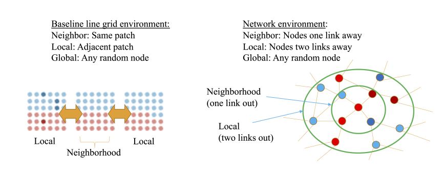
Extending the model to a network environment improves two areas of the baseline model: the environment characteristics and the observer mechanism. Within each grid square on the original line grid model, the agents can be assumed to be in a clique. From a network perspective, a clique structure means that each node is connected to all other nodes, given there is an equal probability of being included in the observations for making an adoption decision. The baseline model had 30 fixed observations that are based on sampling from the neighborhood (a grid square containing 6 x 6 agents), then sampling locally from an adjacent grid or globally from anywhere. In either case, an agent may not get sampled or could be sampled multiple times. In complex contagion networks, multiple sources are more critical than the number of exposures to the sources (Centola & Macy 2007). In a network, neighborhoods are defined as all first-degree nodes (Barabasi & Albert 1999). The high number of neighbors in a clique implies a high number of “influencers” for an adoption decision. Dunbar (1992) has shown that for a purchase decision, five to six influencers exist, related to the number of “close relationships”, which is also consistent with complex contagion dynamics requiring multiple influencers (Centola & Macy 2007).
For these reasons, the observer mechanism consisted of a network with approximately six neighbors. For the observations, all immediate neighbors’ information was considered by using the neighborhood definition from network science as the first degree nodes connected to a given node (Barabasi 2016). The "local" view was assumed to be two links out to reflect geo-spatial location in close physical proximity to the neighborhood. The choice of two links as the local view was derived to be consistent with the baseline model where "local" was defined as the adjacent cliques in the line grid, or effectively one step out of the clique in either direction (Figure 1). Additionally, any more than two links out would encompass a substantial portion of the network especially for the scale-free network where the mean shortest path length is small. The "global" view is consistent with baseline model, as any random node in the environment. Finally, "neighborhood" observations as a proportion of total observations is defined as a variable, f. The total observations before an adoption decision may vary based on the proportion f, and therefore is a much smaller number than the 30 fixed observations in the baseline model. The concepts of neighborhood, local view and global view are shown in Figure 1.
Network metrics
The type of network i.e. lattice, small-world, scale-free and random networks can be analyzed to determine impacts on adoption and polarization at both global and local levels. In addition , independent of network type, quantitative network characteristics were also considered. The metrics chosen for examination are meant to be an initial examination of top-line characteristics related to node centrality, betweenness, distance between nodes, modularity and clustering characteristics. The metrics used are by no means exhaustive, but an initial starting point for further investigation. For this research five core network metrics were evaluated to understand their impact on adoption and polarization:
- Betweenness centrality: For a given node, betweenness centrality is the number of shortest paths that must pass through it to get to another node in the network. It can show the criticality of a node in acting as a gatekeeper for communicating information between nodes and may impact the rate at which adoption spreads across a network.
- Eigenvector Centrality: Eigenvector centrality provides a balanced measure of the importance of a node with respect to its connections to other nodes, taking into consideration the importance of the connected nodes (Newman 2018). In an adoption mechanism a high eigenvector centrality may be a sign of a high influencer to encourage or discourage adoption.
- Mean shortest path length: A measure of the average number of “jumps” needed by each node to reach all other nodes in the network gives a sense of the small world effect of “six degrees” referenced by Watts & Strogatz (1998), Granovetter (1973) and Milgram (1967). In an adoption diffusion process, a lower mean shortest path length would enable a more efficient transmission of information to all potential adopters. This metric is undefined when there is more than one giant component. Only networks with one giant component were considered to ensure this effect can be measured and to ensure multiple components from network generation was not a spurious cause for non-adoption (i.e., a source of statistical noise).
- Average local clustering coefficient: this measure was used to understand the degree to which an individual connected to two other individuals who are also connected with each other. Clustering reduces the number of “structural holes” between nodes to provide more than one source of information for making decisions (Borgatti et al. 2009).
- Modularity: Modularity is most often used to assess the alignment between group membership and network structure compared to a random reference point. For most of the networks considered, this was effectively zero because group membership was distributed randomly and not used in the algorithms to generate the network. However, for the lattice network the network formation process did produce a level of modularity that could be tested for its effect on adoption (Newman 2006).
Methods
The approach was to first make a comparison between the line grid baseline by changing the structure from a clique to a network structure by connecting the nodes into a lattice network and changing the observation mechanism to ensure that all neighborhood nodes would be included in the observation. The second element of comparison was to use the lattice network as the starting point to compare other network structures.
Networks used
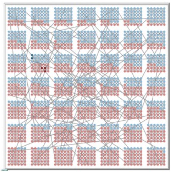
The first step in the model is to create the environment on which the adoption process will take place. Multiple network environments were tested with the modified model. A simple lattice network was created using the baseline environment and extending links within a radius of one from each agent. Additionally, to ensure a connected component, a random proportion of agents are reconnected to other agents. With this wiring, the network resembles a hybrid between a lattice and a small-world network. A modified lattice with random connections is shown in Figure 2. The red and blue nodes represent group membership and the proportions of red or blue skew within each grid square can be seen in Figure 2. The wiring across grid squares are the random reconnections to ensure the network is a connected component. The dark red or dark blue nodes indicate the early adopters’ initial position. Other networks were also tested with a consistent number of nodes and edges, all with an average degree of approximately six. The other networks consisted of a random network (Erdos & Renyi 1960), a pure small world network (Watts & Strogatz 1998), and a scale-free network (Barabasi & Albert 1999). These networks were selected as frequently referenced structures from literature covering a range of degree distributions and characteristics (Newman 2018).
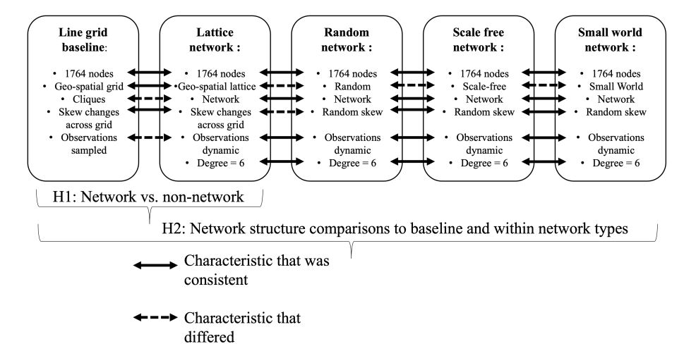
For this study, the non-lattice network models were adjusted to give approximately equal numbers of nodes and edges of each network option, using the degree consistent with the lattice option. See the Appendix for the node and edge counts by network type. Figure 3 shows how the two hypotheses span the environments considered and what variables were modified for these tests.
The model and variables
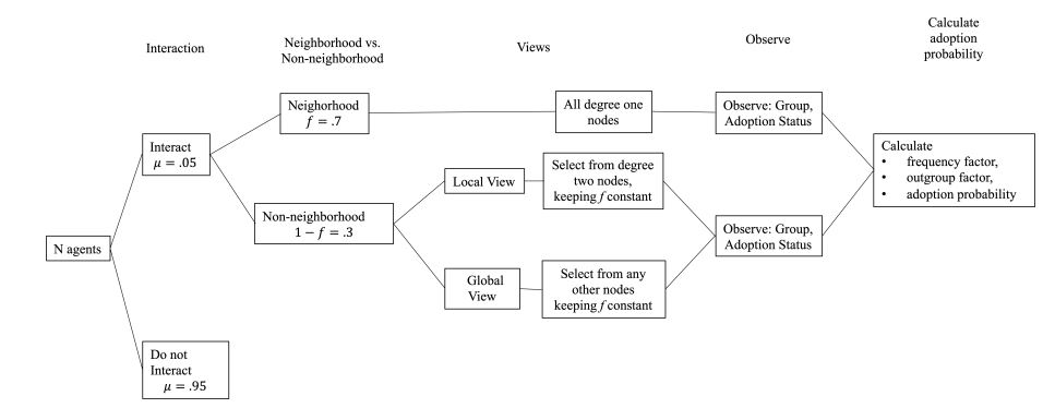
Figure 4 provides a visualization of the decision tree for an agent at each time increment in the model. The probability \(\mu\) defines the likelihood of an interaction. The interaction probability represents the portion of the population that will be making an adoption decision at any particular time interval. The model consists of agents who observe other agents in their immediate neighborhood, followed by observing agents beyond their neighborhood: either one step removed from the neighborhood observation range (local observer view) or randomly in the environment (global observer view). These act as proxies for the influence of close relationships vs. indirect influence factors. The proportion of neighborhood observations to total observations is the ratio, f. This ratio allows varying the level of influence between close relationships (neighborhood) vs. more indirect influences (local or global observer views).
The agent-based model uses an adoption probability from the baseline model based on a frequency dependence or imitation factor (F) and an outgroup aversion factor (V) as in Equations 1 and 2.
| \[ P(adoption) = (Frequency\hspace{4pt} dependence)\times (Outgroup \hspace{4pt}aversion)= \textit{F}\times \text{V}\] | \[(1)\] |
| \[ P(adoption) = F\times V = x^\lambda \times (1-b+\frac{b}{(1+exp(-(m_I-m_O)))})\] | \[(2)\] |
Where: x = proportion of agents who adopted, textit\(\lambda\) = strength of frequency dependence, b = strength of outgroup aversion, \(m_I\) = number of observed agents in the ingroup who have adopted, \(m_O\) = number of observed agents in the outgroup who have adopted.
The total observations (n) are tallied into totals of how many adopted in the agent’s ingroup (\(m_I\)) and how many adopted in the outgroup (\(m_O\)). The frequency dependence factor is based off the proportion of observed agents who have adopted (x), or (\(m_I\) + \(m_O\)) /n with an exponential parameter, \(\lambda\), to express the strength of frequency dependence or imitation. The difference between ingroup and outgroup adopters (\(m_I\) - \(m_O\)) is then used with the outgroup aversion parameter (b) to calculate outgroup aversion component of the adoption probability. When b equals zero, the outgroup factor is one, leaving the adoption probability based solely on frequency dependence.
In the line-grid baseline, another parameter, skew (Q), is the maximum proportion of agents that are in one group or another. For example, if Q equals .5, then all grids have an equal portion (50%) of group one and group two agents; if Q equals .9, then there is a gradation from 10% of one group at one end of the grid to 90% of the same group at the other end of the grid, with incremental increases in between. Skew was used to understand if the base membership in groups at the neighborhood level may be a factor in adoption or not. Table 2 summarizes the variable descriptions, the range of each and the default values.
| Variable | Description | Range | Default value |
|---|---|---|---|
| Environment type | Geospatial agent set-up | Line grid & 4 networks | Line grid baseline |
| \(\mu\) - interaction probability | Likelihood of interacting | .01 to 1 | .05 |
| f - immediate neighbor view probability | Proportion of observations that are immediate neighbors | 0 to 1 | .7 |
| Seeds for early adopters | Number of initial adopters | Fixed | 5 |
| Q - skew of groups group within grid squares | Maximum proportion of one in a grid square | .5 to .9 | .9 |
| b - outgroup aversion factor | Parameter of outgroup factor strength | 0 to 1 | 1 |
| \(\lambda\) - frequency dependency factor | Parameter of frequency dependence strength | 0 to 1 | .3 |
| Observer view: non-neighborhood | Observer view beyond neighborhood | local or global | local |
| Observations - line grid baseline only | The number of observations made before calculating adoption probability | Fixed | 30 |
| \(m_I\) | Number of observed ingroup agents that have adopted | Calculated | |
| \(m_O\) | Number of observed outgroup agents that have adopted | Calculated | |
| x | Proportion of observed agents that have adopted | Calculated | |
| \(n_1\) | Number of agents that have adopted from group 1 | Calculated | |
| \(n_2\) | Number of agents that have adopted from group 2 | Calculated | |
| \(n\) | Total number of adopters | Calculated | |
| \(N\) | Total number of agents | Fixed | 1,764 |
The mechanism of calculating observations from which \(m_I\) and \(m_O\) are derived in equation (2) was modified to consider network characteristics and the lower number of influencers that impact the adoption decision. The following assumptions were made with respect to the dynamics of adoption from a network diffusion perspective:
- The parameter f, which is the proportion of observations from a neighborhood will be preserved.
- For the neighborhood, all neighbors will be observed for whether each adopted and their group affiliation. The neighborhood observation will be a census of all neighbors versus a sampling.
- The local observation view pertains to those nodes that are two links out. These are selected to ensure the value of f is maintained.
To accomplish the first assumption, the number of observations were calculated dynamically while preserving the neighborhood proportion, f. For example, for the average case with a node of degree of six, a neighborhood proportion of .7, and a local observer view the neighborhood would consist of observing all six immediate neighbors, and then sampling from the 30 nodes (6 nodes x 5 links each) that are two links out to maintain the neighborhood proportion, f. An example calculation is provided in the Appendix, Local observer view example.
Outcome measures: Adoption and polarization
At each time increment, based on the observations and parameter values, the adoption probability is calculated and an adoption decision is made for the agents. Following the adoption decision, adoption and polarization are calculated in equations (3) and (4). Adoption and polarization are calculated in Equations 3 and 4.
| \[ Adoption = \dfrac{(n_1+n_2)}{N}\] | \[(3)\] |
| \[ Polarization = \dfrac{|n_1-n_2|}{(n_1+n_2)}\] | \[(4)\] |
Experiment design
To make a clear comparison to the lattice baseline, the default values from Smaldino et al. (2017) were kept consistent. The only variable modified in the first two experiments was the environment type (five values: a line grid baseline and four network structures). Fifty replications were done for each unique combination due to the stochasticity of the initial conditions. The experiment designs for the hypotheses are shown in Tables 3 and 4. The data from the second experiment was also used to explore the network characteristics; however, the analysis was directional given the network characteristics were not able to be orthogonally tested. In Table 4, the skew, Q, was set to .5 given the additional networks did not utilize the grid structure. The experiment was run using Netlogo and BehaviorSearch to do the experiment (Wilensky 1999).
| Environment | Observer | Q | f | \(\lambda\) | b | seeds | Observations | Replications |
| Type | View | |||||||
| Line grid baseline | Local | .9 | .7 | .3 | 1 | 5 | 30 | 50 |
| Lattice Network | Local | .9 | .7 | .3 | 1 | 5 | Dynamic | 50 |
| Environment | Observer | Q | f | \(\lambda\) | b | seeds | Observations | Replications. |
| Type | View | |||||||
| Line grid baseline | Local | .9 | .7 | .3 | 1 | 5 | 30 | 50 |
| Lattice Network | Local | .9 | .7 | .3 | 1 | 5 | Dynamic | 50 |
| Random Network | Local | .9 | .7 | .3 | 1 | 5 | Dynamic | 50 |
| Scale-free Network | Local | .9 | .7 | .3 | 1 | 5 | Dynamic | 50 |
| Small-world Network | Local | .9 | .7 | .3 | 1 | 5 | Dynamic | 50 |
These first two experiments isolate the influence of the environment on adoption and polarization. The last experiment, shown in Table 5, was done to explore the sensitivity of other variables in the model in addition to the environment. The total unique factorial combinations were 540 with 50 replications and 27,000 total runs.
| Factor | Levels | Values | Relevance |
|---|---|---|---|
| Environment type | 5 | Line grid baseline, lattice | May differ based on the |
| type | network, random network | relationship of stakeholders to | |
| scale free network, | the adoption decision | ||
| small world network | |||
| Observer view | 2 | Local, global | This may impact the role of global messaging |
| versus behavior of relationships | |||
| Local Maximum | 2 | 0.5, 0.9 | Tests the role of neighborhood |
| Skew, Q | adoption or resistance | ||
| Neighborhood | 3 | 0.3, 0.5, 0.7 | Tests the role of neighborhood |
| view proportion, f | influences or relationships | ||
| Frequency | 3 | 0.3, 0.5 0.7 | Tests the peer pressure of others’ |
| dependence, \(\lambda\) | adoption or non-adoption | ||
| to a solution | |||
| Outgroup | 3 | 0.0, 0.5, 1 | Tests the impact of identity with |
| factor, b | groups to adopt or not adopt |
Data
For each replication a network was generated and its quantitative characteristics recorded. The network metrics were taken for each network generated and analyzed to understand if the network structural characteristics impacted adoption and polarization. Because these metrics were an outcome of the stochastic process of generating the network, their values will be directional and not orthogonal for modeling the outcomes based on these metrics. After 1000 time-steps, the polarization and adoption were recorded as the average of the last 100 time-steps. This ensured that the recorded adoption was not a single point but a steady state average and not due to random variation. Additionally, for each replication, the five key network metrics were calculated and collected: average betweenness centrality, average local clustering coefficient, eigenvector centrality, mean shortest path length, and modularity.
The results of the experiment were exported to a file for analysis in Python using Pandas. Representative networks were exported to Python Networkx as adjacency matrices to observe characteristics of an example of each network type (Hagberg et al. 2008). The statistical analysis was done in Minitab version 21 (Minitab 2021). Analysis of Variance (ANOVA) was used to analyze experiments with more than one variable to understand which factors had the greatest explanatory power and to quantify the unexplained variance due to the inherent noise of the model due to its stochastic nature. The general linear model with stepwise forward information criteria was used with Bayesian Information Criteria (BIC) to find the most parsimonious model by minimizing BIC. Starting with a one variable model, Minitab automates finding the best model with one, two, three etc. variables, and then selects the model by minimizing BIC (Burnham & Anderson 2004). The details of the results of this process are in the Appendix. To test for multi-collinearity, variance inflation factors (VIF) were examined, which was critical for examining interaction effects. The model building consisted of an iterative process of identifying the most parsimonious models, checking for multicollinearity and ensuring that all factors were statistically significant.
Results
The main results were that a network environment does make a difference in the pattern of adoption diffusion. Keeping all else equal with default values, the line-grid baseline and connected lattice network showed a significant difference in adoption and polarization with higher adoption rates and lower polarization on the network. Comparing line-grid baseline to various other network types also showed differences. Eigenvector centrality and modularity values were positively correlated with adoption levels. When all relevant variables are systematically varied, the outgroup factor and frequency dependence emerge to explain most of the variation, based on a general linear model. Interaction effects were present between these two variables, but the interaction term had high multicollinearity with the outgroup factor itself. The remaining unexplained variation is due to the stochastic nature of the model, the initial seeding, and the noise in creating a different network for each replication.
H1: Line grid baseline versus modified lattice network
The lattice network had a 4.5% higher rate of adoption compared to the line grid baseline. Global polarization was 3.4% lower for the lattice network than the line grid baseline. The largest difference in these two environment types was the local polarization that is measured at the grid square or patch level which showed a difference of 49% lower for the lattice environment compared to the line grid baseline. Table 6 provides a summary.
| Environment Type | Global Adoption | Global Polarization | Local Polarization |
|---|---|---|---|
| Line grid baseline | 65.6% | 20.4% | 86.4% |
| Lattice network | 70.1% | 17.0% | 37.5% |
| Difference | 4.5%* | -3.4%* | -49.0%* |
| *Significant at p < 0.05 |
H2: Line grid baseline environment compared to additional network types
In the second experiment, the random, small world and scale free network types were also compared to the line grid baseline to understand differences. This study was done with skew (Q) at .5 so that the comparisons between the other network types were consistent since the network examples beyond the lattice did not have a varying local skew component across the network. All other variables were at the default values in Table 4. The highest adoption rates were with the lattice network and the small world network at 69% and 64% respectively. The adoption levels for the remaining environment types, including the line grid baseline, ranged from 54% to 56%. Polarization showed a different dynamic with the line grid baseline showing a global polarization of 22% and the network environments ranged from 2% to 7%. Of the networks, the scale-free network showed the highest polarization at 7%, and the lattice network showed the lowest at 2%. These findings are summarized in Table 7 and Figures 5 and 6.
| Environment | Global adoption | Difference* from baseline | Global polarization | Difference* from baseline |
| Line grid baseline | 54% | 22% | ||
| Lattice network | 71% | 17%* | 2% | -20%* |
| Random network | 52% | -2% | 4% | -18%* |
| Scale-free network | 56% | 2% | 7% | -15%* |
| Small-world network | 64% | 10%* | 5% | -17%* |
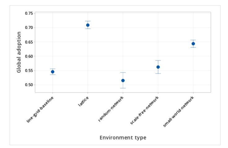
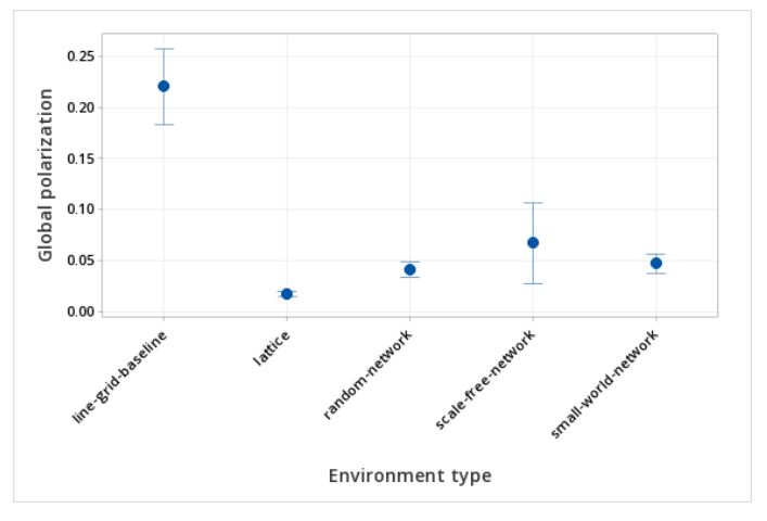
In both the first and second analysis, the only variable changed was environment type (line grid baseline and four networks) and the associated change made to the neighborhood and local observer view for the networks. All the other variables were fixed. When considering environment types consisting of both the line grid and networks, an analysis of variance indicated that the environment type explained 53% of the variation of adoption and 40% of the variation of global polarization. Details of these analyses are in the the (Appendix) (Hypothesis Two: Supplementary Information). Local polarization was not examined in this analysis, given that the random, small-world and scale-free networks did not consider a grid component, from which the local polarization calculation is derived.
Limiting the environment type to networks enabled further analysis to understand which network characteristics contribute to explaining adoption and polarization. The model is shown in Equation 5.
| \[ \begin{split} Global Adoption_{networks}= f(average\hspace{4pt} eigenvector centrality,\hspace{4pt}\\ average\hspace{4pt} betweeness\hspace{4pt} centrality,\\ average \hspace{4pt}clustering\hspace{4pt} coefficient,\\mean\hspace{4pt} path \hspace{4pt}length, \hspace{4pt}modularity) \end{split}\] | \[(5)\] |
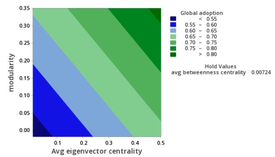
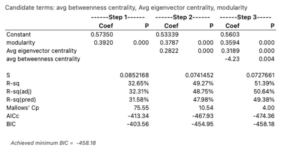
Analysis of variance was used to understand which variables statistically explained adoption variability. The factors modularity and average eigenvector centrality were the most significant factors. With all the variables at default values, the network characteristics explained 51% of adoption variation within network environments (Table 7). Using a similar analysis, the polarization result was not significant (adjusted r-squared of 2%), meaning that the network characteristics did not have a significant impact on polarization when other factors were held constant.
| Source | DF | Contribution | F-Value | P-Value |
|---|---|---|---|---|
| Average betweeness centrality | 1 | .81% | 8.54 | 0.004 |
| Average eigenvector centrality | 1 | 24.16% | 75.55 | 0.000 |
| Modularity | 1 | 26.41% | 106.49 | 0.000 |
| Error | 196 | 46.61% | ||
| Total | 199 |
Given the results above, eigenvector centrality and modularity both contribute in a positive direction as shown in the contour plot in Figure 7.
H3: Impact of all variables on adoption and polarization
The last analysis explained about 50% of the variation in adoption when only varying the environment type, motivating an additional study to test the sensitivity of all the variables to understand the role other factors may have to explain adoption and polarization. The full experiment in Table 6 was run with the environment type as a categorical variable, including line grid baseline. The model used is described in Equation 6.
| \[ \begin{split} Global \hspace{2pt} adoption = f(b,\hspace{4pt} \lambda,\hspace{4pt}observer\hspace{3pt} view,\hspace{4pt} f,\hspace{4pt} environment \hspace{3pt}type,\hspace{4pt} \lambda \hspace{4pt} b ) \end{split}\] | \[(6)\] |
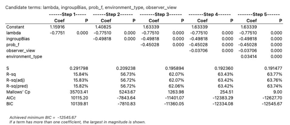
With this approach, 64% of the adoption variability was explained (adjusted r-squared). The most significant variables were the outgroup bias factor (b) at 41% explained, and the frequency dependency factor (\(\lambda\)) at 16% explained and neighborhood to non-neighborhood proportion (f) at 5%. The remaining factors, while significant, accounted for the rest of the explained percent in this order: observer view (local/global), and environment type. With the inclusion of other variables, the environment type diminished in importance in explaining adoption. The results are in Table 9. Given the adoption equation, the interaction of b and \(\lambda\) was included in the analysis; however, including the interaction effect created multicollinearity with high variance inflation factors (greater than 10) for the outgroup factor and the interaction term, so the interaction term was removed, despite contributing to 10% higher percent explained. The correlation between the outgroup factor and the interaction term was .89, which shows additional evidence of potential multicollinearity. The variance unexplained i.e. percent error, at 36%, was due to the stochastic and non-linear characteristics of the experiment that added noise: generating a new network with each replication, random location of the seeds, the random assignment of groups to agents, and the probability calculation itself.
| Source | DF | Contribution | F-Value | P-Value |
|---|---|---|---|---|
| Environment type | 4 | .34% | 63.39 | 0.000 |
| Outgroup bias, \(\textit{b}\) | 1 | 40.89% | 30,469.58 | 0.000 |
| Observer view | 1 | 1.36% | 1,011.73 | 0.000 |
| Frequency dependence, \(\lambda\) | 1 | 15.84% | 11,801.08 | 0.000 |
| Neighborhood probability, \(\textit{f}\) | 1 | 5.34% | 3,982.71 | 0.000 |
| Error | 26,991 | 36.23% | ||
| Total | 26,999 |
Considering all factors, global polarization had a lower percent explained at 29% compared to adoption. The global polarization analysis of variance details are in the Appendix.
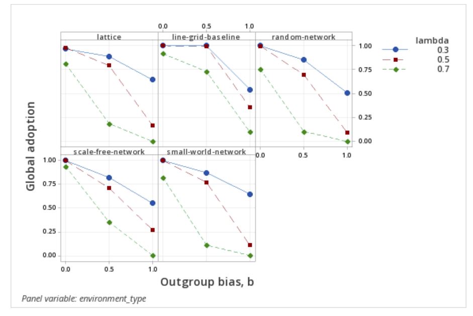
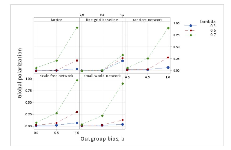
Given the impact of frequency dependence and the outgroup factor, b, the network structures amplify the frequency effects by lowering adoption and increasing polarization compared to the line grid baseline as shown in Figures 8 and 9. With frequency dependency, \(\lambda\), at 0.7, adoption declines precipitously, and polarization increases substantially with increases in the outgroup factor. These effects are more muted in the line grid baseline, but are directionally the same. A possible reason for this effect at \(\lambda\) = .7 is that the baseline case has perfect mixing and a higher number of observations. These two effects change the dynamics of the outgroup factor over its relevant range of values. These effects are potentially amplified due to the exponential nature of \(\lambda\) which increases in-group adoption at higher values of \(\lambda\). Polarization is in turn impacted by this effect on adoption as differences grow between in-group and out-group adoption.
Discussion
Adoption and polarization were different in a lattice network versus a line grid baseline
Testing the first hypothesis showed that overlaying a lattice network environment for adoption with outgroup effects while keeping all other parameters at default levels led to a higher level of global adoption and a slightly lower level of polarization (Table 6). However, for adoption, as shown in Figure 8, this is only when the frequency dependence factor, \(\lambda\), is at the default value of 0.3. At higher values of frequency dependence (0.5 and 0.7), the adoption percent is lower when the full outgroup effect, b, is equal to one (Figure 8). Similarly, for polarization, when the frequency dependence, \(\lambda\), is 0.3, the line grid baseline shows higher polarization; however, when the frequency dependence goes to 0.5 or 0.7, global polarization is at parity or higher for the network environments than for the line grid baseline with one exception for the small world network (Figure 9).
Local polarization, the average polarization within each grid square, was much lower in the lattice network than the line grid baseline (Table 6). This may be due to modifying the observation mechanism to accommodate the network characteristics of neighborhood and distance for defining the local observer view. The links were applied to the line grid baseline based on the radius from the given agent and the groups within a grid square were not randomized (see Figure 2), resulting in many of the agents’ neighborhoods and local observer views to be linked to their own group. In the line grid baseline environment, the clique structure and the local observer view created higher mixing between the groups during the evaluation process which may explain the higher level of local polarization. The linking of like-group agents within a grid square is consistent with dynamic models of segregation where groups sort into neighborhoods with similar characteristics (Schelling 1971). The smaller observer view is also consistent with Centola & Macy (2007) that a lower number of sources influencing adoption is more important that the number of exposures, or in this case observations. The lower global and local polarization effect overall is important so that projecting potential resistance to innovation is not unnecessarily overstated.
The implication of this finding is that using an accurate value of the frequency dependence factor, \(\lambda\), (imitation factor) is critical for accurately projecting overall adoption or polarization on a network. Additionally, while introducing the network environment to the model produced different levels of adoption and polarization, directionally it was consistent, given the equations and model structure. Since networks are known social structures for adoption processes (Rand & Rust 2011), this may encourage use of the model as a more viable option for forecasting adoption with outgroup effects. Finally, given the sensitivity of adoption and polarization to the value of the frequency dependence factor with full outgroup effects, the use of an exponential factor, \(\lambda\), may be an area to explore further with a more conventional expression of the imitation factor such as that in Bass (1969) or Rand & Rust (2011), which uses linear coefficients versus an exponential factor for modeling innovator and imitator adoption.
The small world and lattice networks had higher adoption levels than the other environments tested
The second hypothesis test examined the outgroup effect on various networks beyond the modified lattice network keeping all other factors at default levels (Table 7). The skew factor was equalized to 0.5 in all cases to enable a consistent evaluation, given that local polarization effects were not meaningful for the other network environments. For adoption, the lattice network and the small world network had the highest adoption compared to the three other environment types.
Both the small world and lattice networks share the characteristics of random connections across the environment. The implication is that adoption is higher in environments with connections outside of their immediate neighbors. The higher adoption from these structures is consistent with Granovetter (1973) showing the role of random connections in social networks. Additionally, the model is consistent with Centola & Macy (2007), in that the adoption decision is based on social affirmation from multiple sources in the network structure, not just the random connections alone. In a social context, these may be connections from serving in the military, distant family relationships or from college friendships that extend beyond immediate neighbors.
Given the differences in adoption between the network types (a subset of the variable, "Environment type"), understanding the type of social network will enable a more accurate adoption projection for emerging innovations when outgroup effects are present. Lacking the full knowledge of the network structure and gaining an understanding of a few crucial metrics will contribute to ensuring the efficacy of the model, which is discussed next.
Modularity and average eigenvector centrality impacted adoption the greatest within network environments
Holding other parameters at default levels, the two most significant network characteristics influencing adoption are modularity and average eigenvector centrality. Examining this effect statistically showed these two factors as having the largest contribution to adoption variation (Table 8). Figure 7 shows that as both modularity and average eigenvector centrality increase, adoption also increases. To the extent that the network structure is driven by group membership compared to a random structure (modularity), adoption tends to be higher. For example, if the network relationships are from work, church, or similar political affiliation, and the group takes a position on adopting or not adopting an innovation, then there is a higher likelihood of impacting the rate of adoption. Vaccination decisions may be an example where getting vaccinated was associated with political affiliations and information emanating from political parties (Ivory et al. 2021).
The eigenvector centrality is highest for the lattice and small world networks, which also had the highest adoption rates. Eigenvector centrality considers not only the number of neighbors a node has, but also the importance of those connected nodes (Newman 2018). The rewiring in both the lattice and small world networks is likely the reason eigenvector centrality plays a role in greater adoption. The rewired connections are important in spreading the adoption to other areas of the network through small world effects. An example in decentralized finance may be disparate parties in different countries or socio-economic status linked by their use of a crypto currency as a medium of exchange.
A limitation of this analysis is that the network metrics were not orthogonally tested as a designed experiment, given that the characteristics measured are the result of generating each network. The statistical analysis should be considered directional i.e. that about half of the adoption variation can be explained by network characteristics. While in this study the network type and the associated metrics were examined, further analysis may consider outgroup effects related to social diffusion from the number of community dimensions, the degree of homophily and consolidation, and network bridge width (Centola 2015).
On networks, higher frequency dependence hinders adoption and increases polarization when outgroup effects are present
The last experiment examined the effect of all the variables on adoption. Consistent with Smaldino et al. (2017), outgroup aversion is shown to hinder adoption. On networks, adoption is hindered somewhat more (Figure 8) with higher outgroup aversion and higher frequency dependence. However, in the case of polarization, our results differ from Smaldino et al. (2017) with network environments showing more amplified polarization as frequency dependence and the outgroup factors are increased (Figure 9). The equations for the adoption decision show that increasing the frequency dependency factor increases the probability of adoption; however, higher outgroup factor discounts this effect. The cause may also be related to the observer view mechanism, or the lower effective degree of each network compared to the line grid baseline. Higher polarization sensitivity may also be due to the interplay between the proportion of neighborhood vs. non-neighborhood observer view (probability f) and the network. In summary, the network environments amplified the effect of lower adoption and higher polarization with increasing outgroup factor and at higher frequency dependency.
Higher level of frequency dependence or imitation effects can drive higher polarization when outgroup effects are present. For innovations such as vaccines, this may be why non-adopters or anti-vaxers can dominate a local area as the imitation effect works against adoption when the outgroup non-adopters are dominant. For decentralized finance, a critical mass of suppliers and customers would need to have adopted to crypto currency in order to facilitate widespread adoption, irrespective of outgroup effects.
Due to the stochastic nature of network generation, placement of the seed adopters, the randomness from the local and global observations and the adoption probability itself, 100% of adoption variation is not able to be explained. These elements all create random errors to mimic circumstances encountered in the real world. Additionally, the system simulated is an inherently non-linear system whereas the statistical analysis assumes a general linear model (GLM).
Conclusion
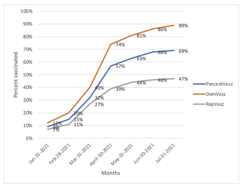
These findings explain how network structure can amplify adoption and polarization with outgroup effects by including network environments as the medium for innovation diffusion. For emerging innovations, effective use of the model requires accurate assumptions for the network characteristics, the likelihood of imitation effects and assumptions about the presence of groups whose association with an innovation may inhibit adoption in the outgroup. While this research focused on isolating the addition of network effects, with default parameters and retaining a core model of adoption with outgroup effects, the model can be extended further by revisiting the equation for the adoption likelihood and empirically validating the model to reflect actual outgroup behavior to evolve the model further. Vaccine hesitation is a good candidate, given the amount of data available. Figure 10 shows the potential outgroup effect of vaccines from 2021 , with distinct differences in percent vaccinated by political affiliation. The difference between vaccination rates by party affiliation (or group) is 42%. The models from this study may enable explaining a portion of this effect.
Future analysis and extensions include identifying empirical examples related to climate change innovations, vaccination hesitation or decentralized finance where adoption may be hindered by outgroup effects to calibrate the outgroup factor and the frequency dependence. For vaccination adoption, the model might test the hypothesis that political affiliation may be one of several significant predictors of vaccination adoption behavior. Data from elections by county merged with census data regarding other factors such as socio-economic factors, availability of healthcare or population density may enable understanding how much the outgroup effect impacts behavior. The network set-up of agents may reflect the actual geo-spatial distribution of populations with various characteristics. Adding to this, the next iteration of the model may replace the frequency dependence term with the innovator and imitation terms (Bass 1969; Rand & Rust 2011) or a social learning model of conformity (Henrich & Boyd 1998). Before making a decision, agents form opinions of what they are planning to do and the model could consider the role of information sources, opinion dynamics and extremism that influence and converge group attitudes toward an innovation along the lines of Deffuant et al. (2005). As actual social networks are considered, additional network metrics or structural characteristics may have an impact on adoption (e.g., assortativity, communities, network bridge width). Incentives, or mandates may play a role for the model, including potential amplification of polarization for mandates or penalties. Where there is not opinion convergence, perhaps group membership can be considered in terms of a heterogenous “degree” vs. just a binary group one vs. group two. For example, there may be enthusiastic group members and more passive or neutral members. Finally, all these concepts might be tested or validated with the the development of a survey instrument to randomly distribute in a community to understand the strength of group identification and its role for adopting emerging innovations.
Appendix: Supplementary Information
Network information
| Environment | Average Degree | Nodes | Edges | Average Betweenness Centrality | Average Clustering Coefficient | Density | Average Eigenvector Centrality | Mean Path Length | Modularity |
| Lattice Network | 6.11 | 1764 | 5390 | 0.00614 | 0.535 | 0.0035 | .158 | 11.9 | .348 |
| Random Network | 6.00 | 1764 | 5292 | .0112 | 0.545 | .0034 | .0108 | 20.78 | 0.000 |
| Scale-free Network | 5.99 | 1764 | 5286 | 0.00152 | 0.0217 | 0.0034 | 0.0366 | 3.68 | 0.000 |
| Small-world Network | 6.00 | 1764 | 5292 | 0.0101 | 0.583 | 0.0034 | 0.379 | 18.77 | 0.000 |
Sample Runs
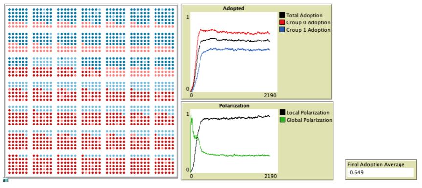
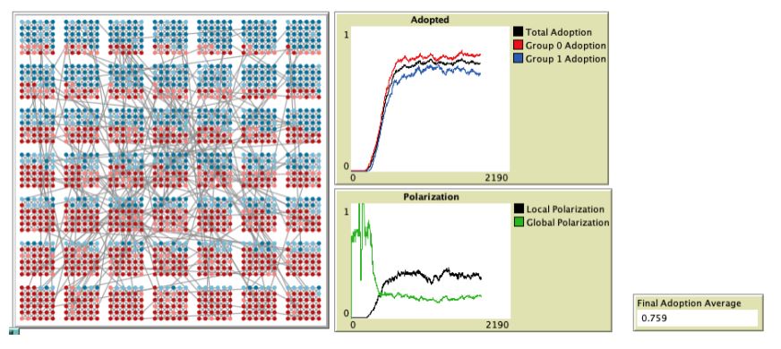
Figure 11 shows a sample run graph for the line grid baseline and Figure 12 shows a sample run for the lattice network, both with default parameter values. The sample run graphs are consistent with the results in Table 6 showing higher adoption, lower global polarization and lower local polarization for the lattice network compared to the line grid baseline.
Local observer view example
With \(f = .7\) and degree an average of six, the number of observations to sample for the local observer view is shown in the calculation below:
| \[0.7 = \dfrac{6}{local + 6}\] | \[(7)\] |
| \[local = \dfrac{1.8}{.7}= 2.57\hspace{4pt} observations\] | \[(8)\] |
In this case, 2.57 would be rounded to 3 and three observations from the pool of nodes that are two links out from the selected node would be taken. The ratio of neighborhood to non-neighborhood is then preserved at 6/9 = .66 or rounded to .7. This approach works well for all the network types, except for when the degree is 1 or 2. In this case the neighborhood would consist of the links around the node and then the local view would default to be the degree of the node. In this case, such normalization is justified from the strength of weak ties theory (Granovetter 1973). This is mostly an issue in the scale free network.
H2: Supplementary Information
| Environment Type | N | Mean | Grouping |
|---|---|---|---|
| Line grid baseline | 50 | 0.694 | A |
| Lattice network | 50 | 0.154 | B |
| Random network | 50 | 0.148 | B |
| Small-world network | 50 | 0.140 | B |
| Source | DF | Adj SS | Adj MS | F-Value | P-Value |
|---|---|---|---|---|---|
| Environment type | 4 | 1.270 | 0.318 | 71.91 | 0.00 |
| Error | 245 | 1.082 | 0.00442 | ||
| Total | 249 | 2.352 |
| Source | DF | Adj SS | Adj MS | F-Value | P-Value |
|---|---|---|---|---|---|
| Environment type | 4 | 1.322 | 0.330 | 43.41 | 0.000 |
| Error | 245 | 1.866 | 0.00762 | ||
| Total | 249 | 3.188 |
| Source | DF | Adj SS | Adj MS | F-Value | P-Value |
|---|---|---|---|---|---|
| Environment type | 4 | 12.0267 | 3.007 | 3,466.83 | 0.000 |
| Error | 245 | 0.2125 | 0.00087 | ||
| Total | 249 | 12.2392 |
H3: Supplementary Information
| Source | DF | Seq SS | Contribution | Adj SS | Adj MS | F-Value | P-Value |
|---|---|---|---|---|---|---|---|
| Lambda | 1 | 155.94 | 8.28% | 155.94 | 155.94 | 3147.76 | 0.000 |
| Outgroup bias, b | 1 | 317.78 | 16.87% | 317.78 | 317.78 | 6,414.38 | 0.000 |
| Probability f | 1 | 18.91 | 1% | 18.91 | 18.91 | 381.65 | 0.000 |
| Skew, Q | 1 | 10.76 | 0.57% | 10.76 | 10.76 | 217.22 | 0.000 |
| Environment Type | 4 | 42.63 | 2.26% | 42.63 | 10.658 | 215.14 | 0.000 |
| Observer view | 1 | 0.21 | 0.01% | 0.21 | 0.212 | 4.27 | 0.039 |
| Error | 26990 | 1,337.11 | 71.00% | 1,337.11 | 0.05 | ||
| Total | 26,999 | 1,883.34 | 100.00% | ||||
| Model Summary: R-sq = 29\(\%\), R-sq(adj)=28.98\(\%\) | |||||||
References
BARABASI, A. L. (2016). Network Science. Cambridge: Cambridge University Press.
BARABASI, A. L., & Albert, R. (1999). Emergence of scaling in random networks. Science, 286(5439), 509–512.
BASS, F. M. (1969). A new product growth for model consumer durables. Management Science, 15(3), 215–227. [doi:10.1287/mnsc.15.5.215]
BERGER, J., & Heath, C. (2007). Where consumers diverge from others: Identity signaling and product domains. Journal of Consumer Research, 34(2), 121–134. [doi:10.1086/519142]
BERGER, J., & Heath, C. (2008). Who drives divergence? Identity-signaling, outgroup dissimilarity and the abandonment of cultural tastes. Journal of Personality and Social Psychology, 95(3), 593–607. [doi:10.1037/0022-3514.95.3.593]
BORGATTI, S. P., Mehra, A., Brass, D. J., & Labianca, G. (2009). Network analysis in the social sciences. Science, 323, 892–895. [doi:10.1126/science.1165821]
BOYD, R., & Richerson, P. J. (1988). Culture and the Evolutionary Process. Chicago, IL: University of Chicago Press.
BURNHAM, K. P., & Anderson, D. R. (2004). Multimodel inference: Understanding AIC and BIC in model selection. Sociological Methods & Research, 33(2), 261–304. [doi:10.1177/0049124104268644]
CENTOLA, D., & Macy, M. (2007). Complex contagions and the weakness of long ties. The American Journal of Sociology, 113(3), 702–734. [doi:10.1086/521848]
DEFFUANT, G., Huet, S., & Amblard, F. (2005). An individual-based model of innovation diffusion mixing social value and individual benefit. American Journal of Sociology, 110(4), 1041–1069. [doi:10.1086/430220]
DUNBAR, R. I. (1992). Neocortex size as a constraint on group size in primates. Journal of Human Evolution, 469–493. [doi:10.1016/0047-2484(92)90081-j]
ERDOS, P., & Renyi, A. (1960). On the evolution of random graphs. Publi. Math. Inst. Hung. Acad. Sci, 17–60.
FREEMAN, L. C. (2000). Social network analysis: Definition and history. In A. E. Kazdin (Ed.), Encyclopedia of Psychology (Vol. 7, pp. 350–351). Oxford: Oxford University Press. [doi:10.1037/10522-151]
GARIBAY, I., Mantzaris, A. V., Rajabi, A., & Taylor, C. E. (2019). Polarization in social media assists influencers to become more influential: Analysis and two inoculation strategies. Scientific Reports, 9(1), 1–9. [doi:10.1038/s41598-019-55178-8]
GARIBAY, I., Oghaz, T. A., Yousefi, N., Mutlu, E., Schiappa, M., Scheinert, S., Anagnostopoulos, G. C., Bouwens, C., Fiore, S. M., Mantzaris, A., Murphy, J. T., Rand, W., Salter, A., Stanfill, M., Sukthankar, G., Baral, N., Fair, G., Gunaratne, C., Hajiakhoond, N. B., Jasser, J., Jayalath, C., Newton, O., Saadat, S., Senevirathna, C., Winter, R. & Zhang, X. (2021). Deep agent: Studying the dynamics of information spread and evolution in social networks. Proceedings of the 2019 International Conference of The Computational Social Science Society of the Americas. [doi:10.1007/978-3-030-77517-9_11]
GOLDENBERG, J., Han, S., Lehmann, D. R., & Hong, J. W. (2009). The role of hubs in the adoption process. Journal of Marketing, 73(2), 1–13. [doi:10.1509/jmkg.73.2.1]
GOLDENBERG, J., Libai, B., Moldovan, S., & Muller, E. (2001). Talk of the network: A complex systems look at the underlying process of word-of-mouth. Marketing Letters, 12(3), 211–233. [doi:10.1023/a:1011122126881]
GOLDENBERG, J., Libai, B., Moldovan, S., & Muller, E. (2007). The npv of bad news. International Journal of Research in Marketing, 24(3), 186–200. [doi:10.1016/j.ijresmar.2007.02.003]
GRANOVETTER, M. S. (1973). The strength of weak ties. American Journal of Sociology, 78(6), 1360–1380. [doi:10.1086/225469]
GRIMM, V., Polhill, G., & Touza, J. (2017). Documenting social simulation models: The ODD protocol as a standard. In B. Edmonds & R. Meyer (Eds.), Simulating Social Complexity. Berlin Heidelberg: Springer. [doi:10.1007/978-3-319-66948-9_15]
HAGBERG, A., Swart, P., & S Chult, D. (2008). Exploring network structure, dynamics, and function using NetworkX. Los Alamos National Lab.(LANL), Los Alamos, NM (United States)
HENRICH, J., & Boyd, R. (1998). The evolution of conformist transmission and the emergence of between-group differences. Evolution and Human Behavior, 19(4), 215–241. [doi:10.1016/s1090-5138(98)00018-x]
IVORY, D., Lauren, L., & Gebeloff, R. (2021). Least vaccinated in US counties have something in common: Trump voters. The New York Times. Available at: https://www.nytimes.com/interactive/2021/04/17/us/vaccine-hesitancy-politics.html.
KEISLING, E., Gunther, M., Stummer, C., & Wakolbinger, L. M. (2012). Agent-based simulation of innovation diffusion: A review. Central European Journal of Operations Research, 20, 183–230.
KLEIN, E. (2020). Why We’Re Polarized. New York, NY: Simon & Schuster.
MILGRAM, S. (1967). The small world problem. Psychology Today, 2(1), 60–67.
MILLER, B. G., Garibay, I., & Hoekstra, R. (2021). An innovation case study: A process, practice and learning perspective from a large hospitality and entertainment business. Proceedings of IIE Annual Conference. Available at: https://www.proquest.com/scholarly-journals/innovation-case-study-process-practice-learning/docview/2560890651/se-2?accountid=10003
MINITAB. (2021). Minitab. Available at: https://app.minitab.com
MORENO, J. L. (1934). Who Shall Survive? New York, NY: Beacon House.
MUTLU, E., & Garibay, I. (2021). The degree-dependent threshold model: Towards a better understanding of opinion dynamics on online social networks. [doi:10.1007/978-3-030-77517-9_7]
NEWMAN, M. (2006). Modularity and community structure in networks. Proceedings of the National Academy of Sciences, 103(23), 8577–8582. [doi:10.1073/pnas.0601602103]
NEWMAN, M. (2018). Networks. Oxford: Oxford University Press.
RAND, W., & Rust, R. T. (2011). Agent-based modeling in marketing: Guidelines for rigor. International Journal of Research in Marketing, 28(3), 181–193. [doi:10.1016/j.ijresmar.2011.04.002]
ROGERS, E. M. (2003). Diffusion of Innovations. New York, NY: Free Press.
SAID, L. (2021). More in u.s. Vaccinated after delta surge, fda decision. https://https://news.gallup.com/poll/355073/vaccinated-delta-surge-fda-decision.aspx. Accessed: 2021-09-29.
SCHELLING, T. C. (1971). Dynamic models of segregation. Journal of Mathematical Sociology, 1(2), 143–186.
SIMMEL, G. (1922). The Web of Group-Affiliations. New York, NY: Free Press.
SIMMEL, G. (1964). The Sociology of Georg Simmel. New York, NY: Free Press.
SMALDINO, P. E., Janssen, M. A., Hillis, V., & Bednar, J. (2017). Adoption as a social marker: Innovation diffusion with outgroup aversion. The Journal of Mathematical Sociology, 41(1), 26–45. [doi:10.1080/0022250x.2016.1250083]
TARDE, G. (1903). The Laws of Imitation. New York, NY: H.Holt.
WASSERMAN, S., & Faust, K. (1994). Social Network Analysis. Cambridge University Press.
WATTS, D. J., & Strogatz, S. H. (1998). Collective dynamics of “small-world” networks. Nature, 393(6684), 440–442. [doi:10.1038/30918]
WILENSKY, U. (1999). NetLogo. Avialable at: http://ccl.northwestern.edu/netlogo/
ZHANG, H., & Vorobeychik, Y. (2019). Empirically grounded agent-based models of innovation diffusion: A critical review. Artificial Intelligence Review, 52, 707–741. [doi:10.1007/s10462-017-9577-z]