Scientific Disagreements and the Diagnosticity of Evidence: How Too Much Data May Lead to Polarization

Matteo Michelini; Javier Osorio; Wybo Houkes; Dunja Šešelja; Christian Straßer

doi:10.18564/jasss.5113

Introduction

Scientific disagreements and controversies are commonly considered crucial for the advancement of scientific ideas (Longino 2002, 2022; Solomon 2007). Yet, they may also lead to fragmented or polarized scientific communities, with scientists unable to reach consensus on issues that may be of social relevance and pertinent to policy guidance. While the exchange of information across a scientific community can help to bring everyone on the same page, disagreement may persist even if evidence is shared, as shown for instance by the limited success of so-called consensus conferences (Stegenga 2016).

One possible explanation for such persistent disagreements is that scientists differ in how significant they consider the same experimental result, i.e. they differ in how diagnostic they take the results to be relative to a given research hypothesis. The reason is that scientists may interpret experiments on the basis of different background assumptions, methodologies or theoretical commitments. In a well-known case in the history of science, Ignaz Semmelweis observed that the incidence of puerperal fever could be drastically cut by washing his hands. Semmelweis’ observations conflicted with the established scientific opinions of the time and his ideas were rejected by the medical community. While Semmelweis assigned a high diagnostic value to his observations regarding the hypothesis that handwashing reduced the mortality ratio, the scientific community assigned a comparatively low value.

A related factor that might lead to persistent scientific disagreements is that scientists tend to learn and adjust their background beliefs and methods primarily through communication with like-minded peers. As a result, even if the community extensively shares available evidence, divergent ways of interpreting evidence may persist and contribute to persisting disagreements. Moreover, it raises the question whether the amount of available evidence in such a community impacts the emergence of polarization.

In this paper we develop an agent-based model (ABM) to examine the above ideas, viz.tackle the hypothesis that a scientific community can become polarized if scientists disagree on the diagnosticity of their experimental results in spite of fully sharing the available evidence. For this purpose, we study opinion dynamics in a community of Bayesian agents who are trying to determine whether to accept or reject a certain hypothesis. Throughout their inquiry, scientists are exposed to the same evidence and treat evidence as certain, but they assign different significance to the available evidence.

Our ABM is based on bandit models, commonly used in simulations of scientific communities (O’Connor & Weatherall 2018; Zollman 2007, 2010). In particular, agents (modeled as Bayesian updaters) face a one-armed bandit, representing a certain scientific hypothesis, and they try to determine whether to accept it or to reject it. Throughout their research, agents acquire evidence and exchange information about the diagnostic value (modeled in terms of the Bayes factor) that they ascribe to evidence. While the exchange of gathered evidence is modeled in terms of batches of data that may vary in size, the exchange concerning the diagnostic value of evidence is modeled in terms of the bounded confidence model (Douven & Hegselmann 2022; Hegselmann & Krause 2002, 2006). In this way we represent scientists who have a ‘bounded confidence’ in the opinions of their peers, so that they exchange their views on the diagnostic force of evidence only with those who have sufficiently similar beliefs about the world as they do.

Our results show that an initial disagreement on the diagnostic value of evidence can, but does not necessarily, lead to polarization in a scientific community, depending on the sample size of the performed studies and the confidence interval within which scientists share their opinions. These findings shed light on how different ways of interpreting evidence affect polarization in scenarios in which no detrimental epistemic factors are present, such as biases, deceptive information, uneven access to evidence, uncertainty about evidence etc.

The paper is structured as follows. We start with the Theoretical Background where we provide a brief overview of related models, focusing on those that study scientific disagreements and polarization. Next, in the Model Description we present our ABM in terms of the ODD protocol (Grimm et al. 2020). In the Results section we present our main findings, and we perform an uncertainty and sensitivity analysis. The Discussion situates our results into the broader literature on ABMs studying opinion dynamics in epistemic communities, while Conclusion addresses some open lines for further research. The two appendices present a mathematical analysis of one aspect of our model and a more detailed description of the model in the ODD format.

Theoretical Background

Opinion dynamics in truth-seeking communities has long been studied by means of computer simulations. From the early work of Hegselmann & Krause (2006), following their pioneering (2002) model as well as related work by Deffuant et al. (2002), a range of ABMs have been used to examine conditions under which a community of rational agents may polarize.¹ While Hegselmann & Krause (2006) showed that polarization can emerge if some agents form beliefs by disregarding evidence from the world and by instead considering only what they learn from others with sufficiently similar views, others have looked into communities in which all agents form their beliefs on the basis of evidence coming from the world. For example, Singer et al. (2017) show how polarization can emerge in a community of deliberating agents who share reasons for their beliefs, but who use a coherence-based approach to manage their limited memory (by forgetting those reasons that conflict with the view supported by most of their previous considerations). Olsson (2013) demonstrates how polarization can emerge over the course of deliberation if agents assign different degrees of trust to the testimony of others, depending on how similar views they hold. O’Connor & Weatherall (2018) show how a community of scientists who share not only their testimony, but unbiased evidence, can become polarized if they treat evidence obtained by other scientists, whose beliefs are too different from their own, as uncertain. Moreover, ABMs examining argumentative exchange such as those by Mäs & Flache (2013) and Kopecky (2022) demonstrate how a community of deliberating agents can polarize due to specific argumentative dynamics.

In this paper, we explore similar scenarios to those outlined above with one substantial difference: agents can assign different diagnostic values to the evidence in view of which they evaluate the hypotheses at stake. In scientific inquiry, a collection of data is evidence for a given hypothesis insofar as there is an epistemic background that makes it possible to trace a connection between the data and the hypothesis (Longino 2002). For this reason, “researchers must combine their theoretical viewpoint with the questions at hand to evaluate whether a particular data set is, in fact, evidential” (Morey et al. 2016). In other words, the different ways in which evidence is interpreted feed back into how strong a subject may believe in a given hypothesis. The fact that the diagnosticity of evidence is relative to the epistemic background of a reasoner is familiar from non-scientific contexts: while the observation of a wet street may convince one person that it rained, it will not convince another person who assumes that streets tend to be regularly cleaned. In the context of scientific reasoning, background assumptions and methodological standards may similarly affect the interpretation of evidence, and may in turn lead scientists to different beliefs and different preferred theories. Therefore, the diagnostic value of a piece of evidence is at the core of scientific disagreements and their structural dynamics.

As mentioned above, we model our agents as Bayesian reasoners. This means that their beliefs are represented by probability functions. After receiving a piece of evidence $e$ the belief of an agent in a hypothesis $H$ is updated according to Bayes’ theorem to obtain the posterior belief $P(H\mid e)$ as a function of her prior beliefs. The diagnosticity of $e$ plays a central role for this, as can be seen in the following reformulation of Bayes’ theorem in terms of odds:

\[ \underbrace{\frac{\overbrace{\color{red}{P(H\mid e)}}^{\substack{\mbox{posterior}\\\mbox{belief in $H$}}}}{{P(\neg H \mid e)}}} _{\substack{\mbox{posterior}\\\mbox{odds}}} \qquad == \qquad \underbrace{\frac{ \overbrace {P(e\mid H)} ^{\substack{\mbox{how predictive}\\\mbox{is $H$ of $e$?}}} } {{P(e\mid \neg H)}}} _{\substack{\mbox{likelihood ratio} \\\mbox{resp.}\\\mbox{diagnostic}\\\mbox{value}}} \quad \times \quad \underbrace{ \frac{ \overbrace{P(H)}^{\substack{\mbox{prior} \\ \mbox{belief in $H$}}}}{P(\neg H)}}_{\substack{\mbox{prior}\\\mbox{odds}}}\]

\[(1)\]

Clearly, the posterior odds for $H$ is, among others, a function of the prior odds for $H$. Additionally, it is a function of the likelihood ratio, also known as the Bayes factor (Morey et al. 2016). It determines the diagnosticity of the given evidence $e$ for $H$ (Hahn & Hornikx 2016). Consider our example from above with an agent observing the wet streets under the hypothesis that it rained. For her, $P(e \mid \neg H)$ will be very low and $P(e \mid H)$ very high, leading to a high diagnosticity of the wet streets for rain. In contrast, our second agent, who assumes the streets are regularly cleaned, may have a similar high $P(e\mid H)$, but also a high $P(e\mid \neg H)$ in view of his assumption of an alternative explanation. The diagnosticity he assigns to $e$ for $H$ will be comparatively low. In general, a diagnostic value above (resp. below) 1 indicates that $e$ is positively (resp. negatively) diagnostic of $H$, while if it is 1 $e$ is statistically irrelevant for $H$.

Taking this point of departure, we now introduce our model.

Model Description

In this section we present our model in accordance with the ODD protocol (Grimm et al. 2020). We focus on selected elements, to provide a clear overview of the model without getting lost in technicalities. The full description of the model in the ODD format can be found in the Appendix B. The code is available at: https://www.comses.net/codebase-release/3b729700-837d-4d62-a41c-366a37ced7e5/.

Purpose and main pattern of the model

The present model is an abstract ABM designed for theoretical exploration and hypotheses generation. As mentioned in the Introduction, our main aim is to explore the relationship between disagreement over the diagnostic value of evidence and the formation of polarization in scientific communities.

The model represents a scientific community in which scientists aim to determine whether hypothesis $H$ is true, where we assume that agents are in a world in which $H$ is indeed true. To this end, scientists perform experiments, interpret data and exchange their views on how diagnostic of $H$ the obtained evidence is. Our model captures two notions of disagreement: on the one hand, a disagreement on the hypothesis $H$, and on the other hand, a disagreement on the diagnostic value of value of evidence for $H$.

Entities, state variables

The model features two different entities: the agents, who represent the scientists, and the environment (or observer), which describes the scientific problem at stake and keeps track of time. In every turn of the model, the scientific community gathers a new piece of evidence about the disputed hypothesis $H$. Each piece of evidence is fully shared and registered in the state variable evidence of the environment. The variable collects all the results up to that point and hence represents the state of the art concerning the evidence for $H$. In addition, the environment also keeps track of the time, i.e. the number of steps that have been performed up to that point. The scientists are characterized by the diagnostic value they assign to evidence and their degree of confidence in hypothesis $H$, which are tracked by two state variables.² When $\textit{agent-belief} > 0.99$ the agent fully supports $H$, whereas if $\textit{agent-belief} < 0.01$, the agent fully rejects $H$. The state-variables of scientists and environment are summarized in Tables 1 and 2 respectively.

**Table 1:** State Variables for Environment.
Variable	Variable-Type	Meaning
ticks (built-in Netlogo function)	integer, dynamic	the number of steps performed, which represents the passing of time
evidence	array of integers, dynamic	the number of successes obtained in the previous experiments over a certain number of trials (until the one observed in the present step. See the notation for ones in Paragraph 3.14)

**Table 2:** State Variables for Each Scientist.
Variable	Variable-Type	Meaning
agent-belief	$[0,1]$, dynamic	the probability an agent assigns to hypothesis $H$
agent-diag-value	$[0,1]$, dynamic	the diagnostic value an agent assigns to the output $1$ of a data point of an experiment (see Paragraph 3.15)

Process overview

Each step of the simulation has the following schedule.

A new piece of evidence becomes available in the scientific community, following the creation of an experiment submodel. The value is added to the state variable evidence of the environment.
Each agent executes the belief-update process based on the evidence that has been produced so far. Consequently, for each agent, the agent-belief variable is updated.
Agents go through the influence-each-other process. They update their agent-diag-value variable, based on the state variables of the agents they are connected with.
Every agent who changed the value for agent-diag-value in the last step reevaluates all available evidence. In particular, each agent executes the process of belief-update based on all the evidence that has been produced so far.
Ticks and observations are updated. The environment also checks if the stop condition is fulfilled.

The simulation stops when either

5000 steps have been performed or
every agent either fully supports $H$ or fully rejects $H$.

The second condition represents the effective termination of the debate, i.e.situation in which every scientist in the community has drawn a definitive conclusion on hypothesis $H$, and no further communication within the community will lead to further change. See Section Stability of the results for a justification of the first condition.

Our schedule is meant to represent the process of scientific inquiry, in which scientists continuously obtain potentially relevant evidence through experimentation, evaluate this evidence, and discuss with other members of the community on the basis of their background assumptions, i.e.diagnostic values. Step 1 represents the publication of new evidence, e.g., in a paper, which will be read and evaluated by all scientists in Step 2. Subsequently, Step 3 may be taken to represent a discussion which scientists could have at a conference.³ Finally, in Step 4 a scientist that has changed her mind with respect to the interpretation of evidence, reevaluates the evidence that the community has produced so far.

While the simulation runs, we collect the values for the state variables (Tables 1 and 2) of both environment and scientists. Finally, once the simulation has ended, we observe if the community has reached a correct consensus, a wrong consensus or polarization (intended as a state in which neither wrong consensus nor correct consensus are the case). Since our model is stochastic, we report the frequency of each of these outcomes for a certain parameter combination over 500 runs. In particular, we evaluate a certain parameter combination with respect to the frequency with which a consensus is generated.

Initialization

Initialization of the model is divided in two phases, corresponding to the setup of the scientific community (i.e.agents and the features of their behaviour) and the setup of the scientific problem the agents face. We start with the latter.

As mentioned in Section 3.1, the scientists face the problem of deciding whether or not hypothesis $H$ is true in the world in which they conduct their experiments (where we assume $H$ is true). To inform their decision, scientists perform experiments with a certain sample size. For each data point of the sample, they distinguish between an output of type $1$ and an output of type $0$ ($1$ and $0$ are mutually exclusive) as the outcome of the experiment. Such experiments are used to determine whether $H$ or $\neg H$ is more likely. Consequently, in the initialization, we fix the values of $P(1|H)$ and $P(1| \neg H)$.

We assume that $P(1|H) = 0.5$, i.e.if $H$ is the true state of the world (as it is), in the long run half of the data points will be of type $1$ and half of type $0$. Then, we assume that $P(1|\neg H) \in [0.55, 1)$, and we take the distance $d = P(1| \neg H) - P(1|H)$ to correspond to the difficulty of the problem at stake. The smaller $d$ is, the more likely $H$ and $\neg H$ are to yield a similar outcome, and the harder it is to decide which one of the two is responsible for the data on the basis of an experiment.

To set up the scientific community, we create $N$ agents, where $N$ can take up any value in $[5, 100]$. The state variable agent-belief for each agent is set to $0.5$, representing that scientists enter the debate without prior commitment to $H$ over $\neg H$. We assume that each agent is aware of the correct value for the probability of obtaining an output $1$ from $\neg H$ (that is $P_i(1|\neg H) = P(1|\neg H)$ for each $i$). Yet, at the same time, we consider the possibility for agents to assign to $P_i(1|H)$ a value different from $P(1|H)$. The value $P_i(1|H)$ is captured by the state variable agent-diag-value which is drawn for each agent from a uniform distribution $U (P(1|H) - \lambda, P(1|H) + \lambda)$, with $\lambda \in [0,0.5]$. This implies that

agents may have different diagnostic values, and that
agents may interpret evidence in a ‘wrong’ way.

Here, $\lambda$ represents the initial dispersion of agents’ background assumptions: we do not assume that agents assign the correct diagnostic value to evidence, but that it is very likely that the average computed over all the assigned diagnostic values is close to $P(1|H)$. In this, our model assumes a form of 'wisdom of the crowd' since the average value of the initial diagnostic values of all agents is closer to the real value than most of the individual initial values themselves.

Three other parameters are necessary to define the way agents interact and perform experiments (see Table 3), which will be explained in Section 3.13.

Submodels

Our model has three main submodels.

Creation of an experiment

At the beginning of each round, an experiment is performed and the result is made available to every agent. An experiment $e$ consists of a number $k$ of outputs of type ‘1’ (which we will call "ones", from now on) over a number of trials $n$: $k$ is drawn from a binomial distribution with number of trials $n = DP$, and probability $p = P(1|H)$ of producing a success. This representation of scientific experimentation has been used extensively in the philosophical approach to modelling scientific communities (O’Connor & Weatherall 2018; Zollman 2007). The number of trials for experiment $DP$ is a parameter in the interval $[5, 100]$.

Belief update

An agent may be presented with the outcomes of one or more experiments. In both cases, they update their belief through classical Bayesian updating. Let $e_1, \dots, e_m$ be the pieces of evidence the agent inspects and let $P_i^l(H)$ represent the belief before inspecting piece $e_{l+1}$. The value $P_i^l(H)$ corresponds to the state variable agent-belief before the update, and $P_i^{l+1}(H)$ to the state variable agent-belief after the update. The agent’s degree of belief after having observed $e_{l+1}$ is computed as follows:

\[P_i^{l+1}(H) = P_i^l(H |e_{l+1}) = \frac{P_i^l(H) \cdot P_i^l(e_{l+1}|H)}{P_i^l(e_{l+1})} = \frac{P_i^l(H) \cdot P_i^l(e_{l+1}|H)}{P_i^l(H) \cdot P_i^l(e_{l+1}|H) + P_i^l(\neg H) \cdot P_i^l(e_{l+1}|\neg H)}.\]

\[(2)\]

Consequently, if an agent inspects $m$ pieces of evidence: $P_i^m(H) = P_i^{m-1}(H | e_{m}) = P_i^{m-2}(H| e_{m} \land e_{m-1}) = ... = P_i^0(H | e_1 \land ... \land e_m)$. As we are dealing always with the same binomial distribution, $P_i^m(H)$ is equal to $P_i^0(H | E)$, where $E$ is an experiment with $k = k_1 + .... + k_m$ ones in $n = n_1 + ... + n_m$ trials. Importantly, in performing the update, the agent also employs $P_i^l(e_{l+1}|H)$ and $P_i^l(e_{l+1}|\neg H)$, which are respectively the likelihood that agent $i$ assigns to hypothesis $H$ of producing evidence $e_{l+1}$, and the likelihood that agent $i$ assigns to hypothesis $\neg H$ of producing evidence $e_{l+1}$. These two values can be computed as follows. If $e_{l+1}$ contains $k$ ones over $n$ trials, then:

\[P_i^l(e_{l+1}|H) = \binom{n}{k}\bigl(P_i(1|H))^k(1 - P_i(1|H)\bigr)^{n-k},\]

\[(3)\]

and

\[P_i^l(e_{l+1}|\neg H) = \binom{n}{k}\bigl(P_i(1|\neg H))^k(1 - P_i(1|\neg H)\bigr)^{n-k}.\]

\[(4)\]

Here, $P_i(1|H)$ corresponds to the value of the state variable agent-diag-value at the moment in which the update is performed. It represents the likelihood an agent assigns to obtaining a success in the experiment given that $H$ is true. By contrast, we take $P_i(1|\neg H) = P(1|\neg H)$ to be equal for all agents and consider it a parameter of the model: agents disagree over the relationship between $1$ and $H$, but not over the relationship between $1$ and $\neg H$.

Influence each other

After updating their beliefs on the basis of evidence, agents proceed to influence each other, by going through two phases:

choosing with whom to communicate (the ‘influencers’); and
updating the variable agent-diag-value based on the influencers’ values for the variable agent-diag-value.

Agent $i$ chooses the set $I_i$ of influencers such that $j \in I_i$ iff

\[(\textit{agent-diag-value}_i - \textit{agent-diag-value}_j) \leq \phi \quad \mbox{and} \quad (\textit{agent-belief}_i - \textit{agent-belief}_j) \leq \epsilon.\]

\[(5)\]

This means that an agent $j$ influences $i$ iff the opinions of the two agents are sufficiently similar in terms of 1) diagnostic value of evidence, and 2) degree of belief in $H$. The values $\phi \in [0,1]$ and $\epsilon \in [0,1]$ are parameters that are fixed when the model is initialized, and represent, respectively, the willingness to discuss with people with different diagnostic values, and different beliefs. Notably $i \in I_i$. Once the set $I_i$ has been defined, the influence of the chosen agents is represented by assigning a new value for agent-diag-value of $i$, denoted as $\textit{agent-diag-value}_i^{t+1}$. This is computed as follows:

\[\textit{agent-diag-value}_i^{t+1} = \frac{\sum_{j \in I_i}\textit{agent-diag-value}_j^t}{|I_i|},\]

\[(6)\]

where $\textit{agent-diag-value}_j^t$ is the value for the state variable of agent $j$ prior to being influenced. The new value for the state variable of agent $i$ is obtained by averaging all the values for the same state variable of all the influencers.

This submodel employs the mechanism from the bounded confidence model, as first proposed by Hegselmann & Krause (2002) and then extended in many other instances of the opinion dynamics literature (Douven & Hegselmann 2022; Hegselmann & Krause 2006). As in these models, we also use a homophily-biased type of influence (Flache et al. 2017) to represent scientists’ interactions, as it is reasonable to assume that scientific discussions happen more often among like-minded scientists. In particular, we introduce two conditions that need to be fulfilled for agent $i$ to engage in discussion with agent $j$: agent $i$ needs to be close enough to $i$ both in terms of background assumptions and of factual beliefs (expressed in parameters $\phi$ and $\epsilon$ respectively). Furthermore, scientists are influenced by other scientists by being pulled closer to their diagnostic values: this represents the way an agent modifies her background assumptions to get closer to those of whom she discussed with.

**Table 3:** Model parameters and value range of our model.
Factor	Description	Value Range
$P(1\|\neg H)$	Probability of outcome 1 given $\neg H$	0.55 - 1
$\epsilon$	Agents' threshold for belief	0 - 1
$\phi$	Agents' threshold for diagnostic value	0 - 1
$\lambda$	Initial dispersion of agents’ background assumptions	0 – 0.5
$N$	Number of agents	50 - 100
$DP$	Data points per experiment	5 - 100

A brief summary on agents’ behaviour

We summarize the core mechanisms of the model by discussing how scientists may end up fully supporting $H$ and what could prevent them from doing so. Given the design of the model, at every point in time, agents may be well-prepared or ill-prepared, based on their diagnostic values. Well-prepared agents are those who, when inspecting new evidence, are more likely to update their beliefs such that they become more confident in $H$; ill-prepared agents are those for whom this is not the case. More precisely, we say that $i$ is well-prepared iff $l_1 < P_i(1|H) < l_2$, where $l_1,l_2$ are thresholds that depend on $P(1|H)$ and $P(1|\neg H)$. In particular, in our case $l_2 = P(1| \neg H)$ and $l_1 = 1 - P(1|\neg H)$⁴. Consider an example.

Example 1. Suppose $P(1|H) = 0.5, P(1|\neg H) = 0.7$ and the community is formed of four agents with the following diagnostic values: $P_1(1|H) = 0.1, P_2(1|H) = 0.5, P_3(1|H) = 0.6, P_4(1|H) = 0.8$. So it is clear that $2$ and $3$ are well prepared whereas $1$ and $4$ are not. On the other hand, the fact that $2$ and $3$ are well prepared does not mean that they are always likely to land on a posterior extremely different from that of $1$ and $4$. Indeed, depending on the number of ones and the number of data points, the difference may be bigger or smaller.⁵ This is illustrated in Figure 1.

**Figure 1.** Illustration of Example 1: on the x-axis the diagnostic value of the agents, on the y-axis the expected posterior credence in $H$ after performing one experiment of sample size 1. Agent $a_1$ is low-ill-prepared, $a_4$ is high-ill-prepared, while agents $a_2$ and $a_3$ are well-prepared. In particular, all agents whose diagnostic values are between $l_1$ and $l_2$ have an expected credence higher than .5 (above the dashed red line).

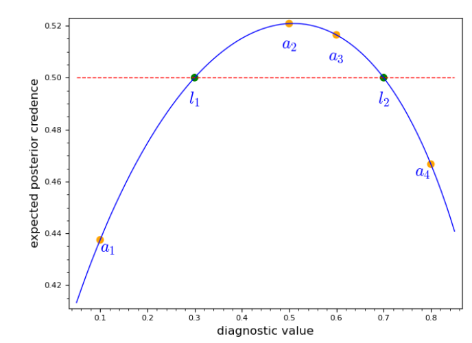
The group of ill-prepared agents can be further subdivided into two groups: those whose diagnostic value is too low (we shall call them low-ill-prepared scientists), and those whose diagnostic value is too high (high-ill-prepared scientist). Formally, $i$ is low-ill-prepared iff $l_1 > P_i(1|H)$ and, $i$ is high-ill-prepared iff $l_2 < P_i(1|H)$. Indeed, the closer an agent’s diagnostic value is to $P(1|H)$, which is the correct value, the more likely she is to successfully evaluate the evidence. An agent only ends up fully supporting $H$ if she updates her beliefs on a substantial number of data points while being well-prepared. In our process of agents influencing each other, agents affect each other’s diagnostic values and thus preparedness for the evidence; therefore, in our model, this process is crucial for the community to reach true consensus.

Results

This section is divided in three parts. First, we elaborate on the way we collect our data. Then, we present an overview of the impact of different parameters, and finally, in the last part we focus on the role of evidence with respect to $\epsilon, \phi$ and $\lambda$.

Stability of the results

As mentioned above, our simulation stops when either 5000 steps have been performed or everybody either supports $H$ or rejects $H$. We observe that the first condition obtains before the second one only in around six runs out of a thousand of them. In those runs, it is always the case that an agent $i$ assigns to $P_i(1|H)$ a value very close to $P_i(1|\neg H)$, and consequently, $i$ would be able to make up her mind about $H$ only if exposed to a very large amount of data. The reason why we impose a 5000 steps limit is that waiting for this to happen would drain computational resources while adding little to none to our results: removing the limit in terms of steps would not change any of our main results.

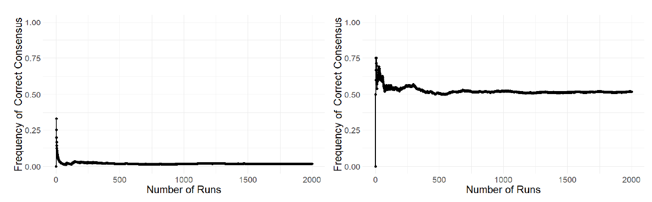
We mainly look at the frequency of an outcome (i.e. correct consensus, wrong consensus, polarization), over 500 runs for a certain parameter combination. In fact, at around 500 runs the value for the frequency becomes stable, as can be seen in Figure 2. In order to provide a reader with the statistical variations of this measure, we include the standard error in the plots we present in the next sections.

**Figure 2.** Frequency of Correct Consensus (y axis) obtained by considering an increasing number of runs (x axis). The first plot considers $\epsilon$ = 0.3, DP = 50, the second $\epsilon$ = 0.5, DP = 10. In every plot, $\lambda$ = 0.5, N = 50, P(1|$\neg$ H) = 0.6.

Reaching consensus

In this section we give an overview of how different factors impact the ability of the community of reaching a correct consensus, i.e.the frequency of correct consensus changes. Before starting, it is worth noting that wrong consensus has a very low frequency ($< 0.05$) in the entire parameter space with the exception of a very small segment that is analysed in the next section. Consequently, whenever the frequency of correct consensus is low, the frequency of polarization is high and vice-versa.

First of all, we observe that the further $P(1|\neg H)$ goes from $0.5$ the more likely the community is to reach correct consensus. Indeed, the larger the distance between $P(1|\neg H)$ and $P(1|H)$, the more likely agents are to start well-prepared and influence other agents to end up fully supporting $H$. Similarly, we observe that increasing the number of agents tends to slightly increase the frequency of a correct consensus: when more agents are initialized the average diagnostic value is more likely to be found close to the real one. As these two patterns are obtained in any other parameter combination we only present results that are obtained with $N = 50$ and $P(1|\neg H) = 0.6$. We choose $N = 50$ and $P(1|\neg H) = 0.6$ as these two values present the community with a fair epistemic challenge, such that reaching a consensus is not too easy, but also not too hard. Every pattern that we highlight in the rest of the results can be observed for almost any other value of $N$ and $P(1|\neg H)$, although its impact may be more or less pronounced. We now turn to analyse the role of $\phi, \epsilon, DP$ and $\lambda$. Figure 3 shows how the frequency of correct consensus changes with respect to the four main parameters.

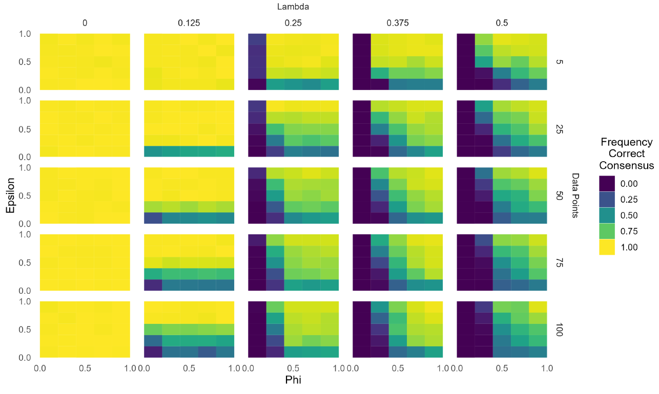
**Figure 3.** The frequency of correct consensus, represented by different colours, with respect to different values of $\phi$, $\epsilon$ and $\lambda$.

Notably, the frequency of correct consensus increases as $\phi$ and $\epsilon$ increase, while it decreases as $\lambda$ decreases, which is in line with our expectations. When $\lambda$ increases, agents are more likely to start with a diagnostic value that is further away from the correct one, i.e. $P(1|H)$. Thus, fewer agents will be well-prepared in inspecting evidence, and more will be prone to reject $H$. By contrast, increasing $\epsilon$ or $\phi$ increases the frequency with which agents influence each other and thereby increases the frequency of correct consensus. This is the result of the following two features of our model.

More discussion leads to more situations in which agents’ diagnostic values are aligned.
Given the design of our model, the correct diagnostic value is never too far from the initial average of diagnostic values of all agents.

As a consequence of these two features, the more agents are able to influence each other’s diagnostic values, the more likely they are to get closer to the correct diagnostic value and become well-prepared. Again, this reflects the idea, well-entrenched among social epistemologists, that discussion and participation are fundamental for scientific communities to be epistemically successful. This result is also in line with any homophily-based bounded confidence model (Flache et al. 2017): the larger the confidence levels of the agents ($\phi$ and $\epsilon$ in our case), the less frequently a community will be polarized.

The impact of evidence

Having established the importance of communication in the model in this way, we turn to another focus point: the impact of evidence and the sample size of batches in which it is gathered. We first explore a section of parameter space which we consider particularly interesting, viz. $\phi \in [0.2, 0.4]$, and then we discuss how the results obtained there generalize for $\phi \in [0,1]$. In general, we present the plots for our results only when $\lambda > 0.2$, as we already indicated that when $\lambda < 0.2$ correct consensus is almost always reached (Figure 3).

More evidence, fewer friends

The interval $\phi \in [0.2, 0.4]$ is particularly interesting since it represents a case in which scientists may be willing to talk with others who have different beliefs about $H$, though they are not able to fruitfully interact with those who hold too different diagnostic values (given their background assumptions or methodological standards).

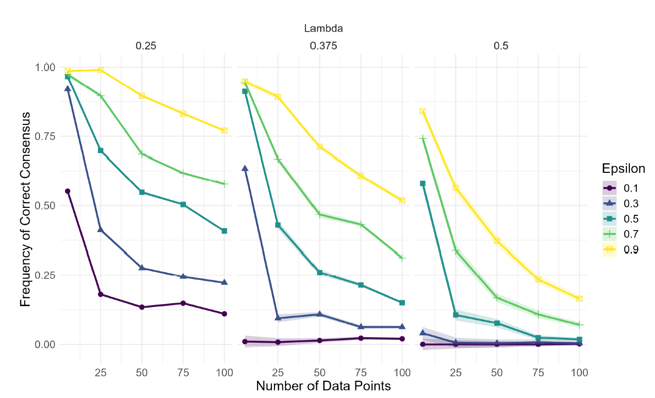
**Figure 4.** The frequency of correct consensus for a community of agents is plotted against the number of data points of every experiment. The colours represent the different values for $\epsilon$, and the subplots the different values for $\lambda$. Notably, $\phi$ = 0.3. The measures for the frequency are obtained over 1000 runs per parameter combination. The small areas around the lines indicate the standard errors over the measures.

In Figure 4 it can be seen that, if the number of data points produced per round increases, the frequency of correct consensus in the community decreases. This result obtains for most values of $\epsilon$, $\lambda$, and $P(1|H)$ if $\phi \in [0.2, 0.4]$. The explanation of this phenomenon is worth considering in some detail. For this, compare two simplified scenarios.

Example 2. Three scientists are ready to investigate a scientific problem: one starts her investigation well-prepared (Section 3.21); let her name be Wilma. The other two have background assumptions that make them ill-prepared for the problem at stake. One of them, Luke, assigns to $P(1|H)$ a lower value than the correct one; the other one, Heidi, assigns a higher value. Now, assume that these scientists individually inspect the outcomes of a big experiment with many data points. Although they interpret the data differently, for each of them this experiment gives ample reason to change their confidence in $H$: Heidi and Luke lower their confidence in $H$ substantially, while Wilma increases hers. The upshot is that later, when meeting at a conference, they do not talk with each other: Wilma is too confident in $H$ to discuss with people who take $\neg H$ to be more likely, and Heidi and Luke, although they think similarly of $H$, do not speak because of their difference in background assumptions. Consequently, none of them changes their diagnostic values, leaving Luke and Heidi equally ill-prepared for the next round of experimental data. After a number of such rounds, Wilma will fully support $H$ while Heidi and Luke will fully reject it. Hence, they will end up polarized.

Example 3. In the same setting, the three scientists are exposed to fewer data points. Now, Luke and Heidi lower their confidence in $H$ only slightly, whereas Wilma increases hers slightly. Then, when they meet at the conference, the difference in background assumptions still prevents Luke and Heidi from interacting, but Wilma interacts with both. As a result, Luke increases his diagnostic value, while Heidi decreases hers. This leaves Luke and Heidi minimally less ill-prepared for the next round of experimental data, since their diagnostic values will be closer to the correct one (Section 3.21); potentially, all three will be well-prepared. In the new round of data, the process is repeated, increasing the chance that Luke and Heidi become well-prepared: once all three of them agree on the (correct) diagnostic value, they are guaranteed to end up supporting $H$.

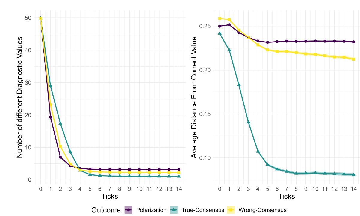
In short, exposure to fewer data points prevents scientists from radicalizing their positions in terms of $H$, and consequently, increases the likelihood of a fruitful interaction that leads them to correcting their diagnostic values. In fact, if a consensus will be reached, the agents’ diagnostic values start to get relevantly closer to the correct one already in the third step (Figure 5, on the right). Conversely, in runs that do not result in the community reaching the correct consensus, the average distance from the correct diagnostic value remains large, and stabilizes at some point: here, ill-prepared agents only interact with other ill-prepared agents, and thus never correct their diagnostic values. Still, even in those cases, agents continue to influence and be influenced by other agents: the number of unique diagnostic values decreases regardless of the final outcome (Figure 5, on the left).

**Figure 5.** On the left the average number of unique diagnostic values is plotted against the passing of time (ticks). On the right the average distance from the correct value P(1|H) of each agent’s diagnostic value is plotted against the passing of time (ticks). In both cases, the mean is obtained by grouping the runs with respect to their final outcome: polarization, correct consensus and wrong consensus. The measures are obtained with by running our model 10000 times with $\lambda$ = 0.5, $\phi$ = 0.3, $\epsilon$ randomly drawn from the uniform distribution between 0 and 1, and DP randomly drawn between 5 and 100, and then dividing each run based on the final outcome.

In addition, note that in Figure 4, the largest difference is between 5 and 25 data points. This is a consequence of Bayesian updating: the difference between the prior and the posterior belief (that is, $|P_i^t(H)-P_i^{t+1}(H)|$) increases drastically when going from 5 to 25 data points, and hardly at all when going from 75 to 100 data points.

So far, we observed that access to less evidence tends to facilitate correct consensus, and we explained why: with fewer data points, agents are less likely to radicalize their positions such that it disrupts their communication with scientists who are well-prepared for the evidence. Yet, reducing the number of data points has negative side effects. These are represented in Figure 6 and Figure 7.

**Figure 6.** The frequency of a wrong consensus for a community of agents is plotted against the number of data points of every experiment. The colours represent the different values for $\epsilon$, and the subplots the different values for $\lambda$. Notably, $\phi$ = 0.3. The measures for the frequency are obtained over 1000 runs per parameter combination. The small areas around the lines indicate the standard errors over the measures.

**Figure 7.** The average time for a run is plotted against the number of data points of every experiment. The colours represent the different values for $\epsilon$, the subplots the different values for $\lambda$. We let $\phi$ = 0.3. The measures for the frequency are obtained over 1000 runs per parameter combination. The small areas around the lines indicate the standard errors over the measures.

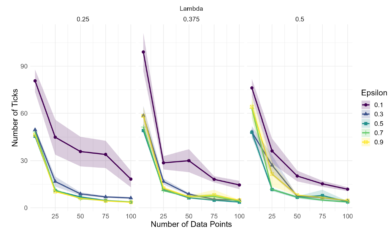
Having fewer data points may, in certain cases, increase the amount of time needed to reach consensus as well as the frequency of wrong consensus. The first feature is easily explained: even well-prepared agents need a certain number of data points to move their confidence in $H$ towards full rejection or full support. With fewer data points at each step, more steps are needed.

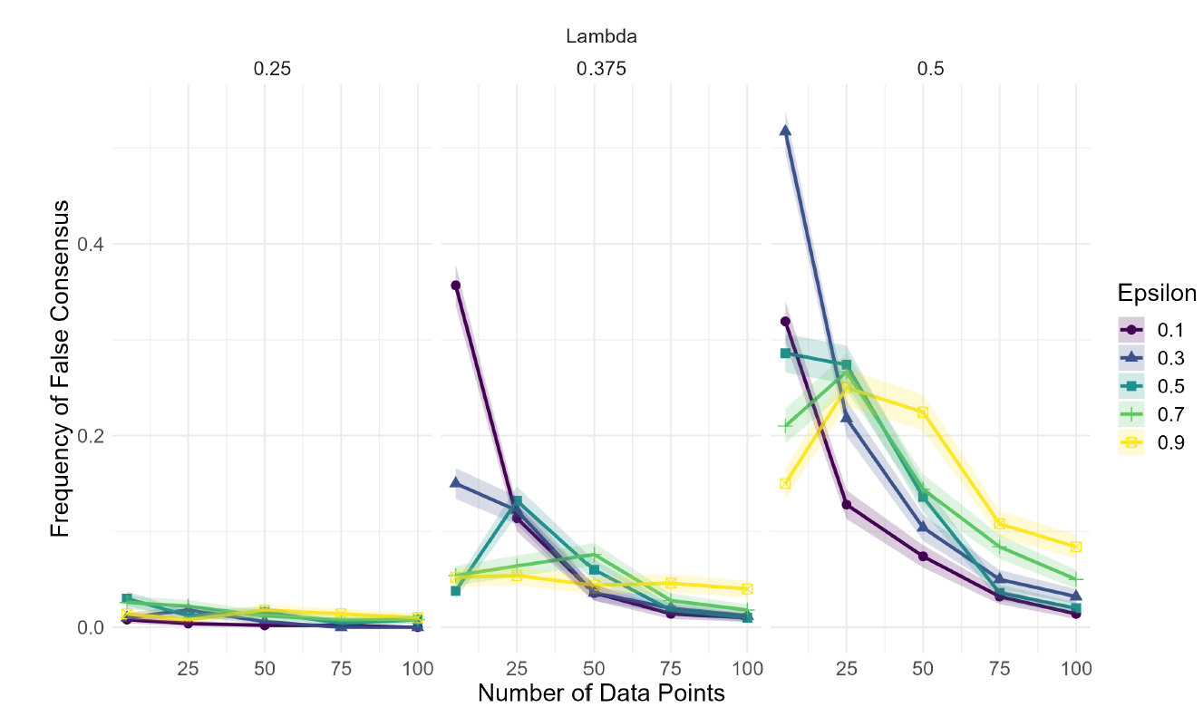
The emergence of wrong consensus is more interesting, as it is also specific of these parameter combinations. In general, similarly to correct consensus, wrong consensus becomes more frequent, because with less data points agents tend to discuss more and consequently they tend to converge more on the same diagnostic values. Yet, why does the community mostly converge on correct consensus and only sometimes on a wrong one? In Section 3.21 we mentioned that agents can be divided into three groups, based on their diagnostic values: the well-prepared, the low-ill-prepared and the high-ill-prepared. In correct-consensus runs, interactions between scientists from different groups lead to the formation of a new larger group, which consists of only well-prepared agents. This is because the scientists that were well-prepared already in the beginning interact equally with both other groups, and possibly also the other groups interact with each other, converging on the average diagnostic value (which is also the correct one). Conversely, in wrong-consensus runs, it is most likely that the group of well-prepared agents interacts with only one group of ill-prepared agents, e.g.a piece of evidence has pushed these two groups closer to one another in terms of beliefs. As a result, the group of well-prepared agents is absorbed by one of the ill-prepared ones, fostering the division in two groups: both ill-prepared. In fact, runs that end in a wrong consensus typically feature a division of agents into two groups with respect to their diagnostic values (Figure 5). This is a marked difference from correct-consensus runs, which typically feature only one group. Such a mechanism explains why the frequency of wrong consensus increases only when $\lambda$ is quite high and $\epsilon$ is quite low. On the one hand, when $\epsilon$ is low, it is more likely for well-prepared scientists to interact only with members of one group of ill-prepared ones, whereas the more $\epsilon$ increases, the more likely agents are to include in their group of influencers scientists from both sides. On the other hand, the higher $\lambda$ the larger are the groups of ill-prepared agents, which makes it easier for them to move the well-prepared ones away from their diagnostic values.

For a better understanding of the role evidence plays in the model, it is worth examining the frequency of wrong consensus with respect to the data points that are available to the agents. Indeed, the results indicate that decreasing the number of data points may also have a harmful effect by increasing the chances of getting a wrong consensus. However, note that neither the spread nor the strength of this correlation (between number of data points and the wrong consensus) is comparable to those of the correlation between number of data points and correct consensus. The latter obtains for almost any parameter value (given that $\phi \in [0.2, 0.4]$) and may drastically diminish the chances of a correct consensus (e.g.the case of $\epsilon = 0.3$ and $\lambda = 0.375$ of Figure 4), whereas the former only obtains for low values of $\epsilon$ and high ones of $\lambda$, and often generates marginal effects (increasing the number of data points never decreases the frequency of wrong consensus by more than 0.5).

More evidence, same friends: Broadening the parameter space

In the previous section, we highlighted the results obtained for $\lambda = 0.3$. Those results indicate that increasing the number of data points decreases the frequency of a correct consensus, i.e. they are negatively correlated. However, this negative correlation does not generalize. Consider Figure 8: given that $\lambda$ is not too low, a strong correlation between the two is present only when $\phi \in [0.2, 0.4]$.

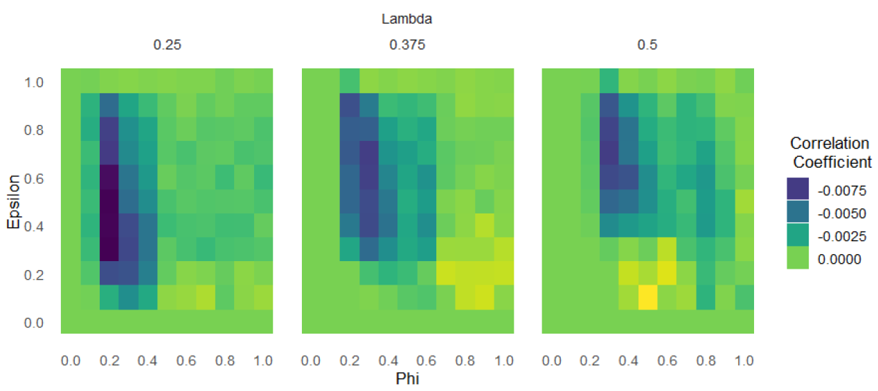
**Figure 8.** The correlation between the number of data points and the frequency of correct consensus is represented by the colors of the tiles. The plot covers any possible parameter combination such that i.e. $\lambda \in$ [0.1, 0.5], $\phi \in$ [0,1], $\epsilon \in$ [0,1].

The reason is the following. If the number of data points is low enough (indicatively lower than 20), the mechanism described in paragraph 1.1.4 1 obtains: the agents remain close enough in terms of beliefs, and by doing so they manage to discuss and converge on a value that is close enough to the correct diagnostic value. If the number of data points is high, initially nothing changes with respect to the mechanism we already described: both groups of ill-prepared agents substantially revise their beliefs in the direction of supporting $\neg H$, and the group of well-prepared ones moves towards $H$. However, if $\phi$ is low, agents coming from the (low)ill-prepared group and the (high)ill-prepared group do not talk, while if $\phi$ is high, they can influence each other. This leaves them arriving at the average of their diagnostic values, which happens to be closer to the correct value. We consider this result as an extreme consequence of our assumption of a ‘wisdom of the crowd.’⁶

In addition, other patterns can be noted in Figure 8. When $\phi$ or $\epsilon$ is very low, the number of data points has hardly any effects, since agents fail to interact or only interact with scientists whose diagnostic values are already close to theirs. Similarly, when $\epsilon$ is very high, it is highly likely that agents will influence each other early on in the simulation regardless of the amount of evidence, and consequently, the number of gathered data points won’t have a significant impact. For very similar reasons, a correlation between wrong consensus and number of data points is never present for $\phi$ outside of the interval $[0.2, 0.4]$.

Sensitivity analysis

We performed a variance-based global sensitivity analysis in order to reveal the complex ways in which input factors influence the model outcome.⁷ Since we are exploring the relationship between disagreement over the diagnostic value of evidence and the epistemic performance of a community of scientists, the main output of interest is the frequency of correct consensus within the community. The results of the model are conditional on several factors, out of which six are selected as input parameters with a discrete uniform distribution. Table 3 summarizes the selection of the model parameters and the value range for each of them. A single computational experiment (4.860.000 simulations) with a full factorial design was carried out.

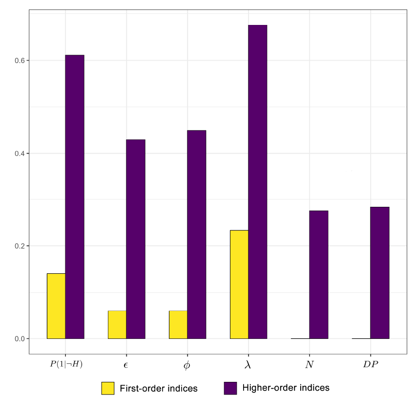
**Figure 9.** Variance decomposition of effects on model result (frequency of correct consensus within the scientific community). Two measures are depicted: first-order indices (S) and higher-order indices (ST).

It is worth mentioning that the average value for the frequency of correct consensus is 0.78 (SD = 0.4) over all paramaters values. The results of the experiment are shown in Figure 9. The highest first-order index is $\lambda$ (23% of total variance), followed by $P(1|\neg H)$ (14%). Factors $N$ and $DP$ have the lowest value, meaning that their contribution to the variability of the output is minimal when considered in isolation. Therefore, the generation of a correct consensus within a scientific community is predominantly driven by the initial dispersion of agents’ background assumptions. In sum, all first-order indices amount to only 35% of the frequency of correct consensus variability, which is the percentage of the output variance that can be explained by examining the factors individually. The remaining 65% of variability is to be attributed to complex factor interrelation. Every factor significantly contributes to the model’s complex behavior, as higher-order indices show. This suggests that the frequency of correct consensus within a scientific community is a matter of a complex, interrelated set of factors.

Discussion

In this section we compare our results with some related findings and discuss their more general implications.

As mentioned above, our approach to modeling epistemic communities is similar to network epistemology bandit models, such as those by Zollman (2007, 2010). A well-known finding from these models is the so-called Zollman effect, according to which a high degree of information flow in a scientific community may impede the formation of a correct consensus. Since our results also highlight factors that may impede the formation of a correct consensus in communities that fully share evidence, one may wonder how they relate to Zollman’s findings.

On the one hand, in Zollman’s model, scientists do not disagree on the diagnostic value of evidence and increasing the sample size of experiments is strictly beneficial (Rosenstock et al. 2017). Our model qualifies these insights. We show that if scientists disagree on the diagnosticity of evidence, larger amounts of data points produced by experiments may lead to lower correct consensus rates. On the other hand, our results are consistent with the Zollman effect in the sense that the underlying mechanism leading the community away from the correct consensus is an initial spread of misleading information. In Zollman’s model this is caused by dense social networks, while in our model by agents misinterpreting large amounts of evidence.

The fact that in our model larger sample sizes lead to less successful inquiry in case agents disagree on how they interpret data, does not imply that scientists should conduct studies of a smaller sample size. Indeed, there are very good reasons, independent of those discussed in this paper, why large-scale studies are beneficial. Rather, our results suggest that, given that large-scale studies are typically beneficial, one might have to take additional measures to preempt problematic scenarios illustrated above.⁸ For instance, such a precautionary measure could include taking into account the presence of a peer-disagreement as a ‘higher-order evidence’ which lowers one’s confidence in one’s current belief on the matter (Friedman & Šešelja 2022; Henderson 2022). Moreover, the scientific community could introduce measures encouraging discussion among disagreeing scientists on the diagnosticity of the evidence (for example, by organizing conferences targeting such issues).

Indeed, our results also highlight that reducing the sample size may not always have positive effects. As a lower number of data points increases the cohesiveness of the community, it may also increase the chances of a wrong consensus. Although the conditions for this to happen are very specific, such a finding exemplifies the duality of a cohesive community. In most of the cases, a cohesive community is effective: scientists together increase their confidence in the correct answer. Yet, if such cohesion is obtained around the wrong way of interpreting evidence, all scientists may end up supporting the worse hypothesis.

It is worth noting that this model carries some limitations. First, it is reasonable to assume that in scientific practice, at least some disagreements arise from the fact that scientists don’t use the same methods. For instance, in the model developed by Douven (2019), some agents use Bayes’ rule to update while others use probabilistic versions of inference to the best explanation that change their degrees of belief. In our model, we take all agents to be Bayesian updaters. While it is true that other methods of belief updating would be worth exploring, for our initial model we decided to use the standardized Bayesian updating approach. Second, an ideal scenario would involve the simulation and the analysis of random choices for $P(1|H)$ and $P(1|\neg H)$ (in the model we assume that $P(1|\neg H) \in [0.55, 1)$, see Section ). This is not addressed in the present paper because of computational tractability reasons. If the value of $P(1|\neg H)$ is too close to $P(1| H)$, agents need very large amounts of evidence to either support or reject $H$, which requires simulations to run for a very long time. The implementation in NetLogo and consequent slow execution makes our model unsuitable for studying this ideal scenario.

Conclusion

In this paper we introduced an ABM for studying scientific polarization in a community whose members may diverge in the way they interpret the available evidence. Agents in the model represent scientists who are trying to decide whether a certain hypothesis $H$ is true. To this end, they perform Bayesian belief updates after receiving experimental results. Since they consider evidence to different degrees diagnostic of $H$, their belief updates may also diverge, even if based on the same experiments. Moreover, through discussions on their background assumptions, they can influence each other and either converge on a common diagnostic value for the evidence, or remain divided on this issue. Our results indicate that, in general, the more willing the agents are to discuss their background assumptions, the more likely the community is to reach a correct consensus. This is in line with the results that have usually been obtained in opinion dynamics models based on a homophily type of influence (Flache et al. 2017). Furthermore, our results also suggest that increasing the sample size of experiments may be detrimental to the community, since for certain parameter combinations, it drastically decreases the chances of achieving a correct consensus. Yet, at the same time, decreasing the sample size of experiments may not always be beneficial: under specific parameters a decrease in sample size can make a wrong consensus more likely. In light of these features, our model fills a gap in the literature on scientific polarization since it shows how polarization can emerge even if agents fully share evidence and don’t discount any of the gathered data, but treat all evidence as equally certain.

Since the current model is exploratory, it leaves room for further enhancements and variations. For instance, it would be interesting to examine the robustness of our results once the ‘wisdom of the crowd’ assumption is relaxed so that agents do not start with diagnostic values, the average of which is close to the correct one. Moreover, examining potential mitigating mechanisms (such as measures mentioned in the previous Section) would be a way of investigating the question: how can we improve the performance of a community whose members disagree on the diagnosticity of the evidence?

Acknowledgments

We would like to thank the anonymous referees of this paper, the participants of the Social Simulation (SSC) Conference (12-16 September 2022 | University of Milan, Italy), the participants of the European Network for the Philosophy of the Social Sciences (ENPOSS) Congress (21-23 September 2022 | University of Málaga, Spain) and Soong Yoo for their comments and suggestions. This research was supported by the Ministerio de Economía y Competitividad (grant number FFI2017-87395-P) and by the Deutsche Forschungsgemeinschaft (DFG, German Research Foundation) – project number 426833574.

Appendix A: Mathematical Analysis

In this section, we briefly explain how the division in well-prepared and ill-prepared agents is obtained. An agent $i$ is well-prepared in case its expected posterior value for $H$ is greater than $.5$. The expected posterior value in $H$ for $i$ at time point $t$ is computed by a function $\mathsf{exp}:[0,1] \mapsto [0,1]$, which takes as an input the diagnostic value $P_i^t(1|H)$ of agent $i$. In particular, for a given diagnostic value $x$ and for a single draw from the probability distribution $P(| H)$ the expected posterior value is obtained as follows: \[\begin{multline*} \mathsf{exp}(x) = P(1|H) \cdot \underbrace{P_i^t(H) \cdot x \cdot \frac{1}{P_i^t(H) \cdot x + P_i^t(\neg H) \cdot P(1 | \neg H)}}_{P_i^{t+1}(H|1)} + \\ P(0 | H) \cdot \underbrace{P_i^t(H) \cdot (1-x) \cdot \frac{1}{P_i^t(H) \cdot (1-x) + P_i^{t}(\neg H) \cdot (1 - P(1| \neg H))}}_{P_i^{t+1}(H|0)}. \end{multline*}\] Assuming a prior $P_i^t(1 | H)$ of $.5$, the equation $\mathsf{exp}(x) = .5$ has two solutions, $l_1 = 1- P(1 | H) \,\text{and}\, l_2 = P(1 | H)$. In other words, an agent whose diagnostic value $P_i^t(1 | H)$ is strictly in the interval $(l_1, l_2)$ has an expected posterior credence in $H$ of greater than $.5$, otherwise at most $.5$. The same applies to experiments of sample sizes greater than 1, since such experiments can be equivalently modeled by iterative single draws. We also note that all agents start the simulation with a prior of $.5$ and whenever the diagnostic value is updated (as a result of a social exchange), all previous experimental results get reevaluated with a prior of $.5$. It is therefore sufficient to determine the solution of $\mathsf{exp}(x)$ with a prior of $.5$.

Appendix B: ODD Protocol

This section presents the model according to Grimm et al. (2020) ODD protocol. As a consequence, the terms and notions we employ here to describe our model are intended in the way Grimm et al. (2020) define them.

References

DEFFUANT, G., Amblard, F., Weisbuch, G., & Faure, T. (2002). How can extremism prevail? A study based on the relative agreement interaction model. Journal of Artificial Societies and Social Simulation, 5(4), 1. [doi:10.18564/jasss.2211]
DE Langhe, R. (2013). Peer disagreement under multiple epistemic systems. Synthese, 190, 2547–2556. [doi:10.1007/s11229-012-0149-0]
DOUVEN, I. (2010). Simulating peer disagreements. Studies in History and Philosophy of Science Part A, 41(2), 148–157. [doi:10.1016/j.shpsa.2010.03.010]
DOUVEN, I. (2019). Optimizing group learning: An evolutionary computing approach. Artificial Intelligence, 275, 235–251. [doi:10.1016/j.artint.2019.06.002]
DOUVEN, I., & Hegselmann, R. (2022). Network effects in a bounded confidence model. Studies in History and Philosophy of Science, 94, 56–71. [doi:10.1016/j.shpsa.2022.05.002]
FLACHE, A., Mäs, M., Feliciani, T., Chattoe-Brown, E., Deffuant, G., Huet, S., & Lorenz, J. (2017). Models of social influence: Towards the next frontiers. Journal of Artificial Societies and Social Simulation, 20(4), 2. [doi:10.18564/jasss.3521]
FRIEDMAN, D. C., & Šešelja, D. (2022). Scientific disagreements, fast science and higher-order evidence. Forthcoming. Available at: http://philsci-archive.pitt.edu/21246/ [doi:10.1017/psa.2023.83]
GRIMM, V., Railsback, S. F., Vincenot, C. E., Berger, U., Gallagher, C., DeAngelis, D. L., Edmonds, B., Ge, J., Giske, J., Groeneveld, J., Johnston, A. S. A., Milles, A., Nabe-Nielsen, J., Polhill, J. G., Radchuk, V., Rohwäder, M. S., Stillman, R. A., Thiele, J. C., & Ayllón, D. (2020). The ODD protocol for describing agent-Based and other simulation models: A second update to improve clarity, replication, and structural realism. Journal of Artificial Societies and Social Simulation, 23(2), 7. [doi:10.18564/jasss.4259]
HAHN, U., & Hornikx, J. (2016). A normative framework for argument quality: Argumentation schemes with a Bayesian foundation. Synthese, 193(6), 1833–1873. [doi:10.1007/s11229-015-0815-0]
HEGSELMANN, R., & Krause, U. (2002). Opinion dynamics and bounded confidence models, analysis, and simulation. Journal of Artificial Societies and Social Simulation, 5(3), 2.
HEGSELMANN, R., & Krause, U. (2006). Truth and cognitive division of labor: First steps towards a computer aided social epistemology. Journal of Artificial Societies and Social Simulation, 9(3), 10.
HENDERSON, L. (2022). Higher-Order evidence and losing one’s conviction. Noûs, 56(3), 513–529. [doi:10.1111/nous.12367]
KOPECKY, F. (2022). Arguments as drivers of issue polarisation in debates among artificial agents. Journal of Artificial Societies and Social Simulation, 25(1), 4. [doi:10.18564/jasss.4767]
LIGMANN-ZIELINSKA, A., Siebers, P.-O., Magliocca, N. R., Parker, D. C., Grimm, V., Du, J., Cenek, M., Radchuk, V., Arbab, N. N., Li, S., Berger, U., Paudel, R., Robinson, D. T., Jankowski, P., An, L., & Ye, X. (2020). One size does not fit all: A roadmap of purpose-driven mixed-method pathways for sensitivity analysis of agent-based models. Journal of Artificial Societies and Social Simulation, 23(1), 6. https://doi.org/10.18564/jasss.4201 [doi:10.18564/jasss.4201]
LONGINO, H. (2002). The Fate of Knowledge. Princeton, NJ: Princeton University Press.
LONGINO, H. E. (2022). What’s social about social epistemology? The Journal of Philosophy, 119(4), 169–195. [doi:10.5840/jphil2022119413]
MÄS, M., & Flache, A. (2013). Differentiation without distancing. Explaining bi-polarization of opinions without negative influence. PLoS One, 8(11), e74516.
MOREY, R. D., Romeijn, J.-W., & Rouder, J. N. (2016). The philosophy of Bayes factors and the quantification of statistical evidence. Journal of Mathematical Psychology, 72, 6–18. [doi:10.1016/j.jmp.2015.11.001]
O’CONNOR, C., & Weatherall, J. O. (2018). Scientific polarization. European Journal for Philosophy of Science, 8(3), 855–875.
OLSSON, E. J. (2013). A Bayesian simulation model of group deliberation and polarization. In F. Zenker (Ed.), Bayesian Argumentation (pp. 113–133). Berlin Heidelberg: Springer. [doi:10.1007/978-94-007-5357-0_6]
PALLAVICINI, J., Hallsson, B., & Kappel, K. (2018). Polarization in groups of Bayesian agents. Synthese, 198(1), 1–55. [doi:10.1007/s11229-018-01978-w]
ROSENSTOCK, S., Bruner, J., & O’Connor, C. (2017). In epistemic networks, is less really more? Philosophy of Science, 84(2), 234–252. [doi:10.1086/690717]
SINGER, D. J., Bramson, A., Grim, P., Holman, B., Jung, J., Kovaka, K., Ranginani, A., & Berger, W. J. (2017). Rational social and political polarization. Philosophical Studies, 176, 1–25. [doi:10.1007/s11098-018-1124-5]
STEGENGA, J. (2016). Three criteria for consensus conferences. Foundations of Science, 21(1), 35–49. [doi:10.1007/s10699-014-9374-y]
ZOLLMAN, K. J. (2007). The communication structure of epistemic communities. Philosophy of Science, 74(5), 574–587. [doi:10.1086/525605]
ZOLLMAN, K. J. (2010). The epistemic benefit of transient diversity. Erkenntnis, 72(1), 17–35. [doi:10.1007/s10670-009-9194-6]