An Assimilation Anomaly: Averaging-Induced Reversal of Overall Opinion in Two Interacting Societies

and
aDepartment of Atmospheric Science, Colorado State University, United States; bW. M. Keck Science Department of Claremont McKenna College, Pitzer College, and Scripps College, United States
Journal of Artificial
Societies and Social Simulation 26 (4) 6
<https://www.jasss.org/26/4/6.html>
DOI: 10.18564/jasss.5150
Received: 23-Nov-2022 Accepted: 08-Jul-2023 Published: 31-Oct-2023
Abstract
Assimilation – the tendency for individuals to adjust their opinions to more closely align with those around them – is one of the central components of computational social-influence and opinion-dynamics models that seek to elucidate how large-scale societal trends can emerge from local social interactions among small groups of individuals. Although assimilation processes have been well studied using increasingly sophisticated assimilative schemes like bounded confidence, nonlinear opinion-averaging methodologies, time-varying social network structures, etc., we show there is a surprising, previously unrecognized phenomenon lurking in even the simplest of assimilation models. We consider here two societies that start out on opposite sides of some opinion spectrum, for instance, one initially very conservative society and the other very liberal. We assume small groups of individuals from these societies can meet and interact, and that during an interaction each person’s opinion simply moves closer to the average opinion of the group. One might anticipate that this barebones assimilation process – which involves nothing more than simple numerical averaging of opinions during each encounter – will invariably lead to a steady (and rather uninteresting) convergence of overall opinion among the two societies wherein the initial intersocietal differences are straightforwardly washed away. We show instead that a counterintuitive, large-scale demographic reversal can sometimes emerge – i.e., the two societies can potentially end up swapping their relative positions on the opinion spectrum, with the initially conservative society ending up more liberal, on the whole, than the formerly liberal society. This finding (dubbed an “assimilation anomaly”) shows how the process of repeatedly taking simple averages on a local level can induce an overall reversal of average opinion on a global level. Using a heat diffusion model from physics, we reveal the origins of this curious phenomenon. This dynamical effect involving two interacting societies is wholly distinct from other interesting social-influence phenomena described in the opinion-dynamics literature (e.g., polarization, fragmentation, phase transitions, bifurcations, etc.).Introduction
In an effort to better understand the structure and dynamics of societies, computational social scientists often employ multi-agent models governed by relatively simple interaction rules to simulate the behaviors of large systems with many interacting components. Such models have proven to be highly informative and serve as useful complements to traditional approaches based on large-scale empirical data. A particularly prominent class of social-influence models, known as opinion-dynamics models, focus on how beliefs and opinions in a society evolve and their underlying mechanisms of transmission. In broadest terms, social-influence or opinion-dynamics models assume individual agents possess some set of socially malleable traits (i.e., opinions or beliefs) that can be influenced by social interactions with other agents and explore the dynamical evolution of these beliefs across society as these interactions progress. Opinion-dynamics models are quite versatile, with direct applications across many disciplines including political science, sociology, and economics, as evidenced by a vast and burgeoning literature (e.g., Xia et al. 2011; Axelrod 1997; Castellano et al. 2000, 2009; Currin et al. 2022; Hegselmann & Krause 2002; Keijzer & Mäs 2022; Kuperman 2006; Lorenz 2007; Nguyen et al. 2021; Peralta et al. 2023; Sirbu et al. 2016; Vespignani 2011; Weisbuch et al. 2002). Indeed, numerous strains of opinion-dynamics models have been developed, being differentiated from one another based on whether the model’s opinion state variable is continuous, discrete, a scalar or a vector (e.g., Hegselmann & Krause 2002); the choice of averaging algorithm that governs the weighting of opinions during the multi-agent interactions (e.g., Krause 2000; Friedkin & Johnsen 2011; Hegselmann & Krause 2002; Kuperman 2006); the restrictions or constraints on the sets of agents who can participate in the opinion-averaging process (e.g., in bounded confidence models only agents whose opinions are sufficiently similar can interact; in Axelrod’s cultural assimilation model the assumption of homophily bases the likelihood of interactions between two agents on how similar the agents are to one another and does not permit two agents who are completely dissimilar to interact) (e.g., Axelrod 1997; Dittmer 2001; Hegselmann & Krause 2002); whether there is an underlying social network/graph structure in the model and whether any such underlying network is static or evolves in time (e.g., Fennell et al. 2021; Pfau et al. 2013; Reia & Fontanari 2016; Stivala & Keeler 2016; Vazquez et al. 2007); the communication scheme used by the agents (e.g., one-to-one, one-to-many, many-to-one) (Abelson 1964; Flache & Macy 2011; Friedkin & Johnsen 2011; Keijzer et al. 2018; Shibanai et al. 2001); whether a mass media influence is present or not (e.g., Daley & Kendall 1964; Peres & Fontanari 2012; Pineda et al. 2009; Rodríguez et al. 2009); the inclusion or omission of noise (e.g., Gandica et al. 2013; Flache & Macy 2011; Klemm et al. 2003; Parisi et al. 2003); etc.
Despite this tremendous variety of model types and assumptions, assimilation represents a common, unifying theme underlying the vast majority of these social-influence or opinion-dynamics models, i.e., virtually all these models include some type of assimilative mechanism by which interacting agents adjust their views in light of the opinions of others, with the general tendency being for interacting agents to become more similar during any given encounter. Typically, in an assimilative interaction involving multiple agents, the agents will neither completely adopt nor completely disregard the opinions of the other participating agents, but instead will take a partial step towards their collective middle ground, which is usually computed by taking some sort of weighted average of opinions of the agents (see, e.g., Friedkin & Johnsen 2011). Often assimilation proceeds in a very straightforward manner, particularly if few restrictions or limitations are placed on the opinion-averaging process itself. For instance, in very simple assimilation scenarios involving a single society, the process of repeatedly averaging over the opinions of various groups of agents in that society will eventually wash away differences and ultimately produce consensus throughout the society (i.e., complete uniformity in the opinions of the agents), also known as a mono-culture in some contexts. In more sophisticated assimilation models where various constraints, restrictions, or other stipulations are placed on the assimilative averaging mechanism (e.g., as in bounded-confidence models where agents that are very different from one another cannot interact, or in models where agents’ opinions harden over time, etc.), complete assimilation within the society may never reach fruition and other interesting behaviors can result, such as the polarization or fragmentation of opinions, or the appearance of phase transitions (e.g., Castellano et al. 2000).
In this paper we illustrate a novel, seemingly anomalous effect that can arise even in the simplest of assimilation models where one would normally not expect any surprises. First consider a single society in which small groups of agents are interacting, and during those interactions the agents’ opinion values each just move closer toward their common numerical group average (without any complicating factors like bounded confidence restrictions, time-varying weights in the averaging process, etc.). (See Section 2 for details.) In this simplistic scenario, the process of repeatedly numerically averaging the opinions of different agents will ultimately produce a state of complete consensus within a society, as expected. The surprise happens when we instead consider two such societies, this time assuming that assimilation is not only occurring within each society but now also allow for inter-societal assimilation wherein agents from one society can briefly visit, interact, and assimilate with agents in the other society before returning home. We assume the same simplistic numerical opinion-averaging mechanism is at work for both these inter-societal and intra-societal interactions. What we discover is that this seemingly straightforward assimilation mechanism – even though it is based entirely on simple numerical averaging of opinions – can yield a nontrivial result among the two interacting societies, namely, reversals in the overall opinion characteristics of the two societies during the course of their interactions. For instance, consider two societies where the agents’ opinion values can lie anywhere between 0 and 100 on some (continuous) numerical opinion spectrum. Agents are free to interact with neighboring agents in their own society, and/or can briefly visit and interact with an agent and its neighbors in the other society. During each encounter we assume the basic group opinion-averaging process described above is carried out. Now suppose the two societies start out extremely polarized, where initially every agent in one society has an opinion value of 100, while every agent in the second society has an initial opinion value of 0. As small groups of agents repeatedly interact and assimilate with one another (both within their own society and when visiting the other society), an unexpected phenomenon can emerge: at some point in their evolution, it is possible that the average opinion in the first society could drop below that of the second society (e.g., the first could drop from 100 to, say, 40, while the average opinion in the second society could rise from 0 to a value of 60). This unexpected reversal in overall societal opinions typically appears as a transient, intermediate state of the system, and if the assimilation process is allowed to proceed indefinitely eventually a state of complete uniformity within and between the two societies will ultimately result (though under certain choices of the model’s parameters this reversal can sometimes persist). Regardless, the existence of a potential reversal of the two societies’ relative positions on the opinion spectrum under this humblest of assimilation mechanisms (based on nothing more than simple numerical averaging) is in many respects quite surprising, and is the main focus of this paper.
The goal of this work is a modest one. With the help of a very elementary opinion-dynamics model, we illustrate and analyze this rather curious, previously unrecognized facet of assimilation. We do not attempt to directly match our numerical findings to specific real-world empirical data drawn from any particular case study, but instead wish to highlight here the existence of this surprising dynamical phenomenon which can lurk in even very simple social-influence/opinion-dynamics models. The paper is structured as follows: in Section 2 we introduce a very basic, stripped-down multi-agent model describing assimilation in two societies (intentionally devoid of bells and whistles so as to cleanly exhibit the effect); Section 3 documents our numerical findings and observations of the “assimilation anomaly,” and describes various associated dynamical trends seen in our simulations. In Section 4 we lay out the intuitive, conceptual, and theoretical underpinnings that explain how and why an assimilation anomaly can arise, focusing on an analogous heat diffusion model from physics. Section 5 summarizes our findings and discusses extensions.
The Basic Assimilation Model
Below we outline the basic opinion-dynamics model that we will use to illustrate the emergence of the assimilation anomaly. We emphasize from the outset that many of the particular choices we make for the model are largely for purposes of convenience and simplicity of illustration, and that the assimilation anomaly described in this paper is a fairly robust phenomenon that can emerge even if a number of the model’s specific features are altered. For instance, in our model we will assume nearest-neighbor interactions on a simple grid-like network. However, the effect can still emerge even if we drop the simple grid-like structure and instead assume that an agent visiting the other society can simultaneously interact with all agents in that society, not merely nearest neighbors; this drastic change in underlying network structure does not suppress the emergence of the assimilation anomaly and in fact can even sometimes enhance it. Similarly, though we will impose doubly period boundary conditions to eliminate edge effects on the square lattices representing the two societies, this choice of boundary conditions is done for convenience and has little bearing on the overall outcome.
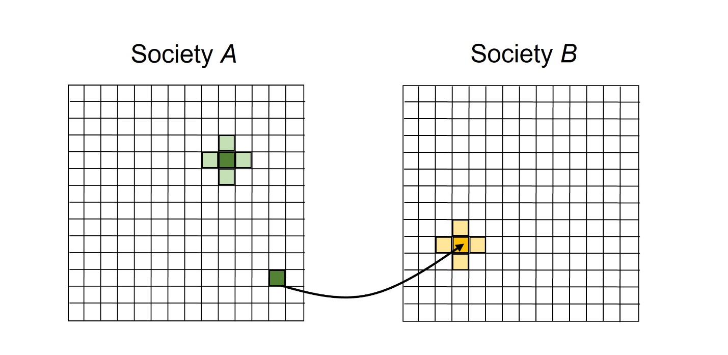
We begin by considering two societies, \(A\) and \(B\), composed of agents located on square lattices of sizes \(N_{A} \times N_{A}\) and \(N_{B} \times N_{B}\), respectively, as shown in Figure 1. Individual agents in each society are denoted respectively by \(A_{ij}\) and \(B_{ij}\), where the indices \(i,j\) of \(A_{ij}\) run from \(1,2, \dots, N_{A}\) while those of \(B_{ij}\) run from \(1,2, \dots, N_{B}\). When we don’t wish to explicitly specify which society an agent resides in, we will use \(X_{ij}\) to denote a generic agent (while keeping in mind that the upper limits for the indices \(i,j\) will depend on which of the two societies the agent actually resides in). Each agent is assumed to hold a (scalar, real-valued) opinion whose numerical value lies in the range [0,100] (this choice of a 100-point range for the opinion scale is arbitrary and has no bearing on the model’s behavior.) As it should not cause any confusion based on context, we will use \(X_{ij}\) both to denote the agent located at lattice point \(i,j\) as well as to denote the numerical value of that agent’s opinion. Every agent \(X_{ij}\) is assumed to have four nearest neighbors, namely \(X_{i,j-1}\), \(X_{i,j+1}\), \(X_{i-1,j}\), \(X_{i+1,j}\), where for convenience we assume doubly periodic (toroidal) boundary conditions on the lattices.
Assimilation proceeds in a straightforward, iterative fashion, as follows: At each step, a small group of agents is selected (as described below) and the opinion of each member of this group is moved closer to the average opinion of the group, denoted \(\overline{X}\). More precisely, letting \(X_{ij}\) denote the opinion value of an agent in the selected group, the agent’s updated opinion value is:
| \[ X_{ij} \rightarrow X_{ij} + s(\overline{X} - X_{ij})\] | \[(1)\] |
Here, the assimilation parameter \(s \in [0,1]\) controls how large a step the interacting agents take towards their overall group average during the interaction. For instance, if s is set to 1 then during the interaction all agents in the group immediately take on the average opinion of their group, whereas if \(s < 1\) then during the interaction each agent only moves partway towards the group average. By assumption \(s\) can never exceed 1, meaning that during an interaction an agent’s updated opinion will always move towards \(\overline{X}\) but is never permitted to ’overshoot΄ it; i.e., if an agent’s opinion value immediately prior to the interaction is below the group average (\(< \overline{X}\)), then immediately after the interaction its updated opinion will increase but still remain \(\leq \overline{X}\). Likewise, if an agent’s opinion starts above the group average, then it will decrease during the interaction but remains \(\geq \overline{X}\). More generally, notice that the linear opinion-updating rule (1) always preserves the relative ordering of agents on the opinion spectrum during an interaction, i.e., as the agents in the interacting group each move towards their overall group average they can never pass one another and hence cannot change their relative positions. Lastly, we remark that the averaging rule (1) is applied simultaneously to all agents in the selected group, and once this update is complete another group of agents is randomly selected and the whole process repeats.
The process by which the small groups of interacting agents are selected is straightforward. Since there are two societies, there are four distinct selection scenarios based on where the interacting agents reside:
Intra-Society-\(A\) Group Selection. An agent \(A_{ij}\) in Society \(A\) is selected at random, along with its four nearest neighbors \(A_{i, j-1}\), \(A_{i,j+1}\), \(A_{i-1,j}\), \(A_{i+1,j}\). This group of five agents, all in Society \(A\), will then interact and assimilate according to opinion-updating rule (1) described above.
Intra-Society-\(B\) Group Selection. An agent \(B_{ij}\) in Society \(B\) is selected at random, along with its four nearest neighbors \(B_{i, j-1}\), \(B_{i,j+1}\), \(B_{i-1,j}\), \(B_{i+1,j}\). This group of agents in Society \(B\) will then interact as described above.
Inter-Society-\(A\)-to-\(B\) Group Selection. An agent \(A_{ij}\) in \(A\) is randomly selected. This agent will visit a randomly selected agent \(B_{i^{'}, j^{'}}\) in \(B\) along with its four nearest neighbors \(B_{i^{'}, j^{'}-1}\), \(B_{i^{'}, j^{'}+1}\), \(B_{i^{'}-1, j^{'}}\), \(B_{i^{'}+1, j^{'}}\). Together these six agents interact (according to the averaging process described above), and then \(A_{ij}\) returns home.
Inter-Society-\(B\)-to-\(A\) Group Selection. An agent \(B_{ij}\) in \(B\) is randomly selected. This agent will visit a randomly selected agent \(A_{i^{'}, j^{'}}\) in \(A\) along with its four nearest neighbors \(A_{i^{'}, j^{'}-1}\), \(A_{i^{'}, j^{'}+1}\), \(A_{i^{'}-1, j^{'}}\), \(A_{i^{'}+1, j^{'}}\). These six agents interact, and then \(B_{ij}\) returns home.
We assign individual probabilities, denoted \(\rho_{A}\), \(\rho_{B}\), \(\rho_{AtoB}\), \(\rho_{BtoA}\) respectively, to each of the above four group-selection scenarios, with \(\rho_{A} + \rho_{B} + \rho_{AtoB} + \rho_{BtoA}= 1\). We remark that the flexibility to freely choose these probabilities gives our model the capacity to explore a range of scenarios. For instance, if \(\rho_{A}\), \(\rho_{B}\) are both set to be much larger than \(\rho_{AtoB}\), \(\rho_{BtoA}\), then this means that assimilative interactions within a given society are occurring much more frequently than inter-societal interactions. Similarly, we could model one form of asymmetry between two societies by selecting different values for \(\rho_{AtoB}\), \(\rho_{BtoA}\) (e.g., as might be warranted, for instance, if two societies have very different levels of economic prosperity and/or if one has severe travel restrictions while the other does not, in which case the per capita visitation rates from Society \(A\) to Society \(B\) and from Society \(B\) to Society \(A\) could be very different). Likewise, selecting different values of the intra-societal interaction parameters \(\rho_{A}\), \(\rho_{B}\) could reflect intrinsic differences in these societies’ population/housing densities and/or their communication/transportation networks.
In our model we also allow for the possibility that the number of inter-society interactions could be capped – i.e., it might not be feasible or realistic for agents in one society to make an unlimited number of visits to the other society. Hence our model lets one select a maximum number of allowed inter-societal visits that any one agent can make. We denote these caps as maxAtoB and maxBtoA, where for flexibility we have not required that the visitation caps between Societies \(A\) and \(B\) be symmetric since conditions within each society could differ.
Lastly, we must select the initial conditions for the model. Although one could freely assign different starting values (between [0,100]) for the opinions of each of the \(N^{2}_{A} + N^{2}_{B}\) agents in the combined system, throughout our simulations we will assume that our two societies always start off at polar-opposite ends of the opinion spectrum – i.e., initially every agent in Society \(A\) holds opinion value 100, while every agent in Society \(B\) initially has opinion value 0. We focus on this extreme case to dramatize the assimilation anomaly by showing that it can emerge even in the most unlikely of circumstances.
The above assimilation model, and the rudimentary group averaging scheme that it employs for updating the agents’ opinions, represents one of the simplest possible choices of opinion-dynamics models that one could devise to describe the assimilation of opinions between and within two societies – i.e., during each interaction all members of the interacting group simply take a step closer to their group average (without ever overshooting that average or passing one another on the opinion spectrum). This choice of a highly simplified model was intentional, to cleanly illustrate that even a seemingly ordinary, unsophisticated assimilation mechanism can produce nontrivial dynamical behaviors, and in particular to demonstrate how the superficially mundane process of repeatedly taking local averages over small groups of agents can produce surprising behaviors in the aggregate.
In the next section we examine the model’s numerical behavior and document the emergence of the assimilation anomaly. In Section 4 we then provide the key physical insight, intuition, and analysis which explains the basis and origin of the anomaly.
Numerical Results and the Reversal in Average Societal Opinion
Model metrics
To quantify and analyze the model’s behavior, we will employ two key sets of metrics to track the evolution of opinions in the two societies as they interact and assimilate. The first is the average societal opinion values, denoted \(\overline{A}\), \(\overline{B}\), respectively, for the two societies, which are straightforwardly computed by taking an unweighted average of opinions over all agents in a society:
| \[ \overline{A} = \frac{1}{N^{2}_{A}} \sum_{i = 1}^{N_{A}} \sum_{j = 1}^{N_{A}} A_{ij} \; \text{and} \; \overline{B} = \frac{1}{N^{2}_{B}} \sum_{i = 1}^{N_{B}} \sum_{j = 1}^{N_{B}} B_{ij}\] | \[(2)\] |
By design, \(\overline{A} = 100\), \(\overline{B} = 0\) at the start of the simulation. The second set of metrics are probabilistic in nature. We define:
- \(P_{A>B}\) to be the probability that a randomly chosen agent in Society \(A\) holds a higher opinion on the numerical opinion spectrum than that of a randomly chosen agent in Society \(B\). More formally, let \(v \in [0, 100]\) be a numerical opinion value, and let \(n_{A}(v)\) denote the number of agents in \(A\) whose opinion value exceeds \(v\). Then we have:
- \(P_{B>A}\) is the probability that a randomly chosen agent in Society \(B\) holds a higher opinion on the numerical opinion spectrum than that of a randomly chosen agent in Society \(A\). Letting \(n_{B} (v)\) denote the number of agents in B whose opinion value exceeds \(v\), we have:
- \(P_{A=B}\) is the probability that a randomly selected agent from A and a randomly selected agent from B will have the same opinion.
| \[ P_{A>B} = \frac{1}{N^2_A N^2_B} \sum^{N_B}_{i=1} \sum^{N_B}_{j=1} n_A (B_{ij}) \] | \[(3)\] |
| \[ P_{B>A} = \frac{1}{N^2_A N^2_B} \sum^{N_A}_{i=1} \sum^{N_A}_{j=1} n_B (A_{ij}) \] | \[(4)\] |
At the start of the simulation \(P_{A>B} = 1\), \(P_{B>A}=0\), \(P_{A = B} = 0\).
Before proceeding, we note a small but relevant technical consideration when computing probabilities \(P_{A>B}\), \(P_{B>A}\), \(P_{A = B}\) as defined above. In these computations one must directly compare the numerical opinion values of different agents. Recall that the opinion spectrum ranges continuously from 0 to 100. Now, since the assimilation process involves repeatedly averaging the agents’ opinions, it can happen that at some point the opinions of two agents could become exceedingly close (e.g., suppose \(A_{26,37} = 41.0007\) and \(B_{15,4} = 41.0008\)). At a certain point, such differences in opinion values may become so small as to lose all meaning or relevance in any practical sense. However, even the tiniest of numerical differences will still directly and notably impact the values of \(P_{A>B}\), \(P_{B>A}\), \(P_{A = B}\), and hence some additional care is warranted when computing these probabilities so as not to be misleading. This is readily handled by incorporating a numerical tolerance into the comparisons used in these probability computations. In particular, we specify a numerical tolerance value, and then, for purposes of comparison, treat two agents’ opinions as being effectively equal whenever their numerical difference is less than the specified tolerance. We note that this introduction of a numerical tolerance does not in any way affect the workings of the model itself (i.e., the numerical averaging algorithms governing the agents’ dynamical evolution, as described by Equation 1 in Section 2), but rather only impacts the calculation of the probability metrics \(P_{A>B}\), \(P_{B>A}\), \(P_{A = B}\).
These two sets of metrics – the average societal opinions \(\overline{A}\), \(\overline{B}\) and the comparative probabilities \(P_{A>B}\), \(P_{B>A}\), \(P_{A = B}\) - are complementary in nature. Each provides a different insight into the overall opinion state of the two societies, and both are useful. The societal averages will prove to be most direct and informative, albeit somewhat blunt instruments, while the probability metrics, particularly when viewed in conjunction with the societal averages, will provide additional insight into the distribution of opinions within each society that may not be picked up by the societal averages alone.
Ordinary convergence versus the assimilation anomaly
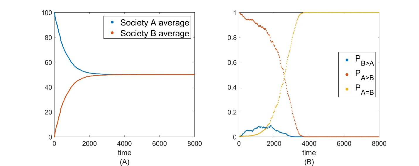
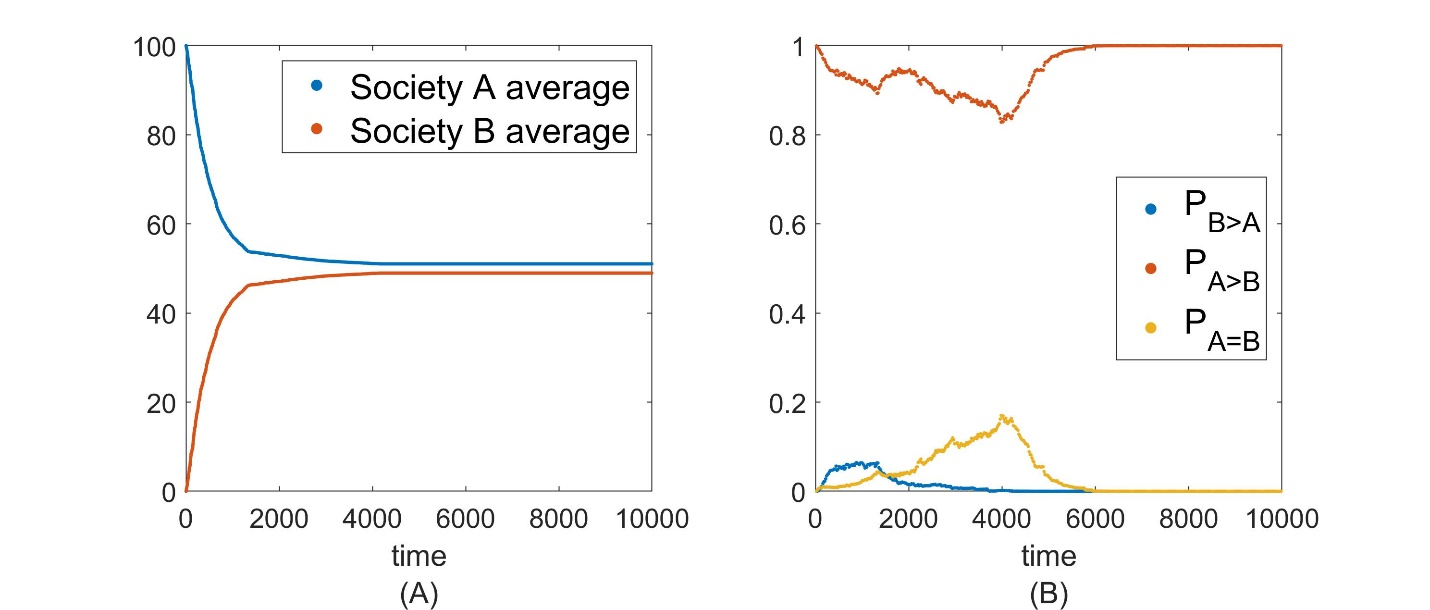
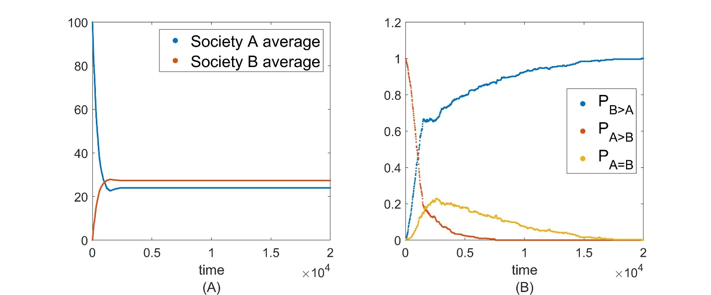
Ordinary Convergence: Because the two societies in the model start out at opposite extremes on the opinion spectrum, \(\overline{A} = 100\), \(\overline{B} = 0\), and because the mechanism governing the assimilation of opinions involves, informally speaking, nothing more than repeatedly grabbing small handfuls of agents and averaging their opinions, one might naturally assume that as time progresses the only large-scale dynamical movement that one will observe will be a very steady, uniform convergence of opinions both between and within the two societies: As seen in Figure 2(A), in this scenario one anticipates that \(\overline{A}\) will decrease and \(\overline{B}\) will increase as they approach the same asymptotic opinion value. Correspondingly, as seen in Figure 2(B), as the two societies converge the probability \(P_{A = B}\) will gradually rise from 0 to 1, while \(P_{A > B}\) will drop from its initial value of 1 towards 0. Probability \(P_{B>A}\) is initially at 0 and will undergo a transient rise before eventually dropping back towards 0 as the societies converge. Figure 3 again illustrates ordinary convergence of opinions between the two societies, except this time the number of inter-society visits that agents are allowed to make has been capped at a small value. In this case, inter-societal assimilation ceases once the caps have been reached, and hence the close convergence in opinions seen in Figure 2(A) never quite reaches completion: In particular, observe in Figure 3(A) that \(\overline{A}\), \(\overline{B}\) will again approach one another (just as in Figure 2(A)) but now their final asymptotic values remain distinct. Regardless, both Figure 2 and Figure 3 illustrate the straightforward convergence of societal opinions that one expects from ordinary assimilation based on simple opinion averaging.
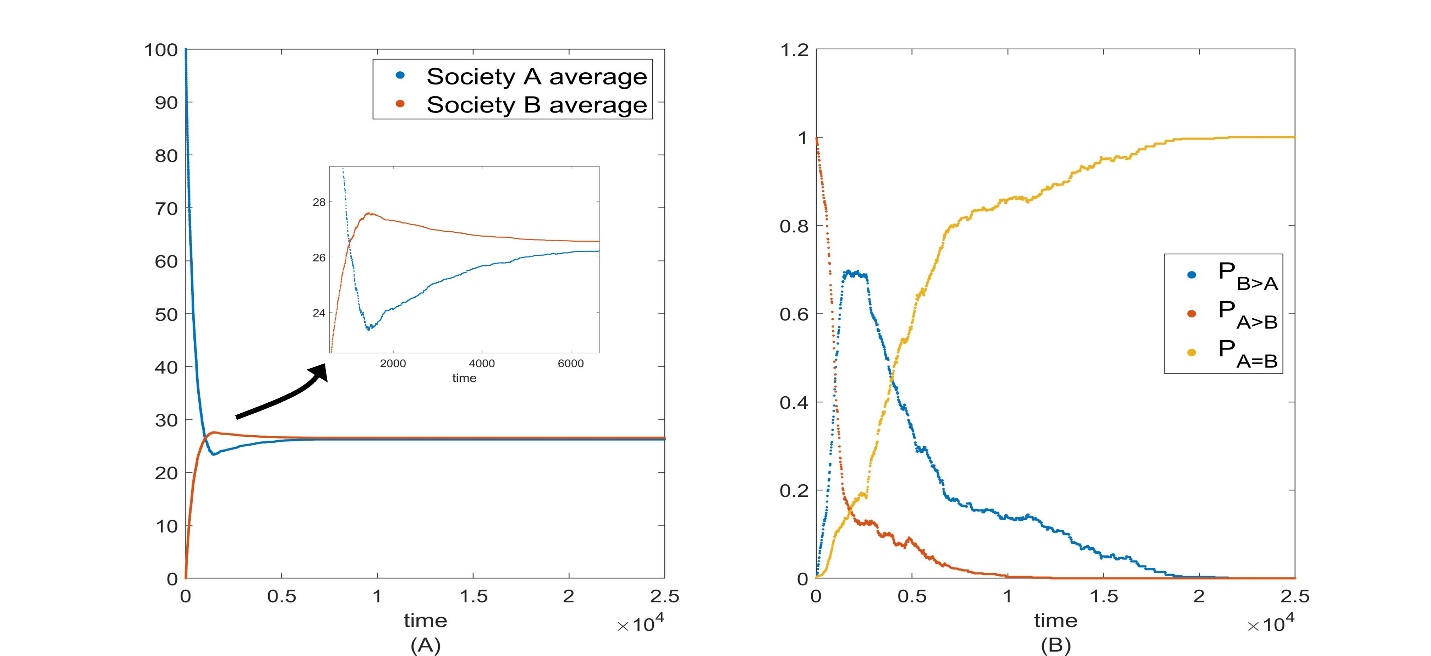
Assimilation Anomaly: While simple opinion averaging does indeed frequently produce the anticipated outcomes shown in Figures 2 and 3, surprisingly this is not the only possibility, as seen in Figure 4. Figure 4(A) shows an example of an assimilation anomaly, wherein at the start of the simulation the average opinion in Society \(A\) is higher than that in Society \(B\), i.e., \(\overline{A} > \overline{B}\), yet at some point in their temporal evolution there is a reversal in the relative positions of the two societies on the opinion spectrum, i.e., \(\overline{A}\) becomes less than \(\overline{B}\). (Again, what makes this large-scale reversal remarkable is that during the local interactions among agents (as described by Equation 1), all agents in the interacting group simply move closer to their group average while preserving their relative ordering on the opinion spectrum. Yet when this local order-preserving rule ( 1) is applied repeatedly to small groups of agents in the two societies, in the aggregate it can produce a large-scale reordering (i.e., reversal) of the average opinion of the two societies even though reorderings are forbidden in the local interactions.) Figure 4(B) shows a complementary view of the anomaly in terms of the quantities \(P_{A>B}\), \(P_{B>A}\), \(P_{A = B}\). We remark that instead of strictly defining the anomaly to be when \(\overline{A}< \overline{B}\), we could expand the definition to include any cases in which \(P_{B>A} > 0.5\) at any point in the evolution, i.e., to scenarios in which there is more than a 50% likelihood that a randomly chosen agent in \(B\) has a higher opinion value than a randomly chosen agent in \(A\). We note that the signatures of the anomaly, \(\overline{A} < \overline{B}\) and \(P_{B>A} > 0.5\) , are not equivalent; it is possible that at some intermediate stage in the societal evolutions that \(\overline{A}< \overline{B}\) is not satisfied but that \(P_{B>A} > 0.5\) is satisfied, for instance. We will refer to both of these criteria, \(\overline{A}< \overline{B}\) and \(P_{B>A} > 0.5\) , as signifying the presence of an assimilation anomaly, since one would not naively expect that either would be possible in a simple assimilative averaging scheme of the model (though we will treat the first of these, \(\overline{A} < \overline{B}\), as the primary signature). Figure 5 illustrates the corresponding appearance of the anomaly when the visitation caps are made more stringent (i.e., lowered in value); owing to these caps the inter-societal interactions cease at some point and the reversal in the average opinions in Societies \(A\) and \(B\) can be permanent (e.g., compare Figures 4(A) and 5(A)).
Figures 4 and 5 serve as illustrative examples of the onset and appearance of the assimilation anomaly at particular parameter values. We next describe more general numerical observations about the emergence of the anomaly in the model.
Trends and numerical observations
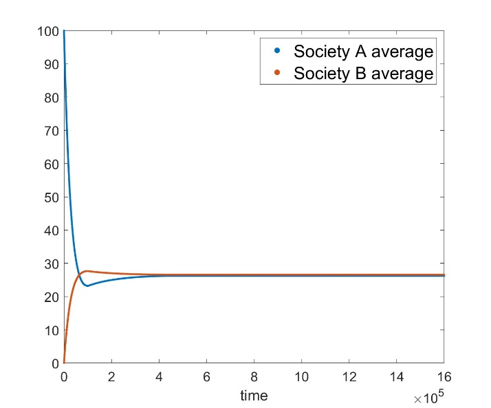
Effect of system size and noise: The emergence of the assimilation anomaly as seen in the preceding figures (Figures 4, 5) is not a result of small system size, nor the result of noise or randomness in the system (e.g., random selection of agents). Figure 6, for instance, illustrates the assimilation anomaly for the same parameter settings used in Figure 4(A) except now the lattice sizes have been increase by a factor of 64 – i.e., \(N_{A} \times N_{A}\) has been increased from \(15 \times 15=225\) agents to \(120 \times 120=14,400\) agents, and \(N_{B} \times N_{B}\) from \(25 \times 25=625\) agents to \(200 \times 200=40,000\) agents. We see no substantive change in the anomaly despite this 64-fold increase in lattice size. Likewise, the only probabilistic element in our model (i.e., the random selection of groups of agents) also proves not to be an essential factor in the emergence of the anomaly. Indeed, as we will describe in Section 4, one can readily create a purely deterministic analog of the assimilation model with arbitrarily large system sizes and the effect will still emerge. The anomaly is not a system-size nor noise-induced phenomenon. Rather, it is a manifestation of the fact that the process of repeated local averaging over small groups of agents can produce overall reversals of opinions in the aggregate.
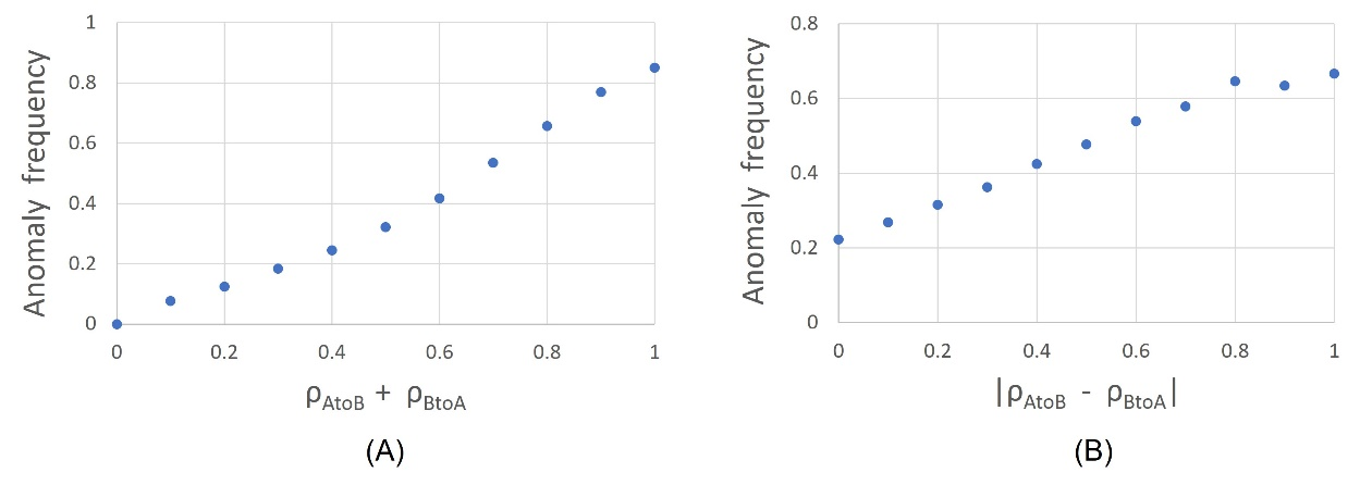
Frequency & magnitude of the assimilation anomaly and parameter dependence: Although an assimilation anomaly can emerge via simple averaging of local group opinions, one might naturally ask how frequently an anomaly occurs compared to the much more familiar and ordinary convergence of opinions seen in Figures 2(A), 3(A). To assess this, we conducted a large-scale numerical exploration across the parameter landscape of the model, varying \(\rho_{A}, \rho_{B}, \rho_{AtoB}, \rho_{BtoA}\) from 0 to 1 in steps of 0.1 (subject to the constraint that \(\rho_{A} + \rho_{B} + \rho_{AtoB} + \rho_{BtoA} = 1\)), allowed \(N_{A}, N_{B}\) to be 15, 20, 25 (i.e., the number of agents in each society could be 225, 400, or 625, meaning that the ratio of system sizes \(\frac{N_{A}^{2}} {N_{B}^{2}}\) could take on nine distinct values ranging from 0.36 to 2.78); let the visitation caps maxBtoA and maxAtoB range from 0,1,2,3; and set the assimilation parameter s to be 0.9 and the numerical tolerance to be 1. Altogether this constitutes 41,184 different parameter scenarios. We found that the assimilation anomaly (defined here as \(\overline{A}< \overline{B}\)) occurs in slightly over one third of these cases. If we restrict consideration to “large” anomalies, arbitrarily defined here as when there is a greater than 2% reversal on a 100-point opinion scale (i.e., when \(\overline{B} - \overline{A} > 2\) ), then we find that these occur in about 15% of the cases. Importantly, we find that assimilation anomalies tend to be more common when the overall rate of inter-societal interactions (as measured by \(\rho_{AtoB} + \rho_{BtoA}\)) is high compared to the intra-societal interaction rate. This is illustrated in Figure 7(A). (See also Figure 7(B) for a related result showing the effect of asymmetry in the inter-societal interaction rates, \(|\rho_{AtoB} - \rho_{BtoA}|\).)
Numerical observations also show that the very largest magnitude assimilation anomalies (e.g., \(\overline{B} - \overline{A} > 13\), which constitute the top 1% of cases) arise primarily in situations where either the asymmetry between the two inter-societal visitation rates is most extreme and/or when the intra-societal interaction rates are extremely low (the underlying reason for these tendencies will become apparent from the analysis presented in Section 4). However, we remark here that the interaction parameter settings (e.g., \(\rho_{A}, \rho_{B}, \rho_{AtoB}, \rho_{BtoA}\)) which generate the most extreme anomalies tend to be somewhat unrealistic from a social-modeling perspective. Thus these extreme cases will not be our prime focus, but they will nonetheless prove helpful in informing our general understanding of the emergence of the anomaly.
We remark also that when discussing the size of an anomaly at a given parameter setting one must bear in mind that the anomaly’s amplitude will vary from run to run since our model contains probabilistic elements. To illustrate, we computed the standard deviation of the anomaly size for 100 runs at a given parameter setting; we repeated this for three different parameter settings each associated with a different anomaly size. At parameter settings (\(\rho_{A}, \rho_{B}, \rho_{AtoB}, \rho_{BtoA}\), \(N_{A}\), \(N_{B}\), maxAtoB, maxBtoA, \(s\), \(tolerance\)) = (0.1, 0.1, 0.1, 0.7, 15, 25, 2, 1, 0.9, 1), a rather large anomaly is observed with average value 8.1 and standard deviation 0.9 (i.e., \(\sim\) 11% variations). At parameter settings (0.3, 0.1, 0.3, 0.3, 15, 25, 1, 1, 0.9, 1) we find anomaly size 2.4 \(\pm\) 0.4 (i.e., \(\sim\) 17% variations). Parameter settings (0.4, 0.3, 0.1, 0.2, 15, 25, 2, 2, 0.9, 1) yield 0.034 \(\pm\) 0.027 (i.e., variations \(>\) 80%). In general the fractional fluctuations tend to decrease with anomaly size. In the last example (i.e., anomaly size 0.034 \(\pm\) 0.027) where the average magnitude of the anomaly is very small, we note that the anomaly was altogether absent in 7 of the 100 runs.
Neighborhood size: We examined different versions of the model, in which we varied the number of nearest neighbors with which an agent interacted (in contrast to an agent always interacting with four nearest neighbors when in its own society or with five neighboring agents when visiting the other society, as in the present model). In particular, we examined two extremes – pairwise interactions in which an agent could only interact with a single other agent (either in its own society or in the other society), and one-to-all interactions in which an agent would interact simultaneously with all other agents in its own society or in the other society. Although the anomaly could appear in each of these cases, it was most pronounced in the one-to-all scenario and least pronounced in the case of pairwise interactions. Hence it is appropriate to think of the assimilation anomaly as being enhanced by multi-agent interactions. The underlying reason for this will become clearer when we consider the analogous heat-diffusion model in the next section.
Visitation caps: One of the main effects of visitation caps was noted previously in comparing Figure 2 to Figure 3, and Figure 4 to Figure 5. Here, we add that although the anomaly can arise both in systems with low caps and in systems with high or no caps, we observed a general tendency for the magnitude of the anomaly to be diminished as the size of the caps was raised.
Other observations: (i) The effect of varying the assimilation parameter s was relatively straightforward: In particular, lowering s tended to slow the overall rate of convergence, as could be anticipated since during each local interaction a reduced s meant that the agents took smaller steps towards their group average (see Equation 1), thereby dilating the overall timescale of the dynamical convergence process. However, if s was reduced significantly without simultaneously raising the visitation caps, then the anomaly would not be seen since the low caps would cause the inter-societal interactions to cease before an anomaly had sufficient time to develop. (ii) The choice of numerical tolerance used in the model, by design, had no effect model’s actual dynamical behavior, though it did affect the qualitative appearance of the \(P_{A>B}\), \(P_{B>A}\), \(P_{A = B}\) plots (e.g., Figures 2(B), 3(B), 4(B), 5(B)) in a straightforward manner. (iii) In general, the presence of asymmetries between the two societies (e.g., in their sizes, in their intra-societal interaction rates, etc.) tended to enhance the size of the observed assimilation anomalies. However, we do note that assimilation anomalies could still emerge even in the case of perfectly symmetric parameter settings, albeit these anomalies tended to be smaller in amplitude and occurred less frequently.
Origin and Analysis of the Assimilation Anomaly
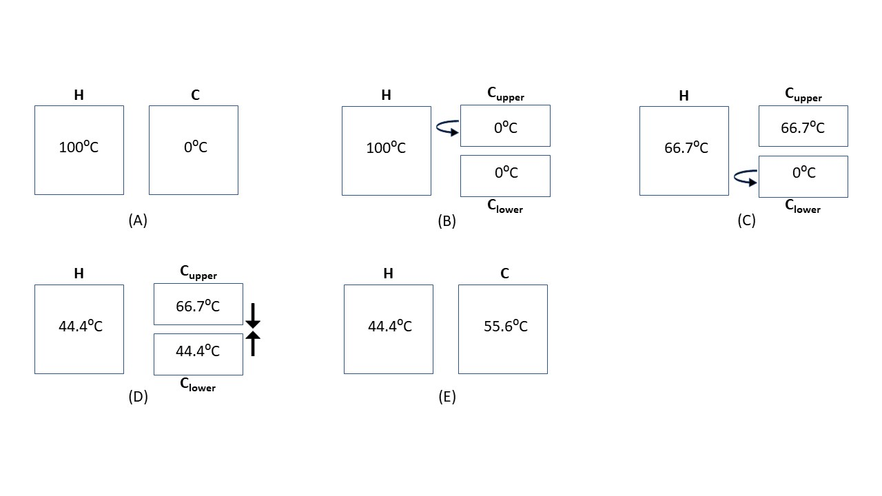
The assimilation anomaly has a simple origin, albeit one that can be easily overlooked in opinion-dynamics models which often have many important bells and whistles attached. The key insight comes from considering a familiar elementary physics scenario involving heat diffusion: Here, rather than two societies, we consider instead the two physical objects shown in Figure 8, labeled \(H\) and C. Object \(H\) is initially hot (say at temperature \(T_{H} = 100 ^\circ C\)) and Object \(C\) is initially cold (\(T_{C} = 0 ^\circ C\)). Apart from their initial temperatures, assume that these objects are identical in all physical characteristics (i.e., same mass, chemical composition, specific heat, etc.). If we were to simply place these two objects in direct thermal contact with one another, their temperatures would start converging (in a straightforward, uneventful manner) towards their average, reaching a final equilibrium value of \(T_{equilibrium} = 50 ^\circ C\). This is just a simple consequence of heat flow and energy conservation, and there are no surprises or subtleties occurring along the way (analogous to the steady convergence seen in Figure 2(A)). So the question becomes, what could we do differently to somehow create a temperature reversal, wherein the final temperature of the initially cold object winds up being higher than the final temperature of the initially hot object? The answer turns out to be deceptively simple: At the start, divide the cold object \(C\) into two equal halves, labeled \(C_{upper}\) and \(C_{lower}\), as shown in Figure 8. Now take the upper half \(C_{upper}\) and put it in thermal contact with hot object \(H\) until their temperatures equilibrate, and afterwards remove \(C_{upper}\) and isolate it. Next take the lower half \(C_{lower}\) and put it in contact with \(H\) until they equilibrate, and then and isolate it. Lastly, put \(C_{upper}\) and \(C_{lower}\) in thermal contact with one another until they equilibrate. At the end of this simple sequential process, we find a straightforward yet still interesting final result: The final temperature of Object \(H\) will be \(44.4 ^\circ C\), whereas the final temperature of Object \(C\) (after its two halves have been recombined) will be \(55.6 ^\circ C\). Indeed, a temperature reversal has been created, in which the two objects have swapped relative positions on the temperature spectrum, with the initially hot object ending up at a lower temperature than the initially cold object. This reversal occurs even though ordinary heat diffusion (here, applied to multiple objects in succession) involves nothing more than taking simple averages in succession, and we normally (albeit incorrectly) think of local serial averaging as inevitably leading to steady global convergence, rather than being capable of producing any sort of large-scale reversals. This simple heat diffusion paradigm provides a key physical insight into the assimilation anomaly.
Although the above heat-diffusion scenario represents a highly simplified – indeed somewhat oversimplified – analog of what is actually occurring in our opinion-dynamics model, it nevertheless does correctly capture the essential process at the heart of the assimilation anomaly. Let’s now tighten the connection by considering a slightly more sophisticated heat diffusion scenario to make it correspond a bit more closely to the assimilative mechanism in our opinion-dynamics model. We will again start with two physically similar objects at different initial temperatures \(T_{H}\) and \(T_{C}\), though this time allow for the possibility that they have different masses \(M_{H}\) and \(M_{C}\) in order to better align with the prospect that the two societies \(A\) and \(B\) in our assimilation model might contain different numbers of agents. Now, however, rather than dividing up object \(C\) into just two pieces and sequentially placing them in thermal contact with \(H\) (as was done in Figure 8), we will instead divide up object \(C\) into a very large number of small pieces, and then successively bring each piece into temporary contact with object \(H\) before eventually recombining all the small bits of \(C\) back together. See Figure 9. In this scenario each small piece of \(C\) will play a role analogous to an individual agent in Society \(B\) making a visit to Society \(A\). The heat flow calculation is straightforward.
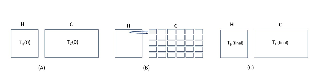
Let \(T_{H}(t)\) and \(T_{C}(t)\) denote the respective temperatures of objects \(H\) and \(C\) at time \(t\), with \(T_{H}(0)\) and \(T_{C}(0)\) denoting their initial temperatures. We break object \(C\) into small, equal-size bits of mass \(\Delta M_{C}\) each at temperature \(T_{C}(0)\). Note that the total number of such bits is \(\frac{M_{C}}{\Delta M_{C}}\). Next discretize time \(t = 0, \Delta t, 2 \Delta t, 3 \Delta t, \dots, \frac{M_{C}}{\Delta M_{C}} \Delta t\), where at each time step \(\Delta t\) one small piece of mass, \(\Delta M_{C}\), is put into contact with object \(H\) and (instantaneously) thermally equilibrates with it, and then this small piece is removed and set aside. Then another small bit \(\Delta M_{C}\) is brought over to \(H\), etc., etc. This sequential process repeats until all the pieces of \(C\) have in turn equilibrated with \(H\) (the total elapsed time will be \(t_{final} = \frac{M_{C}}{\Delta M_{C}} \Delta t\)). Note that when a new bit of \(C\) is brought over at time \(t\), the updated temperature of \(H\) will be:
| \[ T_{H}(t + \Delta t) = \frac{M_{H} T_{H}(t) + \Delta M_{C} T_{C}(0)}{M_{H} + \Delta M_{C}}\] | \[(5)\] |
| \[ T_{H}(t + \Delta t) = T_{H}(t) + \frac{\Delta M_{C}}{M_{H}}(T_{C}(0) - T_{H}(t))\] | \[(6)\] |
Rewriting, we have:
| \[ \frac{T_{H}(t + \Delta t) - T_{H}(t)}{\Delta t} = \frac{R}{M_{H}}(T_{C}(0) - T_{H}(t))\] | \[(7)\] |
| \[ T_{H}(t_{final}) = T_{C}(0) + (T_{H}(0) - T_{C}(0))e^{-\frac{M_{C}}{M_{H}}}\] | \[(8)\] |
| \[T_{C}(t_{final}) = \frac{M_{H}}{M_{C}} T_{H}(0) + (1 - \frac{M_{H}}{M_{C}}) T_{C}(0) - \frac{M_{H}}{M_{C}} (T_{H}(0) - T_{C}(0))e^{-\frac{M_{C}}{M_{H}}}\] | \[(9)\] |
From an examination of the above expressions, one can show that \(T_{C}(t_{final}) - T_{H}(t_{final}) > 0\), meaning that, under this scenario, heat diffusion will always produce a reversal of relative positions of the two objects on the temperature spectrum, i.e., the process of repeatedly thermal averaging object \(H\) with small pieces of object \(C\) yields an overall temperature reversal wherein the initially hot object \(H\) winds up at a lower final temperature than that of the initially cold object \(C\). For the case of equal masses, for instance, we find that the magnitude of the temperature reversal is \(T_{C}(t_{final}) - T_{H}(t_{final}) = (1 - \frac{2}{e})(T_{H}(0) - T_{C}(0))\), i.e., about 26.4% of the initial temperature difference. A simple calculation shows that the mass ratio that maximizes the size of the temperature reversal is \(\frac{M_{C}}{M_{H}} \approx 1.793\); in this case the magnitude of the temperature reversal is approximately 29.8% of the initial temperature difference. We also mention that in the limit that one of the two objects is much more massive than the other (i.e., either \(M_{C} \ll M_{H}\) or \(M_{C} \gg M_{H}\)) then the magnitude of the temperature reversal diminishes to 0.
The heat diffusion process described above is at the core of what is producing the assimilation anomaly in the opinion-dynamics model. Both the heat diffusion scenario and our simple assimilation scheme rely on nothing more than repeatedly taking local averages (over subcomponents of objects in the former case and over small groups of agents in the latter case). The essential point is that even though the local averaging process itself can only produce local convergence (of temperatures and/or of opinions) without any overshooting or reordering, by repeatedly taking local averages one can create a large-scale reversal in the aggregate, i.e., an assimilation anomaly.
Several comments are in order.
We first point out that while the above heat diffusion analysis has provided the basic physical and mathematical insight into the assimilation anomaly, nonetheless there are some key technical differences between the opinion-dynamics model and the heat diffusion examples:
- In the opinion-dynamics model we allowed for individual agents from both societies \(A\) and \(B\) to make visits to the other society, whereas in our heat diffusion illustration we only divided one of the two objects (specifically, object \(C\)) into small (agent-like) bits and allowed these bits to sequentially “visit” object \(H\), but we did not also divide object \(H\) into bits and allow these to visit object \(C\). (Later we will extend the heat model to account for two-way visitations.) This asymmetric visitation in the above heat diffusion scenario corresponds to setting the visitation rate \(\rho_{AtoB}\) from Society \(A\) to Society \(B\) to 0 in the opinion-dynamics model. Importantly, as we will show later, the question of asymmetric versus symmetric visitation proves unimportant, since either case can give rise to an assimilation anomaly.
- In the heat diffusion scenario of Figure 9 each small piece of object \(C\), when brought over to object \(H\), thermally equilibrates with the whole of \(H\), whereas in our opinion-dynamics model a visiting agent only directly interacts with (and averages with) a small group of agents residing within some local neighborhood of the other society. This is a critical, nontrivial difference between the heat diffusion and assimilation scenarios. We can garner insight into the implications of this distinction by comparing the two heat diffusion scenarios described above – the first in which object \(C\) was simply divided in half (Figure 8), and the second where it was divided into a large number of pieces (Figure 9). A calculation shows that the size of the temperature reversal is larger in the latter case. This has direct implications for our assimilation model: it suggests that having a single agent interact with a larger number of agents in the other society will produce a bigger effect than having an agent only interact with a small group of agents residing in some local neighborhood of the other society. This observation is consistent with the numerical trend described previously, i.e., the assimilation anomaly will be magnified as the number of agents in a local neighborhood is increased. We can thus think of the preceding calculation for the size of this thermal anomaly (i.e., 29.8% of the initial temperature differential) as providing a theoretical upper bound on the size of the assimilation anomaly under one-way visitations, since as argued above averaging over a smaller neighborhood size in the assimilation model compared to the thermal case will reduce the anomaly’s magnitude below this theoretical limit. Our numerical simulations confirm this.
- In the heat diffusion scenario, each time a small bit of Object \(C\) was brought over to Object \(H\) we assumed that the thermal equilibration process within both that small bit of \(C\) and the whole of \(H\) was virtually instantaneous, whereas in the opinion-dynamics model we allowed for the possibility of incomplete equilibration by introducing an assimilation parameter s which could be set to be less than one. (Recall that when \(s=1\) all agents in interacting group immediately adopt the average group opinion whereas when \(s < 1\) each interacting agent only moves partway closer to the group average.) One can think of the \(s < 1\) case as corresponding to a heat-diffusion situation in which the thermal conductivity of objects \(C\) and \(H\) are finite resulting in partial rather than full equilibration. This in turn tells us what to expect: as the assimilation parameter \(s\) is reduced, timescales for equilibration increase, and the size of the anomaly will tend to diminish. This is precisely what was numerically observed in our earlier simulations.
- In the heat diffusion scenario of Figure 9, after each small piece of Object \(C\) was placed in thermal contact with Object \(H\) it was then removed and not permitted to have any further interactions with Object \(H\). This is analogous to setting the inter-society visitation cap equal to one in our assimilation model. The question thus becomes, what happens if we raise the visitation cap in the assimilation model? We again can turn to the thermal diffusion scenario for insight: Raising the visitation cap corresponds to allowing the small bits of Object \(C\) to visit Object \(H\) multiple times. But with each successive visit the temperature of a small piece of \(C\) will become closer to that of \(H\), which will therefore tend to reduce the magnitude of the final aggregate temperature reversal. Hence we can anticipate that, all else being equal, the size of the assimilation anomaly (at least in the case of asymmetric visitations) should generally be reduced as the visitation caps are increased. This finding is consistent with the overall numerical trends observed previously (though, as a cautionary remark, we note that this general trend is not an inviolable rule). As a side remark, we do wish to note that the above correspondence between the visitation caps in the assimilation model and the heat diffusion scenario is still slightly imperfect: In the thermal diffusion scenario, after each bit of Object \(C\) interacted with Object \(H\) it was then removed and isolated not only from \(H\) but from the rest of \(C\) as well (until the very end when all of the small pieces of \(C\) were recombined). But in the assimilation model, an agent, after visiting the other society and returning home is allowed to interact with its neighbors, i.e. it is not isolated. This difference between the heat diffusion scenario and the assimilation scenario means that one cannot in general fully map these two models directly onto one another. Nonetheless, the underlying physical process at work in the heat diffusion scenario does provide the correct physical justification for why raising visitation caps will tend to reduce the magnitude of the reversal in overall societal opinions.
Despite the differences, the dynamical mechanism responsible for the temperature reversal in the heat diffusion case is nearly identical to that responsible for the large-scale reversal of societal opinion in the assimilation case. Indeed, we point out that we can rigorously map the above heat diffusion scenario onto the assimilation model under the following circumstances: If in the assimilation model we set \(\rho_{AtoB} = 0\), \(\rho_{B} = 0\), \(s=1\), maxBtoA \(= 1\), and increase the neighborhood sizes on the societal lattices from just four nearest neighbors to the entirety of the lattice (thereby creating one-to-all interactions), then the two scenarios rigorously match one another. We have carried out numerical simulations of the assimilation model under these extreme conditions and have confirmed that they agree with the preceding theoretical predictions of \(T_{H}(t_{final})\), \(T_{C}(t_{final})\) computed for the thermal diffusion case.
We noted earlier that it is possible to extend the above thermal diffusion scenario of Figure 9 to better mimic the two-way visitations of the assimilation model. Here, one again considers two objects, one initially hot and one initially cold (for ease we assume they have the same mass \(M\)). This time, however, we divide both objects up into small pieces of mass \(\Delta M\), and simultaneously bring a small bit of mass from the cold object to the hot object and a small bit of mass from the hot object to the cold. After each has thermally equilibrated we return each piece to its respective side (but keep it isolated). We repeat this process until all bits of both objects have thermally “visited” and returned. We then allow all the small bits from the originally cold side to recombine and equilibrate, and similarly recombine and equilibrate all the bits from the originally hot side. We again find that an overall temperature reversal will occur. The resulting heat flow calculations describing this process are still analytically tractable albeit slightly more involved than the previous one-way visitation case (since they entail constructing and solving two coupled non-autonomous differential equations, which can be readily done via a judicious change of variables). We omit the details of this calculation and instead highlight the main qualitative and quantitative findings: Most importantly we find that these two-way visitations produce a temperature reversal, with \(T_{C}(t_{final}) - T_{H}(t_{final}) = \frac{1}{3}(T_{H}(0) - T_{C}(0)) > 0\). In other words, the temperature reversal that was found in the previous thermal diffusion scenario (Figure 9) was not caused by the asymmetric, one-way nature of the visitations in that scenario, but rather also similarly emerges with two-way thermal visitations. This is why, in our assimilation model, we numerically observed the presence of the anomaly regardless of whether we set one of the inter-societal visitation rates (either \(\rho_{AtoB}\) or \(\rho_{BtoA}\)) to zero (i.e., one-way visitations) or not (i.e., two-way visitations). On a technical note, we mention that even this more elaborate two-way thermal diffusion scenario still does not allow for a completely general one-to-one matching onto our opinion-dynamics model for several reasons. For instance, our assimilation model includes additional adjustable features that the thermal model lacks (e.g., in the assimilation model we can independently select values for \(\rho_{A}\), \(\rho_{B}\), \(\rho_{AtoB}\), \(\rho_{BtoA}\) respectively, whereas the thermal model lacks this flexibility). Additionally, as previously noted, in the heat-diffusion model, after each piece returns to its original side it remains thermally isolated from the other pieces until the very end, whereas in the assimilation model a visiting agent returns home is not kept isolated. Despite these nominal differences, the key mechanism responsible for these large-scale reversals (in temperature in the heat diffusion example or in societal opinion in the assimilation model) remains nearly identical.
From our heat diffusion analysis we can now understand a crucial aspect of the assimilation anomaly which was briefly noted in Sections 2 and 3: The reversal of the overall positions of two societies along the opinion spectrum is not the result of a fluctuation arising from noise or randomness in the system (e.g., random selection of agents), nor is it a result of small system size. Rather, the heat diffusion analysis demonstrates that the analogous anomaly similarly arises in a purely deterministic system of arbitrarily large size (i.e., recall that in the thermal diffusion examples there were no probabilistic elements and no restrictions on the system sizes). In short, the anomaly is a manifestation of the fact that the process of repeated local averaging over small groups of agents can produce overall reversals of opinions in the aggregate (and is not associated with fluctuations or small system sizes).
Lastly, we remark that the preceding heat diffusion analysis could readily be extended further by allowing for the two objects at different starting temperatures to also have different specific heats. In terms of the opinion-dynamics model, this would alter the inter-societal interactions somewhat, and would correspond to a situation in which the interacting agents from the two societies have differing levels of intrinsic “stubbornness” in their opinions (or, equivalently, exert different levels of influence on one another). In this scenario, the differing specific heat values would correspond to taking weighted numerical averages of the interacting agents’ opinions, rather than simple numerical averages. Nonetheless, even if the model were extended in this way, we would still expect that the assimilation anomaly could emerge (at appropriate parameter settings) just as before.
Concluding Remarks
The goal of this paper was a relatively modest one – to highlight the existence of a simple yet interesting dynamical phenomena associated with assimilation that can arise even in the most basic of social-influence models. We described an assimilation anomaly wherein two societies that start out on opposite ends of an opinion spectrum can reverse their relative positions through a simple opinion-averaging process. What makes this phenomenon surprising is that it arises even in the most elementary assimilation scheme imaginable that entails nothing more than allowing small groups of agents in the two societies to interact and average their opinions. During these local interactions each agent simply takes a step towards the group average, and the agents can never pass one another on the opinion spectrum during an interaction. Although one might casually presume that this ordinary numerical averaging of opinions could only produce a steady, inevitable convergence of overall societal opinions, we instead illustrated how a simple local averaging process – when applied repeatedly to different small groups of agents across the two societies – can lead to a global reversal in the average opinions of the two societies. A straightforward heat-diffusion model from physics provides the mathematical underpinnings and physical intuition behind the anomaly. This finding involving two interacting societies is notably distinct from other interesting dynamical phenomena that have been previously observed within a society in various social-influence models (e.g., fragmentation, polarization, phase transitions, etc.). Lastly, we mention that in this work we have, quite intentionally, shied away from attempting to directly match our model’s findings to specific real-world data drawn from any particular case study, since to do otherwise would be misleading. The reason is clear: realistic modelling of the transmission and evolution of opinions across human societies requires relatively sophisticated opinion-dynamics models that incorporate a large number of distinct, sociologically motivated, dynamical mechanisms. Our present model, in contrast, is focused exclusively on a single such mechanism – a local numerical averaging process to mimic assimilation – to illustrate a particular point. In particular, it serves as an illustrative reminder that as one builds increasingly complex numerical models to simulate social interactions, it is crucial to fully understand the behavior of each of the various dynamical processes that one incorporates into the model. What we have shown here is that even one of the simplest possible of such processes – using local averaging as a basic mechanism to model assimilation of opinions - can yield some surprises.
References
ABELSON, R. P. (1964). Mathematical models of the distribution of attitudes under controversy. In N. Frederiksen & H. Gulliksen (Eds.), Contributions to Mathematical Psychology. New York, NY: Rinehart Winston.
AXELROD, R. (1997). The dissemination of culture: A model with local convergence and global polarization. Journal of Conflict Resolution, 41(2), 203–226. [doi:10.1177/0022002797041002001]
CASTELLANO, C., Fortunato, S., & Loreto, V. (2009). Statistical physics of social dynamics. Review of Modern Physics, 81, 591. [doi:10.1103/revmodphys.81.591]
CASTELLANO, C., Marsili, M., & Vespignani, A. (2000). Nonequilibrium phase transition in a model for social influence. Physical Review Letters, 85, 3536. [doi:10.1103/physrevlett.85.3536]
CURRIN, C. B., Vera, S. V., & Khaledi-Nasab, A. (2022). Depolarization of echo chambers by random dynamical nudge. Scientific Reports, 12(1), 1–13. [doi:10.1038/s41598-022-12494-w]
DALEY, D. J., & Kendall, D. G. (1964). Epidemics and rumors. Nature, 204, 1118.
DITTMER, J. C. (2001). Consensus formation under bounded confidence. Nonlinear Analysis, 47, 4615–4621. [doi:10.1016/s0362-546x(01)00574-0]
FENNELL, S. C., Burke, K., Quayle, M., & Gleeson, J. P. (2021). Generalized mean-field approximation for the deffuant opinion dynamics model on networks. Phys. Rev. E, 103, 012314. [doi:10.1103/physreve.103.012314]
FLACHE, A., & Macy, M. W. (2011). Local convergence and global diversity: From interpersonal to social influence. Journal of Conflict Resolution, 55(6), 970–995. [doi:10.1177/0022002711414371]
FRIEDKIN, N., & Johnsen, E. (2011). Social Influence Network Theory: A Sociological Examination of Small Group Dynamics. Cambridge: Cambridge University Press. [doi:10.1017/cbo9780511976735]
GANDICA, Y., Medina, E., & Bonalde, I. (2013). A thermodynamic counterpart of the axelrod model of social influence: The one-dimensional case. Physica A: Statistical Mechanics and Its Applications, 392(24), 6561–6570. [doi:10.1016/j.physa.2013.08.033]
HEGSELMANN, R., & Krause, U. and. (2002). Opinion dynamics and bounded confidence models, analysis, and simulation. Journal of Artificial Societies and Social Simulation, 5(3), 2.
KEIJZER, M. A., & Mäs, M. (2022). The complex link between filter bubbles and opinion polarization. Data Science, 5(2), 139–166. [doi:10.3233/ds-220054]
KEIJZER, M. A., Mäs, M., & Flache, A. (2018). Communication in online social networks fosters cultural isolation. Complexity, 2018, 9502872. [doi:10.1155/2018/9502872]
KLEMM, K., Eguíluz, V. M., Toral, R., & San Miguel, M. (2003). Global culture: A noise-induced transition in finite systems. Physical Review E, 67, 045101. [doi:10.1103/physreve.67.045101]
KRAUSE, U. (2000). A discrete nonlinear and non - autonomous model of consensus formation. In S. Elaydi, G. Ladas, J. Popenda, & J. Rakowski (Eds.), Communications in Difference Equations (pp. 227–236). Amsterdam: Gordon and Breach.
KUPERMAN, M. N. (2006). Cultural propagation on social networks. Physical Review E, 73, 046139.
LORENZ, J. (2007). Continuous opinion dynamics under bounded confidence: A survey. International Journal of Modern Physics C, 18(2), 1819–1838. [doi:10.1142/s0129183107011789]
NGUYEN, N., Chen, H., Jin, B., Quinn, W., Tyler, C., & Landsberg, A. S. (2021). Cultural dissemination: An agent-Based model with social influence. Journal of Artificial Societies and Social Simulation, 24(4), 5. [doi:10.18564/jasss.4633]
PARISI, D., Cecconi, F., & Natale, F. (2003). Cultural change in spatial environments: The role of cultural assimilation and internal changes in cultures. Journal of Conflict Resolution, 47(2), 163–179. [doi:10.1177/0022002702251025]
PERALTA, A. F., Kertész, J., & Iñiguez, G. (2023). Opinion dynamics in social networks: From models to data. In T. Yasseri (Ed.), Handbook of Computational Social Science. Edward Elgar Publishing Ltd: Cheltenham.
PERES, L. R., & Fontanari, J. F. (2012). Effect of external fields in Axelrod’s model of social dynamics. Physical Review E, 86, 031131. [doi:10.1103/physreve.86.031131]
PFAU, J., Kirley, M., & Kashima, Y. (2013). The co-evolution of cultures, social network communities, and agent locations in an extension of Axelrod’s model of cultural dissemination. Physica A: Statistical Mechanics and Its Applications, 392(2), 381–391. [doi:10.1016/j.physa.2012.09.004]
PINEDA, M., Toral, R., & Hernández-García, E. (2009). Noisy continuous-opinion dynamics. Journal of Statistical Mechanics: Theory and Experiment, 2009. [doi:10.1088/1742-5468/2009/08/p08001]
REIA, S. M., & Fontanari, J. F. (2016). Effect of long-range interactions on the phase transition of Axelrod’s model. Physical Review E, 94, 052149. [doi:10.1103/physreve.94.052149]
RODRÍGUEZ, A., del Castillo, M., & Vázquez, G. (2009). Induced monoculture in Axelrod model with clever mass media. International Journal of Modern Physics C, 18(20), 1233–1245. [doi:10.1142/s012918310901431x]
SHIBANAI, Y., Yasuno, S., & Ishiguro, I. (2001). Effects of global information feedback on diversity: Extensions to Axelrod’s adaptive culture model. Journal of Conflict Resolution, 45(1), 80–96. [doi:10.1177/0022002701045001004]
SIRBU, A., Loreto, V., Servedio, V. D. P., & Tria, T. (2016). Opinion dynamics: Models, extensions and external effects. In V. e. Loreto (Ed.), Participatory Sensing, Opinions and Collective Awareness. Berlin Heidelberg: Springer.
STIVALA, A., & Keeler, P. (2016). Another phase transition in the Axelrod model. arXiv preprint. Available at: https://arxiv.org/abs/1612.02537
VAZQUEZ, F., González-Avella, J. C., Eguíluz, V. M., & San Miguel, M. (2007). Time-scale competition leading to fragmentation and recombination transitions in the coevolution of network and states. Physical Review E, 76, 046120. [doi:10.1103/physreve.76.046120]
VESPIGNANI, A. (2011). Modelling dynamical processes in complex socio-technical systems. Nature Physics, 8, 32–39. [doi:10.1038/nphys2160]
WEISBUCH, G., Deffuant, G., Amblard, F., & Nadal, J. (2002). Meet, discuss, and segregate! Complexity, 7(3), 55–63. [doi:10.1002/cplx.10031]
XIA, H., Wang, H., & Xuan, Z. (2011). Opinion dynamics: A multidisciplinary review and perspective on future research. International Journal of Knowledge and Systems Science, 2(4), 72–79. [doi:10.4018/jkss.2011100106]