Calibrating an Opinion Dynamics Model to Empirical Opinion Distributions and Transitions

and
aConstructor University, Germany; bConstructor University Bremen, Germany
Journal of Artificial
Societies and Social Simulation 26 (4) 9
<https://www.jasss.org/26/4/9.html>
DOI: 10.18564/jasss.5204
Received: 13-Feb-2023 Accepted: 05-Jul-2023 Published: 31-Oct-2023
Abstract
Agent-based models of opinion dynamics enable the investigation of societal phenomena that psychological theories of individual opinion change trigger in artificial societies. Many of such models are validated on the phenomenological level only (e.g., can they produce polarization) and not with respect to opinion data about real-world attitude distributions known from social surveys or individual attitude change observed in panel surveys. In this work, we use an existing agent-based model which builds on repeated random pairwise interaction as introduced in many early opinion dynamics models with a function of individual opinion change function that includes the contagious and assimilating opinion adjustment, idiosyncratic opinion change, and motivated cognition, which is a generalization of the concept of bounded confidence. Depending on its parameters, this model creates different opinion distributions. By arguing that institutional trust is formed by an exchange of experiences and opinions, we then match the opinion distributions from the seven institutional trust questions in the European Social Survey to the simulated ones. Goodness-of-fit measures allow to calibrate the model parameters to reproduce 1,235 empirical distributions (for different countries and years) and further on, the calibration procedure is extended to data about individual opinion change from the Swiss Household Panel where participants reported their trust in the government on a yearly basis. Overall the opinion dynamics model reproduces most of the empirical distributions to a high degree, additionally, matching agents to individuals shows also a high level of concordance. In the analysis, we show that the concept of motivated cognition is a crucial part to achieve this level of accuracy. However, in both calibrations, we expose the shortcoming of the model to reproduce individuals with extreme and neutral attitudes.Introduction
Agent-based modeling (ABM) is a mathematical framework that allows to establish various kinds of models. Instead of equations about changes in macroscopic quantities, ABM is using simple behavioral rules at the individual (micro) level to produce aggregated (macro) level phenomena. Many agent-based models are developed in the field of opinion dynamics. However, the behavioral rules in OD models mostly stem from postulated dynamics (Bianchi et al. 2007). The main focus of opinion dynamics models is to grow familiar macro-social patterns, like polarization or consensus, as a way to identify possible causal mechanisms (Epstein & Axtell 1996). Whether a model can reproduce empirical data by tuning and calibrating parameters is rarely considered.
Recently Flache et al. (2017) pointed out that opinion dynamics resulting from social influence is a puzzling phenomenon and, models of social influence lack empirical grounding. Therefore in this paper, we propose methods for calibrating a model of social influence in opinion dynamics to attitude data from surveys and panels and further propose methods for a quantitative analysis.
Historically, the bounded confidence models of Hegselmann & Krause (2002) and Deffuant et al. (2000) illustrated with a simple mechanism how opinions can fragment into clusters. Both of these and various other models have been studied on different communication topologies (Meng et al. 2018) as well as with the inclusion of noise (Pineda et al. 2009) or various variations to the overall dynamic (Sobkowicz 2015). Similar extensions are also made for the many other popular opinion dynamics models like Axelrod (1997), Friedkin & Johnsen (1990), DeGroot (1974) etc. All these models are based on simple and well-understood dynamics which allow integration of empirically observed psychological phenomena like, e.g., confirmation bias (Del Vicario et al. 2017) or echo chambers (Baumann et al. 2020) and study their consequences in regard to the employed model. Over time, many more assumptions on opinion dynamics, different models, and various dynamics were postulated but rarely gain in popularity.
Flache et al. (2017) identified three main micro-mechanisms: assimilative, similarity biased, and repulsive influence. Assimilative influence always describes the mechanism of approaching the opinions of others to a certain degree. Similarity bias excludes this influence to only agents or individuals who are sharing a certain similarity like group membership, with bounded confidence as the main implementation. Repulsive influence describes the ability to dissociate your opinion from, for example, a neutral opinion, by becoming more extreme.
Validating or falsifying these mechanisms and the corresponding models is crucial to enhance the field of opinion dynamics. A universal model that can explain multiple phenomena on the individual (micro) as well as on the aggregated (macro) level is still a distant reality. However, the validation of simple behavioral rules by using experiments or agent-based modeling can establish a foundation for future more complex and viable models.
Why do we want to calibrate models? Macy & Willer (2002) calls for testing its external validity after being familiar with a model and its potential generative capacity. Contrastingly, Axtell et al. (1996) warns to keep in mind, that testing and validating opinion dynamics models still need a lot of work and cannot be as robust as for example a theory in physics. Nevertheless, calibrating models can be the first step and, consequently, increase our understanding of real-world phenomena. If ultimately simulations are able to reproduce empirical macro-social patterns and empirical micro-social dynamics, opinion dynamics models would make a step toward realism.
Troitzsch (2021) established an overview of models (especially one-dimensional ones) and also discloses the lack of empirical validation in the field of opinion dynamic models. He emphasized that Lorenz (2017) was one of the first papers which tried to validate OD models with empirical survey data. This study was a first try and showed the (limited) possibilities to recreate left-right attitude landscapes from the European Social Survey (ESS) with a noisy bounded confidence model inspired from Pineda et al. (2009).
In the recent study Lorenz et al. (2021) developed a model motivated by Hunter et al. (1984) which could recreate structural similarities with attitude landscapes by using simulated data and attitude landscapes found in various topics in the European Social Survey. However, these comparisons were done qualitatively and lacked methods and parameters for a quantitative approach.
Research Design
We use the model of Lorenz et al. (2021) which has parameters to modify how individuals adjust their opinions1. Lorenz et al. (2021) already compare macroscopic model output with empirical attitude distributions from the European Social Survey. However, the comparison remains on the phenomenological level and an attempt to calibrate the model to replicate such data best is a natural next step. Further on, the model is simple enough to allow some understanding of how parameters change the aggregated outcomes.
The model can show the emergence of unimodal and multimodal distribution of attitudes from initially normally distributed opinions. Further on, a bias of the average attitude towards one side can emerge. The stylized outcomes of the model include extreme or central consensus, bipolarization into two extreme modes, as well as fragmented or bell-shaped distributions. In most regions of the parameter space, the model converges towards stochastically stable distributions. That means the shape of the distribution remains stable within narrow ranges of random fluctuation, while individual attitudes keep changing substantially.
Both phenomena – macroscopic stability and individual changes – are also visible in empirical data. Large-scale macroscopic stability of attitude distributions can be observed comparing attitude distributions from different rounds of the European Social Survey (see Gestefeld et al. 2022). The phenomenon of individual changes under a stable macroscopic distribution shows up in the panel data of the Swiss Household panel which will be shown in the following. The commonality of simulation data of the model and empirical data motivates the following replication and calibration study.
We choose institutional trust for this study. We discuss in the following why this is a good topic for opinion dynamics although it is not a typical example used for the motivation of opinion dynamics. Besides this discussion, there are also two more pragmatic reasons. First, the attitude distributions are typically not that complex often showing a unimodal distribution. So, the dynamic phenomenon the model needs to produce is mostly a shift of a unimodal distribution to one side. Second, "Trust in Government" is one of the few attitude variables on an eleven-point scale in the Swiss Household Panel which we can match directly to the many variables about trust in institutions in the European Social Survey.2 Eleven-point scales are more favorable than shorter scales for our purpose of calibrating models of continuous opinion dynamics.
The central research question of this study is: What is the capacity of the model to replicate empirical distributions of trust in institutions for different countries and waves of the European Social Survey?
We will answer this question by calibrating model parameters and comparing aggregated data generated by various simulations to the attitude distributions of institutional trust in the European Social Survey for different countries, rounds, and institutional trust topics. To that end, we define a goodness-of-fit measure to evaluate the difference between simulated and empirical data. Based on this, we also select the best-fitting parameters for each empirical distribution. We do not use any empirical information in the initialization and computation of simulation data. Thus, we try to capture a potential social process that may have formed these real-world attitude landscapes (see Gilbert & Troitzsch 2005).
In contrast to previous research, we will show that the model can produce a stable opinion distribution which then can be compared to empirical distributions. In comparison in most cases, empirical distributions are compared to simulated ones during its "spin-up" time which might just be a preliminary state towards e.g. bipolarization (Duggins 2017).
The second part of this study is to extend the calibration to individual-level data. Here we use the data from the Swiss Household Panel which has annual data from individual data about trust in the government over 11 years. First, the model is calibrated to the attitude distribution on the aggregated level like before.
Then we tackle the second research question of this study: What is the capacity of the model to replicate transition probabilities of individual attitude change as observed in the Swiss Household Panel and do the calibrated parameters match the outcomes of the first research question?
In the next section, we introduce the topic of political trust and different theories that explain the individual evaluation and assessment of political trust from a social science perspective. Then we discuss how these will be incorporated into the agent-based model. Afterward, we present the model and its parameters in more detail and introduce the measures for the goodness-of-fit with empirical data.
Trust in Political Institutions
In this study, we study trust in political institutions, which is a common topic in social surveys. Castiglione et al. (2008) state that "there is a relatively strong consensus in the literature about the importance of political trust. Much less agreement, however, can be found about the theoretical status of the concept, its actual meaning, the causes, and the consequences of political trust." In surveys, the concept of political trust (Zmerli & Hooghe 2011) appears in questions about individual trust in various institutions (like parliaments government, political parties, politicians, the legal system, or the police). The decline of trust in institutions is a common empirical question (Van de Walle et al. 2008).
Theories indicate that a lack of political trust could result in destabilizing democracies and hinder the enforcement of policies (Citrin & Muste 1999), policies which can be life-saving for many people as in recent CoViD-19 pandemic with policies of mask mandates or lockdowns.
From the perspective of opinion dynamics models, we are interested in the capacity of models to show the emergence of trust distributions through social interaction. Hence, we want to introduce two of the major theories which consolidate the causes and the assessment of individual institutional trust.
First, Inglehart (1997) argues that trust is obtained in early life and endures in adult life. Concluding a very slow change of trust within society and very little fluctuation in adult life. Indeed, studies have shown that experiences during childhood with different institutions and educational opportunities are already shaping trust in institutions (Yeager et al. 2017). In contrast, Coleman (1990) and Hetherington (1998) argue that experiences and knowledge about institutions shape one’s trust. Presumably, these experiences are shared on multiple occasions, e.g. in conversations or posting these experiences on social media. Effectively, the exchange of opinions and experience exchanges results in a life-long learning model (Schoon & Cheng 2011) or in other words: a life-long formation of opinions on political trust. Additionally, Hudson (2006) showed that trust "is not simply ingrained into one’s personality at an early age". As experiences with institutions happen mostly in adulthood, it is not unreasonable to assume life-long changes.
This study of calibrating an existing opinion dynamics model to replicate trust distribution builds on this assumption. Further on, the model in this study leaves out the institutions themselves and thus also any individual interactions with the institutions. This is a deliberate choice with the goal to provide a candidate model which could grow the distribution of political trust and distrust as emergent solely through interactions between individuals.
Political trust data in the European Social Survey
The European Social Survey (ESS) is held every two years since 2002 and covers 7 questions about political trust in 33 countries. Though, not every question is conducted in every country in each round of the ESS. Table 1 lists all seven institutions for which questions exist. The list includes the number of attitude distributions in our dataset. In total, we have 1235 attitude distributions with each distribution representing the trust for a certain institution in a certain country and a certain year from 2002 to 2018. Answers for all questions are on an eleven-point Likert scale ranging from zero ("No trust at all") to ten ("Complete trust").
| Trust in .. | # Attitude distributions |
|---|---|
| .. country’s parliament | 161 |
| .. (the) legal system | 179 |
| .. (the) police | 179 |
| .. politicians | 179 |
| .. political parties | 179 |
| .. (the) United Nations | 179 |
| .. (the) European Parliament | 179 |
| Total | 1235 |
For an overview, we characterize every distribution with two metrics, the Bias and the Diversity. Bias is the displacement of the mean from the center of the Likert scale. Diversity is the standard deviation of the distribution normalized such the maximal possible value coincides with one. The maximal standard deviation is achieved for a distribution where half of the population is at each extreme of the scale. In that way, Diversity also serves as a measure of polarization in one dimension for values close to one. Figure 1 (panel on the left) shows all distributions in the Bias-Diversity plane and six exemplary distributions.
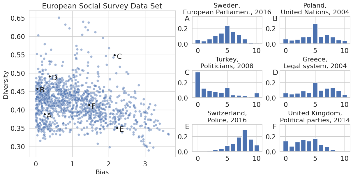
Within the attitude distributions of this data set, we mostly observe one central peak at 5 and one off-center peak.3 Sometimes also small peaks exist at the extremes 0 and 10. Similar to Example D in Figure 1. Many distributions have a low Bias looking close to normally distributed, like Example A. In most cases, if the Bias increases as in Example F or more subtle as in Example D, the distribution gets an off-center peak. Here, Example D has two additional off-center peaks. Example B can be seen as a more extreme case of this phenomenon. Due to two equally sized off-center peaks and one at the extreme, and an especially pronounced one at 0. Resulting in almost no Bias and a high level of Diversity. If the center peak is ignored or the distribution does not possess one, the overall distributions resemble a bell shape or a skewed bell shape. These shapes can have higher Bias and lower Diversity like example E or higher Diversity and higher Bias like example C.
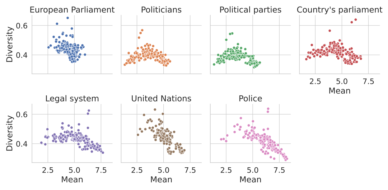
Figure 15 in the Appendix displays an overview of the mean and Diversity of each distribution of the data set to split with respect to the individual questions. In comparison, one can conclude, that the direction of trust is topic-dependent, e.g overall Europe the trust in police indicates a positive relationship of trust, in contrast to political parties or politicians, which are not being trusted. The only more diverse topic is trust in the legal system, which is mainly country-dependent.
The ESS dataset provides many different distributions which we will use to calibrate model parameters in the following. The large variety of distributions allows for assessing if the model can replicate this variety. The ESS dataset is provided in the reproduction material (European Social Survey ERIC (ESS ERIC) 2016). The disadvantage of the ESS is that we do not know if individuals change their attitude over time (let alone the social interaction of individuals which is an integral part of the agent-based model). Panel surveys have answers from the same individual for several years. Thus, they can provide a different type of information to compare empirical data and model output.
Political trust data in the Swiss Household Panel
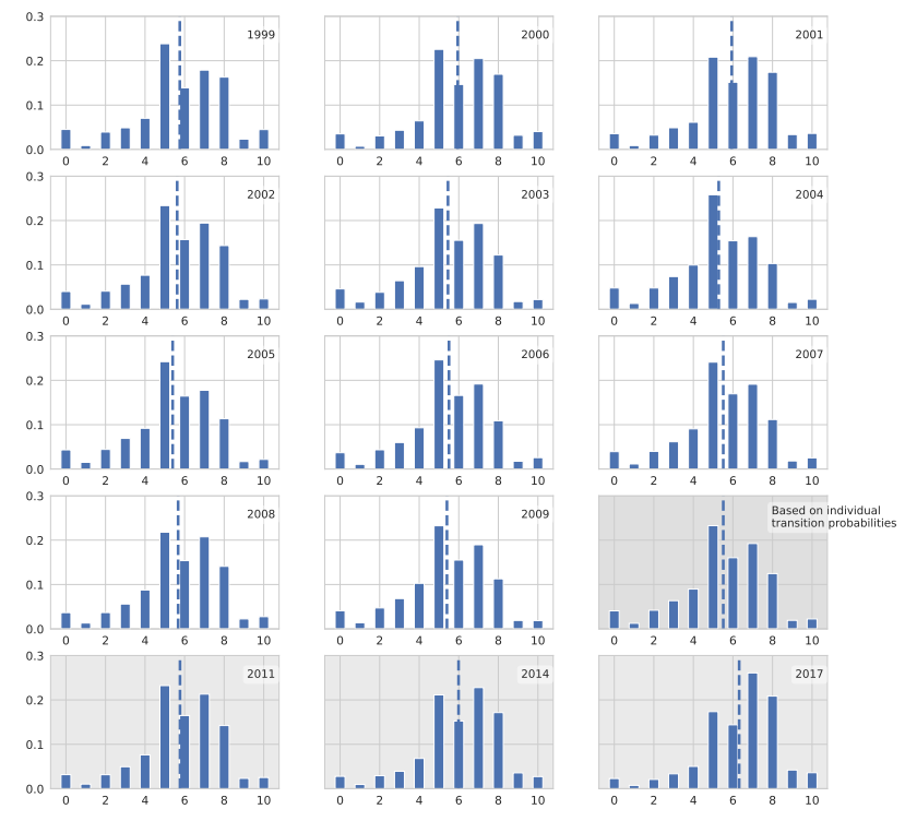
Within the Swiss Household Panel (SHP) we use the Trust in Government4 question which was conducted from 1999 to 2009 annually and in 2011, 2014 and 2017 again (Figure 2)(FORS 2023). During this first eleven year time period the overall fluctuations are minor and the mean is always between 5 and 6. In 2017 we can see a bigger increase in trust in attitude distribution. However, we neglect the last three rounds in further analysis to have equidistant time steps.
From the data from 1999 to 2009, we extract the annual transition probabilities with a total of 50008 recorded opinion shifts from 10627 individuals.
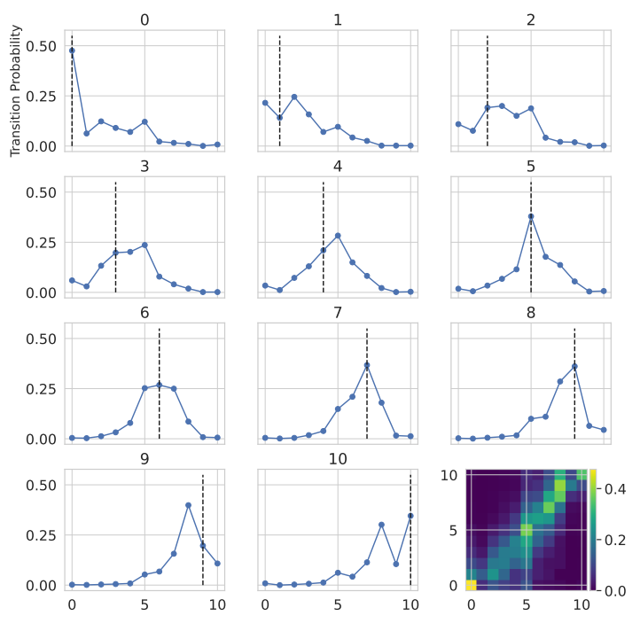
We use aggregated transition probabilities over all years. In the preliminary analysis, we did not find major variations in the transition probabilities in different years. With aggregated transition probabilities we interpret these transition probabilities as a long-term personality trait of individuals on an aggregated scale. Consequentially, a person with less trust in government (answer 2 to 4) is more likely to answer 5 in the next round.
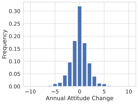
Independent from the transition probabilities the distribution of annual change is showing the distribution of attitude changes in a time frame of one year. Meaning, that if an individual has an attitude value of 3 and in the next year he or she changes to 5, the annual attitude change would be +2. For the empirical data, the distribution is displayed in Figure 4. Though the transition probabilities suggest a high degree of fluctuation on the micro level, this distribution shows that the majority of individuals do not change their attitude or only change in the range of \(\pm 1\).
The Opinion Dynamics Model
We use the model of continuous opinion dynamics presented by Lorenz et al. (2021). In the model, the opinions of \(N\) individuals are represented by real numbers. The opinions of individual \(i\) at time step \(t\) is \(a_i(t)\).5 The model assumes that initial and idiosyncratic opinions come from a normal distribution and the opinions are bounded by a maximal and a minimal opinion lying symmetrically around a "neutral" opinion which forms the natural midpoint of the scale.
Our goal is to calibrate and compare the model output to empirical attitude data on an eleven-point scale from zero to ten. To that end, we specify the minimal opinion as \(-0.5\), the maximal opinion as \(10.5\), and the neutral opinion as five. That way, we can easily transform every continuous opinion to a discrete version by standard rounding to the nearest integer between zero and ten. The model of Lorenz et al. (2021) uses \(\pm M\) as minimal and maximal opinions and zero as a midpoint. This makes the mathematical formulation easier. Here, we use an equivalent version with a shifted neutral point to make outcomes and parameters better comparable to the empirical data.
In the following, we outline the model. It has the following parameters which we will later use for calibration: The change strength \(\alpha\) and the degree of assimilation \(\rho\) which are parameters of the core opinion change function, the latitude of acceptance \(\lambda\) and the acceptance sharpness \(k\) which are parameters of the motivated cognition factor, the idiosyncrasy probability \(\theta\) which specifies the degree of idiosyncratic opinion formation, and \(\sigma\) the standard deviation of the normal distribution where initial and idiosyncratic opinions are randomly drawn from.
Opinion change through social interaction
Within the model, agents communicate with each other in one direction. That means a receiver receives a message \(m\) from a source which is another agent, the receiver evaluates the message while the source remains unaffected. This is called a passive communication paradigm. This can be seen as the basic building block of opinion change through social interaction. It is a typical experimental setup in psychological experiments and can also be seen as an important mode of modern communication where people read news, blog posts, or their social media feeds. Rarely these communications are influencing the source rather than the receiver.
The basic mode of opinion update is:
| \[\begin{aligned} a_i(t+1)&= a_i(t) + \Delta a \\ \Delta a_i &= f(a_i,a_j) \end{aligned}\] | \[(1)\] |
The specific form and parameters of the opinion change function in Lorenz et al. (2021) were inspired by Hunter et al. (1984) who collected formal representations of attitude change in mathematical psychology. The core opinion change function with a neutral opinion of zero (as in the original model of Lorenz et al. 2021) is:
| \[\begin{aligned} \Delta a_i &= \alpha(a_j-\rho a_i) \\ \end{aligned}\] | \[(2)\] |
Additional to this basic version of the opinion change we also include the mechanism of motivated cognition, which means that agents tend to ignore opinions that are far away from their own opinion. With the inclusion of the motivated cognition factor the opinion change function changes to:
| \[\Delta a = \underbrace{\frac{\lambda^k}{\lambda^k + |a_j-a_i|^k}}_{\text{motivated cognition}} \alpha(a_j-\rho a_i)\] | \[(3)\] |
Opinion change can bring the updated opinion above the maximal (or below the minimal) opinion (whenever \(\rho > 0\)). When this happens the opinion is set to the maximal (or minimal opinion) of 10.5 (respectively \(-0.5\)).
Timeline and idiosyncratic opinion change
A simulation run of the model starts with the initialization of \(N\) agents with initial opinions being random numbers from a normal distribution with mean five (the neutral opinion) and standard deviation \(\sigma\). The simulation then runs in discrete time steps while in each time step, all agents update their opinion in random order. The following Figure 5 is showing the histogram of probabilities for the initial opinions for each corresponding \(\sigma\). Due to our confinements, \(\sigma\) = 3 also produces maxima at the extremes. Additionally, the Diversity is added to the individual distribution to compare the initial conditions to the empirical distributions in Figure 1.6
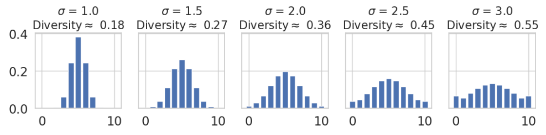
Our initial Diversity is evenly spread between 0.18 and 0.55, which is lower than the empirical Diversity from 0.3 to 0.65, but the range covers the majority of empirical Diversity.
Most opinion updates or through social interaction as specified above. However, opinion change can also happen idiosyncratically. The idiosyncrasy probability \(\theta\) defines how likely that is. When an agent is up for opinion change it is decided randomly with the idiosyncrasy probability if social interaction is skipped and instead the agents change its opinion back to its initial opinion \(a_i(0)\).
Lorenz et al. (2021) model idiosyncratic opinion change as the draw of a new random opinion in the same way as the initial opinion. The model we use here (change back to the initial opinion) is also mentioned there. In many situations, this change does not change the model behavior on the macroscopic level, however, it changes the trajectories of individual agents. This choice can also be motivated by Inglehart (1997) arguing that political trust is learned in early life. The initial opinion can be seen as the opinion when entering adulthood. Still, social influence can change their opinion but there remains a propensity to change back to that default opinion.7
Model behaviour
The model is able to reproduce certain shapes of opinion distributions, which are explained hereinafter. In the basic model without any idiosyncrasy, the model always creates a consensus with all agents having the same opinion. If \(\rho <1\), agents move (at least a bit) toward the sign of the messaging agent. This can result in all agents moving toward one of the extremes instead of forming a consensus in the center. The parameter \(\alpha\), change strength, decreases the time needed until consensus (extreme or central) is reached.
Idiosyncratic opinion formation through the rate \(\theta\) can counter assimilation as well as a drift to the extreme by constantly feeding in the distribution of initial opinions. Drift to the extreme and inflow of the initial distribution can be in balance, such that the distribution stabilizes with a certain bias and a peak between the center and one of the extremes. The direction of the bias is subject to randomness. The direction is decided randomly through the initial opinions as well as to a certain extent to the order of interactions in the first time steps. Figure 6 highlights the emergence of stabilized distributions in examples a-e with the corresponding initial opinion distribution (red hatched bars).
For example, if the degree of assimilation \(\rho\) is very high and the initial opinion spread \(\sigma\) is low, the motivated cognition influence is rather small. Resulting in all opinions concentrating in the center and converging to a central consensus with low diversity. In contrast, example b shows a lower degree of assimilation, which results in a higher degree of opinion shifts towards the extreme. Nevertheless, the motivated cognition and low strength \(\alpha\) in conjunction with the idiosyncratic opinion shifts are keeping the overall opinion distribution similar to the initial distribution but with a slightly increased diversity.
Example c shows how a peak drifted to one extreme. Notice, that the differences in parameters are subtle. The drift to the extreme is triggered by \(\rho = 0.7 < 1\), however, \(\rho\) is even lower in example b where no drift appeared. The higher \(\alpha\) in example c makes the drift faster and additionally the slightly lower idiosyncrasy probability \(\theta\) does not bring enough new more central opinions. Example d then shows an example with a small bias with an off-center but not extreme peak (d).
Motivated cognition with the latitude and sharpness parameters \(\lambda\) and \(k\) reduces the strength of interaction between agents if their opinion difference increases. However, the essentially unimodal phenomenology of examples a-d can in a similar form also be observed without motivated cognition in the model (see Lorenz et al. 2021). However, motivated cognition can change the exact shape of the unimodal distributions and this can help to come closer to the replication of empirical distributions as we will see later.
Motivated cognition is however essential to create bipolarization and fragmented multimodal opinion distributions. Example e in Figure 6 shows two groups separating and moving to opposite sides. This happens concurrently towards stable bipolarization, but it can also happen alternately in an ever-continuing oscillation through idiosyncrasy (f). The distribution in example f never stabilizes and therefore, such parameter settings are not included in the simulation data set which we produced.
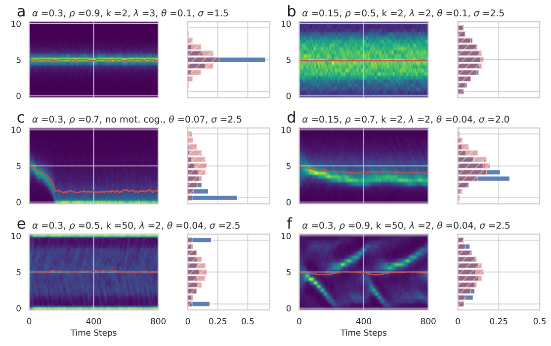
Comparing the outcomes of the model to the empirical distributions in Figure 1 qualitatively certain structural similarities can be detected. For example, example c shares a high degree of extremity with the distribution of trust in the politicians in Turkey (C).
Methods
In the following, we explain how we calibrate the parameters of the model such that empirical data is best matched by the model outcome. The idea is, for example, to match the empirical distributions, as for example shown in Figures 1 and 2, with a parameter configuration of a simulation such that the emerging stabilized distribution, as for example shown in Figure 6 is similar.
To that end, we specified parameter values for a parameter sweep to produce a simulation data set. Table 2 shows all parameter values. We ran ten simulations run for each parameter combination. For \(\alpha\), \(\rho\), \(\theta\), and \(\sigma\) we have \(5 \times 5 \times 3 \times 5\) combinations which we use for simulations without motivated cognition and additionally also with motivated cognition using \(4 \times 3\) combinations for \(\lambda\) and \(k\). In total there are 4,875 parameter combinations and 48,750 simulation runs.
For each simulation run, we use 800 agents and a minimum of 1000 time steps. In each time step, every agent interacts either once with respect to the opinion of another random agent or idiosyncratically. If the opinion distribution of the simulation is only fluctuating and no more major changes occur, we record the outcome. Otherwise, we continue running the simulation until a maximum of 1500 time steps. In the following, we describe the stopping criterion in detail and how we compute transition probabilities, the stabilized (stationary) distribution, and the distribution of individual changes from the simulation data. The computation of transition probabilities and the distribution of individual change can be done for different time step counts (TSC), which means how many time steps we let pass to measure the individual change of opinion and its distance. This delivers another optimization parameter with respect to the empirical SHP data. Optimizing the TSC would specify how many time steps in the simulation match the yearly time interval of the SHP best. (Details in the following subsections.)
In the following, we describe the goodness-of-fit measures we use to compare simulated and empirical data. The goodness-of-fit measures are then used to select the best-fitting parameter constellation for each country-topic-year combination of the ESS data set and for the SHP panel data.
In this way we produce three data sets:
- The simulation data which includes 41163 observations, one for each of the 10 simulations for each of the 4,875 parameter constellations specified in Table 2 for which simulations converge to stabilized opinion distributions. In addition to the parameters, each observation contains
- the stabilized opinion distribution (fractions on the eleven-point scale),
- the transition matrix (for one time step and the transition matrix that utilizes bigger time steps and has the best fit), and
- the change distribution (based on these bigger time steps).
- The empirical data set of the ESS with the best fitting simulation parameters for the opinion distribution.
- The empirical data set of the SHP with the best fitting simulation parameters for the opinion distribution.
The data sets are available at the open science foundation (osf) here: https://osf.io/fsbda/?view_only=5e76c7f45dbf480b9672138fae1186b4.
| Parameter | Values | Description |
|---|---|---|
| \(\alpha\) | 0.1, 0.15, 0.2, 0.25, 0.3 | Change Strength |
| \(\rho\) | 0.1, 0.3, 0.5, 0.7, 0.9 | Degree of Assimilation |
| \(\theta\) | 0.04, 0.07, 0.1 | Idiosyncrasy |
| \(\sigma\) | 1, 1.5, 2, 2.5, 3 | Initial Opinion Spread |
| if motivated cognition module is added: | ||
| \(\lambda\) | 1, 2, 3, 4 | Latitude of Acceptance |
| \(k\) | 2, 10, 50 | Acceptance Sharpness |
| *10 repetitions for each parameter configuration |
Stopping criterion
Because we are using agent-based modeling with the inclusion of idiosyncratic opinion shifts (noise), these models possess a -casually speaking- spin-up-time after which the dynamic stabilizes. After this point in time, only minor fluctuations occur. Henceforth, we define the moment in time when the simulation stabilizes macroscopically as steady state and, additionally, based on the steady state, a stopping criterion for the simulation run. For evaluating if the dynamic stabilized, each time step a distribution with 30 equally sized bins in the range of the opinions is calculated. As a measure, if the dynamic stabilized, the euclidean distance from the initial distribution \(ED=\sqrt{\sum_i (p_i(t) - P_i)^2}\) is calculated for each time step. With \(P_i\) being the attitude distribution at \(p_i(t=0)\) (initial distribution) and \(i\) indicating the bin of the calculated distribution. To conclude if the overall distribution remains stable (steady state is reached) a linear fit over the last 100 time steps is performed and the absolute slope has to be \(|m|\leq 0.001\) otherwise the model will continue running. Concluding, in the last 100 time steps the dynamic already stabilized.
We continue the simulation until it meets the criterion or a maximum number of 1500 time steps is reached. If a simulation run never suffices this criterion because e.g. features oscillating dynamics as in example f in Figure 6, its data is excluded for further evaluation.
Additionally, we use the \(ED\) measure to quantify the time steps in which the model already reached its steady state to enhance further evaluations. Therefore, we keep the last 50 time steps and the corresponding measure as the distance from the initial distribution. Instead of using the 50 time steps before, we shift the measures 10 time steps in the past. Hence, we test if the distributions from the 110th (counting backward from the last time) until the 60th time steps and the 50th until the last time step still suffice the previous criterion. We shift the measure until the simulation run does not satisfy the criterion anymore and calculate the time steps in the steady state accordingly.
Stationary distribution
For assessing our resulting distribution to the according set of parameters, we use the agents’ transition probabilities after the previously calculated steady state is reached. For calculating the transition probabilities from a continuous scale, the agents’ attitudes are rounded to the next integer. The transition probabilities \(T(i=x,j=y)(t)\) are representing the probability of agent \(i\) with opinion \(x\) at \(t= t\) to switch to opinion \(y\) at \(t'= t+ 1\) in the next time step. We approximate the transition probabilities as constant over time, \(T(t) = T\), henceforth, this means that the dynamic is approximated as a Markov chain (referring to transition probabilities).
Following the argument of transition probabilities being a long-term personality trait, allows us to calculate the stationary distribution from the transition matrix. From a simulation perspective; the stationary distribution is the distribution that emerges from every possible distribution if the transition probability matrix is multiplied by it \(n\) times with \(n\rightarrow \infty\). Or in mathematical terms, the stationary distribution is the normalized first eigenvector of the transition probability matrix. Note, in our case, the stationary distribution is very similar to the distribution that would emerge from a simulation with \(t\rightarrow \infty\) and then averaged over all time steps.
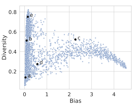
On the foundation of the stationary distribution, we calculate the bias and diversity and the average of these measures for each parameter configuration. As mentioned the bias of each simulation run is determined by a degree of randomness, therefore bias is defined as the absolute deviation from the center of the scale. Thus, high bias characterizes societies of high trust as well as high distrust. This results in Figure 7 including references to the previous examples in Figure 6.
In Figure 2 (last column 4th row), labeled Based on individual transition probabilities the stationary distribution based on the empirical transition probabilities of the SHP is displayed.
Goodness-of-Fit
For the evaluation of the goodness-of-fit, we split this into 2 subsections. First, the evaluation of simulation data to opinion landscapes (macro) and, second, the quantitative comparison of agents’ opinion transitions to ones of individuals in panel data (micro).
Comparing to macro data - Defining Goodness-of-Fit
In the first step, the model results are compared to the ESS dataset and the aggregated opinion landscapes in a country in one round. To quantify the goodness-of-fit we use the \(R^2\) value defined as follows:
| \[R^2 = 1 - \frac{\sum_{i=0}^{10} (q_i - x_i)^2}{\sum_i^{10} (q_i - H_0)^2}\] | \[(4)\] |
The distribution for comparison \(Q = Q(q_i)\) is the stationary distribution for one set of parameters and \(X = X(x_i)\) is one empirical attitude distribution. \(H_0\) is our null hypothesis with a binomial distribution of \(p=0.5\).8 Concluding our \(R^2\) is explaining the variance to a binomial process.
Due to the degree of randomness, we repeat each simulation for a set of parameters 10 times. If the majority of simulations do not reach a steady state the parameter set is neglected otherwise the mean of \(R^2\) for one set of parameters is evaluated as its goodness-of-fit.
We evaluate the best for all distribution within the ESS political trust data set. In fact, after a big parameter sweep, we find the parameter set which resembles each attitude distribution within the ESS in the best way possible (has the largest \(R^2\)). For each simulation run, we consider both directions of bias. Meaning we compare each empirical attitude distribution to every simulated distribution and the equivalent mirrored one.
Comparing to micro data - Defining Goodness-of-Fit
The introduction of panel data enables the evaluations of goodness-of-fit in a much greater variety. In our case, we utilize transition probabilities and the distribution of annual change to compare agents to individuals. Therefore we define a measure of goodness-of-fit for the first by comparing the \(11\times11\) transition probability matrices.
Also considering that a time step in the simulations is not equivalent to a time step in the empirical data, we deviate from the previous definition of the transition probability and calculate the transition probabilities from 1 up to 30 time steps as a possible equivalent annual time step (TSC).
However, the corresponding increase in time steps for the transition probabilities is changing the previously defined stationary distribution because our transition probabilities (and approximated Markov chain) are not time-homogeneous. Depending on the size of \(TSC\) these differences can become larger but are not significant in our case and neglected in the following.
All things considered, evaluating the goodness-of-fit of two transition probabilities is defined with the Euclidean distance9 or a not standardized mean squared error:
| \[D_{micro} =\sqrt{ \sum_j^{11} \sum_i^{11} (Y_{ij} - T_{ij})^2}\] | \[(5)\] |
Lastly, the distributions of annual change are compared. This measure comes in handy because of its lower dimensionality and its partial independence from transition probabilities, especially if only shorter time frames are investigated. To create this distribution from simulated data for comparison the previously optimized time step count (TSC) is used to mimic one year time frames. Later, the empirical and simulated distributions of annual change are compared qualitatively.
Results
In the next section, the empirical attitude distributions from the ESS data set are calibrated for answering research question 1 and 2. Followed by a calibration of the annual attitude distributions of the SHP and a concluding comparison between the individual and simulated data.
Comparison to ESS data set
All resulting stationary distributions are compared to all attitude distributions in the ESS and the corresponding \(R^2\) values are calculated. For each empirical attitude distribution, the best-fitting set of parameters was saved. Figure 8 displays all \(R^2\) values in the bias-diversity plane and shows the resulting fits for our exemplary attitude distributions.
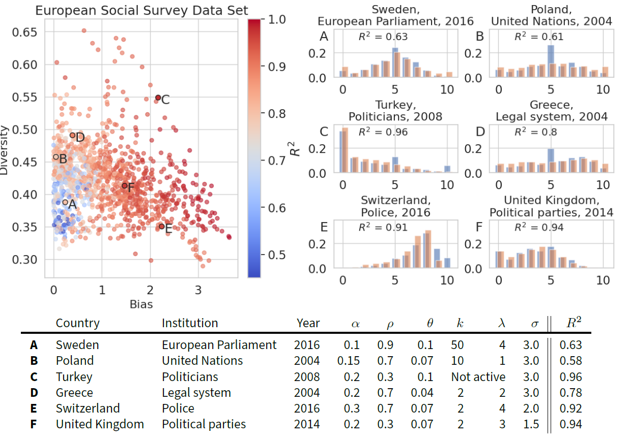
From the bias-diversity plane, we can conclude that higher bias is resulting in higher \(R^2\). There are two reasons for that, first, higher bias is in most cases an indicator of less bipolarization. Empirically speaking, a country’s population agrees on the degree of trust and the overall distribution has a single and more pronounced off-center peak. This kind of distribution is fitted extremely well with our model. Secondly, the higher \(R^2\) values are a byproduct of bigger differences to our null hypothesis in the definition of \(R^2\). Subsequently, more extreme distributions are resulting higher values in the denominator in the definition, henceforth, higher \(R^2\). Distribution C, E, and F are prime examples of this effect with \(R^2 >\) 0.9. In C and F, the only shortcomings of our model are at the extremes 0 and 10 and at the center of the distribution. In trust in the police in Switzerland (E) the fit mostly lacks the overall sharpness of the peak. In contrast, the trust in the European parliament in Sweden (A) distribution resembles a normal distribution like our null hypothesis with a higher central peak, resulting in a lower \(R^2\) nevertheless being fitted extremely well. The trust in the United Nations in Poland (B) is similar in this regard, but with a very significant central peak that cannot be fitted. Trust in the legal system in Greece (D) is showing a multimodal structure with 2 off-center peaks, at 3 and 7, which the model is also unable to fit, contributing to a lower \(R^2\). Concluding from our six exemplary fits, the simulated distributions match the overall shape in most cases, except for the center and extremes or structures with two equally sized off-center peaks.
Comparing the parameter, the trust in the European parliament in Sweden in 2016 (A) shows a very uniform distribution with low strength \(\alpha\), high assimilation \(\rho\) and idiosyncrasy \(\theta\) of 0.1. The initial opinion spread \(\sigma\) is also very high. This parameter configuration has a similar dynamic to example b in Figure 6 resulting in a centered normal distribution. Compared to trust in politicians in Turkey (C), the strength parameter is doubled and the degree of assimilation \(\rho\) is significantly lower at 0.3. Additionally, the motivated cognition module is not active, resulting in agents assimilating more to extreme opinion values (example c in Figure 6). Examples D, E, and F, in this regard, have a very shallow bound considering \(k = 2\) and lower idiosyncrasy similar to the dynamic in example d creating a single off-center peak. Comparing example F to C with the same \(\alpha\) and \(\rho\), F has a lower Bias due to the motivated cognition, though having a lower idiosyncrasy (which would typically increase the overall bias). The fits in D and E are similar in shape, with a smaller latitude of acceptance \(\lambda\) in D, which is decreasing the Bias and increasing the Diversity. Additionally, the initial opinion spread \(\sigma\) is higher for Example D, increasing the diversity furthermore.
Additionally in the Appendix, Figure 16 displays the distributions for each individual parameter of the data set fitted to the ESS.
Knowing that most fits are utilizing a small sharpness (\(k=2\)) and high latitude of acceptance (\(\lambda\)=4), meaning that the motivated cognition does not have a big impact on most of the attitude changes. Therefore we create a subset of the simulation data, only consisting of simulation runs without the motivated cognition active and fit it to the ESS data. Enabling us to compare the outcomes of the model with motivated cognition to ones without. In Figure 9 a box plot of the best fit for the complete data set and a subset is displayed and split into the institutions of political trust. First, fits for all institutions perform on a similar level with a median \(R^2>0.8\), except for trust in the European parliament. Trust in the United Nations, the police, and the legal system are the topics with fewer outliers towards \(R^2<0.6\) but also fewer distributions towards \(R^2 \approx 0.9\). Additionally, the exclusion of the motivated cognition module shows a significant decrease in performance for the model for all institutions, observing a much higher spread of \(R^2\) and a lower median. Concluding that this module is an integral part of fitting empirical distributions about institutional trust.
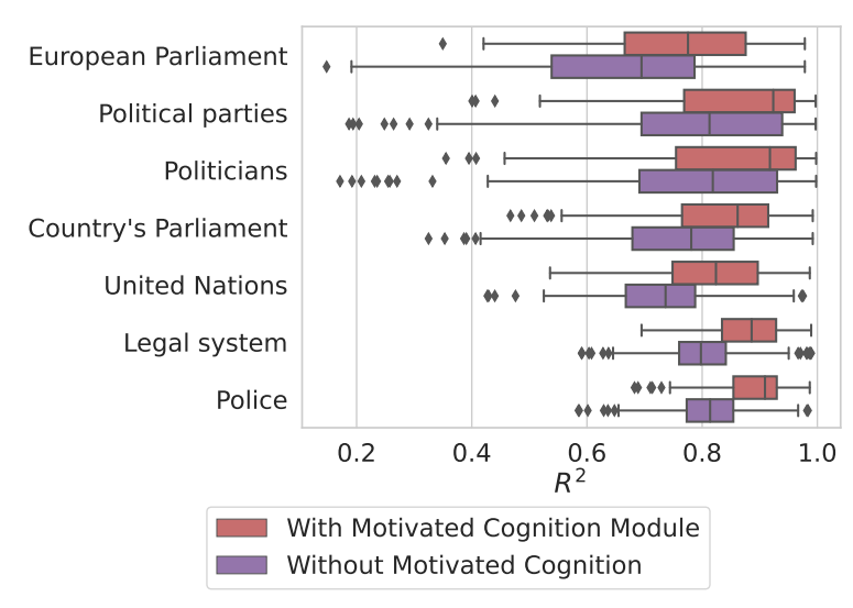
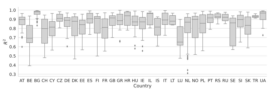
Lastly, we take a look at a country-wise distribution of \(R^2\) (ref. Figure 10). Here we see a higher variance between the countries, compared to the variance between the questions in Figure 9. Nevertheless, the median never falls below 0.6 for any country and with the most outliers towards low \(R^2\) for the Netherlands.
To conclude our Research Question 1, we are in most cases able to reproduce the attitude distributions on the question of trust in institutions in the ESS with a high level of accuracy with a single opinion dynamics model. Furthermore, we can conclude, that the inclusion of the motivated cognition module is one of the key features to enable this level of accuracy.
Comparison to SHP data set
First, we are remaining on the aggregated level and compare each year within the dataset to the model results on the macro level. After, we take the evaluation a step further and use individual data to facilitate the results. When comparing empirical individual data to our simulation we also have to keep in mind that we approximate the empirical data as representative. The approximation is an effect of data cleaning, lack of weighting, and reducing the dataset by only using opinion transitions that happen in a time span of one year.
Comparing Model to macro data
After concluding that the empirical aggregated opinion distribution of the ESS can be fit by our model, hereinafter the annual data from the SHP (Figure 2) is fitted accordingly. The results are displayed in Figure 11.
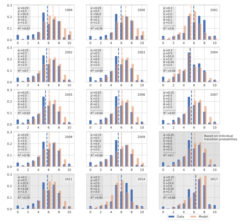
As shown, all years can be reproduced on the aggregated level with a \(R^2\) between 0.56 and 0.88. The dashed lines show the arithmetic mean for the simulated and empirical data, which have the largest deviation in the beginning, in 1999 and 2000. The majority of the parameter values needed to fit each year individually are \(\alpha = 0.25\), combined with \(\rho = 0.5\), \(\sigma = 2\), \(\theta = 0.01\), \(k = 2\), and \(\lambda = 4\). Additionally, this configuration is also used to fit the stationary distribution based on the individual transition probabilities. This is due to the overall similarities of the attitude distributions and high fluctuations on the micro but not on the macro level. This particular parameter configuration is causing that typical off-center consensus like described before (ref. example d in Figure 6).
Nevertheless, overall we can conclude that the attitude distribution about trust in the government in Switzerland like most of the distribution in the ESS can be fitted with our model, except for a systematical shortcoming at the center and extremes.
Comparing Model to micro data
By utilizing the potential of panel data, in the following, the transition probabilities of agents are compared to individuals.
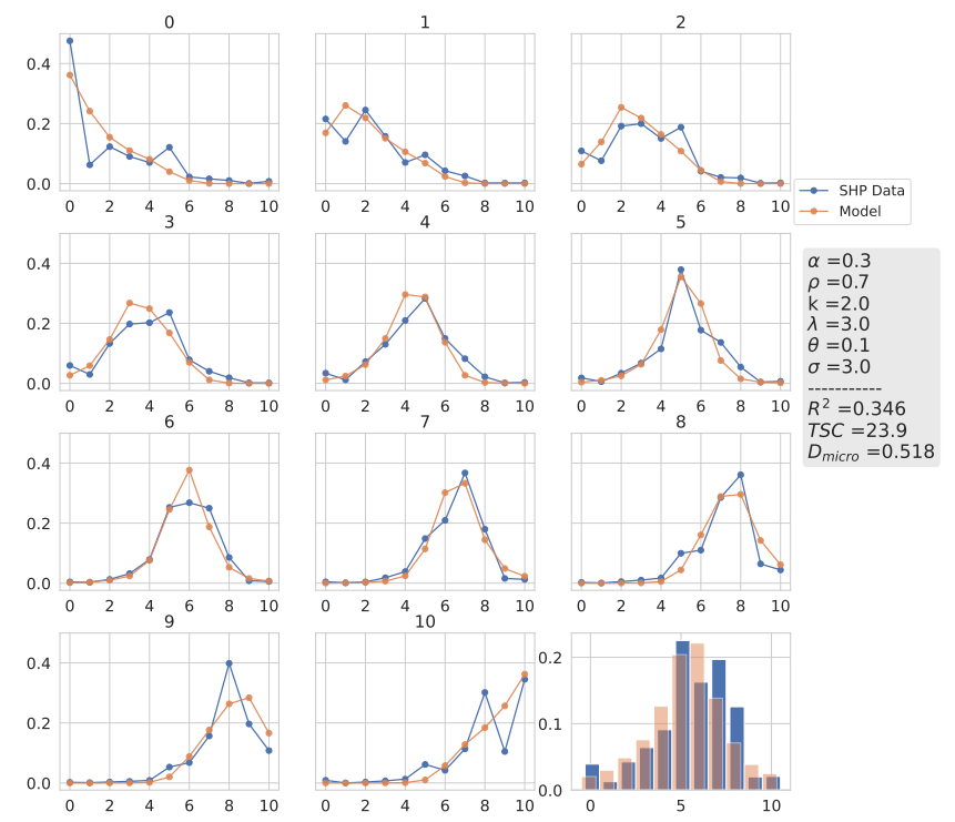
First, the result with the parameter set which reproduces the best microscopical fit or highest \(R^2\) is displayed in 12 and, at first glance, the simulated data matches the empirical data also on the individual level. The average time step count (\(TSC\)) to achieve a \(D_{micro} =\) 0.517 is 24.8. Additionally, the stationary distribution based on the displayed transition probabilities is calculated and shown in the bottom right corner. As discussed previously and if the distribution is compared to the one in 11, it is apparent that the increase in TSC does not have a major influence on the stationary distribution.
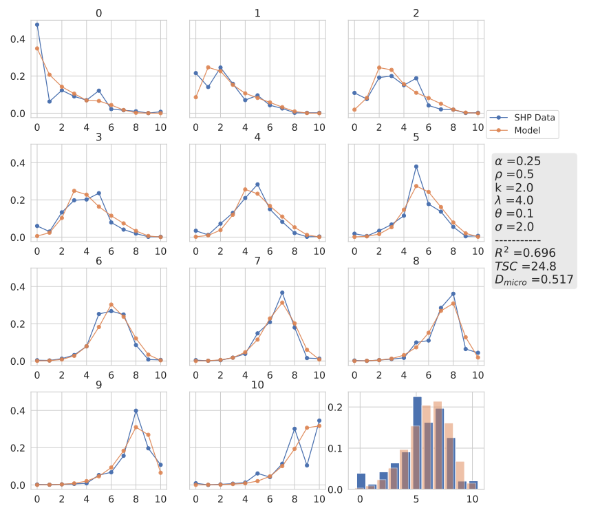
Looking closely at the individual graphs, we can observe minor shortcomings, like at the extremes 0 and 10. Here, the model is reproducing the highest peak quantitatively but lacks the ability to reproduce the probability dip at 9 and 1 respectively. Additionally, the overall shape of the simulated data resembles more an exponential decay than the shape of the empirical data. Concluding, the model is missing a mechanism for individuals with extreme opinions. For the other opinion transitions, the simulated probability to move to the center is always below the empirical one, pointing to another missing mechanism. Otherwise, when comparing the highest probabilities within each graph, their position matches or deviates by only \(\pm 1\) except for opinion 3.
Secondly, we want to compare the result to the transition probabilities with the smallest \(D_{micro}\). But the result based on our \(R^2\) also produces the smallest \(D_{micro}\). Therefore as a comparison, the result with the second smallest \(D_{micro} = 0.518\) (compared to \(D_{micro} = 0.517\)) is chosen. Here, the difference in \(D_{micro}\) is negligible due to a degree of randomness in the simulations and, consequently, reduced accuracy of the measure. Interestingly, the \(R^2\) values differ significantly (\(R^2 = 0.346\) compared to \(R^2 = 0.698\)), hence we look for significant differences in the results, as well as in the used parameters. For a cohesive comparison, the parameter values and goodness-of-fit measures are also displayed in Table 3.
| \(\alpha\) | \(\rho\) | \(\theta\) | \(\sigma\) | \(\lambda\) | \(k\) | \(R^2\) | \(D_{micro}\) | \(TSC\) | |
|---|---|---|---|---|---|---|---|---|---|
| Best Fit | 0.25 | 0.5 | 0.1 | 2 | 4 | 2 | 0.698 | 0.518 | 24.8 |
| Example B | 0.3 | 0.7 | 0.1 | 3 | 3 | 2 | 0.346 | 0.517 | 23.9 |
Both simulated transition probabilities do not show significant differences and have similar shortcomings. In some cases, our second example is a better fit, like for opinion 5 but is slightly worse for opinion 8 or 9. Summarizing, our second example fits the maxima in the transition probabilities better and the overall individual shapes of the transition probabilities worse.
Although the \(R^2\) values differ significantly, the parameters show only slight differences. The strength parameter \(\alpha\) varies between 0.25 and 0.3, and the degree of assimilation between 0.5 and 0.7. Concluding, in this case, if the strength increases, the overall degree of assimilation also has to increase to keep similar individual transition probabilities. All in all, the individual probabilities have a low spread and the majority of opinion shifts occur in the range of \(\pm 2\) from the starting opinion. Additionally, the initial opinion spread \(\sigma\) increased in combination with \(\alpha\) and \(\rho\). The idiosyncrasy is the same for both examples, \(\theta=0.1\), and the motivated cognition also only differs slightly. The latitude of acceptance has a bound at 3 or 4 with the same low sharpness of \(k = 2\).
Lastly, we compare both distributions of annual opinion change against the empirical one in Figure 14.
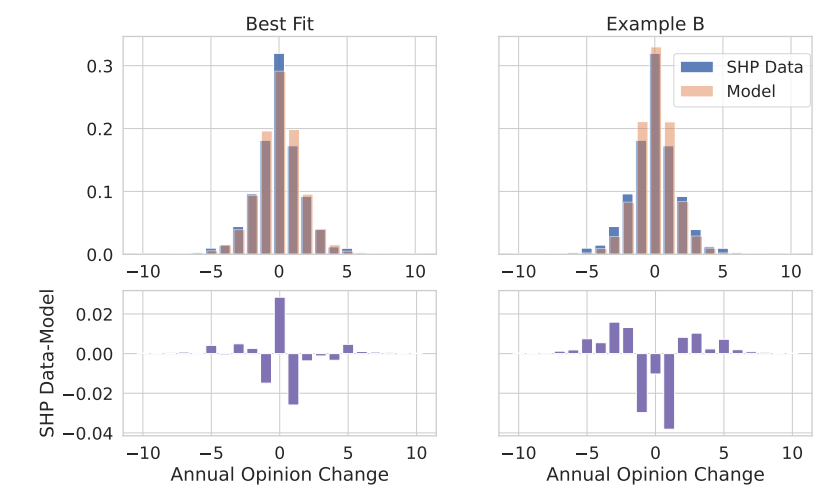
Both distributions fit the empirical one well, but our best \(R^2\) and \(D_{micro}\) fit is visibly better here. This can be manifested by the plots below, displaying the differences between the simulated and empirical distributions whereby the Best Fit has less deviation, especially above annual opinion changes of \(\pm 2\).
Finally, to answer our second research question, the model is able to reproduce the transition probabilities of individual opinion change as observed in the SHP. Additionally, we also observe a high accuracy in the distribution of annual opinion change and overall, the parameters match the outcome of the analysis in the ESS. Nevertheless, similar shortcomings when calibrated to the empirical data are present on the aggregated and individual level.
Discussion & Conclusion
The real-world application of opinion dynamics models has been discussed in literature intensively, nevertheless, the comparisons of model outcomes and empirical attitude distributions on the macro and micro level are lacking. In the first part, we showed that the questions about political trust in the ESS can be replicated on the macro level by the model framework of Lorenz et al. (2021) using psychologically motivated attitude change functions from Hunter et al. (1984). We find that the goodness-of-fit does not vary systematically with the different trust institutions or the different countries.
The inclusion of the theoretical assumption of motivated cognition when assessing others’ opinions, showed a substantial increase in the goodness-of-fit in performance when fitting simulated attitude distributions to empirical ones. In the model, the motivated cognition module is essential to produce the phenomena of bipolarization and fragmented multimodal distributions. Both of these appear very rarely in distributions concerning trust questions in the ESS.10 However, it improves the fit also in situations without fragmentation.
The most common parameters for motivated cognition in our parameter sweep are the largest latitude of \(\lambda = 4\) and a low sharpness of \(k=2\). Lorenz et al. (2021) showed that these parameters are not prone to produce fragmented distributions but they can produce bipolarization when the degree of assimilation \(\rho\) drops towards zero. Under the assumption of these parameters, many societies may be prone to bipolarization on political trust when attitude change would becomes less assimilative and more moving in the direction of the attitude of others (lower \(\rho\)).
In the ESS dataset, the majority of best fits show a degree of assimilation of \(\rho =0.5\) or 0.7. The \(\alpha\) is typically between 0.15 and 0.3. The level of idiosyncratic opinion shifts is high for most of the ESS fits and the SHP fits of individual data. \(\theta = 0.1\) means that every time step with a probability of 10% an agent moves back to its initial opinion. Combined with dynamics towards one of the extremes, this results in a high proportion of large opinion shifts that are triggered by idiosyncrasy. In these parameter settings, the degree of assimilation is enough to create a joint bell shape instead of bipolarization. This shape then jointly moves either towards low or high trust being "stopped" by attrition through idiosyncratic opinion formation. Once the direction has been decided by random chance the bias stabilizes at a certain level of extremeness. However, the parameters \(\rho\), \(\alpha\), and \(\theta\) are related with respect to the level of the evolving bias: For example, lower \(\rho\) may be compensated by larger \(\alpha\) and lower \(\theta\) to lead to a similar level of bias. Therefore, drawing conclusions about the strength and degree of assimilation in the real-world interactions should be done cautiously.
We showed that panel data provide an opportunity to compare individual opinion changes in the data with individual opinion changes in the model. We demonstrate that calibrating parameters based on empirical transition matrices yields fit of similar quality than fitting with respect to the attitude distribution. While fitting we also needed to optimize how many simulation time steps have to be aggregated to produce best the empirically observed annual transitions. The best-fitting time step count is 24. That means, the model fits best to empirical data in the SHP when we assume that individuals tend to reconsider their opinions in social interaction on average 24 times a year, which we consider a reasonable value. Note, that a reconsideration of an attitude need not trigger a drastic change in the model.
As discussed, the direction of the evolving bias in a simulation run of the model is determined through randomness in the initial conditions and first interactions. That means a high trust as well as a low trust society is equally likely. For our evaluation, we used scale mirroring on the simulated data to account for both scenarios. That means the direction of the bias of our simulations is dependent on the compared empirical distribution. Combining both arguments concludes that trust in institutions is formed by early events and remains in this direction of bias. After the emergence of trust or distrust, it becomes very difficult to change. Even though there is an exchange of opinions, these distributions remain stable. These results are both coherent with the life-long learning model of Schoon & Cheng (2011) and the observations of Inglehart (1997) who argue that change of societal trust to distrust or vice versa, multiple generations are needed.
A limitation of the model is the lack of ability to fit the amount of extremist and central opinions, especially on the micro level. Here, extremist individuals are having a very high probability to remain extreme, including a very low probability of changing their opinion only one step on the attitude scale. One point of discussion, here, is that the empirical attitude distribution used for comparison completely ignores scale construction theory and the findings that the midpoint of the scale is often misused as a non-answer. We see in the data that people around the midpoint are changing their opinion less and/or less frequently. Nevertheless, we neglect this feature in our model because of the degree of complexity and uncertainty in the degree of non-answer and real neutrality in individuals. The 3 answers, 0,5, and 10 can be also interpreted in a different way and studies showed that answer 5 may also be substituted for "don’t know" or undecided answer (Nadler et al. 2015).
The decision to use only stationary distributions in our evaluations stems from the empirical reality, that in recent years opinion distributions have been empirically mostly stable over time, especially concerning politicized issues. In the literature, trends toward radicalization or bipolarization are discussed but they are rarely observed in the responses in European surveys. From that perspective, we consider the following assumption most plausible for our study: Empirical opinion distributions are stationary macroscopic distributions in which individuals continue to change their opinions.
Is this now an empirical validation of the model of Lorenz et al. (2021)? The answer to this question is a bit beyond the scope of the paper and also beyond what can be achieved with this type of data because it does not include information about the communication of individuals. What we did is the following: We took a model which was, in a sense, validated based on psychological theory and explored its generative capacity for macroscopic regularities by calibrating its parameters with respect to a goodness-of-fit measure (\(R^2\)). These goodness-of-fit measures can be seen as a measure for the validity of the claim that the model (under the calibrated parameters) is a candidate to explain the observed macroscopic patterns.
Utilizing 11-point scales in our work is also in line with the discussion of psychometric scales. Leung (2011) compared Likert scales by changing the number of response categories which did not affect (re-scaled) means and standard deviations. He also concludes that 11-point scales increase sensitivity and are recommended as self-reporting measurement scales. Additionally, Gestefeld et al. (2022) also showed in an exploratory analysis of 10 and 11-point scales, except for the decrease in sensitivity, no significant differences. Recently, Carpentras & Quayle (2023) analyzed psychometric distortion and by comparing 5 questions concerning trust in science, they concluded that political opinions are non-linear, which contradicts previous findings and should be considered in the future. However, we find it plausible to assume for our study that individuals can use the 11-point scale for interpersonal communication of trust on the same yardstick. At least, these are scales labeled only at their extreme points.
Our analysis is similar to Duggins (2017) who also compared empirical and simulated opinion distributions and achieved a high degree of similarity with his model. His model is also based on similar properties in regard to opinion change, like strength of interaction and latitude of acceptance (bounded confidence) but with a spatial component. Further on, our approach focuses on exploring parameter values and their influence on emergent opinion distributions. Additionally, our study developed a different framework of how to quantify the similarity between these distributions when noise is present including the evaluation of individual-level data.
For further research, one could always include additional modules of Hunter et al. (1984) and compare their impact on the results. In Lorenz et al. (2021) the module of polarity was also introduced as one of many. Further on, the combination of multiple modules can be investigated with the negative side effect of reduced understanding of the model and its dynamics. Because the degree of impact of each specific module becomes unclear. Additionally, in an exploratory analysis, we found no significant influence of heterogeneous parameter distributions within the agents on the outcome of the model. Nevertheless, for further exploration and a higher degree of realism due to differences in individuals, this feature could be included and analyzed in detail. Compared to measuring e.g. speed of particles, the measuring of attitudes is highly subjective and individual. Scales can also be interpreted differently by each participant for example over one’s lifetime or be dependent on someone’s life circumstances, experiences, or simply the well-being on the day of the interview. Therefore surveys, especially using longitudinal data, have a high level of inaccuracy when analyzed on the individual level.
With the basic calibration, this model allows the integration of more modules for further improvements of the fit. On the other hand, like in epidemiology, we also could observe e.g. the impact of variation in the model or the topology. These results then can foster our understanding of the emergence of polarization or other social phenomena. These variations are exceeding the capacity of this research but could be realized in the future.
Funding
The authors benefited from a grant by Deutsche Forschungsgemeinschaft (DFG – German Research Foundation) for the project “ToRealSim - Towards realistic models of social influence” to the fourth author - 396901899.Appendix
Distributions of ESS data
As addition the the Diversity-Bias plane the Figure 15 displays the a Mean-Diversity plane split into each institution. Similarities between topics within these two measures is indisputable, resulting in similar distribution of \(R^2\) when fitted, ref. Figure 9.
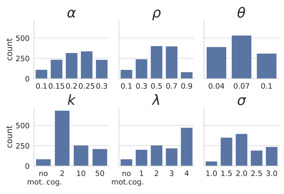
Parameter distribution of all ESS fits
The following plot displays the distribution of parameters to fit the ESS data set. Showing that our configuration of parameter values and limits were suited to fit the ESS data set because the distributions show no significant accumulation, especially at the limits. For an overall better fit, the steps could be decreased and \(\lambda\) be increased slightly in combination with an increase in number of agents \(n\).
Motivated cognition - \(\lambda\) and \(k\)
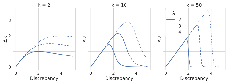
The module of motivated cognition is based on social judgment theory (Hunter et al. 1984 Chapter 4). One of the first hypotheses by Hovland et al. (1957) proposed: If someone receives a message with a large discrepancy the influence becomes repulsive, aka negative influence (or ‘boomerang’). They did not believe in this theory and proposed the theory of motivated cognition.
The initial theory lacks an acceptance sharpness \(k\) which was later included by Lorenz et al. (2021). The following Figure 17 displays the relation of \(\lambda\) and \(k\) and their influence on the opinion change function \(\Delta a\) depending on the discrepancy between the incoming message and the agent’s opinion. With \(k \rightarrow \infty\) the motivated cognition approaches the bounded confidence model, however, \(k = 50\) already reveals a very sharp bound.
Notes
Lorenz et al. (2021) speak about attitudes which we use as an equivalent of opinion in this paper. We use opinion in the modeling context because opinion dynamics is an established notion in agent-based modeling. We use attitude with respect to empirical data.↩︎
Another option would have been the Left-Right self-placement, but these distributions are more complex often showing a Pentamodal structure (see Gestefeld et al. 2022).↩︎
A peak is a bar in the distribution in which neighboring bars are (both) smaller.↩︎
Unfortunately, there are no direct equivalent political trust questions in SHP and ESS.↩︎
The letter \(a\) stands for "attitude" and is used for consistency with Lorenz et al. (2021).↩︎
For converting the model parameter \(\sigma\) to Diversity; Diversity\(=\sigma / 5.5\).↩︎
This mechanic can also be seen as a variation of the "anchorage" introduced by Friedkin & Johnsen (1990).↩︎
Our null hypothesis results from 10 Bernoulli experiments with \(p=0.5\). Or visually speaking, a Galton board with \(n = 10\) steps results in 11 possible bins, because all beads in the Galton board start at 5, equivalent to all individuals starting with neutral opinions, or as equation \(P(x)= 2^{-10}\binom{10}{x}\).↩︎
in this case also called↩︎
However, ESS attitude distributions show aspects of bipolarization for questions about European Integration in some countries (e.g. Serbia). Fragmented distributions with up to five modes appear for left-right self-positions and other questions as shown by Gestefeld et al. (2022). The calibration of the model to distributions of this kind is beyond the scope of this study.↩︎
References
AXELROD, R. (1997). The dissemination of culture: A model with local convergence and global polarization. Journal of Conflict Resolution, 41(2), 203–226. [doi:10.1177/0022002797041002001]
AXTELL, R., Axelrod, R., Epstein, J. M., & Cohen, M. D. (1996). Aligning simulation models: A case study and results. Computational and Mathematical Organization Theory, 1(2), 123–141. [doi:10.1007/bf01299065]
BAUMANN, F., Lorenz-Spreen, P., Sokolov, I. M., & Starnini, M. (2020). Modeling echo chambers and polarization dynamics in social networks. Physical Review Letters, 124(4). [doi:10.1103/physrevlett.124.048301]
BIANCHI, C., Cirillo, C., Gallegati, M., & Vagliasindi, P. A. (2007). Validating and calibrating agent-Based models: A case study. Computational Economics, 30(3), 245–264. [doi:10.1007/s10614-007-9097-z]
CARPENTRAS, D., & Quayle, M. (2023). The psychometric house-of-mirrors: The effect of measurement distortions on agent-based models’ predictions. International Journal of Social Research Methodology, 26(2), 215–231. [doi:10.1080/13645579.2022.2137938]
CASTIGLIONE, D., van Deth, J. W., & Wolleb, G. (2008). The Handbook of Social Capital. Oxford: Oxford University Press.
CITRIN, J., & Muste, C. (1999). Trust in government. Measures of social psychological attitudes, Vol. 2., Academic Press, San Diego, CA, US
COLEMAN, J. S. (1990). Foundations of Social Theory. Cambridge, MA: Belknap Press.
DEFFUANT, G., Neau, D., Amblard, F., & Weisbuch, G. (2000). Mixing beliefs among interacting agents. Advances in Complex Systems, 03(01n04), 87–98. [doi:10.1142/s0219525900000078]
DEGROOT, M. H. (1974). Reaching a consensus. Journal of the American Statistical Association, 69(345), 118–121. [doi:10.1080/01621459.1974.10480137]
DEL Vicario, M., Scala, A., Caldarelli, G., Stanley, H. E., & Quattrociocchi, W. (2017). Modeling confirmation bias and polarization. Scientific Reports, 7(1), 2017. [doi:10.1038/srep40391]
DUGGINS, P. (2017). A psychologically-Motivated model of opinion change with applications to American politics. Journal of Artificial Societies and Social Simulation, 20(1), 13. [doi:10.18564/jasss.3316]
EPSTEIN, J. M., & Axtell, R. L. (1996). Growing Artificial Societies. Cambridge, MA: MIT Press.
EUROPEAN Social Survey ERIC (ESS ERIC). (2016). European Social Survey (ESS), cumulative data wizard. NSD - Norwegian Centre for Research Data.
FLACHE, A., Mäs, M., Feliciani, T., Chattoe-Brown, E., Deffuant, G., Huet, S., & Lorenz, J. (2017). Models of social influence: Towards the next frontiers. Journal of Artificial Societies and Social Simulation, 20(4), 2. [doi:10.18564/jasss.3521]
FORS. (2023). SHP Group, Living in Switzerland Waves 1-23 + Covid 19 data [Dataset]. FORS - Swiss Centre of Expertise in the Social Sciences. Financed by the Swiss National Science Foundation. Available at: https://www.swissubase.ch/en/catalogue/studies/6097/latest/datasets/932/2297/overview
FRIEDKIN, N. E., & Johnsen, E. C. (1990). Social influence and opinions. The Journal of Mathematical Sociology, 15(3–4), 193–206. [doi:10.1080/0022250x.1990.9990069]
GESTEFELD, M., Lorenz, J., Henschel, N. T., & Boehnke, K. (2022). Decomposing attitude distributions to characterize attitude polarization in Europe. SN Social Sciences, 2(7). [doi:10.1007/s43545-022-00342-7]
GILBERT, N., & Troitzsch, K. G. (2005). Simulation for the Social Scientist. Buckingham, England: Open University Press.
HEGSELMANN, R., & Krause, U. (2002). Opinion dynamics and bounded confidence models, analysis and simulation. Journal of Artificial Societies and Social Simulation, 5(3), 2.
HETHERINGTON, M. J. (1998). The political relevance of political trust. American Political Science Review, 92(4), 791–808. [doi:10.2307/2586304]
HOVLAND, C. I., Harvey, O. J., & Sherif, M. (1957). Assimilation and contrast effects in reactions to communication and attitude change. The Journal of Abnormal and Social Psychology, 55(2), 244–252. [doi:10.1037/h0048480]
HUDSON, J. (2006). Institutional trust and subjective well-Being across the EU. Kyklos, 59(1), 43–62. [doi:10.1111/j.1467-6435.2006.00319.x]
HUNTER, J. E., Danes, J. E., & Cohen, S. H. (1984). Mathematical Models of Attitude Change. San Diego, CA: Academic Press.
INGLEHART, R. (1997). Modernization and Postmodernization: Cultural, Economic, and Political Change in 43 Societies. Princeton, NJ: Princeton University Press.
LEUNG, S. O. (2011). A comparison of psychometric properties and normality in 4-, 5-, 6-, and 11-Point Likert scales. Journal of Social Service Research, 37(4), 412–421. [doi:10.1080/01488376.2011.580697]
LORENZ, J. (2017). Modeling the evolution of ideological landscapes through opinion dynamics. In J. Kacprzyk (Ed.), Advances in Intelligent Systems and Computing (pp. 255–266). Berlin: Springer. [doi:10.1007/978-3-319-47253-9_22]
LORENZ, J., Neumann, M., & Schröder, T. (2021). Individual attitude change and societal dynamics: Computational experiments with psychological theories. Psychological Review, 128(4), 623–642. [doi:10.1037/rev0000291]
MACY, M. W., & Willer, R. (2002). From factors to actors: Computational sociology and agent-Based modeling. Annual Review of Sociology, 28(1), 143–166. [doi:10.1146/annurev.soc.28.110601.141117]
MENG, X. F., Van Gorder, R. A., & Porter, M. A. (2018). Opinion formation and distribution in a bounded-confidence model on various networks. Physical Review E, 97(2), 022312. [doi:10.1103/physreve.97.022312]
NADLER, J. T., Weston, R., & Voyles, E. C. (2015). Stuck in the middle: The use and interpretation of mid-Points in items on questionnaires. The Journal of General Psychology, 142(2), 71–89. [doi:10.1080/00221309.2014.994590]
PINEDA, M., Toral, R., & Hernández-García, E. (2009). Noisy continuous-opinion dynamics. Journal of Statistical Mechanics: Theory and Experiment, 2009. [doi:10.1088/1742-5468/2009/08/p08001]
SCHOON, I., & Cheng, H. (2011). Determinants of political trust: A lifetime learning model. Developmental Psychology, 47(3), 619–631. [doi:10.1037/a0021817]
SOBKOWICZ, P. (2015). Extremism without extremists: Deffuant model with emotions. Frontiers in Physics, 3. [doi:10.3389/fphy.2015.00017]
TROITZSCH, K. G. (2021). Validating simulation models: The case of opinion dynamics. In T. Rudas & G. Péli (Eds.), Pathways Between Social Science and Computational Social Science (pp. 123–155). Berlin, Heidelberg: Springer. [doi:10.1007/978-3-030-54936-7_6]
VAN de Walle, S., VAN Roosbroek, S., & Bouckaert, G. (2008). Trust in the public sector: Is there any evidence for a long-term decline? International Review of Administrative Sciences, 74(1), 47–64. [doi:10.1177/0020852307085733]
YEAGER, D. S., Purdie-Vaughns, V., Yang Hooper, S., & Cohen, G. L. (2017). Loss of institutional trust among racial and ethnic minority adolescents: A consequence of procedural injustice and a cause of life-Span outcomes. Child Development, 88(2), 658–676. [doi:10.1111/cdev.12697]
ZMERLI, S., & Hooghe, M. (Eds.). (2011). Political Trust: Why Context Matters. London, England: ECPR Press.