Raising the Spectrum of Polarization: Generating Issue Alignment with a Weighted Balance Opinion Dynamics Model

and
aXi'an Jiaotong Liverpool University, China; bUniversity of Konstanz, Graz University of Technology, and Complexity Science Hub Vienna
Journal of Artificial
Societies and Social Simulation 27 (1) 15
<https://www.jasss.org/27/1/15.html>
DOI: 10.18564/jasss.5323
Received: 21-Nov-2022 Accepted: 03-Dec-2023 Published: 31-Jan-2024
Abstract
Political polarization is often understood in terms of extreme issue positions. But polarization can only emerge if issue positions are aligned into a single ideological spectrum, ranging from left/ liberal to right/conservative. It is unclear how a high-dimensional space of policy issues can organize itself into a single ideological spectrum and give rise to polarization. We explain this phenomenon using Weighted Balance Theory (WBT), which describes the interaction of issue positions and interpersonal affect. By implementing WBT into an agent-based opinion dynamics model, we generate a single ideological spectrum from an arbitrarily high dimensional issue space. Furthermore, we show that WBT outperforms other models in predicting respondents’ attitudes in 44 years worth of empirical data from the ANES survey. A calibrated version of our model can reproduce properties of empirically observed opinion distributions.Introduction
Political polarization has become a hot-button issue, not just for academics, but also for the general public. Many Western societies seem to be in danger of tearing themselves apart over ideological differences, as disaffection towards supporters of other parties is growing beyond affection for one’s own party (Finkel et al. 2020). Left-wing and right-wing politicians are implacably opposed, accusing each other of deception, fraud, and treason. This phenomenon drives a burgeoning literature on the root causes of political polarization, which are variably identified as institutional changes, economic inequality, immigration (see Turchin 2016; McCarty 2019), or, more recently, online technologies such as social media and private messaging platforms (Lewandowsky et al. 2020; Lorenz-Spreen et al. 2022).
But in this debate about the reasons for our societies fissioning into opposing left- and right-wing camps, one question remains sorely neglected: Why are political positions organized on a left-right ideological spectrum to begin with (Baldassarri & Gelman 2008)? These terms originated in the French Revolution, where delegates of the national assembly who wanted to uphold the privileges of the aristocracy were seated on the right, and those who wanted to abolish them on the left - a setup that has been replicated in numerous parliaments ever since. But before the French revolution, there were other ideological lines of conflict: Enlighteners vs. religious reactionaries, Catholics vs. Protestants, Shias vs. Sunnis, Yorkist vs. Lancastrians (in medieval England), Guelfs vs. Ghibellines (in Italy), Optimates vs. Populares (in ancient Rome), and so forth. History shows that societies gravitate towards a single ideological spectrum, on which political conflicts are played out. While the exact content of these conflicts varies across times and places, the fact remains that all contentious issues eventually organize themselves on one single dimension.
The correlation of various issue dimensions, which makes it possible to collapse them into a single ideological spectrum, is known as issue alignment (Kozlowski & Murphy 2021). We believe that, to explain the emergence (and repeated re-emergence) of issue alignment and polarization, it is not sufficient to appeal to historical circumstances, cleavages, or the internal logic of particular ideologies (see Poole 2005). Our work aims to find a more general explanation, one that is ultimately based on human nature, i.e. on basic mechanisms of the human mind. This explanation should focus on the interplay between cognition and emotion, or more precisely: attitudes towards policy issues and interpersonal affect.
Our approach to affective cognition in a political context builds on Fritz Heider’s Balance Theory (Heider 1946). Heider’s theory was among the first to combine attitudes and interpersonal affect in a unified framework, and has given rise to whole fields of social psychology, such as attribution theory (Crandall et al. 2007). In our previous work, we advanced Heider’s theory by integrating weighted attitudes to design a computational model that explains the emergence of two polarized groups in a high-dimensional issue space, a phenomenon we dubbed hyperpolarization (Schweighofer et al. 2020). One limitation of this model is that it only produces two different end states: Either complete consensus, or extreme polarization. In reality, of course, political systems are always somewhere between these two extremes, and so are individual political actors.
Therefore, in this work, we extend our model to account for inter-individual differences in attitude formation. More specifically, we include an individual equanimity parameter \(\epsilon\), which determines the strength of an individual’s emotional reaction to political agreement or disagreement. Through the inclusion of this parameter, our model is able to generate political spectra in high-dimensional opinion spaces with arbitrary degrees of polarization. Furthermore, we show how our model can be used to simulate empirical data from the American National Election Studies (ANES) survey.
In Section 2, we discuss the phenomenon of issue alignment in more detail. Section 3 then lays out Weighted Balance Theory, our extension of Heider’s Cognitive Balance Theory, and explains how we advance it from our previous publication. In Section 4, we explain how we implement the theory as an agent-based opinion dynamics model. In Section 5, we analyze the behavior of this model, and show how it can generate issue alignment and give rise to the emergence of a single ideological spectrum from an arbitrarily high-dimensional opinion space. Depending on the model parameters, the distribution of agents’ positions on this ideological spectrum can be more or less extreme, reflecting different degrees of political polarization.
Section 6 and 7 focus on validating our theory and model on empirical data from the American National Election Studies (ANES) survey, comprising responses from over 48k individuals, collected over 44 years. In Section 6, we test the potential of our theory to predict respondents’ attitudes towards political candidates, based on their own, as well as the candidates’ perceived issue positions. Finally, in Section 7, we empirically calibrate our model based with ANES survey data, and demonstrate that this calibrated model can reproduce the changes in polarization observed in successive ANES waves.
The model code can be found in the CoMSES model library, under this link.
Issue Alignment and Opinion Dynamics Modeling
Issue alignment (sometimes also called ‘issue constraint’ (Converse 1964) or ‘belief consolidation’ (Blau & Schwartz 1984)), designates the correlation of different issue positions, such that knowledge about one issue position makes it possible to reliably guess other issue positions (Kozlowski & Murphy 2021). For example, if we know that a US politician is opposed to gun control, we can safely guess their position on inheritance taxation. If issue alignment is sufficiently strong and consistent, it is possible to effectively reduce the high number of issue dimensions to a single underlying ideological spectrum. Based on an individual’s ideological position, we can then predict their positions on a large variety of issue dimensions. Issue alignment is essential for the emergence of political polarization, since, without it, the formation of two consistently opposed political blocks would be impossible. Consequently, it has been argued that issue alignment should in fact be part of the definition of polarization, although there are many competing approaches regarding how to integrate different issue dimensions into a single polarization metric (Baldassarri & Gelman 2008; Bauer 2019). In Section 4, we describe our own approach to this problem.
The phenomenon of issue alignment is so omnipresent that we usually do not think about it as something that warrants an explanation. It seems natural to us that the world of politics is organized along a continuum of positions from far left to far right, which bundles and subsumes a large number of issue dimensions. But, like so many apparently mundane phenomena, it becomes less obvious the more we think about it. In Germany, for instance, left-wing politicians are mostly in favour of marriage equality, but opposed to nuclear power, with right-wing politicians showing the opposite pattern. It is hard to see why attitudes towards two such fundamentally different policy issues should necessarily be correlated, and it would be difficult to construct a chain of argument that cogently derives one position from the other, or both from a deeper ideological framework. In fact, arguments fielded to justify one position (e.g. gay marriage being ‘unnatural’), could easily be applied to attack the other (splitting the atom as equally ‘unnatural’), but simply aren’t – at least not by the same people.
But if correlations between issue positions do not arise from inherent logical links, then where do they come from? For preeminent political scientist Keith Poole, this question, "How do such disparate policy positions get bound together?" (Poole 2005 p. 269), is one of the most important unsolved riddles in political science. Like us, he doubts that issue alignment is the product of logically consistent ideologies, and argues for the role of passion in the emergence of a single ideological spectrum. This conjecture fits well with the long-standing observation that political elites and activists, who can be assumed to be more passionate about politics, exhibit higher levels of issue alignment than the general populace (Baldassarri & Gelman 2008; Converse 1964; Poole 2005). More recent research has uncovered connections between issue alignment and increasing anger towards out-partisans (Webster & Abramowitz 2017). It is also consistent with the observation that issue alignment has increased among the US electorate over the last decades (DellaPosta 2020; Kozlowski & Murphy 2021), in parallel to an increase in hostile feelings towards political opponents (Mason 2015).
We have given a comprehensive overview of multi-dimensional opinion dynamics literature in our previous publication (Schweighofer et al. 2020). To recapitulate, most opinion dynamics models operate in one-dimensional opinion spaces (for an overview, see Flache et al. 2017). However, the bounded confidence and repulsion mechanisms leading to bi-polarization in one-dimensional models fail to produce issue alignment and polarization when applied to higher-dimensional spaces. Models based on Argument-Communication Theory (Feliciani et al. 2021; Mäs & Flache 2013) have provided an alternative way to achieve bi-polarization in one-dimensional opinion spaces, but have so far not been expanded to higher-dimensional spaces.
Goldberg & Stein (2018) developed a model aimed at explaining cultural differentiation, which constitutes an alternative implementation of balance-theoretical assumptions. Under certain parameter constellations, this model produces alignment and polarization among multiple attitudes. However, it does not explicitly model interpersonal attitudes between agents, and does not produce a spectrum of ideological positions, but merely two opposed attitude clusters.
Since our initial work on hyperpolarization, Baumann et al. (2021) proposed a model that explains the emergence of issue alignment in a system in which pre-existing relations between issues exist. This happens under interaction dynamics which include a homophily mechanism that creates modular social networks where the opinion dynamics take place (Baumann et al. 2020). Their approach is reminiscent of the model of Flache & Macy (2011), where opinion polarization emerges under modular network structures, and of Flache & Mäs (2008), where pre-existing demographic relations between opinion dimensions lead to issue alignment. The model of Baumann et al. (2021) focuses on the differences between the controversiality of issues and does not display any issue alignment in the absence of pre-existing relations between issues. However, it explains how two issues with no direct relation can produce correlated opinions in a population of agents if they are indirectly related through other issues, displaying a form of balance in attitudes similar to what is described in Heider’s balance theory.
An important feature of the model of Baumann et al. (2021) is that it generates a spectrum of opinions between moderate and extreme, while our previous model had all agents converging towards extreme opinions. Since empirical data reliably shows that there is a spectrum of ideological positions, rather than just two opposed blocks, we modify our model by relaxing one of its assumptions: Instead of modeling the agents with uniform internal mechanisms, we allow inter-individual differences in a single equanimity parameter \(\epsilon\), which governs the relationship between issue positions and interpersonal attitudes.
Advancing Weighted Balance Theory
Heider’s balance theory is best known in the agent-based modeling community due to its application to signed social networks (Marvel et al. 2011; Pham et al. 2021; Saeedian et al. 2019). This identification goes back to Cartwright & Harary’s famous Structural Balance paper (Cartwright & Harary 1956). However, before the theory took a sociological turn, Heider initially conceptualized it as Cognitive Balance Theory (see Hummon & Doreian 2003). Cognitive Balance Theory differs from Structural Balance Theory in two important aspects: First, while Structural Balance Theory is mostly concerned with attitude relations between individuals, Heider conceptualizes relations more broadly: In essence, they can represent positive or negative attitudes of an individual to anything, including objects, groups, organizations, concepts, ideas, and, most relevant for our case, public policies. And second, for Heider, these relations exist primarily as cognitive representations in an individual’s mind, and only secondarily as ‘real’ social relations.
The central postulate of Balance Theory is that cognitive representations of attitude relations tend toward balance. Thus balance, too, is primarily a cognitive, rather than a social mechanism. In a dyadic relation, balance basically means reciprocity: Feeling positive about a person who doesn’t reciprocate this feeling is unbalanced. In a triadic constellation, matters become more complicated: In Heider’s theory, triads are only balanced if they contain all positive relations, or only a single positive and two negative relations.
In the structural balance literature, this principle is often illustrated with the adage ‘the friend of my friend is my friend, the enemy of my enemy is my friend’ etc. But Heider did not confine this principle to relations between three individuals. He frequently refers to P-O-X triads, i.e. relations between a person P (the individual itself), another person O, and an object X, which can represent virtually anything, not just a person. Assuming the triad is balanced, the relation between P and O will depend on whether they agree or disagree regarding their attitude towards X. Mathematically, this can be expressed as a product: The sign of the third relation in a balanced triad must be the product of the signs of the other two relations.
To conform with the notation conventions in opinion dynamics research, we denote the ‘ego’ individual (Heider’s ‘P’) as \(i\), the ‘alter’ individual (Heider’s ‘O’) as \(j\), and the object of their attitudes (Heider’s ‘X’) as \(d\). In our case, \(d\) will always be a specific policy issue. The attitude of \(i\) towards individual \(j\) is expressed as \(r_{ij}\), while the attitude of \(i\) towards issue \(d\) is expressed as \(o_{id}\). Furthermore, all attitude relations are represented by real numbers between \(-1\) and \(1\). The product rule of classical Balance Theory is then given as:
| \[ \text{sign}(r_{ij}) = \text{sign}(o_{id} \cdot o_{jd})\] | \[(1)\] |
Heider’s balance principle is straightforward if we assume that attitude relations can only be positive or negative. But this assumption is clearly not realistic, as people can have any degree of positive, negative, or neutral feelings toward one another and towards objects. Heider and his successors, however, left it unclear how balance should be defined when attitudes are weighted, rather than binary. This limitation is particularly detrimental when we are discussing polarization, which is characterized by the prevalence of extreme issue positions. Binary attitudes, however, are by definition always extreme and are thus not suitable for modeling the emergence of polarization. For that reason, we extended Cognitive Balance Theory into a Weighted Balance Theory in our previous article (Schweighofer et al. 2020). In the following, we outline the key aspects of this theory, and explain how we advanced it from our previous publication.
The central question we have to solve is how, for a balanced triad \(i,j,d\), we can determine the sign and weight of the third relation, given the signs and weights of the other two relations. In particular, what should the sign and weight of the interpersonal relation \(r_{ij}\) be, given \(o_{id}\) and \(o_{jd}\), in order to achieve maximum balance? We can stipulate a few requirements: First, in the extreme cases of \(o_{id}\) and \(o_{jd}\) being either \(-1\) or \(1\), \(r_{ij}\) should follow the predictions of classical Balance Theory. Second, if \(o_{id}=0\) or \(o_{jd}=0\), then \(r_{ij}\) should also be \(0\). In other words, if individual \(i\) is completely impartial about issue \(d\), there is no reason to believe that \(i\) would feel either positive or negative about \(j\), no matter what \(j\)’s position on this issue might be. And third, the weight of \(r_{ij}\) should be proportional to the weights of \(o_{id}\) and \(o_{jd}\), meaning if the attitudes of \(i\) and \(j\) towards an issue are stronger, the resulting interpersonal attitude should be stronger as well.
To determine the sign of \(r_{ij}\), we follow the product rule of classical Balance Theory (see Equation 1), which gives the sign of the third relation in a triad as the product of the signs of the other two relations. But this does not solve the question of the weight of \(r_{ij}\). One possibility would be to take the arithmetic mean of \(o_{id}\) and \(o_{jd}\). This, however, would violate requirement 2: For example, if \(o_{id} = 0\) and \(o_{jd} = -1\), the predicted interpersonal relation would be \(r_{ij} = -0.5\). This negative interpersonal relation is not justified, given that \(i\) is actually neutral about issue \(d\).
Another possibility is to use the product rule not only for the sign but also for the weight of the attitude relations. This would satisfy all three of the requirements stipulated above. However, it would have one undesirable side effect: Except for the boundary cases of 0 or 1, multiplying two weights would always result in a smaller weight. For example, if \(o_{id} = 0.5\) and \(o_{jd} = 0.5\), the predicted relation between them would only be \(r_{ij} = 0.25\). To counter-balance this shrinking effect, we apply an exponent \(\epsilon\) to the product of the weights. Taken together, our function for predicting a maximally balanced \(r_{ij}\), based on \(o_{id}\) and \(o_{jd}\), is given as:
| \[ r_{ij} = \text{sign}(o_{id} \cdot o_{jd})|o_{id} \cdot o_{jd}|^\epsilon\] | \[(2)\] |
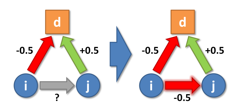
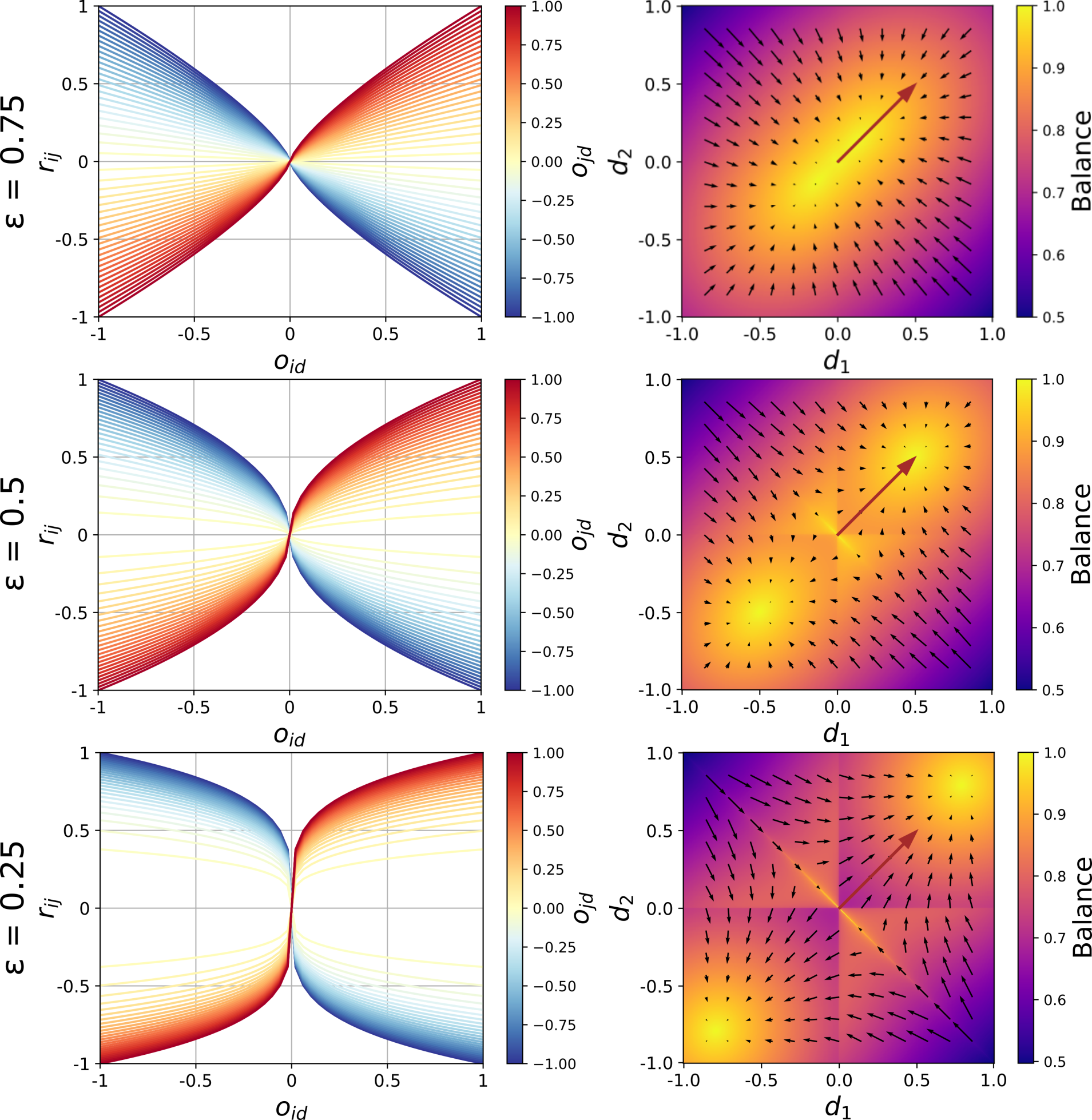
For \(\epsilon > 0.5\), the predicted weight of \(r_{ij}\) will be smaller than the weights of \(o_{id}\) and \(o_{jd}\). For \(\epsilon < 0.5\) it will be larger. An \(\epsilon\) of exactly \(0.5\) gives the geometric mean of \(o_{id}\) and \(o_{jd}\). For this reason, we refer to the above function as Signed Geometric Mean (SGM). Figure 1 illustrates how \(r_{ij}\) is determined as \(-0.5\), given that \(o_{id}=-0.5\), \(o_{jd}=0.5\), and \(\epsilon=0.5\). A low value of \(\epsilon\) represents a tendency to react very emotionally to agreement or disagreement on issues. A person with \(\epsilon < 0.5\) would tend to see the world in a black-and-white, ‘manichean’ way, where "those who are not with me are against me". In contrast, \(\epsilon > 0.5\) represents a calm, emotionally unperturbed reaction to agreement or disagreement. Thus, we refer to \(\epsilon\) as the equanimity parameter. The effect of this parameter is illustrated in the left column of Figure 2. The three line plots depict the relation between the issue positions of individuals \(i\) (x-axis) and \(j\) (line color), and their interpersonal relation \(r_{ij}\) (y-axis), for three different values of \(\epsilon\) (rows). For \(\epsilon=0.75\) (top row), \(r{ij}\) changes in an almost linear way with \(o_{id}\) and \(o_{jd}\). The curves are only slightly steeper when they cross \(o_{id} = 0\). Issue positions of \(i\) and \(j\) are mapped into rather neutral interpersonal relations, in particular when \(o_{id}\) and \(o_{jd}\) are themselves relatively moderate. In contrast, for \(\epsilon=0.25\) (bottom row), the curve have a pronounced sigmoid shape. The relation between \(i\) and \(j\) changes rather abruptly as \(o_{id}\) crosses from negative to positive values, and even relatively weak issue positions are mapped into strong interpersonal attitudes. An animated version of the line plots, depicting equanimity values \(0 < \epsilon < 2\), can be accessed under this link.
Since we want to explain how multiple issues come to align, we need to clarify how Equation 2 should be adapted if there are several issues \(d_1,...,d_D\), with \(D\) being the number of issues. We formalize these various issue positions as a \(D\)-dimensional opinion vector \(\mathbf{o}_i\). In this case, there is still only one interpersonal attitude \(r_{ij}\), but this attitude is now influenced by agreement and disagreement between \(i\) and \(j\) on multiple issues, each forming the apex of their own \(i,j,d\) triad (see Figure 3, left). A priori, we assume that the various influences on \(r_{ij}\) are independent from each other. Thus, we propose that they should simply be averaged:
| \[ r_{ij} = \frac{1}{D}\sum_{d=1}^{D} \text{sign}(\mathbf{o}_{id} \cdot \mathbf{o}_{jd})|\mathbf{o}_{id} \cdot \mathbf{o}_{jd}|^\epsilon\] | \[(3)\] |
Figure 3 illustrates how this process works with two issue dimensions, given that \(\epsilon = 0.5\). Individuals \(i\) and \(j\) disagree about issue \(d_1\), which \(i\) has a negative, and \(j\) a positive attitude towards. However, they both agree on their negative attitude towards \(d_2\). Since the absolute weight of their attitudes towards \(d_2\) is somewhat stronger than towards \(d_1\), \(i\) forms a mildly positive interpersonal attitude towards \(j\).
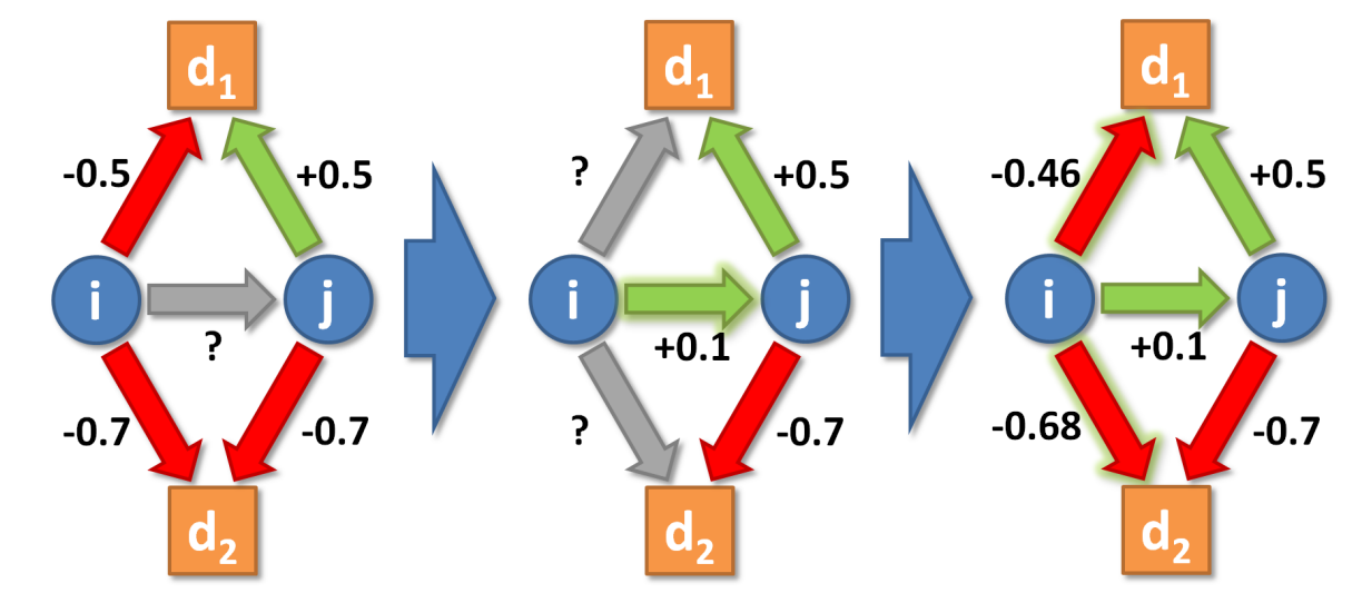
But this is only the first step: Once \(r_{ij}\) is obtained, it forms the basis of the two \(i,j,d\) triads, which are not necessarily balanced. Thus, in the second step, \(i\) will adapt its issue positions in a way that makes them more consistent with its attitude towards \(j\). The pressure to adapt is especially high for the \(i,j,d_1\) triad in our example, since this triad is now very unbalanced: \(i\) and \(j\) disagree on \(d_1\), even though they have a positive relationship.
We postulate that the opinion vector \(\mathbf{o}_{i}\) changes through the SGM (Equation 2) as well, but this time taking \(r_{ij}\) and \(\mathbf{o}_{j}\) as arguments. In this way, we can determine what \(i\)’s issue positions should be in order to achieve cognitive balance, given \(i\)’s feelings towards \(j\) and \(j\)’s issue positions. The result is a maximally balanced opinion vector \(\mathbf{b}_{ij}\) of issue positions, with the same dimensionality as \(\mathbf{o}_i\):
| \[ \mathbf{b}_{ijd} = \text{sign}(r_{ij} \cdot \mathbf{o}_{jd})|r_{ij} \cdot \mathbf{o}_{jd}|^\epsilon\] | \[(4)\] |
If \(r_{ij}\) is positive, \(\mathbf{b}\) will contain issue positions largely agreeing with \(\mathbf{o}_{jd}\). If \(r_{ij}\) is negative, the components of \(\mathbf{b}\) will have the opposite sign of \(\mathbf{o}_{jd}\). For our example (Figure 3), given \(r_{ij} = 0.1\) and \(\mathbf{o}_{j} = [0.5, -0.7]\), we obtain a (rounded) balanced vector \(\mathbf{b} = [0.22, -0.27]\).
However, we do not assume that \(i\) will abruptly change its opinion vector so that \(\mathbf{o}_{i} = \mathbf{b}\), which would mean that \(i\) completely abandons its initial issue positions. Instead, we assume a certain ‘issue position inertia’. Due to this inertia, \(\mathbf{o}_{i}\) will only move by a certain fraction \(\alpha\) towards \(\mathbf{b}\), with \(\alpha\) being a real number between \(0\) and \(1\). The change in \(i\)’s opinion vector, \(\Delta \mathbf{o}_i\), is thus defined as:
| \[ \Delta \mathbf{o}_i = \alpha (\mathbf{b} - \mathbf{o}_i)\] | \[(5)\] |
With \(\alpha = 0.05\) (the same value as in our opinion dynamics model below), \(i\)’s issue position regarding \(d_1\) changes from \(\mathbf{o}_{i1}=-0.5\) to (rounded) \(\mathbf{o}_{i1}=-0.464\) (\(\Delta \mathbf{o}_{i1} = +0.036\)), and \(i\)’s issue position regarding \(d_2\) from \(\mathbf{o}_{i2}=-0.7\) to \(\mathbf{o}_{i2}=-0.678\) (\(\Delta \mathbf{o}_{i2} = +0.022\)). The change in \(\mathbf{o}_{i1}\) is easy enough to comprehend: The triad \(i,j,d_1\) represents a disagreement between friends, which is clearly unbalanced. By weakening its negative attitude towards \(d_1\), \(i\) is trying to reduce this imbalance. The reason for the change in \(\mathbf{o}_{i2}\) is less obvious, since the signs of the triad \(i,j,d_2\) are already balanced, representing agreement between friends. However, the positive attitude of \(i\) towards \(j\) is actually very weak (\(r_{ij}=0.1\)). This weak interpersonal relation creates imbalance with the rather strong attitudes of both \(i\) and \(j\) towards \(d_2\). Thus, here too, the absolute weight of \(\mathbf{o}_{i2}\) is lowered, albeit to a lesser degree than \(\mathbf{o}_{i1}\).
The vector field plots in the right column of Figure 2 illustrate the process of opinion exchange for three different values of the equanimity parameter \(\epsilon\). The axes of the plots span a 2-dimensional opinion space. The red arrow corresponds to the opinion vector \(\mathbf{o}_{j} = [.5,.5]\). The bases of the black arrows correspond to the initial opinion vectors of various individuals \(i = 1,...,N\). The length and direction of the black arrows represent their change in issue position after an interaction with \(j\) (the step size parameter is set to \(\alpha=0.15\) here). The background color represents the level of balance in each region of the opinion space. We define the balance of \(i\) in its interaction with \(j\) as the inverse of the normalized Euclidean distance (\(\text{dist}_e\)) of \(i\)’s opinion vector from its maximally balanced vector:
| \[ \text{Balance}(i,j) = 1 - \frac{\text{dist}_e(\mathbf{o}_i,\mathbf{b}_{ij})}{2\sqrt{D}}\] | \[(6)\] |
Looking at the vector field in the middle row (\(\epsilon=0.5\)), we observe that \(\mathbf{o}_j\) creates a ‘balance landscape’ with two maxima, one at its own location, and one at the opposite location \(-\mathbf{o}_j\) (we ignore the third maximum around the center of the opinion space, since it constitutes an unstable equilibrium point). This means, if an individual \(i\) repeatedly adjusts its opinion vector to \(j\) (with \(\mathbf{o}_j\) remaining stable), \(\mathbf{o}_i\) will eventually end up at one of these two equilibrium points. As can be seen in these animated vector field plots, the equilibrium points don’t always coincide with \(\mathbf{o}_j\) and \(-\mathbf{o}_j\). If \(\mathbf{o}_j\) is not already on a diagonal through the opinion space, the equilibrium points tend to be closer to the nearest diagonal. Which of the two equilibrium points \(\mathbf{o}_i\) approaches depends on the angle between the initial \(\mathbf{o}_i\) and \(\mathbf{o}_j\). An angle smaller than 90° will result in convergence to \(\mathbf{o}_i\), a larger angle in convergence to \(-\mathbf{o}_i\). The angle between \(\mathbf{o}_i\) and \(\mathbf{o}_j\) is also relevant for the change in the vector norm \(||\mathbf{o}_i||\), which we can interpret as the extremeness of an individual’s issue positions. If this angle is around 90°, \(||\mathbf{o}_i||\) will decline. In other words, if two individuals agree on some issues but disagree on others, they will adapt their opinions to become more moderate. If they agree or disagree on most issues (i.e., the angle between \(\mathbf{o}_i\) and \(\mathbf{o}_i\) is closer to 0° or 180°), \(||\mathbf{o}_i||\) will tend to ‘match’ \(||\mathbf{o}_j||\), meaning if \(i\)’s attitudes are more extreme than \(j\)’s, \(i\) will become more moderate, and vice versa.
Changing the equanimity parameter \(\epsilon\) causes a shift in the location of the two equilibrium points: If \(\epsilon > 0.5\) (top row, \(\epsilon = 0.75\)), the equilibrium points are closer to the center of the opinion space, and at some point even merge. This leads to a general tendency towards more moderate views. In contrast, if \(\epsilon < 0.5\) (bottom row, \(\epsilon = 0.5\)), the equilibrium points are shifted outwards, meaning that \(i\) will tend to ‘outdo’ \(j\) in terms of extremeness. An animated vector field plot, visualizing equanimity values \(0 < \epsilon < 1\), can be found here.
The vector field plots in Figure 2 give us a good intuition of how the mechanisms of Weighted Balance Theory might give rise to polarization and issue alignment. But it is crucial to understand that the depicted balance landscape is generated by a specific individual \(j\), in combination with a specific \(\epsilon\) parameter. Other individuals will give rise to different landscapes. It remains to be seen whether the mechanisms postulated by our Weighted Balance Theory – determining interpersonal attitude based on issue positions, and adapting issue positions based on interpersonal attitude – can give rise to the emergence of a single ideological spectrum in a high-dimensional opinion space. In the following two sections, we answer this question by implementing WBT into an agent-based opinion dynamics model.
Implementation of the Weighted Balance Model
The central question of this study is whether the mechanisms of WBT are sufficient to generate issue alignment and polarization. If we simulate a population of agents repeatedly interacting with each other based on the mechanisms of WBT, will a single ideological spectrum eventually arise from an initially random state? And under which parameter constellations will this happen?
We simulate our model for a population of \(N\) agents, which have positions on \(D\) issue dimensions. These issue positions are captured in a \(N\) by \(D\) opinion matrix \(\mathbf{O}\). At the beginning of each model run, the components of \(\mathbf{O}\) are drawn from a random uniform distribution bounded between \(-1\) and \(1\). The model will then run over \(T\) timesteps. At each timestep \(t\), each of the \(N\) agents interacts with a randomly chosen other agent, such that no agent interacts with itself.
As described in Section 3, an interaction proceeds in two steps: 1) forming an interpersonal relation based on issue positions (Equation 3), and 2), adapting issue positions based on the interpersonal relation (Equations 4 and 5). For simplicity’s sake, we model these interactions as one-sided, meaning agent \(i\) adapts its issue positions to agent \(j\), but not vice versa (we have tested models with mutual interactions, and found they produce very similar results). We also make the simplifying assumption that agents form their relations and adapt their positions over all \(D\) issue dimensions simultaneously. However, our model does not produce qualitatively different outcomes as long as agents form their relation on at least two issue dimensions. With fewer issue dimensions on which agents interact, the model merely takes longer to converge. Only if agents interact on just a single issue dimension, the model behavior breaks down, because now the opinion dynamics on different issue dimensions is effectively decoupled.
At each timestep \(t\), we add noise, drawn from a random normal distribution with mean \(0\) and standard deviation \(\zeta\), to each component of the opinion matrix \(\mathbf{O}\). This noise reflects influences on the issue positions of individuals which cannot be captured by our model dynamics (such as personal experiences, private deliberations etc.). It is good practice to implement noise into opinion dynamics models, since the predictive power of a model which collapses under even moderate degrees of noise is questionable. It may occur that, through the addition of random noise, some opinion vectors leave the confines of the opinion space. If this happens, we ‘reflect’ them back into the space, by subtracting the distance by which they would exceed the confines of the opinion space from the borders of the space.
For all of our model runs, we keep the parameter \(\alpha\), which controls the speed of opinion change in a given interaction, to the relatively small value of \(\alpha=0.05\). We believe a small value of \(\alpha\) is realistic, since people rarely change their opinions completely in reaction to a single conversation with another person. Another parameter we keep constant is the number of timesteps in each model run, which we set to \(T=3000\). However, even in the absence of random noise, the model never comes to rest completely, which makes it difficult to apply a convergence criterion.
The most important parameter of our model is the equanimity parameter \(\epsilon\). In our previous paper (Schweighofer et al. 2020), we explored the model behavior under a singular value of the \(\epsilon\) parameter for all agents. Under this assumption, the model produced two distinct outcomes: a complete consensus with all agents in the center of the opinion space or a fully polarized state with the agent population separating into two relatively equal groups, which then migrate to two opposite corners of the opinion space. While these outcomes confirmed that a WBT-based model can produce polarization, the distribution of positions we obtained is still quite unrealistic, as real political systems are rarely in a state of complete polarization or complete consensus. In this study, we relax the assumption of a uniform \(\epsilon\) for all agents and include an individual-specific value of \(\epsilon\), represented in our model as an N -dimensional vector \(\mathbf{e}\).
For each agent, we draw a random \(\epsilon\)-value from a log-normal distribution with mean \(\mu_\epsilon\) and standard deviation \(\sigma_\epsilon\), and divide the resulting value by 2. In this way, if \(\mu_\epsilon=0\), we obtain a a log-normal distribution with a median of \(0.5\), representing the ‘neutral’ value of \(\epsilon\). Negative values of \(\mu_\epsilon\) represent distributions where the typical agent has a ‘manichean’ tendency (\(0 \leq \epsilon < 0.5\)), while positive values of \(\mu_\epsilon\) result in a population of largely equanimous agents (\(\epsilon > 0.5\)). The reason for sampling from a log-normal distribution is that empirically estimated \(\epsilon\)-values are distributed in a long-tailed, heavily skewed fashion (see Section 7, Figure 7, left).
We use three metrics to assess the final state of a model run: Alignment, Extremeness, and Polarization. Each metric is scaled between \(0\) and \(1\). Alignment quantifies how much variance of the agents’ issue positions can be explained by a single underlying ideological dimension. It is based on the first eigenvalue \(\lambda_1\) of the covariance matrix derived from the opinion matrix \(\mathbf{O}\). We rescale the eigenvalue, so that \(\lambda_1=1\) (the minimal possible value) corresponds to \(Alignment=0\), and \(\lambda_1=D\) corresponds to \(Alignment=1\):
| \[ \text{Alignment}(\mathbf{O}) = \frac{\lambda_1 - 1}{D-1}\] | \[(7)\] |
For Extremeness, we compute the arithmetic mean of the magnitudes of all opinion vectors, and normalize it between \(0\) and \(1\):
| \[ \text{Extremeness}(\mathbf{O}) = \frac{1}{N\sqrt{D}} \sum_{i=1}^N||\mathbf{O}_{i}||\] | \[(8)\] |
Both Alignment and Extremeness capture certain aspects of polarization but do not give us the whole picture. For this purpose, we construct a polarization index (see Schweighofer et al. 2020). Following the conventions of political science, our polarization index is based on the matrix of issue positions \(\mathbf{O}\), and not on agents’ interpersonal attitudes. The polarization index is based on the definition of a maximally polarized state as comprising two groups of equal size, which are maximally opposed to each other, and maximally coherent internally (Bauer 2019; Galtung 1996). In terms of our model, this would correspond to two groups of \(N/2\) agents inhabiting diametrically opposed corners of the opinion space. This distribution is the only one for which the sum of squared distances between agents is maximal, which we capture in our Polarization metric:
| \[ \text{Polarization}(\mathbf{O}) = \frac{4}{N^2d_{max}} \sum_{i=1}^N\sum_{j=1}^i d_e(\mathbf{O}_{i},\mathbf{O}_{j})^2\] | \[(9)\] |
Analyzing the Role of Equanimity in the WBT Model
Figure 4 shows the Polarization of the opinion matrix \(\mathbf{O}\) produced by model runs with varying mean (\(\mu_\epsilon\), x-axis) and standard deviation (\(\sigma_\epsilon\), color) of the equanimity parameter \(\epsilon\). As mentioned, these are the mean and standard deviation of a random normal distribution, which is then exponentiated and divided by 2 to give us the \(\epsilon\)-parameters of individual agents. Each dot represents the degree of polarization in the end state of a model run (at \(t=3000\)).
Figure 4 a shows model runs without noise (\(\zeta=0\)). If we focus on the model runs with no individual variation in equanimity (\(\sigma_\epsilon=0\); dark blue color), we can see that they reproduce the outcomes of our previous study (Schweighofer et al. 2020): Model runs with negative mean equanimity (\(\mu_\epsilon < 0\)) result in a completely polarized state, where the agent population is separated into two equal groups in opposite corners of the opinion space. But polarization drops abruptly at \(\mu_\epsilon = 0\). For \(\mu_\epsilon \geq 0\), polarization is zero, meaning all agents have converged to the center of the opinion space.
This sudden transition, however, becomes smoother with higher values of \(\sigma_\epsilon\). For model runs with \(\sigma_\epsilon=2\) (yellow color), polarization declines gradually with increasing \(\mu_\epsilon\). Thus, by giving the agents heterogeneous individual equanimity values, the model is able to generate a broader range of degrees of polarization, which increases the realism of the model. While the results shown here are for \(D=5\), we have reproduced this behavior for much higher numbers of issue dimensions, all the way to \(D=1000\), which probably far exceeds the number of salient policy issues discussed in a general election.
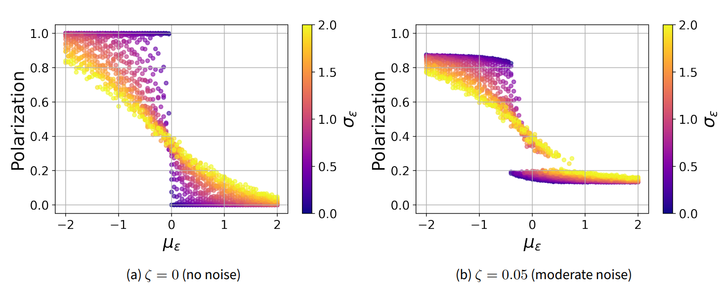
Figure 4 b shows the effects of noise on the model behavior. First, we notice that the model can no longer reach full polarization or complete consensus. These idealized opinion configurations are disturbed by the influence of noise. For models with uniform equanimity parameter (\(\sigma_\epsilon=0\)), there is still a sudden drop in polarization. However, this drop now happens at a slightly lower value of mean equanimity (around \(\mu_\epsilon=-0.5\)).
On the other hand, even model runs with very heterogeneous equanimity distribution now exhibit a drop in polarization at varying thresholds, resulting in a ‘gap’ of polarization values of varying width (depending on \(\sigma_\epsilon\)). This gap is due to noise keeping the agents from aligning themselves to a single ideological spectrum in the early phase of the model. The lack of issue alignment forestalls any trend toward more polarization. If a society has oscillations between positive and negative \(\mu_\epsilon\) values, this can create a hysteresis cycle with sudden jumps towards a polarized state when equanimity goes below a critical value.
Figure 5 illustrates three idiosyncratic model runs. Each of these models has been run with our usual settings (see above), \(D=3\) and \(\sigma_\epsilon=1\). The only difference between them is the mean of the agent-specific equanimity distribution (\(\mu_\epsilon\)), which results in very different degrees of polarization: \(0.14\) for the model with \(\mu_\epsilon=0.5\) (top), \(0.35\) for the model with \(\mu_\epsilon=0\) (middle), and \(0.71\) for model with \(\mu_\epsilon=-0.5\) (bottom).
The varying levels of mean equanimity also result in very different distributions of positions along the first three issue dimensions (see histograms): the model run with \(\mu_\epsilon=0.5\) (top) produces a normal distribution with a clear peak around 0. Thus, most agents end up with relatively neutral issue positions. Only agents with very low equanimity polarize to a certain degree, but even they are kept near the center by the ‘pull’ of the neutral agents. Most of the agents in the model run with \(\mu_\epsilon=0\) (middle) are still near the center of the opinion space, but they are now flanked by two ‘wings’ with more extreme positions. Finally, the model run with \(\mu_\epsilon=-0.5\) (bottom) produces a opinion distribution which bears clear signs of polarization: The center has shrunk, and the two ‘wings’ have become more extreme, and more popular.
We can also look at differences in the model evolution: The line plots on the bottom of each panel of Figure 5 illustrate the development of Alignment, Extremeness, and Polarization (animated versions of the three model runs under this link). All three model runs (and indeed every model run independent of parameter settings) start with a steep decline of Extremeness and Polarization (Alignment already starts out low). This is due to the initial random positions of the agents, which imply that most agents are neither agreeing nor disagreeing on a majority of issues. As we know from our discussion of the vector field plots in Section 3 (Figure 2, right column), if agents with more or less orthogonal opinion vectors interact, the magnitude of opinion vectors declines. Thus, our simulated agents converge to the center of the opinion space at around timestep \(t=50\).
How long the system remains in this state of low polarization depends on the parameter settings. In the model run with \(\mu_\epsilon=-0.5\) (bottom), this depolarized state only lasts for about 50 time steps. During this phase, the agents organize themselves into a single, dominant ideological spectrum, a process reflected in the steep increase in Alignment, preceding the increase of Extremeness and Polarization. Again, looking back at the vector field plots in Figure 2 (right column) can help us explain this process: Due to random chance, some quadrants of the opinion space will be populated by more agents than others. When they interact with other agents, they will either pull them towards their own or push them to the opposite quadrant. This initiates a self-reinforcing process, where more and more agents populate a specific diagonal through opinion space, exerting a stronger and stronger combined force on the remaining ‘unaligned’ agents. This force is stronger for agents with low equanimity. Consequently, in the model run with \(\mu_\epsilon=0\) (middle), the process of opinion alignment takes much longer (around 200 time steps), which also entails a longer depolarized state. Eventually, however, Alignment reaches almost perfect levels. Finally, in the model run with \(\mu_\epsilon=0.5\) (top), the alignment process takes around 700 time steps, and never reaches the same high level as in the other two model runs.
Once the agents are sufficiently aligned, Extremeness and Polarization increase again, and then remain stable at a higher level (although in the case of \(\mu_\epsilon=0.5\) only slightly higher). Yet another look at vector field plots in Figure 2 (right column) can help us understand this polarizing phase. Now that all agents are aligned along the same diagonal, a different self-reinforcing dynamics sets in: Agents with low equanimity parameter (\(\epsilon < 0.5\)) will ‘leapfrog’ each other, thus collectively moving to the extreme corners of the opinion space. However, they will be held back by moderate agents with high equanimity parameter (\(\epsilon > 0.5\)), who exert a pull towards the center of opinion space (but are themselves pulled outwards by more extreme low-equanimity agents).
Thus, we always find agents with high \(\epsilon\) at the center, and agents with low \(\epsilon\) at the fringes of our emergent ideological spectrum (see Figure 5). Where exactly these fringes are though is determined by the mutual attraction and repulsion of agent populations with different \(\epsilon\)-values. Due to this constant push and pull, the equilibrium that the model eventually reaches is not static, but very dynamic. As we show in Appendix A, even without artificial noise, agents never completely come to rest, but oscillate around an average position on the ideological spectrum.
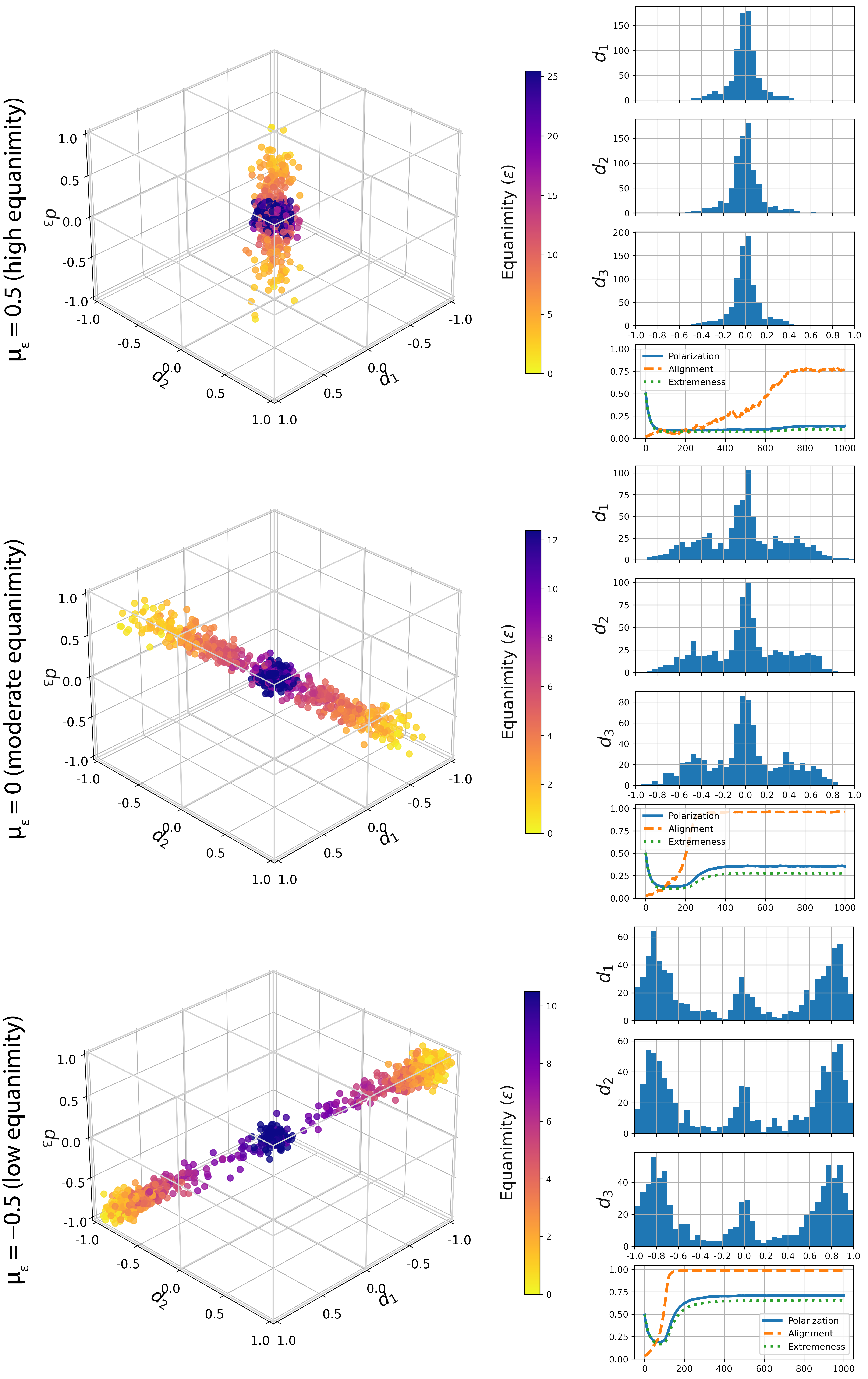
Beyond the degrees of Polarization, the three model runs in Figure 5 also differ in one very conspicuous way. In each of them, an ideological spectrum emerges along a diagonal through the opinion space, but the orientation of the spectrum is always different. This illustrates that along which specific diagonal the ideological spectrum emerges is random, and not in any way dependent on the model parameters, as no mechanism in the model favors one direction over another.
Predicting Interpersonal Attitudes in ANES Data
In Section 3, we have laid out the mechanisms of Weighted Balance Theory. In the Section 4 and 5, we have shown that these mechanisms can give rise to issue alignment and political polarization. But the question remains whether the mechanisms of WBT can be validated empirically. In this section, we use data from the ANES survey to test a central assumption of WBT, namely that interpersonal attitudes can be predicted using the signed geometric mean (SGM) of opinion vectors.
The American National Election Studies (ANES) has repeatedly surveyed representative samples of American voters since 1948. Respondents are polled on a wide variety of socio-demographic attributes, social and policy issues, and attitudes towards politicians and political entities. For our purposes, three types of ANES items are especially relevant, because they correspond to the three relations constituting \(i,j,d\) triads:
- Items asking for respondents’ own positions on a variety of politically relevant issues, which correspond to \(\mathbf{o}_{i}\).
- Items asking respondents to estimate the positions of electoral candidates on these same issues, corresponding to \(\mathbf{o}_{j}\).
- ‘Feeling thermometer scales’, asking for respondents’ feelings towards electoral candidates from ‘cold’ (negative) to ‘warm’ (positive), corresponding to \(r_{ij}\).
Items of type 1 and 2 have seven answer categories, expressing different degrees of approval and disapproval, as well as a neutral category. Feeling thermometer items (type 3) allow ratings from 0 ("very cold or unfavorable feeling") to 100 ("very warm or favorable feeling"). We rescale all items so that the most negative possible answer category corresponds to \(-1\), and the most positive to \(+1\). Based on the rescaled items, we can now test the predictions of Weighted Balance Theory. In particular, we want to see whether knowing respondents own issue positions (type 1 items), as well as their estimates of candidates’ issue positions (type 2), will allow us to correctly predict their feelings towards these candidates (type 3).
In our analysis, we focus on ANES surveys conducted in the run-up to presidential elections, and on attitudes towards presidential candidates from the Republican and Democratic party. However, items of the three types discussed above also exist for congressional election candidates and the two major political parties. In Appendix C, we conduct similar analyses with these entities. Here, we focus on presidential candidates for the simple reason that presidential elections are more salient, and the candidates more present in the media. Thus, we can expect that most respondents have formed some emotions towards the candidates, and have at least a cursory concept of these candidates’ issue positions.
For presidential candidates, items of the three required types are available for every one of the twelve presidential elections from 1972 to 2016. Over the 12 survey waves in this 44 year period, a total of 30,588 respondents were surveyed. Respondents were asked about their feelings towards, and estimates of the issue positions of both major party candidates. In effect, each respondent provides two data points for our estimation of feeling thermometer ratings. However, of the 61,176 data points, 20.3% had to be excluded, because they were either missing the thermometer rating of the candidate, or one or several of the issue position questions. This leaves us with a total sample size of \(N=48,728\). The number of valid cases per presidential election ranges from \(1,755\) (in 2000) to \(10,624\) (2012).
The number and content of items available as both type 1 and type 2, corresponding to the number of issue dimensions \(D\), also varies across election cycles. In 1988, 7 items exist as both type 1 and type 2 version, but in 1992 there were only 3 items. On average, there are \(4.9\) parallel items across the 12 presidential elections of our study. The changing content of the items reflects the change in the political agenda over time, ranging from attitudes towards defense spending to marriage equality. Most items, however, were present across several consecutive waves of the ANES survey, until they were replaced with more topical items.
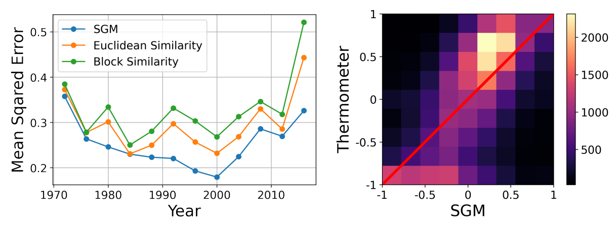
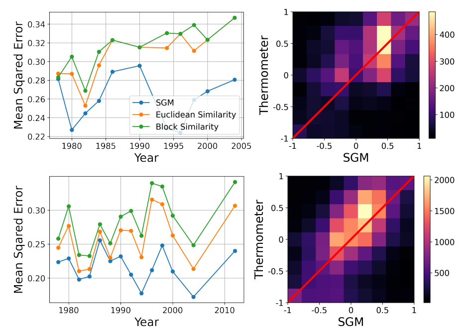
To assess the quality of our WBT-based predictions, we compute the mean squared error of the thermometer rating based on the SGM between \(\mathbf{o}_i\) and \(\mathbf{o}_j\). We compare the quality of WBT-based predictions with a benchmark of two other similarity metrics: Euclidean distance and Block distance (aka Manhattan distance). These metrics express the similarity between two opinion vectors \(\mathbf{o}_i\) and \(\mathbf{o}_j\). Euclidean and block distance are commonly used in opinion dynamics models, as well as in political science, to estimate similarity between positions in a multidimensional opinion space. By re-scaling them between \(-1\) and \(1\), we can compare them with corresponding thermometer ratings. With \(\text{dist}_e\) denoting Euclidean distance, the Euclidean similarity metric \(S_e\) is defined as follows:
| \[ S_e = 1- \frac{\text{dist}_e(\mathbf{o}_i - \mathbf{o}_j)}{\sqrt{D}}\] | \[(10)\] |
The block distance (\(\text{dist}_b\)) based similarity metric \(S_b\) is given as:
| \[ S_b = 1- \frac{\text{dist}_b(\mathbf{o}_i - \mathbf{o}_j)}{D}\] | \[(11)\] |
Weighted Balance Theory can be seen as validated if the SGM can estimate thermometer ratings with a higher degree of precision than these two metrics. To make the comparison between these different metrics fair, we apply all three of them without any parameter tuning. This means that for the SGM, we use a fixed \(\epsilon=0.5\) for all respondents and survey waves. The results of this comparison can be seen in Figure 6 (left). Over each of the 12 ANES survey waves, the SGM estimate produces a smaller mean squared error than Euclidean and block distance based similarity metrics. This means that the SGM produces a consistently better estimate of respondents’ thermometer ratings of presidential candidates than the two benchmark metrics.
The quality of the WBT-based prediction can also be seen in Figure 6 (right), which shows the SGM-based estimate and empirical thermometer ratings for all twelve survey waves combined. The diagonal line represents a perfect prediction of respondents’ thermometer ratings by the SGM. It can easily be seen that most cases are very close to this line, whereas the bottom right and top left corner, which would represent the worst prediction errors, are completely devoid of cases. We obtained similar results for our respondents’ attitudes towards political parties and congressional candidates (see Appendix C).
Reproducing Empirical Polarization Levels
In Section 5, we have run our model using randomly generated equanimity (\(\epsilon\)) values. We have seen that these model runs produce results that are qualitatively similar to the ‘stylized facts’ of political polarization. In this section, we want to see whether we can go beyond mere qualitative similarity and actually use our model to reproduce empirical observations through quantitative validation. Instead of synthetic distributions, we use empirical estimates of individual Equanimity (\(\epsilon\)) based on ANES survey data. We do this to explore whether our model, when calibrated with these \(\epsilon\)-values, is able to generate opinion distributions with a degree of polarization that resembles the empirical degree of polarization measured with ANES data.
To calibrate our model, we estimate individual \(\epsilon\)-parameters based on the same ANES data which we already investigated in the last section. Our estimation process minimizes the squared error, i.e. the squared distance of the SGM based prediction and the empirically measured thermometer rating. For example, if a respondent has a more extreme attitude towards a candidate than predicted with \(\epsilon = 0.5\), we adjust \(\epsilon\) to a lower value until we have minimized the squared error. Fortunately, this problem is convex, so we use a gradient descent algorithm to find the optimal value for each respondent. We apply this algorithm to each of the twelve ANES survey waves. Figure 7 (left) shows the distribution of \(\epsilon\)-values for the 2016 wave. Each of the resulting distributions of individual \(\epsilon\)-values is extremely skewed: While the median ranges between \(0.32\) and \(0.6\), the mean is between \(2.42\) and \(4.85\). The minima are always close to zero, whereas the maximum values can go as high as \(\epsilon=45.1\). We thus have distributions of individual \(\epsilon\) that are asymmetric and long-tailed. As explained in Section 4, we emulate these skewed distributions in our model by drawing \(\epsilon\) values from a log-normal distribution.
We can now use the empirically estimated \(\epsilon\) values to calibrate our model. We incorporate these values into our model so that each simulated agent corresponds to an individual ANES respondent. Thus, the number of agents \(N\) of the simulation corresponds to the number of respondents in the ANES survey. Furthermore, we also take over the number of issue dimensions \(D\) from the number of items in the ANES survey, which vary from 3 (in 1992) to 7 (in 1988; see Table 1 in Appendix B).
However, we do not take over respondents’ opinion vectors. Instead, agents’ opinion vectors are initiated with random uniform values. One parameter which we cannot estimate based on the empirical data is the noise parameter \(\zeta\). We explore 11 different noise levels, from \(\zeta=0\) to \(\zeta=0.1\). For each noise level and for each of the twelve ANES waves from 1972 to 2016, we compute 40 separate simulations, for a total of 5,280 simulations. We then compare the averaged results of the simulations to the properties of the empirical ANES opinion distributions. In particular, we evaluate the results based on the mean squared error and correlation between empirically measured and simulated Polarization across waves.
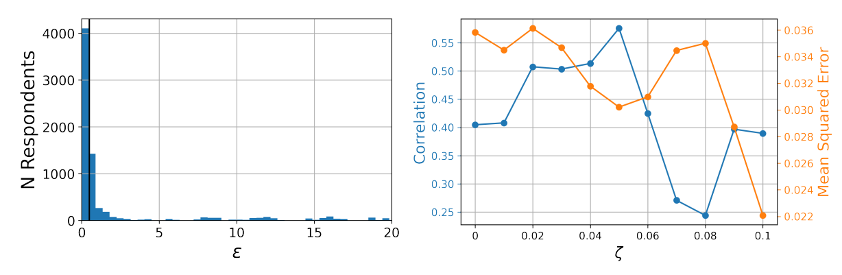
The results can be seen in Figure 7 (right): correlation between simulated and measured polarization is high for all levels of noise, but reaches a maximum of \(r=0.86\) (\(p<0.001\)) at \(\zeta=0.05\). For this noise level, the mean squared error also reaches a local minimum. While mean squared error declines to even lower levels for \(\zeta \geq 0.09\), it does so at a much lower correlation. We therefore select \(\zeta=0.05\) as a suitable level of noise to reproduce the empirical time series of polarization with our WBT model, calibrated on the empirical distribution of \(\epsilon\)-values.
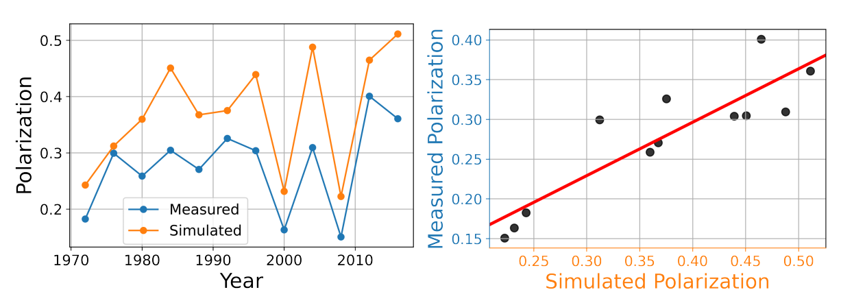
Figure 8 gives a visual impression of the concordance between Polarization measured on ANES data, and simulated with our Weighted Balance Model with \(\zeta=0.05\). While there is a difference in the level of polarization throughout the time series, with simulated Polarization values always being higher than empirical Polarization, the trajectories of simulated and empirical Polarization are very similar. Thus, the WBT model is able to explain trends in Polarization based only on changes in the distribution of the individual \(\epsilon\) parameter.
Discussion
Our outcomes have demonstrated several points: First, we have demonstrate that an opinion dynamics model based on the precepts of Weighted Balance Theory can generate opinion alignment and polarization in arbitrarily high-dimensional opinion spaces. When the assumption of a uniform level of equanimity is relaxed, and replaced by an individual-specific \(\epsilon\)-parameter, our model is able to produce much more realistic distributions of ideological positions, with a gradual change, rather than a sudden shift from complete consensus to total polarization (as was the case in our previous model, see Schweighofer et al. 2020). What degree of polarization is realized depends chiefly on the mean and standard deviation of the distribution of agent-specific equanimity values (\(\epsilon\)).
Second, we have shown that the balance mechanism at the heart of Weighted Balance Theory can be used to predict the attitudes of ANES survey respondents towards presidential candidates, based only on their own issue positions and their estimates of candidates’ positions. What’s more, WBT-based estimates are closer to empirically measured attitudes than estimates based on Euclidean or Block distance. Beating these benchmarks is important, because these distance metrics are frequently used in Opinion Dynamics Modeling, as well as in political science (Laver 2014).
Finally, by calibrating our model with empirically estimated agent-specific \(\epsilon\)-values, we have demonstrated that the model can reproduce the changes in Polarization observed in twelve successive waves of ANES data. To us, this result is the most remarkable: to reiterate, we only take over two global parameters, \(N\) and \(D\), and one individual-level parameter, equanimity (\(\epsilon\)), from ANES data. The actual issue positions of ANES respondents do not inform our model in any way.
We obtain these results even though our model is rather simplistic: We deliberately chose not to model any specific neighborhood or network structure. While these would be more realistic, they would add unnecessary complications and assumptions to our model, and make it more difficult to assess its generative sufficiency. Instead, we adopt a mean field approach, i.e. each pair of agents has an equal probability to interact.
Furthermore, it would be reasonable to assume that not only different individuals may have different levels of equanimity, but that also some policy issues can be more controversial and divisive than others (for a more detailed treatment of these aspects, see Baumann et al. 2021). To keep the model as simple as possible, we have ignored this option for now. However it would be easy to adapt the model by changing the equanimity vector \(\mathbf{e}\) into a \(N\) by \(D\) matrix \(\mathbf{E}\).
At this point, we have to stress again that Cognitive Balance Theory is concerned with cognitive representations and processes taking place in individual \(i\)’s mind. This includes the opinion vector \(\mathbf{o}_{j}\), which does not necessarily represent the actual issue positions of individual \(j\), but rather \(i\)’s beliefs about \(j\)’s issue positions. It is reasonable to assume that the cognitive representation of \(\mathbf{o}_{j}\) is not a complete product of \(i\)’s fantasy, wholly disconnected from \(j\)’s actual issue positions. Nevertheless, there is a possibility that \(i\), instead of adapting its own issue positions, will try to increase balance by systematically misrepresenting \(j\)’s positions. For example, if \(i\) likes \(j\), \(i\) might simply choose to believe that they agree on most issues, even if this is not the case. This is especially plausible if the information \(i\) has on \(j\)’s positions is ambiguous or incomplete.
In our opinion dynamics model, we ignore this possibility, and assume that \(i\) represents \(\mathbf{o}_{j}\) correctly, and increases balance by adjusting its own issue positions, rather than its representation of \(\mathbf{o}_{j}\). However, in our analysis of empirical data from the American National Election Studies, it is likely that part of the observed agreement between respondents’ own opinions, attitudes towards presidential candidates, and beliefs about these candidates’ opinions, stems from the respondents systematically misrepresenting the issue positions of the candidates. In future studies, we plan to investigate whether respondents’ beliefs about candidates’ issue positions are really biased in the systematic way that WBT would suggest.
In the spirit of this special issue, we want to voice a few thoughts about the general direction of opinion dynamics modeling: We believe that, in general, much higher importance needs to be attached to empirical validation, i.e. to the validation of model assumptions and model results with empirical research. Without the ‘selection pressure’ of empirical validation, models will just continue to proliferate in a very chaotic manner. Only a systematic comparison with empirical data makes it possible to cumulatively increase the explanatory power of our best models – and discard models whose explanatory power is insufficient.
The validation of model results should be conducted on two levels: the macro-phenomena generated by the model and the micro-mechanisms on which the model rests. When we model a new phenomenon, we often have to do this in the form of ‘stylized facts’, since it would be asking too much to reproduce empirical data perfectly from the outset. But all too often, research in our field gets stuck in this early stage. Instead of gradually superseding the initial, simplistic models with ones that have higher explanatory power, we continue producing models that all just generate the same stylized facts.
The principles informing a model’s micro-mechanisms cannot be treated merely as convenient fictions, but have to be taken seriously as theoretical assumptions. Micro-mechanisms cannot only be judged by their usefulness for modeling a certain macro-phenomenon, but have to be tested empirically in their own right. If they cannot be validated empirically, they have to be discarded, no matter how successful they are in generating interesting model behavior. Furthermore, micro-mechanisms should not be invented ad hoc by the modeler, and exist only within the confines of a single paper, but should be borrowed from an empirical theory (for example from the social sciences, psychology, or economics).
We believe that the greatest value of Agent-Based (ABM) and Opinion Dynamics Models (ODM) consists in their role as a tool for deductive reasoning. ABMs and ODMs can help us explore to which macro-phenomena a theory gives rise. In other words, they allow us to assess the generative sufficiency of a theory (Epstein 2012). Currently, the field of ABM and ODM suffers from relative isolation from empirical disciplines, which rarely integrate or even acknowledge modeling research. Anchoring our models in empirical theories can enable us to ‘speak the same language’, and thus enter a more productive dialogue with disciplinary scientists. While their empirical insights can help us refine and calibrate our models, we can assist them in formalizing their theories and uncover new ways in which their theoretical assumptions can be validated.
Conclusion
Political polarization is endangering the stability of democratic societies. While polarization is often conceptualized as extremeness of opinions, truly polarized states can only emerge when various policy issues are aligned with each other, merging into one dominant ideological spectrum. In this study, we have set out to explain how alignment can emerge from initially uncorrelated issue positions, and give rise to extremism and polarization. The foundation for our explanatory approach is Weighted Balance Theory, a further development of Fritz Heider’s Cognitive Balance Theory, taking into account weighted attitude relations.
We first construct an opinion dynamics model on the principles of WBT and show that this model can indeed give rise to issue alignment and varying degrees of extremeness and polarization. We then empirically validate WBT by showing how it can be used to predict respondents’ attitudes toward presidential candidates in 42 years worth of survey data from the American National Election Studies. Finally, we calibrate our model with empirical data from the ANES survey and demonstrate that this calibrated model generates levels of polarization that parallel the levels observed in the empirical data.
We believe it is remarkable that our model, despite its relative simplicity, is able to reproduce empirical results to such a degree of precision, and hope that these results can inspire other researchers to test the precepts of Weighted Balance Theory, both computationally and empirically.
Appendix A: Timlines of Individual Agents
Figure 9 depicts the changes in issue positions over the course of a model run (\(T=3000\)) for three individual agents, whose equanimity values are close to \(\epsilon = 0.75\) (left), \(\epsilon = 0.5\) (middle), and \(\epsilon = 0.25\) (right). The model was run with \(D=3\) issue dimensions, \(\mu_\epsilon=0\) and \(\sigma_\epsilon=1\). It is therefore similar to the model in Figure 5 (middle). The only difference is that the model here was run without noise (\(\zeta=0\)), to make it clear that agents’ issue positions never stop oscillating, even in the absence of exogenous noise.
At \(t=0\), all three agents start with random values of their three issue positions \(\mathbf{O}_{i1}\), \(\mathbf{O}_{i2}\), \(\mathbf{O}_{i3}\). Over the next 100 time steps, they converge to the center of the opinion space. As explained in Section 5, in this de-polarized phase, the agents self-organize into an emergent ideological spectrum. We can see this happening in Figure 9, with some lines crossing the x-axis.
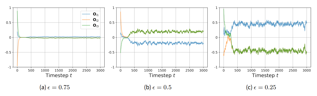
Once the self-organization is complete (around \(t=400\)), issue positions become more extreme again. How extreme depends on the individual level of equanimity of the agent, with lower levels corresponding to more extreme positions. As mentioned, we can also see that issue positions never stop oscillating, although around a stable, individual-specific level. Oscillations are greater for agents with lower equanimity-values. Also, the issue positions of a given agent are now in ‘lock-step’: \(\mathbf{O}_{i2}\) and \(\mathbf{O}_{i3}\) are superimposed on each other, and their movement is mirrored by \(\mathbf{O}_{i1}\). In other words, the agents’ movements are totally bound to the emergent ideological spectrum.
Appendix B: Variables Used in the ANES Analyses
| Year | Party | Presidential Candidate | House Candidate |
|---|---|---|---|
| 1972 | AHJW | ||
| 1976 | AHJW | ||
| 1978 | AHJRW | AJW | |
| 1980 | ACDJW | ACDJW | AJW |
| 1982 | ADGJW | AGJW | |
| 1984 | ACDGJ | ACDGJ | GJ |
| 1986 | DG | G | |
| 1988 | ACDGHJW | ACDGHJW | |
| 1990 | ADG | G | |
| 1992 | DGJ | DGJ | |
| 1994 | AGHJ | GJ | |
| 1996 | DG | ADGHJW | G |
| 1998 | GW | GJW | |
| 2000 | ADGJ | ADGJW | G |
| 2004 | ADGJW | ADGJW | G |
| 2012 | GHJ | AGHJ | |
| 2008 | ADGHJW | ||
| 2016 | ADGHJ |
Appendix C: Estimating Attitudes towards House Candidates and Political Parties
In this appendix, we try to replicate the analyses conducted in Section 6 regarding presidential candidates with House candidates and political parties. Just like with presidential candidates, we try to estimate respondents’ attitudes towards House candidates and political parties based on their own issue positions, and their estimates of the issue positions held by the House election candidate or political party.
Over 11 ANES waves, a total of 19,558 respondents where asked about their attitudes towards Republican and Democrat contenders for elections to the House of Representative, and corresponding issue positions. Again, we have two data points per respondent. However, only 21.8% of respondents completed all attitude and issue position items, leaving us whith a much smaller sample size of \(N=8,551\). The situation is much better for the two major political parties: Over 14 ANES waves, 29,997 respondents where asked their attitudes towards the Republican and Democratic Parties, and corresponding issue positions. We have incomplete data points for 26.9% of cases, leaving us with a sample size of \(N=43,849\).
As we can see in Figure 10, for both the attitude towards congressional candidates (top row) and towards political parties (bottom row), the SGM delivers a better estimate for every single ANES survey wave (left column). The closeness of the SGM based estimates to the actual feeling thermometer ratings is further illustrated by the 2-D histograms (right column), which show that most cases are clustered around the diagonal, and no cases occur in the top left and bottom right corners, representing the worst estimation mistakes. All of this is very much in line with our analysis of attitudes towards presidential candidates in Section 6.
References
BALDASSARRI, D., & Gelman, A. (2008). Partisans without constraint: Political polarization and trends in American public opinion. American Journal of Sociology, 114(2), 408–446. [doi:10.1086/590649]
BAUER, P. C. (2019). Conceptualizing and measuring polarization: A review. SocArXiv preprint. Available at: https://osf.io/preprints/socarxiv/e5vp8 [doi:10.31235/osf.io/e5vp8]
BAUMANN, F., Lorenz-Spreen, P., Sokolov, I. M., & Starnini, M. (2020). Modeling echo chambers and polarization dynamics in social networks. Physical Review Letters, 124(4), 048301. [doi:10.1103/physrevlett.124.048301]
BAUMANN, F., Lorenz-Spreen, P., Sokolov, I. M., & Starnini, M. (2021). Emergence of polarized ideological opinions in multidimensional topic spaces. Physical Review X, 11(1), 011012. [doi:10.1103/physrevx.11.011012]
BLAU, P. M., & Schwartz, J. E. (1984). Crosscutting Social Circles: Testing a Macrostructural Theory of Intergroup Relations. New York, NY: Academic Press. [doi:10.4324/9781351313049-4]
CARTWRIGHT, D., & Harary, F. (1956). Structural balance: A generalization of Heider’s theory. Psychological Review, 63(5), 277. [doi:10.1037/h0046049]
CONVERSE, P. E. (1964). The nature of belief systems in mass publics. Critical Review, 18(1), 1–74. [doi:10.1080/08913810608443650]
CRANDALL, C. S., Silvia, P. J., N’Gbala, A. N., Tsang, J.-A., & Dawson, K. (2007). Balance theory, unit relations, and attribution: The underlying integrity of Heiderian theory. Review of General Psychology, 11(1), 12–30. [doi:10.1037/1089-2680.11.1.12]
DELLAPOSTA, D. (2020). Pluralistic collapse: The “oil spill” model of mass opinion polarization. American Sociological Review, 85(3), 507–536. [doi:10.1177/0003122420922989]
EPSTEIN, J. M. (2012). Generative Social Science. Princeton, NJ: Princeton University Press.
ESTEBAN, J.-M., & Ray, D. (1994). On the measurement of polarization. Econometrica, 62(4), 819–851. [doi:10.2307/2951734]
FELICIANI, T., Flache, A., & Mäs, M. (2021). Persuasion without polarization? Modelling persuasive argument communication in teams with strong faultlines. Computational and Mathematical Organization Theory, 27, 61–92. [doi:10.1007/s10588-020-09315-8]
FINKEL, E. J., Bail, C. A., Cikara, M., Ditto, P. H., Iyengar, S., Klar, S., Mason, L., McGrath, M. C., Nyhan, B., Rand, D. G., Skitka, L. J., Tucker, J. A., van Bavel, J. J., Wang, C. S., & Druckman, J. N. (2020). Political sectarianism in America. Science, 370(6516), 533–536. [doi:10.1126/science.abe1715]
FLACHE, A., & Macy, M. W. (2011). Small worlds and cultural polarization. The Journal of Mathematical Sociology, 35(1–3), 146–176. [doi:10.1080/0022250x.2010.532261]
FLACHE, A., & Mäs, M. (2008). Why do faultlines matter? A computational model of how strong demographic faultlines undermine team cohesion. Simulation Modelling Practice and Theory, 16(2), 175–191. [doi:10.1016/j.simpat.2007.11.020]
FLACHE, A., Mäs, M., Feliciani, T., Chattoe-Brown, E., Deffuant, G., Huet, S., & Lorenz, J. (2017). Models of social influence: Towards the next frontiers. Journal of Artificial Societies and Social Simulation, 20(4), 2. https://jasss.soc.surrey.ac.uk/20/4/2.html [doi:10.18564/jasss.3521]
GALTUNG, J. (1996). Peace by Peaceful Means: Peace and Conflict, Development and Civilization. Thousand Oaks: SAGE Publications Ltd. [doi:10.4135/9781446221631]
GESTEFELD, M., Lorenz, J., Henschel, N. T., & Boehnke, K. (2022). Decomposing attitude distributions to characterize attitude polarization in Europe. SN Social Sciences, 2(7), 110. [doi:10.1007/s43545-022-00342-7]
GOLDBERG, A., & Stein, S. K. (2018). Beyond social contagion: Associative diffusion and the emergence of cultural variation. American Sociological Review, 83(5), 897–932. [doi:10.1177/0003122418797576]
HEIDER, F. (1946). Attitudes and cognitive organization. The Journal of Psychology, 21(1), 107–112.
HUMMON, N. P., & Doreian, P. (2003). Some dynamics of social balance processes: Bringing Heider back into balance theory. Social Networks, 25(1), 17–49. [doi:10.1016/s0378-8733(02)00019-9]
KOZLOWSKI, A. C., & Murphy, J. P. (2021). Issue alignment and partisanship in the american public: Revisiting the “partisans without constraint” thesis. Social Science Research, 94, 102498. [doi:10.1016/j.ssresearch.2020.102498]
LAVER, M. (2014). Measuring policy positions in political space. Annual Review of Political Science, 17, 207–223. [doi:10.1146/annurev-polisci-061413-041905]
LEWANDOWSKY, S., Smillie, L., Garcia, D., Hertwig, R., Weatherall, J., Egidy, S., Robertson, R. E., O’connor, C., Kozyreva, A., Lorenz-Spreen, P., Blaschke, Y., & Leiser, M. (2020). Technology and democracy: Understanding the influence of online technologies on political behaviour and decision-making. EUR 30422 EN, Publications Office of the European Union, Luxembourg, 2020. Available at: https://publications.jrc.ec.europa.eu/repository/handle/JRC122023
LORENZ-SPREEN, P., Oswald, L., Lewandowsky, S., & Hertwig, R. (2022). A systematic review of worldwide causal and correlational evidence on digital media and democracy. Nature Human Behaviour, 7, 1–28. [doi:10.1038/s41562-022-01460-1]
MARVEL, S. A., Kleinberg, J., Kleinberg, R. D., & Strogatz, S. H. (2011). Continuous-time model of structural balance. Proceedings of the National Academy of Sciences, 108(5), 1771–1776. [doi:10.1073/pnas.1013213108]
MASON, L. (2015). “I disrespectfully agree”: The differential effects of partisan sorting on social and issue polarization. American Journal of Political Science, 59(1), 128–145. [doi:10.1111/ajps.12089]
MÄS, M., & Flache, A. (2013). Differentiation without distancing. Explaining bi-polarization of opinions without negative influence. PLoS One, 8(11), e74516.
MCCARTY, N. (2019). Polarization: What Everyone Needs to Know. Oxford: Oxford University Press.
PHAM, T. M., Alexander, A. C., Korbel, J., Hanel, R., & Thurner, S. (2021). Balance and fragmentation in societies with homophily and social balance. Scientific Reports, 11(1), 17188. [doi:10.1038/s41598-021-96065-5]
POOLE, K. T. (2005). Spatial Models of Parliamentary Voting. Cambridge: Cambridge University Press.
SAEEDIAN, M., San Miguel, M., & Toral, R. (2019). Absorbing phase transition in the coupled dynamics of node and link states in random networks. Scientific Reports, 9(1), 9726. [doi:10.1038/s41598-019-45937-y]
SCHWEIGHOFER, S., Schweitzer, F., & Garcia, D. (2020). A weighted balance model of opinion hyperpolarization. Journal of Artificial Societies and Social Simulation, 23(3), 5. https://jasss.soc.surrey.ac.uk/23/3/5.html [doi:10.18564/jasss.4306]
TURCHIN, P. (2016). Ages of Discord: A Structural-Demographic Analysis of American History. Chaplin, CT: Beresta Books.
WEBSTER, S. W., & Abramowitz, A. I. (2017). The ideological foundations of affective polarization in the US electorate. American Politics Research, 45(4), 621–647. [doi:10.1177/1532673x17703132]