Decomposing Variance Decomposition for Stochastic Models: Application to a Proof-Of-Concept Human Migration Agent-Based Model

, ,
and
University of Florida, United States
Journal of Artificial
Societies and Social Simulation 27 (1) 16
<https://www.jasss.org/27/1/16.html>
DOI: 10.18564/jasss.5174
Received: 28-Sep-2022 Accepted: 01-Nov-2023 Published: 31-Jan-2024
Abstract
Agent-based models (ABMs) are promising tools for improving our understanding of complex natural-human systems and supporting decision-making processes. ABM bottom-up approach is increasingly employed to recreate emergent behaviors that mimic real complex system dynamics. However, often the knowledge and data available for building and testing the ABM and its parts are scarce. Due to ABM output complexity, exhaustive analysis methods are required to increase ABM transparency and ensure that the ABM behavior mimics the real system. Global sensitivity analysis (GSA) is one of the most used model analysis methods, as it identifies the most important model inputs and their interactions and can be used to explore model behaviors that occur in certain regions of the parameter space. However, due to ABM’s stochastic nature, GSA application to ABMs can result in misleading interpretations of the ABM input importance. Here, we review 3 alternative GSA approaches identified in the literature for ABMs and other stochastic models. Using two study cases, a benchmark non-linear function and a proof-of-concept migration ABM, we illustrate the differences in input importance and the shortcomings of current approaches and propose a new GSA approach for the evaluation of stochastic models which separates inputs importance for deterministic and stochastic uncertainties. The former is related to changes in the expected value of model realizations and the latter to changes in the variance of model realizations. Our analysis of the proof-of-concept migration ABM finds that how factors are weighed is more important than the values of the inputs and identifies what inputs are more important for the deterministic and stochastic uncertainties. The analysis also identifies outputs for which the deterministic uncertainty is small, being almost random. This information allows the modeler to evaluate the optimal degree of model complexity and choose among alternative model structures.Introduction
Agent-Based Models (ABMs) are increasingly becoming a common tool to investigate emergent behaviors of complex systems involving humans (Bonabeau 2002). Distinct from traditional equation-based models, these emergent behaviors arise from agents’ rules and interactions between agents and the environment (agent-agent, agent-environment, and environment-environment interactions). ABMs are often used in complex problems where data–particularly, quantifications of social behaviors–are scarce. This includes fields as diverse as epidemiology (e.g., Chao et al. 2010; Dunham 2005; Roche et al. 2011), ecology (e.g., Ayllón et al. 2016; Parry et al. 2013; Wiegand et al. 2004) land use change (e.g., Ligmann-Zielinska & Sun 2010; Parker et al. 2003), and the emerging issue of human migration affected by environmental and socioeconomic changes (Cai & Oppenheimer 2013; Entwisle et al. 2016; Kniveton et al. 2011). Concerns have been raised regarding whether the findings of ABMs can be tested when data is often non-existent or scarce, and if their predictions should be trusted when human lives and livelihoods are at risk (Macal 2016; Waldrop 2018). Because of their intrinsic complexity, ABMs are not easy to validate, often hindering their application. Also, ABMs have commonly been referred to as “black boxes”, due to the difficulty of keeping track of the numerous processes and interactions (Topping et al. 2010). In their analysis of ABM complexity, Lee et al. (2015) concluded that exhaustive analyses are required to understand their internal component interactions and validate their results. This complexity is increased for stochastic ABMs. Here, stochasticity is introduced to represent processes for which there is not enough data (e.g., in a migration ABM whether an agent decides to migrate and where to).
To enhance the reliability and quality of ABMs, many studies addressed how to design ABMs allowing for the future validation of the model (Grimm et al. 2005; Lorscheid et al. 2012; Railsback & Grimm 2011), analyze and validate them (Grimm et al. 2005; Ligmann-Zielinska et al. 2020; Thiele et al. 2014), and present findings objectively and transparently through common protocols (Grimm et al. 2006; Lorscheid et al. 2012; Müller et al. 2013). ABMs must be analyzed and validated during their development with the inclusion of multiple control outputs to study model processes (Renardy et al. 2019) and outcomes (Grimm et al. 2005; Railsback & Grimm 2011). Additionally, Bayesian techniques can also be used to disentangle the emergent behavior of the ABMs and help validate their results (Cenek & Dahl 2016).
A common technique used during and after the model design is sensitivity analysis (SA). SA apportions the variance of model outputs into epistemic (input factor uncertainty) and structural (alternative model formulations) uncertainty and, for stochastic models, stochastic uncertainty (Walker et al. 2003). The former can be completely controlled in the model, while the latter is governed by the model’s intrinsic stochastic components or processes. Model inputs can be important for some of the uncertainties or all. SA methods are powerful tools as they help to validate the model, identify errors in the model specification, prioritize monitoring and parametrization efforts, inform policy decisions, and systematically evaluate further increases in model complexity (Muller et al. 2010). SA can be local or global. Local SA (e.g., derivative or regression-based SA) explores changes in the model output around a narrow range of the input values one at a time, while global SA (GSA) studies changes in the model output through simultaneously varying all model inputs through their distribution (Saltelli et al. 2004). As a result, GSA identifies first-order (direct effect of individual model inputs) and higher-order (interactions) effects. These effects are estimated through Monte Carlo simulations of samples of inputs from a sample matrix. A recent survey of Local and Global SA techniques for ABM with recommendations for when to use them can be found in Ligmann-Zielinska et al. (2020).
Generally, the main application of GSA has been the analysis of deterministic models, for which the stochastic uncertainty is zero. Stochastic models such as ABMs require additional calculations to separate the different uncertainties (Saltelli et al. 2008), as changes in the input values affect both the expected value–deterministic uncertainty–and the variance–stochastic uncertainty–of the model realizations (model runs with the same input values).
The application of GSA to ABMs has already been addressed, including temporal and spatial uncertainty (Ligmann-Zielinska et al. 2014, 2020; Magliocca et al. 2018; ten Broeke et al. 2016; Thiele et al. 2014). In general, applications of GSA to ABM could be classified into 3 approaches leading to different interpretations or importance quantification errors (Table 1). In Approach I, the ABM is run once for each of the input samples in the GSA sample matrix – ignoring model stochasticity –, and deterministic and stochastic uncertainty are conflated. Consequently, the GSA variance decomposition wrongly assigns stochastic uncertainty as interactions among inputs even if no input interaction is present, resulting in misleading model sensitivity. In some instances, it is difficult to assess what applications of GSA to ABMs would fall in this Approach I, as these publications do not give enough details to understand how stochastic uncertainty was considered as the results are presented as deterministic without clearly discussing the ABM structure. In Approach II, the most common application of GSA to ABMs (Alden et al. 2013; Dosi et al. 2018; Parry et al. 2013; Prestes García & Rodríguez-Patón 2016), stochastic uncertainty is “mitigated” (Alden et al. 2013) by averaging output of multiple realizations for each input sample in the sample matrix. The expected value is used as a deterministic model output and is subjected to the GSA variance decomposition. Hence, the GSA results are not representative of the model output but of its expected value. In this approach, input importance is overestimated when compared to the sensitivity of the model output, and no information is given about input importance for stochastic uncertainty. In Approach III, the ABM random seeds controlling the stochastic model behavior are included and analyzed as a controlled input in the GSA (Lee et al. 2015). This approach leads to the identification of the random seed as a non-important factor, not giving insights into the stochastic uncertainty. To overcome these limitations, we propose a new approach (Approach IV, Table 1) that explicitly estimates input importance for both deterministic and stochastic uncertainties and does not require controlling the random seed, resulting in a more parsimonious analysis.
| Approach | Number of model runs | GSA considers | Informs about stochastic uncertainty? | Requirements | Discussion of GSA results | References |
|---|---|---|---|---|---|---|
| I: ABM assumed deterministic | \((k + 2) \cdot L\) | Single model run | No | None | GSA results overestimate input interactions due to stochastic uncertainty. | Difficult to identify, as the GSA application is not described. |
| II: GSA of expected value of the output | \((k + 2) \cdot L \cdot N\) | Expected value of realizations | No | Realizations of GSA sample | GSA results are only representative of the expected value and not of the model itself. No information is given about stochastic uncertainty. | Alden et al. (2013), Dosi et al. (2018), Parry et al. (2013), Prestes García & Rodríguez-Patón (2016) |
| III: inclusion of ABM random seed as input | \((k + 3) \cdot L\) | Single model run | No | Controlling ABM random seeds as input | GSA results are equivalent to Approach I. The random seed is identified as non-important. | Lee et al. (2015) |
| IV (proposed): GSA for both deterministic and stochastic uncertainties | \((k + 2) \cdot L \cdot (N + p)\) | Expected value and variance of realizations | Yes | Realizations of GSA sample | GSA results are representative of the model. Identification of input importance for deterministic and stochastic uncertainties. | This work |
Robust GSA requires running a large enough number of realizations so that the estimation of sensitivity indices is reliable and with low variability. After a review of the literature on GSA applications to ABMs, Lee et al. (2015) indicated that, when considered, the selection of the number of realizations was done heuristically, typically looking for the number of realizations that ensured the stability of the expected value of the outputs within a desired coefficient of variation for a baseline, a single set of inputs (Lorscheid et al. 2012). Instead, the proposed approach here is to evaluate the stochastic bias of the sensitivity indices through bootstrap resampling of the realizations (\(N\)). If the estimation of model sensitivity is not robust for a given number of realizations, more realizations (\(p\)) are run and added to the existing pool of realizations for the GSA (\(N + p\)). This is an additional robustness check to that of conventional bootstrap resampling of the GSA sample matrix (\(M\)) that assesses the robustness of the sensitivity indices against sampling bias (Wang et al. 2011, 2014).
This work illustrates the different interpretations of the GSA results of Approaches I, II and IV (Approach III was not included as it leads to equivalent results to Approach I). For that purpose, we applied the three approaches to two study cases: a benchmark stochastic function for which the analytical sensitivity indices are known and a proof-of-concept human migration ABM (Oh et al. 2022). For this ABM we explore the model output sensitivity to the model inputs in terms of their distributions as well as the choice of alternative model structures (“factor configurations”) that represent different ways agents weigh inputs involved in their migration decision making. Our results overcome the shortcomings of previous GSA approaches and explicitly offer information about input importance for deterministic and stochastic uncertainties. This new approach can support model building, improves ABM transparency and informs GSA objectives. The GSA results are presented in a novel and concise graphical representation for stochastic models.
Methods
Variance decomposition GSA
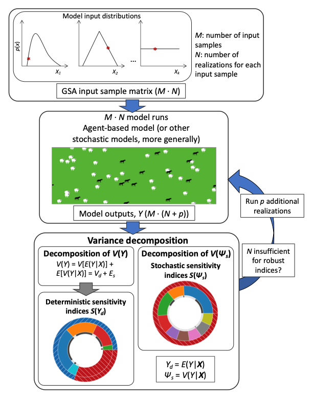
GSA quantifies how much changes in a model input are responsible for changes in model outputs by partitioning the total variance. If a model is simple enough, the importance of the inputs, the so-called sensitivity indices, \(S\), can be obtained analytically. For more complex models, like ABMs and most GSA applications, these values need to be estimated through Monte Carlo simulations (Saltelli 2002; Saltelli et al. 2010). These simulations are usually defined by pseudorandom samples of the input distributions that define a sample matrix of size \(M = (k + 2) \cdot L\) (for a conventional GSA, direct and total-order effects), where \(k\) is the number of model inputs \(\textbf{X} = \{X_{1}, X_{1}, \dots, X_{k}\}\), and \(L\) is the Monte Carlo sampling intensity. To account for model intrinsic stochasticity, \(N\) model realizations are generated for a given input sample, totaling \(M \cdot N\) realizations for the proposed GSA. The total output variance across the \(M \cdot N\) realizations, \(V(Y)\), can be decomposed into two components:
| \[ V(Y) = V[E(Y|\textbf{X})] + E[V(Y|\textbf{X})] = V(Y_{d}) + E(\Psi_{s}) = V_{d} + E_{s}\] | \[(1)\] |
The first component \(V_{d}\) can be further decomposed into:
| \[ V_{d} = V[E(Y_{d}\vee X_i)] + E[V(Y_{d} \vee X_i)]\] | \[(2)\] |
| \[ V_{d} = \sum_{i}V_{i}(Y_{d}) + \sum_{\{i,j\}}V_{i,j}(Y_{d}) + \sum_{\{i,j,l\}}V_{i,j,l}(Y_{d}) + \dots + \sum_{\{i,j,l,\dots, k\}}V_{i,j,l,\dots, k}(Y_{d})\] | \[(3)\] |
| \[ S_{\textbf{J}}(Y_{d}) = \frac{V_{\textbf{J}}(Y_{d})}{V(Y)}\] | \[(4)\] |
| \[ S_{T_{i}}(Y_{d}) = \frac{V(Y) - E_{S} - V[E[Y_{d}|\textbf{X}_{\sim i}]]}{V(Y)} = \frac{V_{d} - V[E[Y_{d}|\textbf{X}_{\sim{i}}]]}{V(Y)} = \frac{E[V[Y_{d}|\textbf{X}_{\sim i}]]}{V(Y)} \\ = S_{i}(Y_{d}) + S_{i,j}(Y_{d}) + \dots + S_{i, j \dots, k}(Y_{d})\] | \[(5)\] |
To investigate the stochastic uncertainty \(E_{s}\) (Equation 1), we can treat the variance across model realizations associated with a given input sample, \(\Psi_{s} = V(Y|X)\), as an output of the model (much like parameters of a random variable are considered constant). If the number of realizations is large enough we can estimate the conditional variances \((V_{i}(\Psi_{s}), V_{i,j}(\Psi_{s}), \dots)\) and, similarly to \(V_{d}\), further decompose the variance \(V(\Psi_{s})\) with the stochastic sensitivity indices \(S_{J}(\Psi_{s})\) and \(S_{T_{i}}(\Psi_{s})\) defined as:
| \[ S_{\textbf{J}} = \frac{V_{\textbf{J}}(\Psi_{s})}{V(\Psi_{s})}\] | \[(6)\] |
| \[ S_{T_{i}}(\Psi_{s}) = 1 - \frac{V[E[\Psi_{s}|\textbf{X}_{\sim i}]]}{V(\Psi_{s})} = \frac{E[V[\Psi_{s}|\textbf{X}_{\sim i}]]}{V(\Psi_{s})}\] | \[(7)\] |
These stochastic sensitivity indices identify what inputs contribute the most to the variance of the realizations around the expected output values. Notice that the stochastic sensitivity indices are referred to the variance around the expected output values for each input sample, \(V(\Psi_{s})\), and not to the total output variance, \(V(Y)\), as before.
Proposed GSA ABM evaluation approach
To illustrate Approach IV, we investigate how sensitive ABM outputs and their stochastic uncertainty are to inputs after the outputs have reached the steady state (in the stochastic sense). Approach IV (Figure 1) starts with a sample matrix with \(M\) input samples drawn from the specified input distribution (Saltelli et al. 2010). At first, \(N\) realizations are generated for each input sample in the sample matrix to obtain robust sensitivity indices (i.e., sensitivity indices are robust if the improvement in their estimates by increasing \(N\) is negligible) and estimate \(V_{d}\) and \(S(\Psi_{s})\). Then, the total output variance, \(V(Y)\), of the \(M \cdot N\) model runs (realizations) is decomposed in two steps, as described in the preceding section. From this decomposition deterministic and stochastic sensitivity indices are obtained, as well as the fractions of total variance due to deterministic \(V_{d}\) and stochastic (\(E_{s}\)) uncertainty. Because, the estimation of the stochastic sensitivity indices requires more realizations, \(N\) can start from a relatively small number (\(N = 10\)) and can be increased later, if the sensitivity indices are not robust and the stochastic uncertainty, fraction of variance (Equation 1) allocated to stochastic uncertainty (\(E_{s}\)), is high. The robustness of the sensitivity indices to bias due to the stochastic uncertainty for a certain \(N\) can be assessed through bootstrap resampling the realizations (\(N\)) and re-estimation of the sensitivity indices. If \(N\) realizations are insufficient to obtain robust estimates of the sensitivity indices, \(N\) can be increased by running \(p\) additional realizations of the GSA sample matrix.
Testing the approaches on two case studies
We make use of the GSA-benchmark Ishigami function (Homma & Saltelli 1996) with additive noise to compare the different estimates of \(S(Y_{d})\) between the Approaches I, II and IV. Then, we extend the analysis and cross-approach comparison to a proof-of-concept human migration ABM (Oh et al. 2022). In our analysis of the ABM, we estimated both \(S(Y_{d})\) and \(S(\Psi_{s})\). The motivation to use two study cases is that while in the Ishigami function the stochasticity (i.e., the additive noise) is independent of the model inputs, in the ABM the stochasticity depends on the ABM inputs. Hence, only in the case of the ABM we study the decomposition of the stochastic uncertainty. This is identified and quantified by the Approach IV.
We used the Python library “SALib” (Herman & Usher 2017) to generate sample matrices and estimate sensitivity indices.
Ishigami function
The Ishigami function (Homma & Saltelli 1996) has three inputs whose distributions are \(X_{i} \sim U[-\pi, \pi]\). We introduce additive noise, \(\epsilon \sim N(0, 2)\), to the function to turn it into a stochastic function. The sampling intensity, \(L\), was fixed to 1024 for all three studied approaches. For Approaches II and IV, 10 realizations were run.
| \[ Y = \sin(X_{1}) + 7 \sin(X_{2})^{2} + 0.1X_{3}^{4} \sin(X_{1}) + \epsilon\] | \[(7)\] |
The fraction of variance introduced by the noise, \(S_{\epsilon}\), is estimated as its variance (\(V_{\epsilon}\)), which equals the stochastic component over, \(E_{s}\), over the total variance, \(V(Y)\):
| \[ S_{\epsilon} = \frac{V_{\epsilon}}{V(Y)} = \frac{E_{s}}{V(Y)}\] | \[(8)\] |
The analytical solutions for the sensitivity indices are included in the supplementary materials.
Proof-of-concept human migration ABM
In the proof-of-concept human migration ABM (Oh et al. 2022), agents in five regions evaluate water availability, social ties, and distance (defined by 9 inputs) during their two-step “push-pull” migration decision-making process. In the first stage, agents decide whether to migrate or not, depending on the availability of resources and social ties. If migrating, they then choose where to go among other regions based on water availability, social ties, and distance. The model proposes three alternative factor configurations (model structures) that represent how agents weigh water availability and social ties in their decision-making processes. We started by analyzing the importance of the factor configuration selection before analyzing in detail the “ADD” factor configuration (in the “ADD” configuration, factors evaluated by agents to meet their requirements are substitutable) (Table 2), the most commonly used configuration. We took populations in five regions (population 1-5) at the last timestep as outputs to analyze the importance of factor configuration and socio-environmental inputs. The model is explained in more detail in the supplementary materials, and its NetLogo code can be found in the CoMSES repository (https://www.comses.net/codebase-release/43c48c8c-a654-4c64-94ef-f6a477c08702). The interested reader is referred to Oh et al. (2022) for more analysis and discussion.
Input distribution must be estimated from literature or data analysis. In the absence of detailed information about the distribution of the inputs, the uniform distribution is the most conservative, as an unimportant input in a uniform distribution will not be important in other distributions. The proof-of-concept ABM had input ranges in \(\pm 25\%\) from the base value (Table 2). To ensure result stability (e.g., multi-stable outputs in a realization), the kurtosis coefficient was calculated for the last 1000 timesteps.
For the GSA considering factor configuration as an input, the generated sample matrix (Saltelli et al. 2010) had size \(M = 24576\), with \(L = 2048\), and $k =$10 inputs. 20 realizations were generated for each input in the GSA input sample matrix. After fixing the factor configuration to “ADD”, the generated sample matrix (Saltelli et al. 2010) has size \(M = 22528\), with \(L = 2048\), and \(k = 9\) inputs. 150 realizations were run for each input sample to investigate the effect of \(N\) on the estimation of \(S(Y_{d})\) and \(S(\Psi_{s})\).
| Input | Base value | Distribution | Description |
|---|---|---|---|
| conf | ADD | ["ADD", "OR", "AND"] | Factor configuration determines how resources and social factors are weighted. "ADD": substitutability, "OR": adaptability, "AND": complementarity (see Oh et al. 2022.) |
| meanwater | 100 | \(U[75, 125]\) | Mean available water for the five regions |
| gradient | -10 | \(U[-12.5, -7.5]\) | Slope of linear decay in water availability as populations are further from the resource |
| bet11 | 4 | \(U[3, 5]\) | Weight of water availability in calculating push step migration |
| bet12 | 4 | \(U[3, 5]\) | Weight of social ties in calculating push step migration |
| alp1 | 0.3 | \(U[0.225, 0.375]\) | Probability change in push step due to water availability |
| alp2 | 0.3 | \(U[0.225, 0.375]\) | Probability change in push step due to social ties |
| bet21 | 4 | \(U[3, 5]\) | Weight of water availability in calculating pull step migration |
| bet22 | 4 | \(U[3, 5]\) | Weight of social ties in calculating pull step migration |
| bet23 | 4 | \(U[3, 5]\) | Weight of distance in calculating pull step migration |
Results and Discussion
Study case I: Ishigami function
The comparison of the estimates of the sensitivity indices obtained from Approaches I, II and IV to the analytical solution of the Ishigami function with additive noise are presented in Table 3. Only Approach IV correctly identified part of \(V(Y)\) as stochastic, \(S_{\epsilon}\), while Approaches I and II treated the model as deterministic. Approach I confused the stochastic uncertainty for interactions of the inputs (\(S_{1, 2,3}\)), leading to the overestimations of all \(S_{T_{i}}\). GSA results following Approach II were not representative of \(Y\) but of \(E[Y|\textbf{X}]\) which resulted in an overestimation of all the sensitivity indices. Approach IV correctly estimated input importance. The simulation costs of Approaches II and IV were the same because we did not decompose the stochasticity of the Ishigami function. As this stochasticity is additive noise and hence, independent of the model inputs.
| Approach I | Approach II | Approach IV | Analytical | |
|---|---|---|---|---|
| \(S_1(Y_d)\) | 0.213 | 0.315 | 0.245 | 0.244 |
| \(S_2(Y_d)\) | 0.362 | 0.440 | 0.342 | 0.343 |
| \(S_3(Y_d)\) | 0.007 | 0.009 | 0.007 | 0 |
| \(S_{1,2}(Y_d)\) | 0.012 | 0.011 | 0.008 | 0 |
| \(S_{1,3}(Y_d)\) | 0.203 | 0.239 | 0.186 | 0.189 |
| \(S_{2,3}(Y_d)\) | -0.059 | 0 | 0 | 0 |
| \(S_{1,2,3}(Y_d)^{*}\) | 0.213 | 0.001 | 0.001 | 0 |
| \(S_{T_{1}}(Y_d)\) | 0.633 | 0.555 | 0.432 | 0.433 |
| \(S_{T_{2}}(Y_d)\) | 0.565 | 0.441 | 0.343 | 0.343 |
| \(S_{T_{3}}(Y_d)\) | 0.389 | 0.245 | 0.191 | 0.189 |
| \(S_\varepsilon\) | 0 | 0 | 0.222 | 0.224 |
| Cost (realizations)\(^{**}\) | 8192 | 81920 | 81920 | - |
Study case II: proof-of-concept migration ABM
Effect of factor configuration
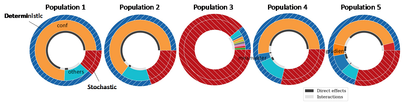
In the analysis of the ABM, we first determined the model sensitivity of all inputs, including factor configuration, for the deterministic uncertainty (Figure 2, Table 4). Here, we studied how important the choice between alternative model structure is. The outer ring represents the fraction of the variance assigned to \(V_{d}\) (deterministic–hashed blue colored) and \(E_{S}\) (stochastic–hashed red colored). The middle ring shows the fraction assigned to the total-order effect of each input (i.e., \(S_{T_{i}}(Y_{d})\)). The inner ring shows the portion of \(S_{T_{i}}(Y_{d})\) of each input caused by direct effects and interactions among inputs. \(V_{d}/V(Y)\) was 0.87, 0.80, 0.11, 0.71 and 0.71 for populations 1 to 5. Hence, population 3 is mostly random and dominated by stochastic uncertainty. The direct effects of factor configuration, ‘conf’, were found to explain most of the total variance for all populations except population 3: how the factors are weighted in the agent’s decision process is more important that the values of the model inputs (at least for the input ranges used in this analysis). Hence, in this study case, deciding between the alternative model configurations should be prioritized over studying the effects of the other inputs, as these only explained small fractions of the total variance.
| Population 1 | Population 2 | Population 3 | Population 4 | Population 5 | ||||||
|---|---|---|---|---|---|---|---|---|---|---|
| Input | \(S_i(Y_d)\) | \(S_{T_i}(Y_d)\) | \(S_i(Y_d)\) | \(S_{T_i}(Y_d)\) | \(S_i(Y_d)\) | \(S_{T_i}(Y_d)\) | \(S_i(Y_d)\) | \(S_{T_i}(Y_d)\) | \(S_i(Y_d)\) | \(S_{T_i}(Y_d)\) |
| conf | 0.81 | 0.85 | 0.72 | 0.77 | 0.01 | 0.08 | 0.62 | 0.69 | 0.47 | 0.58 |
| meanwater | 0.01 | 0.04 | 0.01 | 0.03 | 0.01 | 0.06 | 0.01 | 0.06 | 0.06 | 0.13 |
| gradient | 0.01 | 0.02 | 0.01 | 0.02 | 0.00 | 0.05 | 0.01 | 0.03 | 0.06 | 0.09 |
| bet11 | 0.00 | 0.02 | 0.00 | 0.02 | 0.00 | 0.06 | 0.00 | 0.03 | 0.00 | 0.03 |
| bet12 | 0.00 | 0.03 | 0.00 | 0.03 | 0.00 | 0.05 | 0.01 | 0.04 | 0.01 | 0.06 |
| alp1 | 0.00 | 0.01 | 0.00 | 0.01 | 0.00 | 0.05 | 0.00 | 0.01 | 0.00 | 0.02 |
| alp2 | 0.00 | 0.01 | 0.00 | 0.02 | 0.00 | 0.05 | 0.00 | 0.02 | 0.00 | 0.02 |
| bet21 | 0.00 | 0.01 | 0.00 | 0.01 | 0.00 | 0.05 | 0.00 | 0.01 | 0.00 | 0.01 |
| bet22 | 0.00 | 0.01 | 0.00 | 0.02 | 0.01 | 0.07 | 0.00 | 0.02 | 0.00 | 0.02 |
| bet23 | 0.00 | 0.01 | 0.00 | 0.01 | 0.00 | 0.05 | 0.01 | 0.02 | 0.00 | 0.02 |
| Sum | 0.84 | 1.01 | 0.74 | 0.96 | 0.03 | 0.57 | 0.67 | 0.93 | 0.60 | 0.97 |
Estimation of \(S(Y_{d})\) and \(S(\Psi_{s})\) when factor configuration is fixed to “ADD”
We continued the model analysis with fixing factor configuration to “ADD” and investigating through resampling with replacement the effect of increasing the number of model realizations \(N\) (Figure 3). For the sake of simplicity, only the GSA results of some populations are presented in this section (figures of the remaining populations are included in the supplementary materials). Different from the Ishigami function with additive noise, the stochastic uncertainty of stochastic ABMs (and stochastic models, in general) is affected by the model inputs. The decomposition of \(V(\Psi_{s})\) allows us to estimate the importance of the inputs for the stochastic uncertainty, \(S(\Psi_{s})\). As \(N\) increased, the uncertainty of the \(S(Y_{d})\) and \(S(\Psi_{s})\) decreased. This is the only trend observed for \(S_{i}(Y_{d})\) (Figure 3a and 3b). In the case of the \(S_{T_{i}}(Y_{d})\), false interactions were found for low values of \(N\) that disappeared as \(N\) increased (\(N \geq 10\)), identified by notable changes in \(S_{T_{i}}(Y_{d})\) (Figure 3c and 3d). These false interactions stemmed from stochastic uncertainty as explained in the Ishigami study case. In the case of \(S_{T_{i}}(\Psi_{s})\), the results showed that input importance can be ranked for a high enough value of \(N\) (e.g., \(N > 25\)) (Figure 3e and 3f), when important and unimportant inputs separate. Greater values of \(N\) would be needed for more accurate quantifications. However, ranking input importance is sufficient for factor prioritization (a common GSA objective).
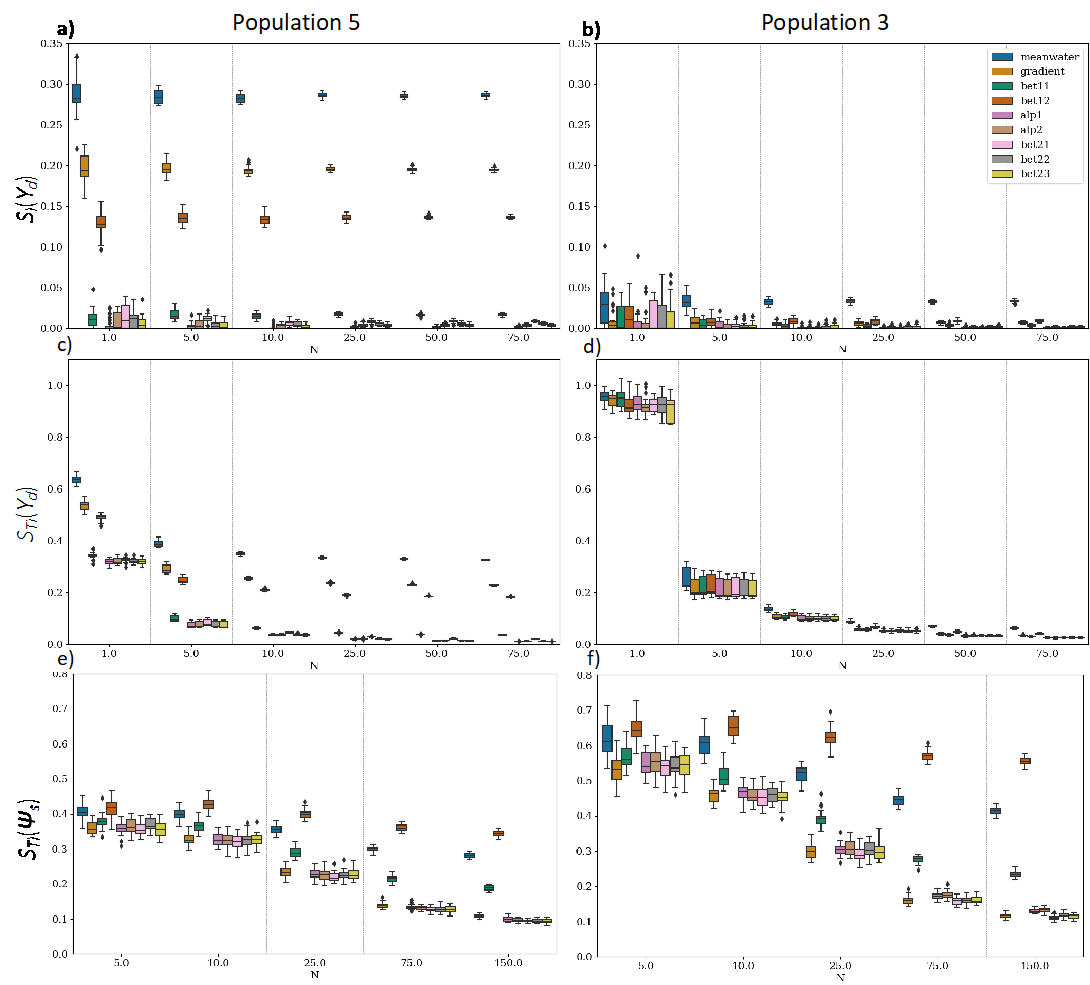
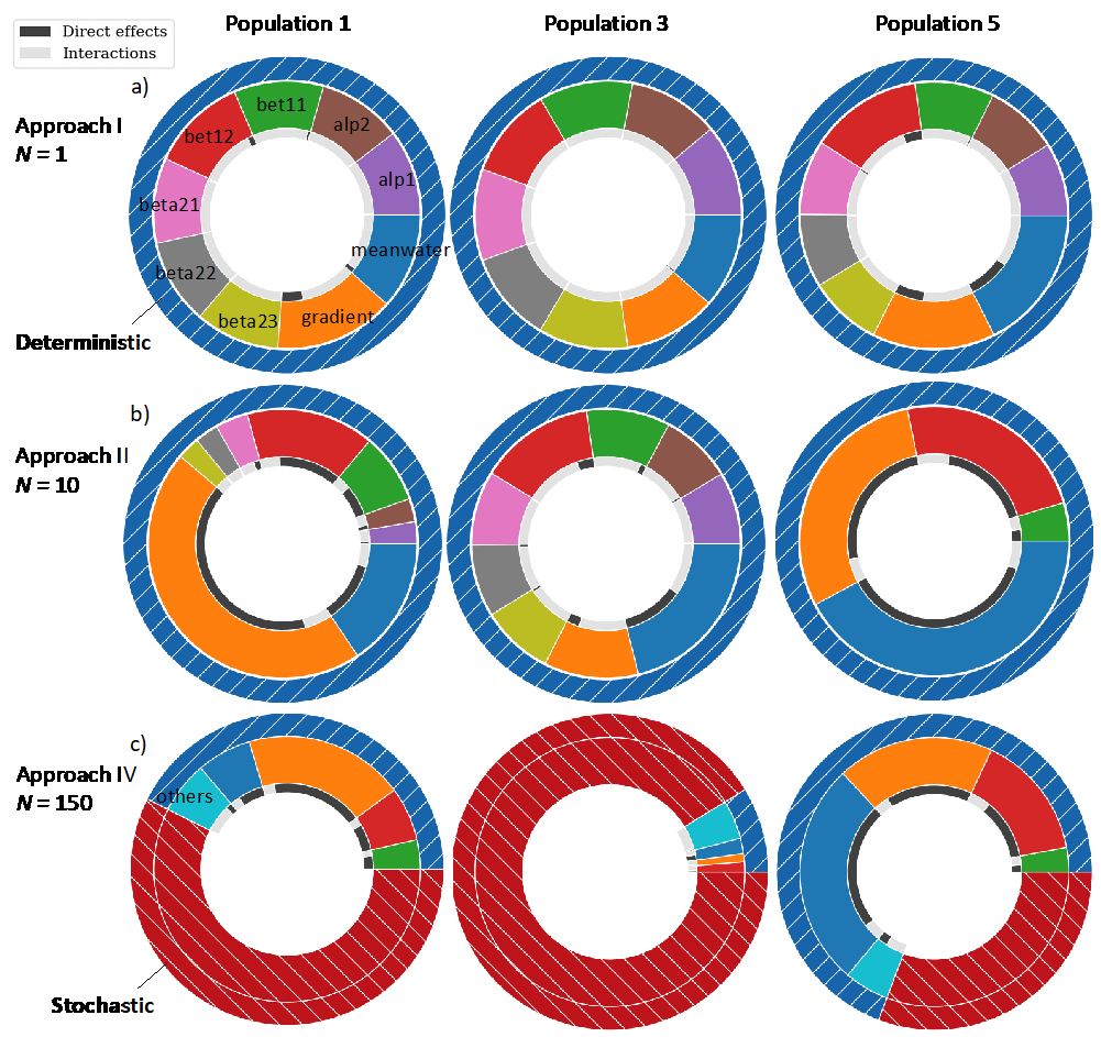
Figure 4 presents input importance for the deterministic and stochastic uncertainties for population 1, 3, and 5 following Approach IV that allowed for the interpretation of input importance through \(S(Y_{d})\) and \(S(\Psi_{s})\). In this ABM, a high fraction of the output variance was caused by stochastic uncertainty. This fraction was 0.59, 0.52, 0.93, 0.81 and 0.31 for populations 1 to 5. As in Figure 2, Population 3 was mostly random after fixing the factor configuration to “ADD”. This was likely due to its location, having the lowest average distance to each region, being likely that agents move to this region when distance is the most determining criterion for migration.
For the deterministic uncertainty of population 1, the most important inputs were “gradient”, “meanwater”, “bet12” and “bet11” that explained 22%, 7%, 7% and 3% of the total variance, respectively (Figure 4a, Table 5). For population 3, inputs had almost no impact on the deterministic uncertainty. In the case of population 5, the \(S_{T_{i}}(Y_{d})\) of “meanwater”, “gradient” and “bet12” explained 28%, 19% and 15% of the total variance, respectively. Population 1 and 5 shared the three most important inputs for their deterministic uncertainties that were mainly affected by environmental factors – average water availability (“meanwater”) and equal/inequal water allocations across five regions (“gradient”) – and social ties when deciding whether to migrate or not (“bet12”). Other inputs were responsible for a small fraction of the changes in the outputs. Additionally, most of the deterministic uncertainty of population 1 and 5 was explained by direct effects, \(S_{i}(Y_{d})\).
In the case of the stochastic uncertainty (Figure 4b, Table 5), “bet12”, “meanwater” and “bet11” were the most important inputs for population 1, explaining 29%, 23% and 14% of \(V(\Psi_{s})\), respectively. Notice that “gradient”, previously identified as the most important for the deterministic uncertainty of this output, was not as important for the stochastic uncertainty. And “bet11”, the weight agents give to water availability when deciding whether to migrate, was important. For population 3, “bet12”, “meanwater” and “bet11” were the most important inputs, explaining 35%, 25% and 13% of \(V(\Psi_{s})\), respectively. In the case of population 5, the most important inputs were “meanwater” and “bet11” with 29% and 15% of \(V(\Psi_{s})\), respectively. Interestingly, “bet12”, the weight of social ties when agents evaluate their need to migrate, was the most important input for the stochastic uncertainty of both population 1 and 3, but not for population 5. The combined information on the deterministic and stochastic sensitivity indices gave additional insights into the uncertainty of population 3. It showed that changes in the inputs had negligible importance for the expected value of population 3 but its variance was very sensitive to changes in “bet12”. As population 3 has the lowest mean distance among regions, it is very affected by inputs that increase the likelihood of agent migration such as the weight of social ties in deciding whether to migrate (i.e., “bet12”).

| Population 1 | Population 2 | Population 3 | Population 4 | Population 5 | ||||||
| Input | \(S_{i}(Y_{d})\) | \(S_{T_{i}}(Y_{d})\) | \(S_{i}(Y_{d})\) | \(S_{T_{i}}(Y_{d})\) | \(S_{i}(Y_{d})\) | \(S_{T_{i}}(Y_{d})\) | \(S_{i}(Y_{d})\) | \(S_{T_{i}}(Y_{d})\) | \(S_{i}(Y_{d})\) | \(S_{T_{i}}(Y_{d})\) |
| meanwater | 0.06 | 0.08 | 0.17 | 0.19 | 0.03 | 0.04 | 0.00 | 0.04 | 0.28 | 0.32 |
| gradient | 0.24 | 0.25 | 0.09 | 0.10 | 0.01 | 0.01 | 0.03 | 0.06 | 0.19 | 0.22 |
| bet11 | 0.03 | 0.04 | 0.02 | 0.03 | 0.00 | 0.01 | 0.03 | 0.04 | 0.02 | 0.03 |
| bet12 | 0.07 | 0.08 | 0.17 | 0.18 | 0.01 | 0.02 | 0.07 | 0.13 | 0.13 | 0.18 |
| alp1 | 0.00 | 0.00 | 0.00 | 0.01 | 0.00 | 0.01 | 0.00 | 0.01 | 0.00 | 0.00 |
| alp2 | 0.00 | 0.00 | 0.00 | 0.01 | 0.00 | 0.01 | 0.00 | 0.01 | 0.00 | 0.01 |
| bet21 | 0.01 | 0.01 | 0.01 | 0.01 | 0.00 | 0.01 | 0.00 | 0.01 | 0.01 | 0.01 |
| bet22 | 0.00 | 0.01 | 0.00 | 0.01 | 0.00 | 0.01 | 0.00 | 0.01 | 0.00 | 0.01 |
| bet23 | 0.00 | 0.00 | 0.00 | 0.00 | 0.00 | 0.01 | 0.00 | 0.01 | 0.00 | 0.00 |
| Sum | 0.41 | 0.47 | 0.45 | 0.53 | 0.06 | 0.13 | 0.14 | 0.30 | 0.64 | 0.78 |
| Population 1 | Population 2 | Population 3 | Population 4 | Population 5 | ||||||
| Input | \(S_{i}(\Psi_{s})\) | \(S_{T_{i}}(\Psi_{s})\) | \(S_{i}(\Psi_{s})\) | \(S_{T_{i}}(\Psi_{s})\) | \(S_{i}(\Psi_{s})\) | \(S_{T_{i}}(\Psi_{s})\) | \(S_{i}(\Psi_{s})\) | \(S_{T_{i}}(\Psi_{s})\) | \(S_{i}(\Psi_{s})\) | \(S_{T_{i}}(\Psi_{s})\) |
| meanwater | 0.28 | 0.40 | 0.28 | 0.37 | 0.26 | 0.41 | 0.25 | 0.45 | 0.43 | 0.52 |
| gradient | 0.03 | 0.12 | 0.02 | 0.09 | 0.02 | 0.07 | 0.01 | 0.08 | 0.03 | 0.19 |
| bet11 | 0.13 | 0.25 | 0.14 | 0.20 | 0.12 | 0.21 | 0.10 | 0.21 | 0.19 | 0.27 |
| bet12 | 0.38 | 0.51 | 0.35 | 0.48 | 0.41 | 0.57 | 0.34 | 0.51 | 0.00 | 0.21 |
| alp1 | 0.01 | 0.10 | 0.02 | 0.08 | 0.01 | 0.09 | 0.00 | 0.07 | 0.00 | 0.12 |
| alp2 | 0.01 | 0.10 | 0.01 | 0.09 | 0.01 | 0.09 | 0.00 | 0.07 | 0.01 | 0.12 |
| bet21 | 0.00 | 0.09 | 0.00 | 0.07 | 0.00 | 0.06 | 0.00 | 0.06 | 0.00 | 0.11 |
| bet22 | 0.02 | 0.09 | 0.02 | 0.07 | 0.03 | 0.07 | 0.00 | 0.06 | 0.02 | 0.13 |
| bet23 | 0.02 | 0.09 | 0.01 | 0.07 | 0.01 | 0.07 | 0.00 | 0.04 | 0.00 | 0.10 |
| Sum | 0.88 | 1.76 | 0.84 | 1.53 | 0.86 | 1.65 | 0.71 | 1.54 | 0.68 | 1.76 |
Comparison of ABM sensitivity for Approaches I, II and IV
Approaches I, II and IV led to very different sensitivities of the ABM (Figure 5), these results support previous calls for improving ABM and GSA transparency (Grimm et al. 2006; Lorscheid et al. 2012; Müller et al. 2013; Razavi et al. 2021). Approach I overestimated interactions and therefore \(S_{T_{i}}(Y_{d})\), identifying the model as highly interactive with all inputs being equally important, due to high stochastic uncertainty (Figure 5a). Approach II did not quantify input importance for stochastic uncertainty: results were not representative of the model outputs but of the expected value of the model outputs (Figure 5b). Approach I and Approach II did not identify population 3 as highly random and incorrectly attribute the variance to inputs. Only Approach IV (Figure 5c) correctly captured these stochastic uncertainties, overcoming the limitations of the previous approaches.
Conclusions
We reviewed the interpretation of ABM sensitivity for the GSA approaches identified. Using two study cases, a non-linear stochastic function and a proof-of-concept human migration ABM, we compared the differences among them and our proposed GSA approach that improves the interpretation of GSA results of ABM and other stochastic models. The differences among the approaches are due to how they address the model’s stochastic uncertainty during the GSA and whether they quantify input importance on stochastic uncertainty. Applications proceeding as Approaches I or II do not consider the effects of inputs on the stochastic uncertainty as a driver of the model outcomes and may lead to model misinterpretation. Approach I identifies the model as highly interactive due to the lumping of deterministic and stochastic uncertainties. In Approach II \(S(Y_{d})\) the stochastic uncertainty of the \(V(Y)\) is mitigated and not studied. In contrast, the proposed approach, Approach IV, estimates \(S(Y_{d})\) and \(S(\Psi_{s})\) accurately and illustrates that input importance on the deterministic uncertainty may be negligible with respect to the total output variance for highly stochastic outputs. Current GSA applications to ABMs do not inform about stochastic uncertainty which has implications for model interpretability. Finally, the identification of the most important inputs for the stochastic uncertainty helps evaluating alternative model structures, assessing the effect of increasing model complexity (e.g., addition of more inputs, more uncertainty, new processes, etc.).
A potential limitation of the proposed analysis is its computational cost that may be unaffordable for highly complex and parametrized models. In this case, emulating the model behavior is an option (Marrel et al. 2012; Prowse et al. 2016). However, analyses following Approach II have the same computational cost for the estimation of \(S(Y_{d})\) as Approach IV, but they do not inform about the stochastic uncertainty. Future research should assess the estimation of \(S(\Psi_{s})\) through emulators to reduce the computational cost of the analysis. More generally, the proposed approach has the potential to improve the interpretability and transparency of GSA results for other complex stochastic models beyond ABMs.
Acknowledgments
This research was supported by the Army Research Office/Army Research Laboratory under award #W911NF1810267 (Multidisciplinary University Research Initiative) and by the USDA National Institute of Food and Agriculture (2016-67019-26855), USDA-NIFA Hatch projects 1024705 and 1024706. The views and conclusions contained in this document are those of the authors and should not be interpreted as representing the official policies either expressed or implied of the Army Research Office or the U.S. Government. Woi Sok Oh is also pleased to acknowledge the support of the Princeton University Dean for Research and High Meadows Environmental Institute.References
ALDEN, K., Read, M., Timmis, J., Andrews, P. S., Veiga-Fernandes, H., & Coles, M. (2013). Spartan: A comprehensive tool for understanding uncertainty in simulations of biological systems. PLoS Computational Biology, 9(2), e1002916. [doi:10.1371/journal.pcbi.1002916]
AYLLÓN, D., Railsback, S. F., Vincenzi, S., Groeneveld, J., Almodóvar, A., & Grimm, V. (2016). InSTREAM-Gen: Modelling eco-evolutionary dynamics of trout populations under anthropogenic environmental change. Ecological Modelling, 326, 36–53.
BONABEAU, E. (2002). Agent-based modeling: Methods and techniques for simulating human systems. Proceedings of the National Academy of Sciences, 99(3), 7280–7287. [doi:10.1073/pnas.082080899]
CAI, R., & Oppenheimer, M. (2013). An agent-based model of climate-induced agricultural labor migration. Agricultural & Applied Economics Association 2013 Annual Meeting, Washington, DC
CENEK, M., & Dahl, S. K. (2016). Geometry of behavioral spaces: A computational approach to analysis and understanding of agent based models and agent behaviors. Chaos, 26, 11. [doi:10.1063/1.4965982]
CHAO, D. L., Halloran, M. E., Obenchain, V. J., & Longini, I. M. (2010). FluTE, a publicly available stochastic influenza epidemic simulation model. PLoS Computational Biology, 6(1), e1000656. [doi:10.1371/journal.pcbi.1000656]
DOSI, G., Pereira, M. C., & Virgillito, M. E. (2018). On the robustness of the fat-tailed distribution of firm growth rates: A global sensitivity analysis. Journal of Economic Interaction and Coordination, 13(1), 173–193. [doi:10.1007/s11403-017-0193-4]
DUNHAM, J. B. (2005). An agent-Based spatially explicit epidemiological model in MASON. Journal of Artificial Societies and Social Simulation, 9(1), 3. https://www.jasss.org/9/1/3.html
ENTWISLE, B., Williams, N. E., Verdery, A. M., Rindfuss, R. R., Walsh, S. J., Malanson, G. P., Mucha, P. J., Frizzelle, B. G., McDaniel, P. M., Yao, X., Heumann, B. W., Prasartkul, P., Sawangdee, Y., & Jampaklay, A. (2016). Climate shocks and migration: An agent-based modeling approach. Population and Environment, 38(1), 47–71. [doi:10.1007/s11111-016-0254-y]
GRIMM, V., Berger, U., Bastiansen, F., Eliassen, S., Ginot, V., Giske, J., Goss-Custard, J., Grand, T., Heinz, S. K., Huse, G., Huth, A., Jepsen, J. U., JNørgensen, C., Mooij, W. M., Müller, B., Pe’er, G., Piou, C., Railsback, S. F., Robbins, A. M., Robbins, M. M., Rossmanith, E., Rüger, N., Strand, E., Souissi, S., Stillman, R. A., VabNø, R., Visser, U. & DeAngelis, D. L. (2006). A standard protocol for describing individual-based and agent-based models. Ecological Modelling, 198(1), 115–126. [doi:10.1016/j.ecolmodel.2006.04.023]
GRIMM, V., Revilla, E., Berger, U., Jeltsch, F., Mooij, W. M., Railsback, S. F., Thulke, H.-H., Weiner, J., Wiegand, T., & DeAngelis, D. L. (2005). Pattern-oriented modeling of agent-Based complex systems: Lessons from ecology. Science, 310(5750), 987–991. [doi:10.1126/science.1116681]
HERMAN, J., & Usher, W. (2017). SALib: An open-source Python library for sensitivity analysis. Journal of Open Source Software, 2(9), 2017. [doi:10.21105/joss.00097]
HOMMA, T., & Saltelli, A. (1996). Importance measures in global sensitivity analysis of nonlinear models. Reliability Engineering & System Safety, 52(1), 53–78. [doi:10.1016/0951-8320(96)00002-6]
KNIVETON, D., Smith, C., & Wood, S. (2011). Agent-based model simulations of future changes in migration flows for Burkina Faso. Global Environmental Change, 21, 34–40. [doi:10.1016/j.gloenvcha.2011.09.006]
LEE, J.-S., Filatova, T., Ligmann-Zielinska, A., Hassani-Mahmooei, B., Stonedahl, F., Lorscheid, I., Voinov, A., Polhill, J. G., Sun, Z., & Parker, D. C. (2015). The complexities of agent-Based modeling output analysis. Journal of Artificial Societies and Social Simulation, 18(4), 4. https://jasss.org/18/4/4.html [doi:10.18564/jasss.2897]
LIGMANN-ZIELINSKA, A., Liu, W., Kramer, D. B., Cheruvelil, K. S., Soranno, P. A., Jankowski, P., & Salap, S. (2014). Multiscale spatial sensitivity analysis for agent-based modelling of coupled landscape and aquatic systems. Proceedings - 7th International Congress on Environmental Modelling and Software: Bold Visions for Environmental Modeling, IEMSs 2014, 1, 572–579 [doi:10.1016/j.envsoft.2014.03.007]
LIGMANN-ZIELINSKA, A., Siebers, P. O., Maglioccia, N., Parker, D., Grimm, V., Du, E. J., Cenek, M., Radchuk, V. T., Arbab, N. N., Li, S., Berger, U., Paudel, R., Robinson, D. T., Jankowski, P., An, L., & Ye, X. (2020). “One size does not fit all”: A roadmap of purpose-driven mixed-method pathways for sensitivity analysis of agent-based models. Journal of Artificial Societies and Social Simulation, 23(1), 6. http://jasss.soc.surrey.ac.uk/23/1/6.html [doi:10.18564/jasss.4201]
LIGMANN-ZIELINSKA, A., & Sun, L. (2010). Applying time-dependent variance-based global sensitivity analysis to represent the dynamics of an agent-based model of land use change. International Journal of Geographical Information Science, 24(12), 1829–1850. [doi:10.1080/13658816.2010.490533]
LORSCHEID, I., Heine, B. O., & Meyer, M. (2012). Opening the “Black box” of simulations: Increased transparency and effective communication through the systematic design of experiments. Computational & Mathematical Organization Theory, 18(1), 22–62. [doi:10.1007/s10588-011-9097-3]
MACAL, C. M. (2016). Everything you need to know about agent-based modelling and simulation. Journal of Simulation, 10(2), 144–156. [doi:10.1057/jos.2016.7]
MAGLIOCCA, N., McConnell, V., & Walls, M. (2018). Integrating global sensitivity approaches to deconstruct spatial and temporal sensitivities of complex spatial agent-based models. Journal of Artificial Societies and Social Simulation, 21(1), 12. http://jasss.soc.surrey.ac.uk/21/1/12.html [doi:10.18564/jasss.3625]
MARREL, A., Iooss, B., Da Veiga, S., & Ribatet, M. (2012). Global sensitivity analysis of stochastic computer models with joint metamodels. Statistics and Computing, 22(3), 833–847. [doi:10.1007/s11222-011-9274-8]
MULLER, S., Muñoz-Carpena, R., & Kiker, G. (2010). Model relevance frameworks for exploring the complexity-Sensitivity-Uncertainty trilemma. NATO Science for Peace and Security Series C - Environmental Security, 39–65. [doi:10.1007/978-94-007-1770-1_4]
MÜLLER, B., Bohn, F., Dreßler, G., Groeneveld, J., Klassert, C., Martin, R., Schlüter, M., Schulze, J., Weise, H., & Schwarz, N. (2013). Describing human decisions in agent-based models - ODD+D, an extension of the ODD protocol. Environmental Modelling and Software, 48, 37–48.
OH, W. S., Carmona-Cabrero, A., Muñoz-Carpena, R., & Muneepeerakul, R. (2022). On the interplay among multiple factors: Effects of factor configuration in a proof-of-Concept migration agent-Based model. Journal of Artificial Societies and Social Simulation, 25(2), 7. https://www.jasss.org/25/2/7.html [doi:10.18564/jasss.4793]
PARKER, D. C., Manson, S. M., Janssen, M. A., Hoffmann, M. J., & Deadman, P. (2003). Multi-agent systems for the simulation of land-use and land-cover change: A review. Annals of the Association of American Geographers, 93(2), 314–337. [doi:10.1111/1467-8306.9302004]
PARRY, H. R., Topping, C. J., Kennedy, M. C., Boatman, N. D., & Murray, A. W. A. (2013). A Bayesian sensitivity analysis applied to an agent-based model of bird population response to landscape change. Environmental Modelling and Software, 45, 104–115. [doi:10.1016/j.envsoft.2012.08.006]
PRESTES García, A., & Rodríguez-Patón, A. (2016). Sensitivity analysis of repast computational ecology models with R/Repast. Ecology and Evolution, 6(24), 8811–8831. [doi:10.1002/ece3.2580]
PROWSE, T. A. A., Bradshaw, C. J. A., Delean, S., Cassey, P., Lacy, R. C., Wells, K., Aiello-Lammens, M. E., Akçakaya, H. R., & Brook, B. W. (2016). An efficient protocol for the global sensitivity analysis of stochastic ecological models. Ecosphere, 7(3), 1–17. [doi:10.1002/ecs2.1238]
RAILSBACK, S., & Grimm, V. (2011). Agent-Based and Individual-Based Modeling: A Practical Introduction. Princeton, NJ: Princeton University Press.
RAZAVI, S., Jakeman, A., Saltelli, A., Iooss, B., Borgonovo, E., Plischke, E., Lo, S., Iwanaga, T., Becker, W., Tarantola, S., Guillaume, J. H. A., Jakeman, J., Gupta, H., Melillo, N., Rabitti, G., Chabridon, V., Duan, Q., Sun, X., Kucherenko, S., & Maier, H. R. (2021). The future of sensitivity analysis : An essential discipline for systems modeling and policy support. Environmental Modeling and Software, 137, 104954. [doi:10.1016/j.envsoft.2020.104954]
RENARDY, M., Hult, C., Evans, S., Linderman, J. J., & Kirschner, D. E. (2019). Global sensitivity analysis of biological multiscale models. Current Opinion in Biomedical Engineering, 11, 109–116. [doi:10.1016/j.cobme.2019.09.012]
ROCHE, B., Drake, J. M., & Rohani, P. (2011). An agent-Based model to study the epidemiological and evolutionary dynamics of Influenza viruses. BMC Bioinformatics, 12(1), 87. [doi:10.1186/1471-2105-12-87]
SALTELLI, A. (2002). Making best use of model evaluations to compute sensitivity indices. Computer Physics Communications, 145(2), 280–297. [doi:10.1016/s0010-4655(02)00280-1]
SALTELLI, A., Annoni, P., Azzini, I., Campolongo, F., Ratto, M., & Tarantola, S. (2010). Variance based sensitivity analysis of model output. Design and estimator for the total sensitivity index. Computer Physics Communications, 181(2), 259–270. [doi:10.1016/j.cpc.2009.09.018]
SALTELLI, A., Ratto, M., Andres, T., Campolongo, F., Cariboni, J., Gatelli, D., Saisana, M., & Tarantola, S. (2008). Global Sensitivity Analysis: The Primer. Hoboken, NJ: John Wiley & Sons. [doi:10.1002/9780470725184]
SALTELLI, A., Tarantola, S., Campolongo, F., & Ratto, M. (2004). Sensitivity Analysis in Practice: A Guide to Assessing Scientific Models. Hoboken, NJ: Wiley Online Library. [doi:10.1002/0470870958]
SOBOL, I. M. (1993). Sensitivity estimates for nonlinear mathematical models. Math. Model and Comput. Exp., 9(4), 407–414.
TEN Broeke, G., van Voorn, G., & LigTENberg, A. (2016). Which sensitivity analysis method should I use for my agent-based model? Journal of Artificial Societies and Social Simulation, 19(1), 5. https://jasss.org/19/1/5.html [doi:10.18564/jasss.2857]
THIELE, J. C., Kurth, W., & Grimm, V. (2014). Facilitating parameter estimation and sensitivity analysis of agent-Based models: A cookbook using netlogo and “R”. Journal of Artificial Societies and Social Simulation, 17(3), 11. https://jasss.org/17/3/11.html [doi:10.18564/jasss.2503]
TOPPING, C. J., Høye, T. T., & Olesen, C. R. (2010). Opening the black box - Development, testing and documentation of a mechanistically rich agent-based model. Ecological Modelling, 221(2), 245–255. [doi:10.1016/j.ecolmodel.2009.09.014]
WALDROP, M. M. (2018). Free agents. Science, 360(6385), 144–147. [doi:10.1126/science.360.6385.144]
WALKER, W. E., Harremoës, P., Rotmans, J., Van Der Sluijs, J. P., Van Asselt, M. B. A., Janssen, P., & von Krauss, M. P. (2003). Defining uncertainty: A conceptual basis for uncertainty management in model-based decision support. Integrated Assessment, 4(1), 5–17. [doi:10.1076/iaij.4.1.5.16466]
WANG, Z., Bordas, V., & Deisboeck, T. S. (2011). Identification of critical molecular components in a multiscale cancer model based on the integration of Monte Carlo, resampling, and ANOVA. Frontiers in Physiology, 2, 1–10. [doi:10.3389/fphys.2011.00035]
WANG, Z., Deisboeck, T. S., & Cristini, V. (2014). Development of a sampling-based global sensitivity analysis workflow for multiscale computational cancer models. IET Systems Biology, 8(5), 191–197. [doi:10.1049/iet-syb.2013.0026]
WIEGAND, T., Revilla, E., & Knauer, F. (2004). Dealing with uncertainty in spatially explicit population models. Biodiversity and Conservation, 13, 53–78. [doi:10.1023/b:bioc.0000004313.86836.ab]
WILENSKY, U. (1997). NetLogo wolf sheep predation model. Center for Connected Learning and Computer-Based Modeling, Northwestern University, Evanston, IL. Available at: http://ccl.northwestern.edu/netlogo/models/WolfSheepPredation