Schwartz Human Values and the Economic Performance

, ,
and
aCracow University of Economics, Poland; bDepartment of Social Psychology and Personality, SWPS University of Social Sciences and Humanities, Poland; cDecision Analysis and Support Unit, SGH Warsaw School of Economics, Poland
Journal of Artificial
Societies and Social Simulation 27 (1) 2![]()
<https://www.jasss.org/27/1/2.html>
DOI: 10.18564/jasss.5023
Received: 03-Jul-2022 Accepted: 06-May-2023 Published: 31-Jan-2024
Abstract
In the literature, human values are defined as desirable, trans-situational goals serving as guiding principles in people's lives. Schwartz introduced the concept of ten different values that are grouped into four higher order values: openness to change, conservation, self-transcendence, and self-enhancement. Some of the Schwartz values will underlie acting for one's own good, the others for the good of the community. The collective output of the community will depend on these two types of actions and the relations between them. Acting for the benefit of others may, yet does not have to, increase the total benefit for the community, even when it leads to less benefit to the self. In this paper we provide an analogy for the mechanisms underlying the relation between Schwartz values and economic output. The observed economic output is a result of the behaviour of many heterogeneous agents interacting with each other. The main problem is to verify whether and how the differences in the distributions of Schwartz values in a given community may influence its collective economic output. We classify Schwartz values into two different groups, based on the different effects these values may have on the observed collective output. A higher importance of self-enhancement (power, achievement, and hedonism) and conservation (security, tradition, and conformity) increases working time in the public sector and the public goods return, while simultaneously lowering working time in the private sector and the private goods return. The values of openness to change (stimulation and self-direction) and self-transcendence (universalism and benevolence) have the opposite effect.Introduction
The goal of this paper is to provide the analogy, in the sense defined by Edmonds et al. (2019), as to how different Schwartz values influence the collective output of a society, as measured across three distinct dimensions: public goods provided, private goods provided and leisure time. European societies differ in their distribution of values and this affects their economic performance (Weckroth & Kemppainen 2016). As an example, the importance of power and achievement is higher in Central and Eastern Europe (CEE) than in Western Europe. A similar phenomenon may also be observed for different regions in the same country. For example, the importance of power and achievement is significantly higher in the London region than in the rest of the UK (Weckroth & Kemppainen 2016).
Empirical studies show that societies that are characterised by higher levels of economic performance (GDP per capita) have higher levels of hedonism, stimulation, self-direction, benevolence and universalism, and lower levels of conformity, power, security and achievement (Schwartz 2004; Schwartz & Bardi 2001). Empirical evidence shows that after the attainment of a certain level of economic performance (in terms of GDP per capita) the correlation between economic performance and achievement decreases, whereas the correlation rises between economic performance and the values of self-direction, hedonism and stimulation (Schwartz & Bardi 2001). All these conclusions are based mainly on empirical analysis of the macroeconomic data. These are observational studies that do not allow for causal conclusions.
Another literature approach that aims to relate Schwartz values and economic behaviour is based on laboratory experiments, see Sagiv et al. (2011). Although such an approach allows the study of causal mechanisms, it does not take into account the complex interactions and relationships between economic agents and their behaviour as observed in real life. The laboratory settings are highly simplistic in comparison to real-life situations and the experiments typically concentrate on only one chosen mechanism. As a result, the context is neglected, which hampers our understanding of the emergent consequences (for society as a whole) of the observed causal relationships.
We offer a new insight to both trends in the literature by building a bridge between laboratory experiments and the collective output, which is usually a result of multiple interactions of many heterogeneous agents, by means of agent-based modelling. In this way we study the emergent macro-consequences of the causal relationships between values and individual agent choices. In particular, this allows us to verify whether these mechanisms lead to performance relationships observed for the whole population. Agent-based modelling is the methodology whereby one can study the emergent behaviour of the whole system itself, by taking into consideration the behaviours and interactions of many heterogeneous agents (Farmer & Foley 2009; Macal 2016).
We follow the concept of ten universal human values, introduced by Schwartz (1992) and the existing literature on the relation between Schwartz values and economic individual and collective output. Following microeconomic theory, we interpret the collective economic result as being threefold: public goods, private goods and leisure time. We model public goods provision with a classical linear public goods game (Cornes & Hartley 2007), while private goods provision is modelled with a classical trust game (Berg et al. 1995). The division into public goods, private goods and leisure time is a standard division present in economics (Mas-Colell et al. 1995) and thus we make use of it also. To the best of our knowledge, public goods, private goods and leisure time have not yet been investigated in the context of the Schwartz basic human values as measures of economic output.
In the paper we propose an agent-based model, in which the behaviour of the agents, and consequently the interactions between them in a public goods game and a trust game, depend on the Schwartz values. In the public goods game, multiple agents simultaneously choose how much – of their initial endowment of the total available working time – to contribute to a public good. The amount of public good provided and fully available to every agent depends on the total contributions of agents’ working time devoted to public good production. In the trust game, agents are matched in pairs and assigned either the role of investor or responder. The trust game is played sequentially. Firstly, the investor decides on the amount of working time to be invested with the responder. The amount of private good produced is a multiple (we use multiplication by a constant in the simulation) of the amount of working time originally invested in its production. Secondly, the responder decides the proportion of the final amount of private good produced to be returned to the investor and keeps the remainder. Both games are described in more detail in Sections 1.23 and 1.24. We use the results of experiments we have conducted to derive and parametrise how agents’ behaviour in these games depends on their Schwartz values. We provide analytical results for the simplified cases, where we analyse only two agents, taking each separately, first in a linear public goods game, and then in a trust game. The analytical solutions provide some initial intuition but do not allow us to capture the emergent consequences of many agents interacting in a community. Therefore, we used an agent-based approach to construct an analogy that better represents real-life economies. Adopting assumptions that are too simplistic in relation to reality may lead to deficiencies in models that are traceable analytically.
In particular, the following mechanisms are considered in the model. Firstly, many agents may participate in a public goods game at the same time. Secondly, agents may participate in both games at the same time, thus must decide how to share their effort. Thirdly, local interactions are considered by taking the geographical distance, neighbourhood and travelling cost into account. Fourth, the optimisation mechanism is implemented in the process of selecting the managers (working place) by the workers. Companies may be considered as hierarchical organisations, with a special role assigned to the managers (Male & Stocks 1989). Therefore, we consider two types of agents in our model: managers (further subdivided into public goods and private goods managers) and workers. Mintzberg (1973) distinguishes ten work roles of managers, which are divided into three groups: inter-personnel, informational and decisional. In order to capture this specificity in the model, we introduce managers into it. In our model, we refer to the leadership and resource allocation role of the managers, in particular. For both public goods and private goods, managers organise the production, which enables the transformation of working time (as invested by the workers) into produced goods. Additionally, private goods managers decide on the product allocation among themselves and the workers. In particular, they assume the role of the responder in the trust game. The role of an investor is assumed by the workers. Using agent-based modelling makes it possible to take all these four mechanisms simultaneously into account.
In the following paragraphs, we outline the main features of the Schwartz value theory. Values can be considered as desirable goals that serve individuals or social units as guiding principles in life (Schwartz 1994). While affecting cognitive processes (Weber 2017), they determine the attitudes of individuals and motivate them to undertake value-congruent behaviour. The behavioural outcome in turn depends on the subjective hierarchy of values that is derived from personal motivations, goals or beliefs (Črešnar & Nedelko 2020; Schwartz 1992). In general, values are reactions to three universal challenges that societies and individuals deal with: (1) the needs of individuals as biological organisms, (2) the problem of coordination of social interactions, (3) a requirement for the perennial existence of social groups (Schwartz 1994), so that values might originate from an organism, an interaction of a group, or a mixture of them (for instance, power stems from both the problem of coordination of social interactions and the perennial existence of social groups, while hedonism is rooted mainly in the organism).
Some values are related to the “self” which means the characteristics agents use to think of themselves (Rogers 1961). Therefore, “self” activation leads to the automatic activation of values (Hitlin 2003, 2008; Wojciszke 1986). Moreover, “self” related information is often processed quickly, suggesting automaticity in this case. Values central to a person’s sense of “self” are particularly motivating, and more likely to become active in a given situation (Verplanken & Holland 2002). It is also possible that in a certain social context more than one value will be activated. In such a case, the final motivational impulse constitutes a trade-off between them (Miles 2015). Values work as a system (trade-offs between different values) and as such they have an impact on an agent’s behaviour.
From a psychological perspective, values operate according to dual-process models (Miles 2015). There are two levels of cognition (Epstein et al. 1996): one is fast, effortless and relatively automatic, the other is slow and deliberative. Usually, people rely on automatic processes, with deliberative thought only activated occasionally, such as when people tackle a difficult situation or are in a specific situation that provokes deliberative processes (Evans 2008). When making decisions, they apply various mental tools relating to both rational reasoning (logic, statistics) or intuition (heuristics). Interestingly, using simple heuristics that save time and effort, as compared to complex analysis, may simultaneously improve the accuracy of judgments, despite disregarding some of the information (Gigerenzer & Gaissmaier 2011). In an uncertain world, both heuristics and other internal explanations of behaviour (e.g., perceptions, attitudes, values) are important components of the decision-making toolbox of an individual. Regardless of whether values operate automatically or deliberatively, they need to be activated to influence behaviour. Apart from “self” activation, abstract thinking, such as that concerning values or the meaning of action, leads to values activation also (Torelli & Kaikati 2009; Verplanken & Holland 2002).
Values are relatively stable during an individual’s lifetime (Bardi & Goodwin 2011). They are central to the self and serve important psychological functions, e.g., motivational and normative. It makes personal values especially resistant to change (Brewer 2015). However, changes in personal values are possible (Schwartz 2005; Schwartz 2012). This may be caused by various events experienced during the course of a lifetime or through self-chosen life-transitions (Bardi et al. 2014). Individuals are able to maintain a good value fit to various situations encountered in their lives, primarily through a selection of life settings that are congruent with their personal values (Bardi et al. 2014). To a much lesser extent, they achieve it by altering their personal values in order to make them fit to a life situation (Bardi et al. 2014). An example of such a value adaptation trigger could be the changes in macroeconomic conditions. Specifically, the phase of the business cycle in which people enter the job market is important for their values later in life (Duffy 2021; Elder 2018; Inglehart & Abramson 1994). If people enter the job market in times of economic crisis, inflation and unemployment (e.g., being forced to drop out of school and enter the job market, as happened during the Great Depression), they are likely to be more focused on materialistic values later in life than people entering the job market in more prosperous periods (Duffy 2021; Elder 2018). On the other hand, Inglehart’s predictions on transition toward post-materialist values assume that, in spite of shocks related to the business cycle, the intergenerational shifts from materialistic to post-materialist values will continue as long as societies reach a high level of existential security (Inglehart & Abramson 1994; Inglehart 2008). Kiley & Vaisey (2020) analysis of the panel data from the General Social Survey shows that values, similarly to attitudes or world views, remain stable from the time of early socialisation.
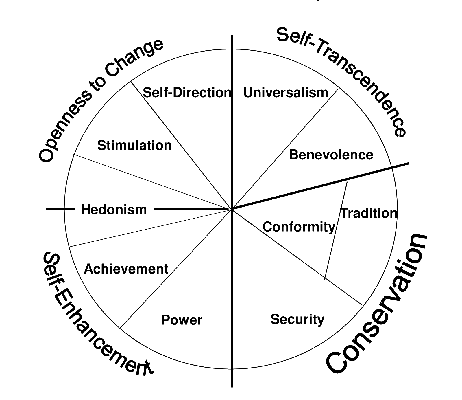
The Schwartz’ theory of human values has laid a reliable foundation for understanding the nature of values and operationalises its structure in the form of a circular continuum. The circular structure of basic human values, see Figure 1, which is the central proposition of this theory, implies that adjacent values are related to compatible motivations, whereas opposing ones are related to conflicting motivations. This circular structure of values reveals a high degree of robustness across cultures (Rudnev et al. 2018). Schwartz’s (Schwartz 1992; Schwartz 1994) typology of values consists of ten motivationally distinct types of values, arranged in opposing pairs: power vs. universalism; achievement vs. benevolence; hedonism and stimulation vs. conformity and tradition; self-direction vs. security. Table 1 summarises the main characteristics of particular values.
| Value | Description |
|---|---|
| Universalism | Understanding, appreciation, tolerance and protection for the welfare of all people and for nature. |
| Power | Social status and prestige, control or dominance over people and resources. |
| Benevolence | Preservation and enhancement of the welfare of people with whom one is in frequent personal contact. |
| Achievement | Personal success through demonstrating competence according to social standards. |
| Conformity | Restraint of actions, inclinations, and impulses likely to upset or harm others and violate social expectations or norms. |
| Stimulation | Excitement, novelty, and challenge in life. |
| Tradition | Respect, commitment and acceptance of the customs and ideas that traditional culture or religion provide the self. |
| Hedonism | Pleasure and sensuous gratification for oneself. |
| Security | Safety, harmony, and stability of society. |
| Self-direction | Independent thought and action, creating, exploring. |
These individual human values can further be grouped into higher dimensions, the so-called higher order value types (HOVs) which form the two bipolar dimensions: self-transcendence vs. self-enhancement and openness to change vs. conservation (Schwartz 1992). Schwartz acknowledges that he discovered potentially universal relations among value priorities (Schwartz 1994), for example, achievement values conflict with benevolence values. Indeed, this value typology has been confirmed in hundreds of samples taken from 82 nations, representing various age, cultural, religious and occupational groups (Schwartz 2012). This means that these groups recognize the same types of values and the trade-offs among them, not that they prize the same values (Schwartz 2012). Therefore, Schwartz’s value structure seems to be a general form of cultural content.1
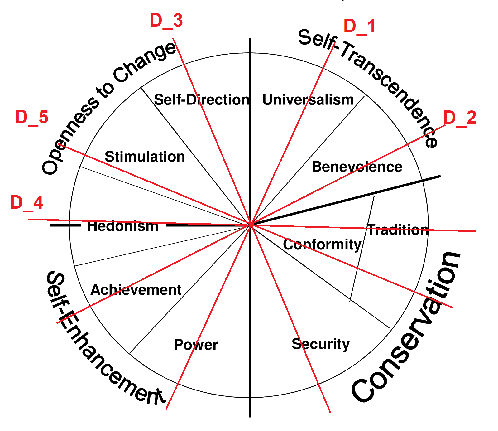
Values adjacent on the circular structure of Schwartz’s core values are highly positively correlated, while values on the opposite sides of the circular structure are highly negatively correlated (Schwartz 1994). This feature leads to methodological concerns related to multicollinearity (Perrinjaquet et al. 2007; Piurko et al. 2011; Schwartz et al. 2012). The preliminary analysis showed values of the Variance inflation Factor (VIF) above five, which is considered as a limit value for models with moderately and highly correlated variables (O’brien 2007).2. In order to address this, we construct \(D_i\) variables based on the original raw scores of the Schwartz values to overcome this problem. By doing this we propose a new method for the representation of ten Schwartz values as five dimensions (denoted \(D_1\) to \(D_5\) in the paper), which both retains the natural interpretation of the dimensions while making them more independent. The differences between opposite human values were obtained and five corresponding variables, \(D_1\) to \(D_5\), were constructed as follows: \(D_1\) = power – universalism, \(D_2\) = achievement – benevolence, \(D_3\) = self-direction – security, \(D_4\) = hedonism – (tradition + conformity)/2, \(D_5\) = stimulation – (tradition + conformity)/2. Variable \(D_1\) shows the difference between power and universalism, indicating how much an agent is focused on power at the expense of its opposing value – universalism. Other \(D_i\) variables may be interpreted in an analogous way. The \(D_i\) variables are graphically presented in Figure 2. In this approach, the highest value of VIF did not exceed three, which is an acceptable value. According to the structure of the Schwartz values presented in Figure 1, the conformity and tradition pair of Schwartz values are simultaneously opposite to both stimulation and hedonism. Such dependence was reflected in the construction of the confounded variables \(D_4\) and \(D_5\). An alternative approach would allow either \(D_4\) = hedonism – tradition and \(D_5\) = stimulation - conformity or \(D_4\) = hedonism – conformity and \(D_5\) = stimulation - tradition. Although such alternative approaches led to somehow better statistical properties (VIF values were on average smaller and did not exceed \(2.5\)), they are not completely consistent with the original results of Schwartz, who stated that such radial arrangement on the circle of the values – the conformity and tradition have a similar role – better corresponds to the results of empirical research (Schwartz 1992). Nevertheless, for other datasets, they may be a potential alternative to our approach. Such an approach deals better with multicollinearity issues than using the four higher order values defined by Schwartz: openness to change, conservation, self-transcendence and self-enhancement.
The most advanced programme of measuring values was introduced and conducted by Schwartz (1992), which was later extended by Schwartz and the European Social Survey (ESS) in a cross-national survey programme. The ESS is an academically driven survey founded in 2001 and run biennially by the ESS European Research Infrastructure Consortium, which aims at assembling, interpreting and disseminating rigorous and standardised data on the social condition of European citizens in different countries. These social conditions include, among others, human values, so each round of the survey provides updated information about evolutionary patterns in the value profiles of societies.
We propose a simulation that offers a novel way of thinking about how values as a system translate into collective output, measured across three dimensions: public goods provided, private goods provided and leisure time (Becker 1965; Chiappori 1988; Flores & Graves 2008; Konrad & Leininger 2011). Our intuitive understanding of this process is that within a society there is a series of trade-offs between individual decisions on time allocation among three factors: contributing to public goods production, contributing to private goods production and leisure time. The individual decisions governing how to allocate time are driven by the Schwartz values. The final outcome (in terms of public goods, private goods and leisure time) depends on the results of the series of these individual trade-offs and their societal combination. In our simulation we show which of these trade-offs and their combinations may lead to a better economic performance.
From an economic perspective, many empirical studies show that values and, more generally, culture, have an impact on economic performance (Alesina & Giuliano 2015) or subjective well-being (Sortheix & Schwartz 2017). Religious affiliations and ethnic background influence preferences for redistribution (Guiso et al. 2006), and cultural values affect development (Landes 2015). Similarly, values guide people in their economic activities and play a role in shaping their business relationships (Baur et al. 2016; Callaghan 2013; Castellani 2019; Gorgievski et al. 2011; Inglehart 2018; Ruf et al. 2021). For example, among the Schwartz values, high self-transcendence values and low conservation values may be associated with high national wealth and low income inequality (Tormos et al. 2017). However, the populations are not homogenous in terms of individual value endowments, and differences in value profiles within or across organizations, industries or countries are likely to translate into differences in their economic performance (Ariza-Montes et al. 2017; Cohen 2009; González-Rodrı́guez et al. 2016; Magun & Rudnev 2015; Torres et al. 2015).
Despite many political efforts to foster economic development, disparities between countries or societies continue to exist. Neoclassical attempts to explain long-term economic growth, indicating human resources, physical capital, and technological progress as proximate determinants of economic performance, have shown to offer limited success in unfolding the complexity of economic and social relationships that shape the growth patterns at both macro- and microeconomic level. More recent approaches in this field look beneath these proximate causes and put supplementary emphasis on non-economic sources of growth, such as institutions, geography, demography, political systems and their instabilities, government efficiency, and cultural or social drivers such as trust and cooperation (Acemoglu 2009; Aisen & Veiga 2013; Growiec et al. 2018; Kelley & Schmidt 2005; Lloyd & Lee 2018; Rodrik et al. 2004; Roos 2018), to name a few.
At the company level, business growth, profitability, and innovativeness are mostly guided by self‐enhancing value orientations, whereas softer success criteria of business owners (e.g., life-work balance) can be related to self-transcendent value orientations, such as benevolence and universalism (Gorgievski et al. 2011). According to Schwartz (1999), values are also related to different aspects of attitudes toward work, such as the importance of work in one’s life (called “work centrality”), societal norms about working (whether people are entitled or obliged to work) and the goals or rewards people expect from work the most. Values also affect competitive versus cooperative behaviour in social-dilemma games (Sagiv et al. 2011). In Sagiv’s first study, the contribution of participants correlated positively with the values of universalism and benevolence, and correlated negatively with power, achievement, and hedonism (Sagiv et al. 2011). In Sagiv’s second study, the contribution of participants correlated positively with emphasising benevolence over power values. (Sagiv et al. 2011) claim that there is a causal influence of values on action.3
Importantly, economic output can be considered in three separate dimensions, specified by public goods, private goods and leisure time. As microeconomic labour supply theory indicates, there is a labour-leisure trade-off that individuals face (Nicholson & Snyder 2012). As they value both income and leisure, their decision problem comes down to how to allocate available time between activities that provide income (work) and the unproductive ones which provide satisfaction (leisure). In such a case, the overall utility is a joint function of both categories. The trade-off reveals that under budget constraints individuals who prefer less work (more leisure) time earn less income than would otherwise be possible. Available working hours and wages determine the range of achievable combinations of income and leisure time, which constitutes the budget constraints.
The productive activities, in turn, can be distinguished between public or private good provision. In general, public goods are non-excludable and non-competing products or services that are beneficial and available to everyone without any direct payment obligation (e.g., clean air), or paid collectively through public taxation (e.g., the defence system). They are usually provided by governments and their consumption by one individual does not deter another individual’s ability to consume them. In contrast, private goods, which are purchased for personal consumption by the buyers are not available to other individuals, since their stocks are limited. Most private goods must be acquired for a cost, which is compensated by the buyer’s exclusive right to consume or use those goods. Unlike public goods, private goods usually allow the free rider problem to be avoided, i.e., a situation in which an individual uses a specific good without contributing to paying for it and avoiding possible consequences.
Both public and private good provision can be modelled in a game-theoretic framework. Public good games are used routinely by economists to examine inefficiencies in decentralised resource allocation mechanisms (Cornes & Hartley 2007). They allow the cooperation of heterogeneous individuals (affected by the pay-off functions or matching protocols) to be incorporated into repeated decision-making processes, and enable the transformation of individually differing preferences or beliefs into collective outcomes, and as a result they can provide micro-level explanations of macro-level regularities (Janssen & Ahn 2006; Ones & Putterman 2007). Nevertheless, the cooperation of individuals is prone to free-riding, and the potential fear of being exploited may induce selfish decisions. Therefore, the rational strategy of an individual player is to contribute nothing to the public good, regardless of what the other players do (Masel 2007; Ones & Putterman 2007).
In the standard linear public-good games, the game environment may be characterised by several parameters, including the number of players, the marginal per capita return, repetitions and the players’ initial endowments (e.g., tokens). During the game, agents secretly decide how much from a set fund to put into a common pool. Total contributions to the pool are then multiplied by a predefined factor (greater than 1 but less than the number of players) and distributed back equally in the form of a ‘public good’ pay-off to all game participants. Tokens not contributed for the common pool are kept by the players. The decision of an individual concerning how many tokens to contribute to the public good has a crucial impact on the collective output from the agent interactions. As experimental studies reveal, individuals usually contribute around half their available funds to the common pool, (Ledyard 1995) and the contribution level varies across players or between rounds, depending on group size, experiment duration and the marginal per capita return, among other factors (Janssen & Ahn 2006).
On the other hand, trust games, designed by Berg et al. (1995), are a popular measure of behavioural trust and trustworthiness in personal exchange. They emphasize the role of cooperative or competing strategies in generating anticipated future benefits at both the individual and collective level (Johnson & Mislin 2011; McCabe et al. 2003). In economic research, trust between people and willingness to engage in trustworthy behaviour in business relations have been indicated to positively affect the efficiency of firms (Dirks & Ferrin 2002) and national economic output (Algan & Cahuc 2013; Knack 2001; Knack & Keefer 1997). Therefore, integrating trust and game-theoretic logic into formal economic models allows for a more detailed picture of the role of the trustworthy or untrustworthy behaviours of market actors in shaping economic performance.4
In the standard two-person trust game, the anonymously paired individuals, endowed with an initial sum of money, interact together. The player who initiates the interaction, designates some amount of money to the second player. This amount can also be equal to zero. When tripled by the experimenter, the increased contribution is transferred to the second player, who follows the same procedure and makes their own choice on how much of the tripled money to give back to the counterparty. They are also allowed to send nothing. If the first player acted in an economically rational way, in the meaning of standard rational self-interest assumption, their payment to the second player should be equal to zero. However, as experimental studies reveal, such individually rational behaviour is more the exception than the rule among individuals (Berg et al. 1995; Brülhart & Usunier 2012).
The proposed agent-based model is detailed in a separate section, which follows the Introduction. In the remaining parts of the paper, we first present both data sets from the European Social Survey and experimental data and also the results of the econometric analysis. The analytical solutions of the simplified cases that provide some intuition about mechanisms implemented in the model are presented in the next section. We simulated different economic outputs for different distributions of the Schwartz values in the constructed set of the synthetic populations. The results of the statistical analysis of the simulation’s output and our conclusions are presented in the final two sections.
Agent Based Model
The purpose of the model is to provide an analogy for how the Schwartz values may influence the aggregated economic performance, as measured by: public goods provision, private goods provision and leisure time.
Agents are created and randomly located in a geographical space (we use the notion of Euclidean distance in our model). A separate agent population that is considered in the simulation has been created for Poland based on the results of the ESS9 survey, see section European Social Survey Data for the details). We consider a \([0,1] \times [0,1]\) grid and a torus topology.
The relevant agent characteristics are:
- spatial coordinates – each agent is characterised by two spatial coordinates \((x,y)\) corresponding to the geographic coordinates. These coordinates were sampled uniformly and independently for each agent.
- the Schwartz values - represented by the \(D_1\), \(D_2\), \(D_3\), \(D_4\), and \(D_5\) variables (see section European Social Survey Data for details).
- information concerning the employment status and occupation of an agent: a worker, a public good manager or a private good manager
- the maximal number of working hours
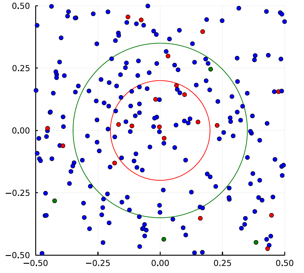
We use the concepts of geographical distance and travelling costs, taken from the field of economic geography (Krugman 1991), in order to account for the fact that participating in public or private goods games that are geographically remote may incur personal travelling costs for the agents. Moreover, we consider local interactions among agents by limiting the distance between managers and potential workers. In particular, each worker can see all the public goods managers that are located at a maximum distance of \(r_\textrm{publ}\) and all the private goods managers located at a distance no greater than \(r_\textrm{priv}\). We show the sample distribution of agents with distances marked for the agent in the grid centre in Figure 3.
In the initial simulation step, the agents randomly select both private and public goods managers (one each) from the managers, who are geographically closer than the maximum distance. If there is no manager that may be selected, then the agent will not invest their time in producing this kind of good.
Then, during each simulation step (we use 50 steps as this number is sufficient for the statistical analysis at the aggregated level of the entire agents population), three phases are considered for each agent:
- Phase 1 – Time allocation
- Phase 2 – Pay-off calculation
- Phase 3 – Decision regarding a potential change of managers
Time allocation
In this phase agents (workers) allocate their maximal number of working hours available to them among public goods production (with one of the previously selected public goods managers), private goods production (with one of the private goods managers) and potentially shirking. Thus, we interpret the total nominal number of working hours purely as an initial endowment that can be further divided between goods production and shirking. The latter variable is subsequently referred to in the text as leisure time.
The time allocation rules depend on the Schwartz values (among other factors) and are defined by the variables \(y_\textrm{publ}\) and \(y_\textrm{priv}\). Both variables represent the share of available working time invested in public and private good production, respectively. The rules are derived based on the data from the laboratory experiment and are described in more detail in Section 3 (Data). In particular, the results of the econometric analysis of the data from the linear public good game are used to specify the decision rule for \(y_\textrm{publ}\), and from the trust game for \(y_\textrm{priv}\).
The share of the time allocated to the provision of public goods \(y_\textrm{publ}\) depends on an agent’s Schwartz values, the difference between the agent’s own contribution and the average contribution of the other agents in the previous simulation step, and the number of times an agent invests with the same manager (\(\tau\)). The mathematical representation of this decision rule is given in Equation 15. The subscript ‘publ’ has been omitted here for the sake of readability.
| \[ y_i^{t+1}=\alpha_i + \beta_i^{+} \textrm{max} \left(y_i^t -y_{-i}^t ,0\right) + \beta_i^{-} \textrm{max} \left(y_{-i}^t -y_i^t, 0\right) + \gamma_i (\tau-1)\] | \[(1)\] |
In particular, we relate the absolute difference between the number of hours invested in a public good by an agent \(i\) to the total number of working hours of agent \(i\) in simulation step \(t\) (variable \(y_i^t\)). In a similar way, we relate the average value of the working hours for all other agents contributing to this public good to the total number of working hours of agent \(i\) (variable \(y_{-i}^t\)).6 For an agent \(i\), which is characterised by the Schwartz values \((D_1,D_2,D_3,D_4,D_5)\), the parameters’ values are calculated as follows:
\(\alpha_i = 0.689 - 0.044 D_1 - 0.004 D_2 + 0.013 D_3 - 0.008 D_4 + 0.026 D_5\) \(\beta_i^+ = 0.012 + 0.058 D_1 + 0.043 D_2 - 0.030 D_3 + 0.051 D_4 - 0.083 D_5\) \(\beta_i^- = 0.019 - 0.120 D_1 - 0.053 D_2 - 0.234 D_3 + 0.119 D_4 - 0.016 D_5\) \(\gamma_i = -0.019\)The share of time allocated to the provision of private goods \(y_\textrm{priv}\) depends on an agent’s Schwartz values, the percentage of the invested amount (after being multiplied by three) returned by the private good manager in the previous simulation step, and the number of times an agent invests with the same manager (\(\tau\)). The mathematical representation of this decision rule is given in Equation 27 The subscript ‘priv’ has been left out to aid readability. The variable \(z_j^t\) represents the percentage of the product produced by the agent (worker) \(i\) returned by the manager \(j\) in the simulation step \(t\).
| \[ y_i^{t+1}=\alpha_i + \beta_{1i} z_j^t + \beta_{2i} (\tau -1)\] | \[(2)\] |
For a given agent \(i\) the parameters are calculated in the following way:
\(\alpha_i = 0.477 + 0.001 D_1 + 0.012 D_2 - 0.003 D_3 + 0.012 D_4 - 0.004 D_5\) \(\beta_{1i} = 0.129\) \(\beta_{2i} = 0.01\)The number of working hours invested in public good production is calculated by multiplying the variable \(y_\textrm{publ}\) and the total number of working hours available \(n\). The number of working hours invested in a private good is calculated analogously. What remains is leisure time. The details are provided below in Equations 3, 4 and 5.
| \[ n_\textrm{publ} = n \times \frac{y_\textrm{publ}}{\textrm{max} \left(1, y_\textrm{publ} + y_\textrm{priv}\right)}\] | \[(3)\] |
| \[ n_\textrm{priv} = n \times \frac{y_\textrm{priv}}{\textrm{max} \left(1, y_\textrm{publ} + y_\textrm{priv}\right)}\] | \[(4)\] |
| \[ n_\textrm{leisure} = n - n_\textrm{publ} - n_\textrm{priv}\] | \[(5)\] |
Pay-off calculation
An agent’s (worker’s) pay-off from a public good depends on the total number of hours invested in the same public good (the same public goods manager) by the agent itself and the other agents, and the Euclidean distance between an agent and the selected public goods manager. Let us identify an agent with the superscript \(i\), a public goods manager with superscript \(j\), and define \(I\) as the set of all agents that invested in public goods manager \(j\). Then the pay-off of agent \(i\) is defined by Equation 6.
| \[ p^i = s_\textrm{publ} (1 - \gamma d(x_i,y_i,x_j,y_j)) \sum_{i \in I} n_\textrm{publ}^i\] | \[(6)\] |
The variables \(s_\textrm{publ}\) (public goods pay-off factor) and \(\gamma\) (travelling cost) are the simulation parameters. We define the distance \(d(x_i,y_i,x_j,y_j)\) on the torus in the manner defined in Equations 7 and 8.
| \[ d(x_i,y_i,x_j,y_j) = \sqrt{l(x_i - x_j)^2 + l(y_i - y_j)^2}\] | \[(7)\] |
| \[ l(x,y) = \min \left(\lvert x - y \rvert, 1 - \lvert x - y \rvert \right)\] | \[(8)\] |
The pay-off of the public goods manager \(j\) is calculated in the same way, but without taking the distance into account (see Equation 9).
| \[ p^j = s_\textrm{publ} \sum_{i \in I} n_\textrm{publ}^i\] | \[(9)\] |
An agent’s (worker’s) pay-off from a private good depends on the total number of hours invested in the private good (with the selected private goods manager), the share of the invested amount returned by the manager \(j\), \(z_j\), and the Euclidean distance between an agent and a private goods manager. The value of the variable \(z_j\) depends on the Schwartz values of the private goods manager, the ratio of number of hours invested by the workers with the private good manger \(n_\textrm{publ}\) to their total number of working hours available \(n\) (\(y_{\textrm{priv},i}^{t+1}\)) and the number of times a worker invests with the same manager (\(\tau\)). The mathematical representation of the decision rule is given in Equation 108.
| \[ z_j^{t+1}=\alpha_j + \beta_{1j} y_{\textrm{priv},i}^{t+1} + \beta_{2j} (\tau-1)\] | \[(10)\] |
For a given agent \(i\) the parameters are calculated, based on the Schwartz values of the private good manager, in the following way:
\(\alpha_j = 0.418 - 0.02 D_1 + 0.007 D_2 - 0.022 D_3 + 0.013 D_4 - 0.012 D_5\) \(\beta_{1j} = 0.146\) \(\beta_{2j} = 0.004\)Let us now identify an agent with the superscript \(i\) and a private goods manager with superscript \(j\), and define \(I\) as the set of all agents that invested in private good manager \(j\). The superscript \(t+1\) has been omitted for the sake of readability. Then the pay-off of agent \(i\) is defined by Equation 11.
| \[ p^i = 3 (1 - \gamma d(x_i,y_i,x_j,y_j)) n_\textrm{priv} z_j^i\] | \[(11)\] |
The pay-off of the private goods manager \(j\) is defined by Equation 12
| \[ p^j = \sum_{i \in I} n_\textrm{priv}^i \left(1-z_j^i\right)\] | \[(12)\] |
Selection of managers
We have implemented a Roth-Erev reactive reinforcement learning algorithm (Erev & Roth 1998) for the selection of private and public good managers. This algorithm differs from the standard reinforcement learning algorithms by implementing two additional mechanisms, which are based on observations of actual human behaviour. Firstly, the agents have limited memory and tend to forget past events. Secondly, the agents tend to experiment and select actions that may not be considered optimal. The agent’s initial propensity vector \(q_0\) is defined by multiplying the absolute value of the pay-off in the first simulation step by the simulation parameter \(\theta\). The vector \(q_t\) is successively updated by the rewards attained through actions taken – the pay-off \(p^i\) – according to the formula given in Equation 13 where manager \(j\) was selected in simulation step \(t\) and in Equation 14 for all \(N-1\) other managers not selected in simulation step \(t\). The formula is only valid for the case where there is more than one manager (\(N > 1\)). In the case where there is no manager in the neighbourhood (\(N = 0\)), no working time is invested in public goods production by a worker. In the case of there being only one manager (\(N = 1\)), this manager will always be selected by the worker. A recency is represented by the simulation parameter \(\phi\) and the experimentation by the simulation parameter \(\epsilon\).
| \[ q_{t+1}^i = \left(1-\phi\right) q_t^i + \left(1-\epsilon\right) p^i, i = j\] | \[(13)\] |
| \[ q_{t+1}^i = \left(1-\phi\right) q_t^i + \frac{\epsilon}{N-1} p^i, i \ne j\] | \[(14)\] |
The managers are selected with probabilities proportional to the vector \(q_{t}\) values.
Data
In order to build and parametrise the model, two types of datasets are required. The first type of dataset should contain information characterising the population of heterogeneous agents on Schwartz values and selected socio-economic variables. While the second type of dataset should enable us to infer the rules describing the Schwartz values-dependent economic behaviour. We selected two data sources that fulfils these needs. Firstly, we use data from the ninth round of the European Social Survey (ESS9) to generate the agent population used in the model. This dataset contains the characteristics of the agents relevant for the agent-based model, namely: Schwartz values, total number of working hours, type of occupation. Secondly, we use the dataset with the results of the experiment carried out with the participation of students. This data is used mainly to refer to the behavioural rules of agents by means of econometric analysis.
European Social Survey Data
In the first step, all survey participants from Poland (1500), who were identified by the country code "PL", were selected. We have restricted our selection to Polish participants because this was the nationality of the participants in the experiment. In the second step, only 1165 participants with a positive number of total hours normally worked per week (including overtime) in their main job were considered (designated by the field "WKHTOT" in the survey). In the final step, 34 participants were removed due to missing data in the relevant fields. Finally, 1131 survey participants (all participants from Poland who work and for whom all relevant data is available) are considered as agents in the model.
The following information is relevant for the agent-based model:
- Schwartz values related variables: \(D_1\), \(D_2\), \(D_3\), \(D_4\), \(D_5\)
- occupation, which may assume the following values: worker, private sector manager, and public sector manager
- total hours normally worked per week in main job
In the following paragraphs we discuss the previously listed variables in a more detailed way. The ten Schwartz values are measured using a 21-item Portrait Values Questionnaire (PVQ) on a scale with six possible answers (Davidov et al. 2008; Schwartz 2003). Various descriptions of 21 hypothetical persons are presented to the participants, who are then requested to say how similar they are to the people described. In the first step, the raw scores for the ten Schwartz values were calculated as the means of the relevant items, based on the ESS9 documentation. We used an identical questionnaire across the experiments to ensure the consistency of the two datasets.
Since the human values are strongly correlated, the originally estimated models based on the experimental data showed a high degree of multicollinearity. The main reason for this is the fact that the Schwartz values lying on opposite ends of the circle are strongly negatively correlated. The values close to each other on a circle are positively correlated. In order to avoid this problem, the differences between opposite human values (see Figure 1) were obtained and five corresponding variables were created. In particular, for each Schwartz value and participant, the \(D_i\) variables are created as the differences of raw values for the five pairs of opposite Schwartz values. This is performed in the following way:
- \(D_1\) = power – universalism
- \(D_2\) = achievement – benevolence
- \(D_3\) = self-direction – security
- \(D_4\) = hedonism – (tradition + conformity)/2
- \(D_5\) = stimulation – (tradition + conformity)/2
Survey participants are assigned to the category of public sector manager based on the following criteria. Firstly, a participant must be responsible for supervising other employees (field "JBSPV"). Secondly, the number of people a participant is responsible for (field "NJBSPV") must be equal to or greater than 10. Thirdly, the type of organisation a participant works/worked for is either central or local government or some other public sector entity, such as in the education or health sector (field "TPORGWK"). Analogously, participants are assigned to the category of private sector manager with one difference. The following types of organisation which a participant works/worked for are considered: a state owned enterprise, a private firm, self-employed or other. We have 20 (1.77%) public sector managers and 70 (6.20%) private sector managers in the dataset. The remaining agents are the workers.
Data from the experiment
The series of behavioural experiments was conducted over the time period from October 2020 until June 2021. Students of economics, economic psychology and psychology from three Polish universities participated in the experiments. The following experiments are relevant for the agent-based model: linear public good games and trust games. These two experiments were conducted using MobLab software. Additionally, Schwartz values are measured using the 21-item Portrait Values Questionnaire (PVQ) (Davidov et al. 2008). Based on the questionnaire results, five \(D_i\) variables are created in the manner described previously in the section entitled European Social Survey Data. A total of 258 students participated in at least one of the experiments. The students were divided into 35 different groups. Finally, the students were awarded with additional credit points in their courses depending on their performance during the game.
Linear public good game
We used the standard set-up of the linear public good game implemented in MobLab software. In particular, the task of students was to choose how much of their initial endowment (10 points) to contribute to a public good (a water purification project). The students were randomly assigned into groups having up to 10 members. The number of members in such a group resulted from the total size of the formal student group at the university. Students decided simultaneously, without seeing each other’s choices, how much to contribute to a common project. Five rounds were played in total. In each single round, the students made their decisions and received information about their pay-off and the total contribution to the public good by the group. The amount of public goods provided increases linearly with total contributions by a factor of \(0.3\). The pay-off of a student \(p_i\) also depends on the contributions of other group members, and is given in Equation 15.
| \[ p_i=10-x_i + 0.3 \sum_{i \in I} x_i\] | \[(15)\] |
The information about the contributions of others was visible to the participants after each round.
In our analysis of the experiment data we use the concept of other-regarding preferences (Janssen & Baggio 2016). Thus, the contribution in round \(t+1\) depends not only on the participant’s own subjective preferences (represented by the parameter \(\alpha_i\)) but also the relation between their own contribution and the average contribution of others, and is given by Equation 16.
| \[ x_i^{t+1}=\alpha_i + \beta_i^{+} max \left(x_i^t -x_{-i}^t ,0\right) + \beta_i^{-} max \left(x_{-i}^t -x_i^t, 0\right) + \gamma_i (t+1)\] | \[(16)\] |
The expression \(x_{-i}^t\) represents the average contribution of all but \(i\) students. We will further denote max \(\left(x_i^t -x_{-i}^t ,0\right)\) as \(z_i^{+}\), max \(\left(x_{-i}^t -x_i^t, 0\right)\) as \(z_i^{-}\), and skip the \(i\)–th subscript (if this does not lead to ambiguity). Furthermore, we assume the parameters \(\alpha_i\), \(\beta_i^{+}\) and \(\beta_i^{-}\) depend on the Schwartz values. By means of linear mixed models, we estimated the following parameters for the percentage amount available that is invested in a common good (see Table 2).
| variable | Est. | Std. error |
|---|---|---|
| (Intercept) | \(0.689\) | \((0.044)^{***}\) |
| \(D_1\) | \(-0.044\) | \((0.022)^{*}\) |
| \(D_2\) | \(-0.004\) | \((0.025)\) |
| \(D_3\) | \(0.013\) | \((0.021)\) |
| \(D_4\) | \(-0.008\) | \((0.028)\) |
| \(D_5\) | \(0.026\) | \((0.027)\) |
| Round | \(-0.019\) | \((0.007)^{**}\) |
| \(z^{+}\) | \(0.012\) | \((0.085)\) |
| \(z^{-}\) | \(0.019\) | \((0.100)\) |
| \(D_1\):\(z^{+}\) | \(0.058\) | \((0.063)\) |
| \(D_2\):\(z^{+}\) | \(0.043\) | \((0.065)\) |
| \(D_3\):\(z^{+}\) | \(-0.030\) | \((0.050)\) |
| \(D_4\):\(z^{+}\) | \(0.051\) | \((0.077)\) |
| \(D_5\):\(z^{+}\) | \(-0.083\) | \((0.073)\) |
| \(D_1\):\(z^{-}\) | \(-0.120\) | \((0.068)\) |
| \(D_2\):\(z^{-}\) | \(-0.053\) | \((0.061)\) |
| \(D_3\):\(z^{-}\) | \(-0.234\) | \((0.071)^{***}\) |
| \(D_4\):\(z^{-}\) | \(0.119\) | \((0.075)\) |
| \(D_5\):\(z^{-}\) | \(-0.016\) | \((0.070)\) |
| Num. obs. | \(636\) | |
| Num. groups: User.ID | \(173\) | |
| Var: User.ID (Intercept) | \(0.086\) | |
| Var: Residual | \(0.034\) | |
| \(^{***}p<0.001\); \(^{**}p<0.01\); \(^{*}p<0.05\) |
Analysing the signs of the estimated coefficients for the interaction terms \(D_1\):\(z^{+}\) and \(D_1\):\(z^{-}\), we can, for example, see that the students motivated by universalism tended to equalise their contributions with the average contributions of the others (\(D_1\):\(z^{+} = 0.058\) and \(D_1\):\(z^{-} = -0.120\); we also take into account the fact that the higher that universalism scores, the lower is the value of the \(D_1\) variable).
Trust game
We also used the standard setup of the trust game implemented in MobLab software. Students were randomly matched in pairs within one of the 35 groups of students that the participants belonged to. In each matched pair, one student takes on the role of an investor, while the other assumes the role of responder. The investors decide on how much of their initial endowment (\(100\)) to invest with the responder. The invested amount is then multiplied by three. In the final step, responders choose how much of their total available amount (invested amount multiplied by three, plus the initial endowment of \(100\)) to return to the investor. The students played ten iterations, alternating between both roles – investor and responder – with potentially different opponents. In one round a student could be an investor, whereas in the next round they might be a responder. In the case of an odd number of students in a group, a student having the role of investor could be matched with a computer, which would then play the role of responder. In this case, an amount of ‘money’ returned to the student was decided by the algorithm.
We assume that a percentage of the invested endowment depends on the Schwartz values, the round being played (\(t\)), the percentage of the invested amount (after being multiplied by three) returned by the responder in the previous game where the student had the role of an investor (\(z_j^t\)) and whether a student played against another student or a computer (\(\textrm{AI}\)). We illustrate these assumptions in a simplified manner in Equation 17. The value of the variable \(\alpha_i\) depends on Schwartz values and the \(\textrm{AI}\) variable.
| \[ x_i^{t+1}=\alpha_i + \beta_{1i} z_j^t + \beta_{2i} \times \left(t+1\right)\] | \[(17)\] |
By means of linear mixed models, we estimated the following parameters (see Table 3). The variable \(\textrm{AI}\) assumes the value \(1\) when a computer performs the role of responder in a given pair and \(0\) otherwise. This distinction could be significant as the chat functionality was enabled and students could communicate with each other in a given pair but not with a computer (no replies to the messages sent in this case). Analysing the regression results, we can see, for example, that students motivated by achievement (\(D_2\) = 0.012) tended to invest a higher share of their initial endowment.
| variable | Est. | Std. error |
|---|---|---|
| (Intercept) | \(0.477\) | \((0.044)^{***}\) |
| \(D_1\) | \(0.001\) | \((0.018)\) |
| \(D_2\) | \(0.012\) | \((0.021)\) |
| \(D_3\) | \(-0.003\) | \((0.018)\) |
| \(D_4\) | \(0.012\) | \((0.023)\) |
| \(D_5\) | \(-0.004\) | \((0.023)\) |
| round | \(0.010\) | \((0.004)^{*}\) |
| share retuned | \(0.129\) | \((0.032)^{***}\) |
| AI | \(-0.141\) | \((0.026)^{***}\) |
| Num. obs. | \(734\) | |
| Num. groups: User.ID | \(183\) | |
| Var: User.ID (Intercept) | \(0.077\) | |
| Var: Residual | \(0.050\) | |
| \(^{***}p<0.001\); \(^{**}p<0.01\); \(^{*}p<0.05\) |
We assume that a percentage of the invested amount returned by the responder to the investor depends on the Schwartz values, the round being played, and the percentage of the amount invested by the investors relative to their initial endowment. These assumptions are also illustrated in a simplified manner in Equation 18.
| \[ z_j^{t+1}=\alpha_j + \beta_{1j} x_i^{t+1} + \beta_{2j} \left(t+1\right)\] | \[(18)\] |
As mentioned previously, we estimated the following parameters by means of linear mixed models (see Table 4). For instance, we can observe that students motivated by power (\(D_1\) = - 0.020) tended to return a lower share of the invested amount.
| variable | Est. | Std. error |
|---|---|---|
| (Intercept) | \(0.418\) | \((0.029)^{***}\) |
| \(D_1\) | \(-0.020\) | \((0.010)^{*}\) |
| \(D_2\) | \(0.007\) | \((0.012)\) |
| \(D_3\) | \(-0.022\) | \((0.010)^{*}\) |
| \(D_4\) | \(0.013\) | \((0.012)\) |
| \(D_5\) | \(-0.012\) | \((0.012)\) |
| round | \(0.004\) | \((0.003)\) |
| share invested | \(0.146\) | \((0.028)^{***}\) |
| Num. obs. | \(742\) | |
| Num. groups: User.ID | \(183\) | |
| Var: User.ID (Intercept) | \(0.014\) | |
| Var: Residual | \(0.053\) | |
| \(^{***}p<0.001\); \(^{**}p<0.01\); \(^{*}p<0.05\) |
Simplified Analytical Cases
We perform an analysis and give an example interpretation of the results of the simplified cases in this paragraph for both games: a public good game and a trust game. Such analysis provides the initial insights into how the Schwartz values may influence public and private goods provision. However, the two simple cases analysed in this section are limited in the sense that only two agents were considered, agents did not play both games at the same time, and no explicit (optimisation) mechanisms for matching the agents that eventually worked together were considered. We remove these constraints in the agent-based model. We later verify whether the conclusions derived from the simplified analytical cases hold in the full specification of the model.
Let us first assume that only two agents – having the same initial endowment – invest in one common public good game. Let us also assume that the decision rules of both agents are given by Equation 19, where the variables \(\alpha_i\) and \(\beta_i\) depend on the Schwartz values of the agents and possibly other factors. Variable \(x_i^t\) represents the share of the endowment that agent \(i\) has invested in a public good at time \(t\). Variable \(x_{-i}^t\) represents the mean share of all the other agents (also at time \(t\)). In this simplified case, it will be just the share of the second agent in the pair.
| \[ x_i^{t+1}=\alpha_i + \beta_i \left(x_i^t -x_{-i}^t\right)\] | \[(19)\] |
We are now looking for the fixed point of equation Equation 19 for \(i \in \{1,2\}\), namely \(x_1 \in [0,1]\) and \(x_2\in[0,1]\). In order to do this, the following system of equations needs to be solved (Equation 20):
| \[ \begin{bmatrix} 1-\beta_1 & \beta_1 \\ \beta_2 & 1-\beta_2 \end{bmatrix} \begin{bmatrix} x_1 \\ x_2 \end{bmatrix} = \begin{bmatrix} \alpha_1 \\ \alpha_2 \end{bmatrix}\] | \[(20)\] |
One can see that in case where \(\beta_1 = 1 - \beta_2\) and \(\alpha_1\ne \alpha_2\), no fixed point exists. The closed form solutions of Equation 20 are given in Equations 21 and 22.
| \[ x_1=\frac{\alpha_1 - \alpha_1 \beta_2 - \alpha_2 \beta_1}{1 - \beta_1 - \beta_2}\] | \[(21)\] |
| \[ x_2=\frac{\alpha_2 - \alpha_1 \beta_2 - \alpha_2 \beta_1}{1 - \beta_1 - \beta_2}\] | \[(22)\] |
In the case where \(\alpha_1 > \alpha_2\), we can obtain the solutions of the original problem by substituting \(\beta_1^{+}\) for \(\beta_1\) and \(-\beta_2^{-}\) for \(\beta_2\) respectively. The fixed point exists when \(x_1\) and \(x_2\), as given in Equations 21 and 22, additionally satisfy the conditions: \(x_1 \in [0,1]\) and \(x_2\in[0,1]\). It may happen that both \(x_1\) and \(x_2\) exist, yet at least one of these variables assumes values outside the range \([0,1]\).
By subtracting Equation 19 for \(i=2\) from the same equation for \(i=1\), we obtain Equation 23.
| \[ x_1^{t+1} - x_2^{t+1} =\alpha_1 - \alpha_2 + \left(\beta_1 + \beta_2\right)\times \left(x_1^t -x_2^t\right)\] | \[(23)\] |
The difference between the variables \(x_1\) and \(x_2\) and the variables themselves will be stable (locally and globally) when the following condition is satisfied: \(\lvert \beta_1 + \beta_2 \rvert < 1\). Whether \(x_1\) increases for higher \(\alpha_1\) or \(\alpha_2\) depends on the signs of parameters \(\beta_1\) and \(\beta_2\). The empirical values of these parameters depend on the Schwartz values and are given in Table 2.
Adding \(x_1\) and \(x_2\) gives us the following equation (Equation 24).
| \[ x_1 + x_2=\frac{\alpha_1 \left(1-2\beta_2\right) + \alpha_2 \left(1-2\beta_1\right)}{1 - \beta_1 - \beta_2}\] | \[(24)\] |
We may observe that the final effect of the increased importance of the selected Schwartz value on the total amount of the public goods provided depends both on the direct effect (the way this Schwartz value influences \(\alpha_i\)) and on the indirect effect (the way it influences \(\beta_j, j\ne i\)). We have provided the solutions for the fixed points. In the case of agents playing repeatedly with each other, the agents adjust their contributions based on the observed contribution of the other agent. The observed path very much depends on the initial investments in the public good. The numerical experiments show the investments converge to the theoretical fixed point solution within the first few iterations.
Let us now consider two pairs of agents as an example: in the first pair, the first agent is driven by self-enhancement (\(D_1\) and \(D_2\) equal \(1\) the other \(D_i\) variables equal \(0\)), whereas the second agent driven is by self-transcendence (\(D_1\) and \(D_2\) equal \(-1\), the other \(D_i\) variables equal \(0\)). We construct the second pair of agents in a similar way: the first one is driven by openness to change (\(D_3\), \(D_4\) and \(D_5\) equal \(1\); the other \(D_i\) variables equal \(0\)) and the second one by conservation (\(D_3\), \(D_4\) and \(D_5\) equal \(-1\); the other \(D_i\) variables equal \(0\)), which is done by using the \(D_3\), \(D_4\) and \(D_5\) variables.
The estimated net effects of the \(D_i\) variables decrease by \(1\) and increase by \(1\) respectively for both agents in a given pair simultaneously, as shown in Table 5 for the first pair of agents and in Table 6 for the second pair. We used the theoretical result presented in Equation 24 for the values of the estimated parameters (presented in Table 2). Individual calculation steps are briefly presented for better understanding. Firstly, the values of parameters \(\alpha_1\) and \(\alpha_2\) are calculated for agent \(j\) using the formula \(\alpha_j = 0.689 - 0.044 D_1^j - 0.004 D_2^j + 0.013 D_3^j- 0.008 D_4^j + 0.026 D_5^j\), based on the agent’s Schwartz values and the estimated regression parameters (see Table 2). Secondly, the values of parameters \(\beta_1\) and \(\beta_2\) are calculated. Given that \(\alpha_1 < \alpha_2\), we may calculate the value of parameter \(\beta_1\) as
| \[\beta_1 = -\left(0.019 - 0.120 D_1^1 - 0.053 D_2^1 - 0.234 D_3^1 + 0.119 D_4^1 - 0.016 D_5^1\right)\] |
We take the negative value, since the expression \(\left(x_i^t -x_{-i}^t\right)\) is considered in the analytical case and \(\textrm{max} \left(x_{-i}^t -x_i^t, 0\right)\) in the regression equation. Similarly, we may calculate the value of parameter \(\beta_2\) as
| \[\beta_2 = 0.012 + 0.058 D_1^2 + 0.043 D_2^2 - 0.030 D_3^2 + 0.051 D_4^2 - 0.083 D_5^2\] |
Thirdly, the values of the parameters \(\alpha_1, \alpha_2, \beta_1, \beta_2\) are substituted into Equation 24 to obtain a total amount of public good provided of \(135.36\) for an initial endowment of \(100\). Finally, we increase the value of \(D_1\) by one for both agents – in this case \(D_1^1 =2\) and \(D_1^2 = 0\) and all other \(D_i^j\) variables remain unchanged – and recalculate the values of the parameters \(\alpha_j\) and \(\beta_j\). In this case the total amount of the public good provided is equal to \(125.17\). The difference equals to \(-10.19\) and is presented in the first row and the last column of Table 5. The other cases are calculated analogously.
We may observe that an increased importance of power (decreased importance of universalism) and achievement (decreased importance of benevolence) decreases the public good provision. An increased importance of stimulation (decreased importance of tradition/conformity) increases the public good provision. The effects of a rise in the importance of self-direction (a lower importance of security) as well as that of hedonism (lower for tradition/conformity) are ambiguous and depend on the selected pair of agents. We assumed the same initial endowment of \(100\) for both agents.
| Parameter | Name | Decrease by \(1\) | Increase by \(1\) |
|---|---|---|---|
| \(\delta_1\) | \(D_1\) shift | 9.74 | -10.19 |
| \(\delta_2\) | \(D_2\) shift | 1.23 | - 1.30 |
| \(\delta_3\) | \(D_3\) shift | 0.15 | -1.65 |
| \(\delta_4\) | \(D_4\) shift | -0,56 | 0.28 |
| \(\delta_5\) | \(D_5\) shift | -4,25 | 4.38 |
| Parameter | Name | Decrease by \(1\) | Increase by \(1\) |
|---|---|---|---|
| \(\delta_1\) | \(D_1\) shift | 9.01 | -9.09 |
| \(\delta_2\) | \(D_2\) shift | 0.91 | -0.91 |
| \(\delta_3\) | \(D_3\) shift | -1.47 | 1.02 |
| \(\delta_4\) | \(D_4\) shift | 0.63 | -0.73 |
| \(\delta_5\) | \(D_5\) shift | -4,60 | 4.66 |
We now turn to an analysis of the second game, with two agents under consideration once again. We start by assuming that the first agent is an investor and the second agent a responder in a trust game. Let us also assume that the decision rules of both agents are given by Equations 25 and 26, where \(\alpha_i\) are the functions of Schwartz values. Variable \(x_1\) represents the share of an initial endowment of the first agent that is invested in a second agent, and \(x_2\) represents a share of the (multiplied) originally invested amount that is returned to the first agent by the second agent.
| \[ x_1^{t+1}=\alpha_1 + \beta_1 x_2^t\] | \[(25)\] |
| \[ x_2^{t+1}=\alpha_2 + \beta_2 x_1^{t+1}\] | \[(26)\] |
We are now looking for the fixed point of the above equations: \(x_1 \in [0,1]\) and \(x_2\in[0,1]\). In order to do this, the following system of equations needs to be solved:
| \[ \begin{bmatrix} 1 & -\beta_1 \\ -\beta_2 & 1 \end{bmatrix} \begin{bmatrix} x_1 \\ x_2 \end{bmatrix} = \begin{bmatrix} \alpha_1 \\ \alpha_2 \end{bmatrix}\] | \[(27)\] |
One can see that in the case where \(\beta_1 \beta_2 = 1\) no fixed point exists. The closed form solutions of Equation 27 are given in Equations 28 and 29.
| \[ x_1=\frac{\alpha_1 + \alpha_2 \beta_1}{1 - \beta_1 \beta_2}\] | \[(28)\] |
| \[ x_2=\frac{\alpha_2 + \alpha_1 \beta_2}{1 - \beta_1 \beta_2}\] | \[(29)\] |
The fixed point exists when the solutions \(x_1\) and \(x_2\) given in Equations 28 and 29 additionally satisfy the following conditions: \(x_1 \in [0,1]\) and \(x_2\in[0,1]\).
Simplifying Equation 27 gives the following equation:
| \[ x_1^{t+1}= \alpha_1 + \beta_1 \alpha_2 + \beta_1 \beta_2 x_1^t\] | \[(30)\] |
The fixed point given in Equations 28 and 29 will be locally and globally stable when the following condition is satisfied: \(\lvert \beta_1 \beta_2 \rvert < 1\). Taking into account the estimated values of the parameters \(\beta_1 = 0.129\) and \(\beta_2 = 0.146\) (see Tables 3 and 4), we can expect that the stable point (equilibrium) exists. Moreover, the amount invested will positively depend on \(\alpha_1\) – direct effect and on \(\alpha_2\) – indirect effect. Thus, the final effect on the fixed point of the increase in importance of the selected Schwartz value in the population, depends both on the direct effect on the investor and on the indirect effect on the responder. For instance, an increased importance of power in the population would have a positive direct effect but negative indirect and final effects on the shares of endowments invested.
The estimated net effects of the \(D_i\) variables decrease by \(1\) and respectively increase by \(1\) for both the investor and responder are shown in Table 7. We used the theoretical result presented in Equation 28 for the estimated parameter values (presented in Tables 3 and 4). We assumed that an investor has an initial endowment of \(100\) and that the portion of this endowment that is invested is eventually multiplied by \(3\). We can see that an increased importance of achievement (decreased importance of benevolence) and hedonism (decrease in conformity and tradition) increases the provision of private goods.
| Parameter | Name | Decrease by \(1\) | Increase by \(1\) |
|---|---|---|---|
| \(\delta_1\) | \(D_1\) shift | 0.60 | -0.60 |
| \(\delta_2\) | \(D_2\) shift | -3.85 | 3.85 |
| \(\delta_3\) | \(D_3\) shift | 1.73 | -1.73 |
| \(\delta_4\) | \(D_4\) shift | -4.14 | 4.14 |
| \(\delta_5\) | \(D_5\) shift | 1.55 | -1.55 |
We will compare these results with the results from the agent-based model in the next section.
Results
We present the results of the statistical analysis of the simulation data in this section. Firstly, the design of the simulation experiment and the relevant parameter space and values are presented. Secondly, we present the dependencies between parameter values – the importance of Schwartz values in a given society in particular – and the direct results of the agents’ decisions on time allocation: mean total working time, and time broken down according to the type of good. Thirdly, we present the dependencies between parameter values and the indirect results of the agents’ decisions on time allocation: mean pay-off from public and private goods. The same analysis is done with respect to the pay-off dispersion, which is measured by the Gini coefficient. This provides an analogy to the standard measures used in economics: mean income and income inequality. Finally, all the results are summarised and compared with respect to the goal of the paper, namely providing an analogy for how the Schwartz values may influence aggregate economic performance. Additionally, in the last subsection we analyse the consequences of the learning process by comparing the mean working time and pay-off observed in the different simulation steps.
Design of an experiment
We ran the model separately for various sets of parameter values. The values considered in the simulation for all the parameters which are determining agent behaviour are shown in Table 8. We considered different values for each of the ten parameters. The parameters \(\delta_i\) are used to transform the corresponding \(D_i\) variables in the original population. The new Schwartz values’ related variables are calculated as the sum \(D_i+\delta_i\) for each agent, where \(D_i\) represents the original Schwartz values. In such a way we may either decrease or increase the importance of a given Schwartz value in an artificial society. By using a set of the synthetic populations generated in this manner, we can study the impact of different Schwartz values distributions on the collective economic output. The values of parameters: \(\theta\), \(\phi\), and \(\epsilon\), which are related to the reinforcement learning algorithm implemented, are set based on the literature. The values of parameter \(s\) are selected based on a corresponding parameter in the experiment and the ratio of workers to public sector managers in both the experiment and the simulation. For the remaining parameters we arbitrarily selected relatively wide ranges, additionally adjusted according to the results of the preliminary simulation runs. The value of the parameter \(r_\textrm{publ}\) was set to \(0.5\) and \(r_\textrm{priv}\) to \(0.25\). Both values were set in such a way that in all but a few simulations all the workers could find at least one public good manager and one private good manager.
We ran three simulations for each parameter set with three different seeds, which led to \(177147 = 3^{11}\) simulation runs in total. We ran 50 simulations steps for each run.
| Parameter | Name | Values |
|---|---|---|
| \(\delta_1\) | \(D_1\) shift | -1.0,0.0,1.0 |
| \(\delta_2\) | \(D_2\) shift | -1.0,0.0,1.0 |
| \(\delta_3\) | \(D_3\) shift | -1.0,0.0,1.0 |
| \(\delta_4\) | \(D_4\) shift | -1.0,0.0,1.0 |
| \(\delta_5\) | \(D_5\) shift | -1.0,0.0,1.0 |
| \(\theta\) | \(q_0\) vector factor | 3.0,5.0,7.0 |
| \(\phi\) | recency (forgetting) | 0.1,0.2,0.3 |
| \(\epsilon\) | experimentation | 0.1,0.2,0.3 |
| \(\gamma\) | travelling cost | 0.1,0.2,0.3 |
| \(s\) | public good pay-off scaling | 0.05,0.1,0.15 |
Mean working time
The average values of the following simulation results, aggregated across all scenarios, are shown in the consecutive tables: total working time of workers, total working time of workers spent on public goods, total working time of workers spent on private goods, total pay-off from public goods of workers and public goods managers, total pay-off from private goods of workers and private goods managers, the Gini coefficient for public goods, and the Gini coefficient for private goods. We show total working time instead of leisure (shirking) time to facilitate the comparison between the results for total working time and working time on public and private goods. The effects of the simulation parameters on leisure time are precisely the opposite of the effect on total working time. In the following paragraphs, we present the results of a one-way analysis averaged over various dimensions. Additionally, only the results of the last 25 simulation steps are considered to limit the impact of initial conditions on the observed values.
The mean values for total working time are presented in Table 9. We can see that an increased importance of power and a simultaneously decreased importance of universalism lead to lower total working time. A greater importance of self-direction (lower importance of security) has the same effect. The role of conformity and tradition may theoretically be ambiguous when the parameters \(\delta_4\) and \(\delta_5\) lead to opposite effects. This is a consequence of the fact that both conformity and tradition are used to construct the \(D_4\) and \(D_5\) variables. In this case, we consider the total effect of the changes by summing the effect of parameters \(\delta_4\) and \(\delta_5\) when interpreting the results. All differences are statistically significant, other than those obtained from different seeds. We used Tukey’s "Honest Significant Difference" method (Yandell 2017) to verify the statistical significance of the observed differences. The lack of statistical significance of the averaged results for different seeds shows that a sufficient number of experiments – in terms of the different parameters sets and simulation steps applied – have been conducted. Since we observed the same significance test results for all of the simulation’s output variables, we will not make further reference to the results of the significance tests.
| Parameter | Name | Low | High |
|---|---|---|---|
| \(\delta_1\) | \(D_1\) shift | 0.05 | -0.08 |
| \(\delta_2\) | \(D_2\) shift | -0.01 | 0.01 |
| \(\delta_3\) | \(D_3\) shift | 0.01 | -0.01 |
| \(\delta_4\) | \(D_4\) shift | -0.02 | 0.02 |
| \(\delta_5\) | \(D_5\) shift | -0.02 | 0.02 |
| \(\theta\) | \(q_0\) vector factor | -0.01 | 0.01 |
| \(\phi\) | recency (forgetting) | 0.08 | -0.08 |
| \(\epsilon\) | experimentation | -0.24 | 0.05 |
| \(\gamma\) | travelling cost | 0.00 | 0.00 |
| \(s\) | public good pay-off scaling | -0.04 | 0.01 |
| seed | 0.00 | 0.00 |
The mean values for the working time spent on public goods are presented in Table 10. We can observe that an increased importance of self-enhancement and hedonism (or a decreased importance of self-transcendence) lead to higher working time spent on public goods provision. A higher importance of openness to change (lower for conservation) leads to lower working time. The overall effect of higher conservation values is positive.
| Parameter | Name | Low | High |
|---|---|---|---|
| \(\delta_1\) | \(D_1\) shift | -0.62 | 0.66 |
| \(\delta_2\) | \(D_2\) shift | -0.33 | 0.33 |
| \(\delta_3\) | \(D_3\) shift | 0.18 | -0.17 |
| \(\delta_4\) | \(D_4\) shift | -0.32 | 0.30 |
| \(\delta_5\) | \(D_5\) shift | 0.44 | -0.43 |
| \(\theta\) | \(q_0\) vector factor | 0.00 | -0.02 |
| \(\phi\) | recency (forgetting) | -0.37 | 0.29 |
| \(\epsilon\) | experimentation | 0.39 | -0.17 |
| \(\gamma\) | travelling cost | 0.02 | -0.02 |
| \(s\) | public good pay-off scaling | 0.12 | -0.02 |
| seed | 0.00 | 0.00 |
The mean values for working time spent on private goods are presented in Table 11. The impact of increased/decreased importance of Schwartz values is opposite to the analogous impact for the working hours for public goods.
| Parameter | Name | Low | High |
|---|---|---|---|
| \(\delta_1\) | \(D_1\) shift | 0.67 | -0.74 |
| \(\delta_2\) | \(D_2\) shift | 0.31 | -0.32 |
| \(\delta_3\) | \(D_3\) shift | -0.17 | 0.16 |
| \(\delta_4\) | \(D_4\) shift | 0.29 | -0.29 |
| \(\delta_5\) | \(D_5\) shift | -0.46 | 0.45 |
| \(\theta\) | \(q_0\) vector factor | -0.04 | 0.03 |
| \(\phi\) | recency (forgetting) | 0.45 | -0.46 |
| \(\epsilon\) | experimentation | -0.63 | 0.22 |
| \(\gamma\) | travelling cost | -0.02 | 0.01 |
| \(s\) | public good pay-off scaling | -0.16 | 0.03 |
| seed | 0.00 | 0.00 |
Mean pay-off
The mean values for pay-off from public goods are presented in Table 12. The impact of increased/decreased importance of Schwartz values is similar to the analogous impact for the working hours for public goods. One can also observe a high significance of the optimisation process related parameters \(\phi\) and \(\epsilon\). The low value of the \(\phi\) parameter (forgetting) implies that previously selected public goods managers are not forgotten by the worker. This results in the fact that the delivery of public goods is not centralised and thus leads to a lower pay-off. We can observe that this effect is asymmetric. On the other hand, the high value of the \(\epsilon\) parameter (experimentation) makes the worker experiment too much and to select suboptimal – with respect to the total pay-off from public goods – managers too often. This also hinders the centralisation process of public goods provision.
| Parameter | Name | Low | High |
|---|---|---|---|
| \(\delta_1\) | \(D_1\) shift | -3.88 | 4.09 |
| \(\delta_2\) | \(D_2\) shift | -2.02 | 1.98 |
| \(\delta_3\) | \(D_3\) shift | 1.13 | -1.14 |
| \(\delta_4\) | \(D_4\) shift | -1.88 | 1.91 |
| \(\delta_5\) | \(D_5\) shift | 2.68 | -2.65 |
| \(\theta\) | \(q_0\) vector factor | 0.34 | -2.78 |
| \(\phi\) | recency (forgetting) | -41.70 | 0.87 |
| \(\epsilon\) | experimentation | 18.27 | -18.48 |
| \(\gamma\) | travelling cost | 3.13 | -3.76 |
| \(s\) | public good pay-off scaling | -39.98 | 47.92 |
| seed | 0.00 | 0.00 |
The mean values for the pay-off from private goods are presented in Table 13. These results are similar to the results for working time spent on private goods, as shown in Table 11. The increased importance of openness to change (stimulation, self-direction) and the simultaneously decreased importance of conservation (security, conformity and tradition) lead to a higher pay-off from private goods. On the other hand, a higher importance of self-enhancement (hedonism, achievement and power) and a simultaneously lower importance of self-transcendence both lead to lower pay-offs from private goods.
| Parameter | Name | Low | High |
|---|---|---|---|
| \(\delta_1\) | \(D_1\) shift | 1.76 | -1.96 |
| \(\delta_2\) | \(D_2\) shift | 0.87 | -0.87 |
| \(\delta_3\) | \(D_3\) shift | -0.51 | 0.49 |
| \(\delta_4\) | \(D_4\) shift | 0.82 | -0.81 |
| \(\delta_5\) | \(D_5\) shift | -1.28 | 1.25 |
| \(\theta\) | \(q_0\) vector factor | -0.10 | 0.08 |
| \(\phi\) | recency (forgetting) | 1.22 | -1.26 |
| \(\epsilon\) | experimentation | -1.71 | 0.58 |
| \(\gamma\) | travelling cost | 0.55 | -0.55 |
| \(s\) | public good pay-off scaling | -0.43 | 0.08 |
| seed | 0.00 | 0.00 |
Pay-off inequality
The mean values for Gini coefficients, which are a common measure of income inequality for public goods, are presented in Table 14. The increased importance of self-enhancement (hedonism, achievement and power) and a simultaneously decreased importance of self-transcendence both lead to lower Gini coefficients (lower pay-off inequality) for public goods. The increased importance of stimulation leads to higher Gini coefficients (higher pay-off inequality). Both a decrease and increase in the importance of self-direction lead to lower Gini coefficients (lower pay-off inequality). The effect of a change in the importance of conservation (conformity and tradition) is ambiguous. The effect of different values for parameter \(\phi\) is significantly negative for both a decrease and increase of the parameter value and markedly asymmetric. A similar asymmetric effect was observed for the total public goods pay-off and also discussed there.
| Parameter | Name | Low | High |
|---|---|---|---|
| \(\delta_1\) | \(D_1\) shift | 0.02 | -0.03 |
| \(\delta_2\) | \(D_2\) shift | 0.02 | -0.05 |
| \(\delta_3\) | \(D_3\) shift | -0.03 | -0.01 |
| \(\delta_4\) | \(D_4\) shift | 0.04 | -0.05 |
| \(\delta_5\) | \(D_5\) shift | -0.04 | 0.04 |
| \(\theta\) | \(q_0\) vector factor | 0.49 | -0.52 |
| \(\phi\) | recency (forgetting) | -12.46 | -1.43 |
| \(\epsilon\) | experimentation | 0.53 | -3.78 |
| \(\gamma\) | travelling cost | -0.34 | 0.35 |
| \(s\) | public good pay-off scaling | 4.91 | -1.73 |
| seed | 0.00 | 0.00 |
The mean values for the Gini coefficients for private goods are presented in Table 15. The increased importance of power (decrease of universalism), self-direction (decrease of security) and stimulation all lead to higher Gini coefficients (higher pay-off inequality). On the other hand, an increased importance of achievement (decrease of benevolence) and hedonism lead to a lower Gini coefficient (lower pay-off inequality). We can also observe that greater importance of tradition and conformity lead to higher Gini coefficients (higher inequality).
| Parameter | Name | Low | High |
|---|---|---|---|
| \(\delta_1\) | \(D_1\) shift | -2.14 | 2.22 |
| \(\delta_2\) | \(D_2\) shift | 0.46 | -0.46 |
| \(\delta_3\) | \(D_3\) shift | -2.02 | 2.04 |
| \(\delta_4\) | \(D_4\) shift | 1.11 | -1.11 |
| \(\delta_5\) | \(D_5\) shift | -0.83 | 0.85 |
| \(\theta\) | \(q_0\) vector factor | 0.02 | -0.03 |
| \(\phi\) | recency (forgetting) | -0.29 | 0.43 |
| \(\epsilon\) | experimentation | 0.53 | -0.15 |
| \(\gamma\) | travelling cost | -0.37 | 0.39 |
| \(s\) | public good pay-off scaling | 0.08 | -0.02 |
| seed | 0.00 | 0.00 |
The effect of Schwartz values on economic variables
The results summarising the effect of the main variables of interest \(D_i\) and also of the conservation values on the simulation outputs are shown in Table 16. We use the symbol "+" if the effect is positive, "-" when negative and "0" if both an increase and decrease of the parameter value have the same effect. The symbol "?" is used only in the case of conservation values when the observed effect was ambiguous.
We can see that the results (working time for public and private goods and pay-off) are similar for the two main groups of variables: \(D_1\) and \(D_2\) and \(D_4\) which measure the difference between two opposite higher order values: self enhancement and self-transcendence (for \(D_4\) the difference between hedonism and conformity/tradition), \(D_3\) and \(D_5\), which also both measure the difference between two opposite higher order values: openness to change and conservation. We can observe that an increased importance of self-enhancement and conservation lead to higher total working time and pay-off for public goods, and lower results for the private goods. On the other hand, increased openness to change and self-transcendence has the opposite effect. Some differences within these two groups can be observed for Gini coefficients. In particular, the effect of increased importance of self-direction (decrease for security) is non-linear and the increased importance of power (decrease for universalism) leads to higher income inequality in the case of private goods.
| output | \(D_1\) | \(D_2\) | \(D_3\) | \(D_4\) | \(D_5\) | TR/CO |
|---|---|---|---|---|---|---|
| Working time – total | - | + | - | + | + | - |
| Working time – public | + | + | - | + | - | + |
| Working time – private | - | - | + | - | + | - |
| Pay-off – public | + | + | - | + | - | + |
| Pay-off – private | - | - | + | - | + | - |
| Gini – public | - | - | 0 | - | + | ? |
| Gini – private | + | - | + | - | + | + |
Sets of optimal parameters with respect to public goods pay-off, private goods pay-off and leisure time are shown in Table 17. The sets of optimal parameters (maximum in the odd rows and minimum in the even rows) with respect to the Gini coefficients for the public and private goods pay-off are shown in Table 18. We have first aggregated the results for the simulation runs with various values of the remaining simulation parameters by taking the average values. It is clear that with respect to the different Schwartz values distributions in the population, the conflicting goals are the maximisation of public goods provision, while at the same time maximising both private goods provision and leisure time.
| \(\delta_1\) | \(\delta_2\) | \(\delta_3\) | \(\delta_4\) | \(\delta_5\) | public pay-off | private pay-off | leisure time |
|---|---|---|---|---|---|---|---|
| 1 | 1 | -1 | 1 | -1 | 133.05 | 61.80 | -1.54 |
| -1 | -1 | 1 | -1 | 1 | 109.54 | 72.40 | 6.03 |
| -1 | -1 | 1 | -1 | 1 | 109.54 | 72.40 | 6.03 |
| \(\delta_1\) | \(\delta_2\) | \(\delta_3\) | \(\delta_4\) | \(\delta_5\) | gini public pay-off | gini private pay-off |
|---|---|---|---|---|---|---|
| 0 | 0 | -1 | -1 | -1 | 24.55 | 48.08 |
| 1 | 0 | 0 | 1 | 0 | 23.96 | 50.94 |
| 1 | -1 | 1 | -1 | 1 | 24.40 | 56.47 |
| -1 | 1 | -1 | 1 | -1 | 24.27 | 43.25 |
The simulation results differ from the results predicted by the simplified analytical cases. The three main reasons behind this, justifying the need to build multi-agent models, are as follows: more interactions take place, the two games are being played simultaneously, and (importantly) agents’ heterogeneity and the spatial distance. Firstly, the provision of public goods depends on the complex interactions for the whole group of many heterogeneous agents contributing to the provision of such goods, and not merely the interactions of the two exemplar agents. Secondly, agents must share their effort between public and private goods provisions in the simulation. Increased workload for public goods leads to less work devoted to private goods. Thirdly, the agents are heterogeneous with respect to their initial endowment – the total working time – but not in the simplified analytical cases, where we assumed the same value for all the agents. Therefore, it is to be expected that the agents with a higher number of working hours would contribute more to the public goods than the average. We know from the econometric analysis of the experimental data that the responses measured by percentage changes depend on whether the contribution of an agent is below or above the average contribution of the other agents. Moreover, the same percentage responses will produce greater absolute changes for those agents contributing more than average. Additionally, there is a correlation between total working hours and Schwartz values that is implicitly taken into consideration in the simulation. Fourth, the spatial distance directly influences the workers’ pay-off functions and indirectly limits the number of potential interactions among agents to those of the closest neighbours. Additionally, the implemented reactive reinforcement learning algorithm for the selection of private and public good managers may also play a certain role. The type of interacting agents (defined by the set of Schwartz values and \(D_i\) variables) is selected arbitrarily in the analytical cases, whereas it is a result of the optimisation process in the simulation. For example, the private good managers that return a higher share of the invested amount will attract more investors (workers).
Taking into account the fact that the agent-based model is based on more realistic assumptions, the observed differences are possible to explain. These differences indicate the benefit in using agent-based models, as simplified analytical models may disregard important aspects of the problem.
The effects of the learning process
In order to illustrate the effects of the learning process, the average values of working time and pay-off dependence on the simulation step is presented in Figure 4 for public and private goods separately. The presented results are aggregated across all scenarios for each simulation step separately. A slight increase of the working time on public goods and a decrease of working time on private goods is apparent. The significant increase observable in the public goods pay-off is a result of the centralisation process of public goods provision. It is evident that the agents in our model are indirectly able to learn how to coordinate their efforts, purely by investing based on their own historical returns.
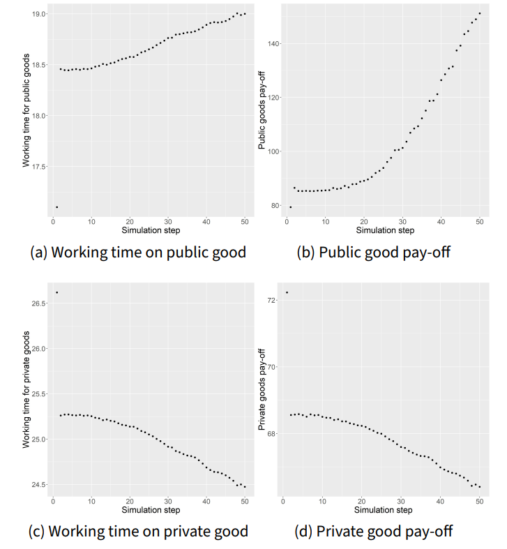
Discussion and Conclusions
The goal of this paper was to provide an analogy, in the sense defined by Edmonds et al. (2019), as to how different Schwartz values may influence the collective output measured across three dimensions: public goods provided, private goods provided and leisure time. We also show that population differences in the distributions of Schwartz values can lead to different behaviours of societies and eventually to differences in the collective output. It is considered important to look at the entire distributions of Schwartz values in the population, not only at the aggregates.
In this paper we proposed an agent-based model, in which the behaviour of the agents and the consequent interactions among them in two kinds of games (see below), depend on the Schwartz values. The major feature of the proposed model are as follows. We consider three types of occupation for the agents: worker, public goods manager and private goods manager. Agents may participate in both of the following games at the same time: a linear public goods game and a trust game. The agents decide how to divide their efforts between them. Local interactions are considered by taking the geographical distance, neighbourhood and travelling cost into account. The Roth-Erev reinforcement learning algorithm is implemented as an optimisation mechanism in the process of selecting the managers (working place) by workers. The data from the European Social Survey 9th round and the results from dedicated experiments were used to parametrise the model. We used the results of experiments we have conducted to derive and parametrise the respective behavioural rules.
The results provide a set of interesting insights about the relationships between personal values and work-related economic outcomes. The Schwartz values can be divided into two main groups, based on their effects on the collective output. The following variables belong to the first group: \(D_1\), \(D_2\) and \(D_4\). The first two variables measure the difference between two opposite higher order values: self-enhancement and self-transcendence. \(D_4\) measures the difference between the hedonism and conformity/tradition Schwartz values. The following variables belong to the second group: \(D_3\) and \(D_5\). Both variables measure the difference between two opposite higher order values: openness to change and conservation. The summary of the main results is provided in Table 16.
The most significant results are set out and compared to the existing literature in the following paragraphs. Firstly, we observe that an increased importance of achievement (and simultaneously a decreased importance of benevolence) leads to higher total working time. Furthermore, a greater importance of hedonism or stimulation (lower importance for tradition and conformity) generates the same effect. In this respect our findings are largely consistent with the literature. Emphasising achievement values, for example, is commonly associated with the business success of entrepreneurs who are likely to put relatively greater emphasis on work and are prone to experience a negative work-life balance (Chernyak-Hai & Tziner 2016; Gorgievski et al. 2011; Helmer & Olson 1987; Kasser et al. 2007). Moreover, business owners who are considered to have more active jobs (Stephan & Roesler 2010) can also reinforce the values of openness to change and de-emphasise the conservation values (Gorgievski et al. 2018), which can translate into an increased number of working hours in our study. Interestingly, among the conservative values the only one that drives people with a conservative orientation to spend more time working (in order to ensure financial stability for their families) seems to be that of security (Gerold & Nocker 2018). In the case of tradition (the other conservative value) our study supports evidence that this value is negatively related to working time – the tradition value itself shifts the available time towards family life rather than work, and can therefore prioritise a reduction in working hours (Gerold & Nocker 2018).
Secondly, some values may lead to opposite effects with respect to working time on public or private goods. In the case of public goods, our results reveal that an increased importance of self-enhancement and hedonism (decreased importance of self-transcendence) leads to higher working time, whereas a rise in the importance of openness to change (decrease for conservation) leads to lower working time. In general, previous studies demonstrate that contributing to public goods is usually associated with strong prosocial behaviours responding to the values of self-transcendence and conservation (Gorgievski et al. 2011; Sagiv et al. 2011). A typical example of such behaviour is that of perfect altruists who, by providing donations, are willing to increase the common pool while disregarding their private benefits (Gandullia et al. 2021). However, prosocial inclinations may also appear in people emphasising self-enhancement or openness to change values, such as imperfect altruists, who perform altruistic actions (e.g., make donations) to derive personal satisfaction or enhance their sense of belonging to the community (Gandullia et al. 2021).
In this context, our findings are compatible with the imperfect altruism by highlighting power, achievement, and hedonism as values that play a positive role in shaping contributions to public goods (when universalism, benevolence, conformity or tradition are simultaneously de-emphasised). Among conservative values, only increased security (simultaneously decreased self-direction) indicates an unambiguous and positive effect on the amount of time spent to provide public goods. Interestingly, precisely the opposite relationships between values and working time occur in the case of private goods. In this case, a greater emphasis on openness to change (with a corresponding decrease in conservation values) leads to longer working hours. As numerous studies reveal, individuals with self-direction or stimulation orientation are commonly characterised by creative performance, greater autonomy and a preference for unsystematic activities, rather than systematic or organised work (Arieli et al. 2020). Although this fact does not automatically determine the scale of the time division between work and leisure, it supports the intuition that people who avoid systematic and ambiguous work are likely to spend more time working, due to both the excitement and novelty from the actions taken and the search for innovative and challenging experiences, which requires a relatively large amount of work in itself.
From the pay-off perspective, the value patterns reveal a compatibility with those from total working time allocation to public or private goods respectively. This means that particular values have a reverse effect on the pay-off depending on what kind of goods (public or private) are considered. Interestingly, a pay-off generated by agents involved in public goods provision is higher when self-enhancement values are prioritised (self-transcendence values de-prioritised). This result could be linked to the general self-interest or profit-driven orientation of people pursuing power, achievement or hedonism (Gorgievski et al. 2011), regardless of the area in which they operate. In contrast, the opposite impact of self-enhancing values appears in the case of private goods. However, higher pay-offs from private goods are also associated with an emphasis on openness to change (stimulation, self-direction) and a simultaneously decreased importance of the conservation values (security, conformity and tradition). Pursuing stimulation and self-direction values satisfies an intrinsic need for the growth and autonomy of individuals, and relates positively to their subjective sense of well-being (Bobowik et al. 2011; Sortheix & Schwartz 2017). These relationships are also likely to translate into increased pay-offs in private goods provision.
Thirdly, the increase in pay-off inequality is positively associated with stimulation value orientations and negatively with those of achievement and hedonism, regardless of the type of goods (public or private) being provided. However, the type of goods play a role for other values and, due to the ambiguous role of tradition and conformity in shaping pay-off inequality, formulating our final conclusions in this respect requires due caution. Our simulation results find a partial confirmation (e.g., for power-universalism pair of values in private goods) in empirical evidence which indicates that societies with higher income inequality tend to be characterised by lower levels of self-transcendence and higher levels of conservative values (Tormos et al. 2017). In most cases, however, the results provide contrasting evidence. To some extent they may also be linked to some of the results by Schwartz & Bardi (2001) for societies with different GDP per capita levels. These results show that societies with high GDP per capita have higher levels of hedonism, stimulation, self-direction, benevolence and universalism, and lower levels of conformity, power, security and achievement (Schwartz 2004; Schwartz & Bardi 2001). Nevertheless, it should be noted that existing income inequalities are not only a result of a level of the economic development (GDP) but may also be caused by many other factors.
Finally, as we anticipated, the differences in value distribution within populations translate into differences in their economic performance. These findings indicate that an optimal mix of values may exist and serve to maximise the collective economic outputs or minimise inequalities in different social structures. In this respect, the results relate to a number of studies that emphasise the Schwartz values to be a driver of the economic development of societies and organisations, or the social well-being of individuals (Gorgievski et al. 2011; Sortheix & Schwartz 2017). The agent-based approach allows us to verify the value-economic performance relationship in a dynamic setting, and so derive a better understanding of the relationships observed in traditional experiments in this field.
The study presented contains a number of limitations, such as the limited number of public goods or private goods games, the fact that the experiments were restricted to student groups, or the simplified assumptions in the agent-based simulation. Nevertheless, the simulation results (which are mostly consistent with empirical observations and literature) confirm that agent-based modelling provides valuable complementary insights into the value-driven collective performance of societies, and thus holds implications for research, practice or policy, at both the macro and micro level.
Model Documentation
The code is written in Julia (Bezanson et al. 2017) and is available at: https://www.comses.net/codebases/7383e18b-33a8-465e-b0f6-346eef1f7c70/releases/1.0.0/.Acknowledgements
We thank Frederik Schaff and Michael Roos for discussions and all valuable comments. We also thank the attendees of the 2019 and 2022 Social Simulation Conferences for all the remarks and suggestions. We would also like to thank Timothy Harrell for his advice concerning matters of English usage.Funding>
This research was supported by a grant awarded by the National Science Centre of Poland under the project title "Values and Economic Performance: A formalised agent-based model" Decision no. 2018/31/G/HS4/01040.Notes
As Gandal et al. (2005) put it: “The relationships between the ten value types can be summarized into two basic conflicts. The first conflict is self-enhancement vs. self-transcendence. Self–enhancement values emphasize the pursuit of self-interest by focusing on gaining power and control over people and resources (power) or by demonstrating ambition and competence according to social standards and attaining success (achievement). These values conflict with self-transcendence values that emphasize serving the interests of others: expressing concern and care for those with whom one has frequent contact (benevolence) or expressing acceptance, tolerance, and concern for all people regardless of group membership (universalism). The second conflict is openness to change vs. conservatism: Openness to change emphasizes openness to new experiences: autonomy of thought and action (self-direction), novelty and excitement (stimulation). These values conflict with conservatism values that emphasize preserving the status quo: commitment to past beliefs and customs (tradition), adhering to social norms and expectations (conformity) and preference for stability and security for self and close others (security). Hedonism values share elements of both openness and self-enhancement and are in conflict with self-transcendence and conservatism values”.↩︎
To address the issue of multicollinearity one could use the three following methods: (i) remove some of the highly correlated variables; (ii) reduce the data dimensionality by the application of dedicated statistical methods, such as principal component analysis (or simply linearly combine the independent variables); (iii) apply the dedicated ridge regression estimator. (Greene 2003). The first method would require an arbitrary decision to remove some of the Schwartz values from the regression models and, consequently, accept that they bear no impact on the agents’ decisions. The second method may lead to the construction of new variables that would not be interpretable when principal component analysis is used. The third method may lead to biased estimators. Therefore, we followed the second approach – in a simplified version to preserve interpretability – and constructed the differences among Schwartz values which lie on opposite sides of the circle.↩︎
“When their [participants] value hierarchy was rendered accessible, participants explained their choices in terms of those values that were (a) important to them and (b) relevant to the situation. The findings thus point to the mechanism through which accessible values affect behavior” (Sagiv et al. 2011)↩︎
Importantly, “whether or not such games of trust are associated with trustworthy behaviour depends upon the players’ features and the game’s rules” (Witteloostuijn 2003).↩︎
Justification for the form of this function is provided in Section 3.10 in Equation 16, while the corresponding parameter values are presented in Table 2.↩︎
Expressions \(\textrm{max} \left(y_i^t -y_{-i}^t ,0\right)\) and \(\textrm{max} \left(y_{-i}^t -y_i^t ,0\right)\) are interpreted as \(z^+\) and \(z^-\) variables of the regression, with results presented in Table 2.↩︎
Analogously, as in the case of public goods, justification for the form of this function is subsequently provided and explained in Equation 17, while the corresponding parameter values are presented in Table 3.↩︎
Justification for the form of this function is provided later on, by the regression equation (Equation 18), while the parameter values are presented in Table 4.↩︎
References
ACEMOGLU, D. (2009). Introduction to Modern Economic Growth. Princeton, NJ: Princeton University Press.
AISEN, A., & Veiga, F. J. (2013). How does political instability affect economic growth? European Journal of Political Economy, 29, 151–167. [doi:10.1016/j.ejpoleco.2012.11.001]
ALESINA, A., & Giuliano, P. (2015). Culture and institutions. Journal of Economic Iiterature, 53(4), 898–944. [doi:10.1257/jel.53.4.898]
ALGAN, Y., & Cahuc, P. (2013). Trust and growth. Annual Review of Economics, 5(1), 521–549. [doi:10.1146/annurev-economics-081412-102108]
ARIELI, S., Sagiv, L., & Roccas, S. (2020). Values at work: The impact of personal values in organisations. Applied Psychology, 69(2), 230–275. [doi:10.1111/apps.12181]
ARIZA-MONTES, A., Arjona-Fuentes, J. M., Han, H., & Law, R. (2017). Employee responsibility and basic human values in the hospitality sector. International Journal of Hospitality Management, 62, 78–87. [doi:10.1016/j.ijhm.2016.12.001]
BARDI, A., Buchanan, K. E., Goodwin, R., Slabu, L., & Robinson, M. (2014). Value stability and change during self-chosen life transitions: Self-selection versus socialization effects. Journal of Personality and Social Psychology, 106(1), 131. [doi:10.1037/a0034818]
BARDI, A., & Goodwin, R. (2011). The dual route to value change: Individual processes and cultural moderators. Journal of Cross-Cultural Psychology, 42(2), 271–287. [doi:10.1177/0022022110396916]
BAUR, I., Dobricki, M., & Lips, M. (2016). The basic motivational drivers of northern and central European farmers. Journal of Rural Studies, 46, 93–101. [doi:10.1016/j.jrurstud.2016.06.001]
BECKER, G. S. (1965). A theory of the allocation of time. The Economic Journal, 75(299), 493–517.
BERG, J., Dickhaut, J., & McCabe, K. (1995). Trust, reciprocity, and social history. Games and Economic Behavior, 10(1), 122–142. [doi:10.1006/game.1995.1027]
BEZANSON, J., Edelman, A., Karpinski, S., & Shah, V. B. (2017). Julia: A fresh approach to numerical computing. SIAM Review, 59(1), 65–98. [doi:10.1137/141000671]
BOBOWIK, M., Basabe, N., Páez, D., Jiménez, A., & Bilbao, M. (2011). Personal values and well-being among Europeans, Spanish natives and immigrants to Spain: Does the culture matter? Journal of Happiness Studies, 12(3), 401–419. [doi:10.1007/s10902-010-9202-1]
BREWER, M. B. (2015). Individual values, social identity, and optimal distinctiveness. In C. Sedikides & M. B. Brewer (Eds.), Individual Self, Relational Self, Collective Self (pp. 233–252). London: Psychology Press.
BRÜLHART, M., & Usunier, J.-C. (2012). Does the trust game measure trust? Economics Letters, 115(1), 20–23.
CALLAGHAN, C. W. (2013). Individual values and economic performance of inner-city street traders. Journal of Economics, 4(2), 145–156. [doi:10.1080/09765239.2013.11884974]
CASTELLANI, M. (2019). Does culture matter for the economic performance of countries? An overview of the literature. Journal of Policy Modeling, 41(4), 700–717. [doi:10.1016/j.jpolmod.2018.06.006]
CHERNYAK-HAI, L., & Tziner, A. (2016). The “I believe” and the “I invest” of work-Family balance: The indirect influences of personal values and work engagement via perceived organizational climate and workplace burnout. Revista De Psicologdel Trabajo Y De Las Organizaciones, 32(1), 1–10. [doi:10.1016/j.rpto.2015.11.004]
CHIAPPORI, P.-A. (1988). Rational household labor supply. Econometrica, 56(1), 63–90. [doi:10.2307/1911842]
COHEN, A. (2009). A value based perspective on commitment in the workplace: An examination of Schwartz’s basic human values theory among bank employees in Israel. International Journal of Intercultural Relations, 33(4), 332–345. [doi:10.1016/j.ijintrel.2009.04.001]
CORNES, R., & Hartley, R. (2007). Aggregative public good games. Journal of Public Economic Theory, 9(2), 201–219. [doi:10.1111/j.1467-9779.2007.00304.x]
ČREŠNAR, R., & Nedelko, Z. (2020). Understanding future leaders: How are personal values of generations Y and Z tailored to leadership in industry 4.0? Sustainability, 12(11), 4417.
DAVIDOV, E., Schmidt, P., & Schwartz, S. H. (2008). Bringing values back in: The adequacy of the European Social Survey to measure values in 20 countries. Public Opinion Quarterly, 72(3), 420–445. [doi:10.1093/poq/nfn035]
DIRKS, K. T., & Ferrin, D. L. (2002). Trust in leadership: Meta-analytic findings and implications for research and practice. Journal of Applied Psychology, 87(4), 611. [doi:10.1037/0021-9010.87.4.611]
DUFFY, B. (2021). The Generation Myth: Why When You’Re Born Matters Less Than You Think. London: Hachette UK.
EDMONDS, B., Le Page, C., Bithell, M., Chattoe-Brown, E., Grimm, V., Meyer, R., Montañola-Sales, C., Ormerod, P., Root, H., & Squazzoni, F. (2019). Different modelling purposes. Journal of Artificial Societies and Social Simulation, 22(3), 6. [doi:10.18564/jasss.3993]
ELDER, G. H. (2018). Children of the Great Depression: Social Change in Life Experience. London: Routledge.
EPSTEIN, S., Pacini, R., Denes-Raj, V., & Heier, H. (1996). Individual differences in intuitive–experiential and analytical–rational thinking styles. Journal of Personality and Social Psychology, 71(2), 390. [doi:10.1037/0022-3514.71.2.390]
EREV, I., & Roth, A. E. (1998). Predicting how people play games: Reinforcement learning in experimental games with unique, mixed strategy equilibria. American Economic Review, 88, 848–881.
EVANS, J. S. B. (2008). Dual-processing accounts of reasoning, judgment, and social cognition. Annual Review of Psychology, 59, 255–278. [doi:10.1146/annurev.psych.59.103006.093629]
FARMER, J. D., & Foley, D. (2009). The economy needs agent-based modelling. Nature, 460(7256), 685–686. [doi:10.1038/460685a]
FLORES, N. E., & Graves, P. E. (2008). Optimal public goods provision: Implications of endogenizing the labor/leisure choice. Land Economics, 84(4), 701–707. [doi:10.3368/le.84.4.701]
GANDAL, N., Roccas, S., Sagiv, L., & Wrzesniewski, A. (2005). Personal value priorities of economists. Human Relations, 58(10), 1227–1252. [doi:10.1177/0018726705058911]
GANDULLIA, L., Lezzi, E., Parciasepe, P., & Siri, L. (2021). Altruism and structure of values: An experimental investigation. Journal of Interdisciplinary Economics, 33(1), 103–129. [doi:10.1177/0260107919897219]
GEROLD, S., & Nocker, M. (2018). More leisure or higher pay? A mixed-methods study on reducing working time in Austria. Ecological Economics, 143, 27–36. [doi:10.1016/j.ecolecon.2017.06.016]
GIGERENZER, G., & Gaissmaier, W. (2011). Heuristic decision making. Annual Review of Psychology, 62(1), 451–482. [doi:10.1146/annurev-psych-120709-145346]
GONZÁLEZ-RODRÍGUEZ, M. R., Diaz Fernandez, M. C., & Simonetti, B. (2016). Corporate social responsibility perception versus human values: A structural equation modeling approach. Journal of Applied Statistics, 43(13), 2396–2415.
GORGIEVSKI, M. J., Ascalon, M. E., & Stephan, U. (2011). Small business owners’ success criteria, a values approach to personal differences. Journal of Small Business Management, 49(2), 207–232. [doi:10.1111/j.1540-627x.2011.00322.x]
GORGIEVSKI, M. J., Stephan, U., Laguna, M., & Moriano, J. A. (2018). Predicting entrepreneurial career intentions: Values and the theory of planned behavior. Journal of Career Assessment, 26(3), 457–475. [doi:10.1177/1069072717714541]
GREENE, W. H. (2003). Econometric Analysis. London: Pearson Education.
GUISO, L., Sapienza, P., & Zingales, L. (2006). Does culture affect economic outcomes? Journal of Economic Perspectives, 20(2), 23–48. [doi:10.1257/jep.20.2.23]
HELMER, T., & Olson, S. F. (1987). The minority entrepreneur: An assessment of the correlation between personal values and company strategy. Southwest Academy of Management Sciences.
HITLIN, S. (2003). Values as the core of personal identity: Drawing links between two theories of self. Social Psychology Quarterly, 66(2), 118–137. [doi:10.2307/1519843]
HITLIN, S. (2008). Moral Selves, Evil Selves: The Social Psychology of Conscience. Berlin Heidelberg: Springer. [doi:10.1057/9780230614949_2]
INGLEHART, R. (2018). Culture Shift in Advanced Industrial Society. Princeton, NJ: Princeton University Press.
INGLEHART, R., & Abramson, P. R. (1994). Economic security and value change. American Political Science Review, 88(2), 336–354. [doi:10.2307/2944708]
INGLEHART, R. F. (2008). Changing values among western publics from 1970 to 2006. West European Politics, 31(1–2), 130–146. [doi:10.1080/01402380701834747]
JANSSEN, M. A., & Ahn, T.-K. (2006). Learning, signaling, and social preferences in public-good games. Ecology and Society, 11(2), 21. [doi:10.5751/es-01752-110221]
JANSSEN, M., & Baggio, J. A. (2016). Using agent-based models to compare behavioral theories on experimental data: Application for irrigation games. Journal of Environmental Psychology, 46, 106–115. [doi:10.1016/j.jenvp.2016.04.018]
JOHNSON, N. D., & Mislin, A. A. (2011). Trust games: A meta-analysis. Journal of Economic Psychology, 32(5), 865–889. [doi:10.1016/j.joep.2011.05.007]
KASSER, T., Cohn, S., Kanner, A. D., & Ryan, R. M. (2007). Some costs of American corporate capitalism: A psychological exploration of value and goal conflicts. Psychological Inquiry, 18(1), 1–22. [doi:10.1080/10478400701386579]
KELLEY, A. C., & Schmidt, R. M. (2005). Evolution of recent economic-demographic modeling: A synthesis. Journal of Population Economics, 18(2), 275–300. [doi:10.1007/s00148-005-0222-9]
KILEY, K., & Vaisey, S. (2020). Measuring stability and change in personal culture using panel data. American Sociological Review, 85(3), 477–506. [doi:10.1177/0003122420921538]
KNACK, S. (2001). Trust, assocational life, and economic performance.
KNACK, S., & Keefer, P. (1997). Does social capital have an economic payoff? A cross-country investigation. The Quarterly Journal of Economics, 112(4), 1251–1288. [doi:10.1162/003355300555475]
KONRAD, K. A., & Leininger, W. (2011). Self-enforcing norms and efficient non-cooperative collective action in the provision of public goods. Public Choice, 146(3), 501–520. [doi:10.1007/s11127-010-9600-2]
KRUGMAN, P. R. (1991). Increasing returns and economic geography. The Journal of Political Economy, 99(3), 483–499. [doi:10.1086/261763]
LANDES, D. S. (2015). Wealth and Poverty of Nations. London: Hachette UK.
LEDYARD, J. O. (1995). Is there a problem with public goods provision. The Handbook of Experimental Economics, 111–194.
LLOYD, P., & Lee, C. (2018). A review of the recent literature on the institutional economics analysis of the long-run performance of nations. Journal of Economic Surveys, 32(1), 1–22. [doi:10.1111/joes.12186]
MACAL, C. M. (2016). Everything you need to know about agent-based modelling and simulation. Journal of Simulation, 10(2), 144–156. [doi:10.1057/jos.2016.7]
MAGUN, V., & Rudnev, M. (2015). Basic human values of the russians.
MALE, S., & Stocks, R. (1989). Managers and the organisation. In P. M. Hillebrandt & J. Cannon (Eds.), The Management of Construction Firms (pp. 93–107). Berlin Heidelberg: Springer. [doi:10.1007/978-1-349-13626-1_7]
MAS-COLELL, A., Whinston, M. D., & Green, J. R. (1995). Microeconomic Theory. Oxford: Oxford University.
MASEL, J. (2007). A bayesian model of quasi-magical thinking can explain observed cooperation in the public good game. Journal of Economic Behavior & Organization, 64(2), 216–231. [doi:10.1016/j.jebo.2005.07.003]
MCCABE, K. A., Rigdon, M. L., & Smith, V. L. (2003). Positive reciprocity and intentions in trust games. Journal of Economic Behavior & Organization, 52(2), 267–275. [doi:10.1016/s0167-2681(03)00003-9]
MILES, L. D. (2015). Techniques of Value Analysis and Engineering. Mount Royal, NJ: Miles Value Foundation.
MINTZBERG, H. (1973). Nature of Managerial Work. New York, NY: Harper & Row.
NICHOLSON, W., & Snyder, C. M. (2012). Microeconomic Theory: Basic Principles and Extensions. Andover: Cengage Learning.
O’BRIEN, R. M. (2007). A caution regarding rules of thumb for variance inflation factors. Quality & Quantity, 41(5), 673–690. [doi:10.1007/s11135-006-9018-6]
ONES, U., & Putterman, L. (2007). The ecology of collective action: A public goods and sanctions experiment with controlled group formation. Journal of Economic Behavior & Organization, 62(4), 495–521. [doi:10.1016/j.jebo.2005.04.018]
PERRINJAQUET, A., Furrer, O., Usunier, J.-C., Cestre, G., & Valette-Florence, P. (2007). A test of the quasi-circumplex structure of human values. Journal of Research in Personality, 41(4), 820–840. [doi:10.1016/j.jrp.2006.10.006]
PIURKO, Y., Schwartz, S. H., & Davidov, E. (2011). Basic personal values and the meaning of left-right political orientations in 20 countries. Political Psychology, 32(4), 537–561. [doi:10.1111/j.1467-9221.2011.00828.x]
RODRIK, D., Subramanian, A., & Trebbi, F. (2004). Institutions rule: The primacy of institutions over geography and integration in economic development. Journal of Economic Growth, 9(2), 131–165. [doi:10.1023/b:joeg.0000031425.72248.85]
ROGERS, C. R. (1961). On Becoming a Person: A Therapist’S View of Psychotherapy. London: Constable.
ROOS, M. W. (2018). Endogenous economic growth, climate change and societal values: A conceptual model. Computational Economics, 52(3), 995–1028. [doi:10.1007/s10614-017-9707-3]
RUDNEV, M., Magun, V., & Schwartz, S. (2018). Relations among higher order values around the world. Journal of Cross-Cultural Psychology, 49(8), 1165–1182. [doi:10.1177/0022022118782644]
RUF, P. J., Graffius, M., Wolff, S., Moog, P., & Felden, B. (2021). Back to the roots: Applying the concept of individual human values to understand family firm behavior. Family Business Review, 34(1), 48–70. [doi:10.1177/0894486520944282]
SAGIV, L., Sverdlik, N., & Schwarz, N. (2011). To compete or to cooperate? Values’ impact on perception and action in social dilemma games. European Journal of Social Psychology, 41(1), 64–77. [doi:10.1002/ejsp.729]
SCHWARTZ, S. H. (1992). Universals in the content and structure of values: Theoretical advances and empirical tests in 20 countries. Advances in Experimental Social Psychology, 25, 1–65. [doi:10.1016/s0065-2601(08)60281-6]
SCHWARTZ, S. H. (1994). Are there universal aspects in the structure and contents of human values? Journal of Social Issues, 50(4), 19–45. [doi:10.1111/j.1540-4560.1994.tb01196.x]
SCHWARTZ, S. H. (1999). A theory of cultural values and some implications for work. Applied Psychology, 48(1), 23–47. [doi:10.1111/j.1464-0597.1999.tb00047.x]
SCHWARTZ, S. H. (2003). A proposal for measuring value orientations across nations.
SCHWARTZ, S. H. (2004). Mapping and interpreting cultural differences around the world. In H. Vinken, J. Soeters, & P. Ester (Eds.), Comparing Cultures (pp. 43–73). Leiden: Brill. [doi:10.1163/9789047412977_007]
SCHWARTZ, S. H. (2005). Robustness and fruitfulness of a theory of universals in individual values. Valores E Trabalho, 56–85.
SCHWARTZ, S. H. (2012). An overview of the Schwartz theory of basic values. Online Readings in Psychology and Culture, 2(1), 2307–0919. [doi:10.9707/2307-0919.1116]
SCHWARTZ, S. H., & Bardi, A. (2001). Value hierarchies across cultures: Taking a similarities perspective. Journal of Cross-Cultural Psychology, 32(3), 268–290. [doi:10.1177/0022022101032003002]
SCHWARTZ, S. H., Cieciuch, J., Vecchione, M., Davidov, E., Fischer, R., Beierlein, C., Ramos, A., Verkasalo, M., Lönnqvist, J.-E., Demirutku, K., Dirilen-Gumus, O., & Konty, M. (2012). Refining the theory of basic individual values. Journal of Personality and Social Psychology, 103(4), 663. [doi:10.1037/a0029393]
SORTHEIX, F. M., & Schwartz, S. H. (2017). Values that underlie and undermine well-being: Variability across countries. European Journal of Personality, 31(2), 187–201. [doi:10.1002/per.2096]
STEPHAN, U., & Roesler, U. (2010). Health of entrepreneurs versus employees in a national representative sample. Journal of Occupational and Organizational Psychology, 83(3), 717–738. [doi:10.1348/096317909x472067]
TORELLI, C. J., & Kaikati, A. M. (2009). Values as predictors of judgments and behaviors: The role of abstract and concrete mindsets. Journal of Personality and Social Psychology, 96(1), 231. [doi:10.1037/a0013836]
TORMOS, R., Vauclair, C.-M., & Dobewall, H. (2017). Does contextual change affect basic human values? A dynamic comparative multilevel analysis across 32 European countries. Journal of Cross-Cultural Psychology, 48(4), 490–510. [doi:10.1177/0022022117692675]
TORRES, C. V., Porto, J. B., Vargas, L. M., & Fischer, R. (2015). A meta-analysis of basic human values in Brazil: Observed differences within the country. Revista Psicologia Organizações E Trabalho, 15(1), 89–102. [doi:10.17652/rpot/2015.1.356]
VERPLANKEN, B., & Holland, R. W. (2002). Motivated decision making: Effects of activation and self-centrality of values on choices and behavior. Journal of Personality and Social Psychology, 82(3), 434. [doi:10.1037/0022-3514.82.3.434]
WEBER, J. (2017). Discovering the millennials’ personal values orientation: A comparison to two managerial populations. Journal of Business Ethics, 143(3), 517–529. [doi:10.1007/s10551-015-2803-1]
WECKROTH, M., & Kemppainen, T. (2016). Human capital, cultural values and economic performance in European regions. Regional Studies, Regional Science, 3(1), 239–257. [doi:10.1080/21681376.2016.1177467]
WITTELOOSTUIJN, A. van. (2003). A game-theoretic framework of trust. International Studies of Management & Organization, 33(3), 53–71. [doi:10.1080/00208825.2003.11043685]
WOJCISZKE, B. (1986). Teoria Schematów Społecznych: Struktura I Funkcjonowanie Jednostkowej Wiedzy O Otoczeniu Społecznym. Zakład Narodowy im. Ossolińskich.
YANDELL, B. S. (2017). Practical Data Analysis for Designed Experiments. Routledge.