An Exploration of Drivers of Opinion Dynamics

, , ,
and
aCopernicus Institute of Sustainable Development, Department Environmental Science, Utrecht University, Netherlands; bBiometris, Wageningen University & Research, Wageningen, Netherlands; cDepartment of Mathematics and Computer Science, Eindhoven University of Technology, Eindhoven, Netherlands; dDepartment of Industrial Engineering and Innovation Sciences, Eindhoven University of Technology, Eindhoven, Netherlands
Journal of Artificial
Societies and Social Simulation 27 (1) 5![]()
<https://www.jasss.org/27/1/5.html>
DOI: 10.18564/jasss.5212
Received: 16-May-2022 Accepted: 02-Aug-2023 Published: 31-Jan-2024
Abstract
Our ability to deal with external changes is determined by our collective willingness to transform and adopt new technologies. These factors are driven by people's opinion on the change itself and the proposed policies. Humans constantly update their opinion by integrating new information they hear with their values, which helps them make a judgement about that new information. Here, we create an agent-based model that explicitly incorporates the concept of values to explore possible drivers of opinion dynamics. In the model, we explore several factors and perform local and global sensitivity analysis to test their individual and interaction effects. We find that consensus formation in the model is mainly determined by factors related to (1) the amount of stochasticity in the opinion updating procedure and (2) the relative ease with which old links are removed and new links are created. Our results demonstrate how opinions and values may co-evolve. Furthermore, they may help in understanding human responses to new policies such as covid-related restrictions or calls to shift to a more plant-based diet.Introduction
Our ability to deal with external changes such as climate change, pandemics, and geopolitical developments, does not solely depend on the development of new technologies, but also on our collective ability to adopt new technologies (Alkemade & Coninck 2021). For decision makers this is an essential point: even if technologies potentially generate sufficient capability to deal with some external change, people have to adopt these technologies (Schlueter et al. 2012). This adoption is subject to various socioeconomic and social restrictions and trade-offs, including households’ economic limitations and personal values (FeldmanHall & Shenhav 2019; Schneider & Ingram 1990). An illustrative example is provided by the SARS-CoV-2 pandemic where the existence of a vaccine (technology) does not imply that people are also willing to take the vaccine (human behaviour) (Ebrahimi et al. 2021; Johnson et al. 2020). Another example, related to food choice, happened after publication of the EAT lancet report (Willett et al. 2019), describing the current state of scientific knowledge on healthy diets within environmental limits. In the weeks after publication, two twitter trends emerged: the hashtag #EATlancet welcomed the new insights, but was equally popular to the hashtag #yes2meat, which advocated for more meat consumption (Garcia et al. 2019). Webb et al. (2020) states that "Achieving transformation will require a major shift in mindsets" (Webb et al. 2020 p. 584). This raises the question why people respond differently to new technologies, and if and how a shift in the common mindset can be achieved that can then lead to mass adoption of new technology (so that people take the new vaccine, or adopt a new diet).
To explore the opinion forming process that might facilitate this social transformation, we first ask how individuals might adapt their opinion when interacting with others. According to Zaller (1991), people continuously adapt their opinions based on integrating new information they receive from the media and their peers, and their values that help them make a judgement about this new information. Using the definition of Zaller (1991), we see ‘values’ as “any relatively stable, individual-level predisposition to accept or reject particular types of arguments” (Zaller 1991 p. 1216). Thus, we consider interests, occupation, party membership and religion as examples of values that a person might have. Here, with the term values, we always mean the definition of Zaller (1991). In the English language, \(value\) can also refer to a numerical element (i.e. “the value for the parameter is 3”), but for clarity we will use the term \(number\) in those instances (i.e. “the number for the parameter is 3”).
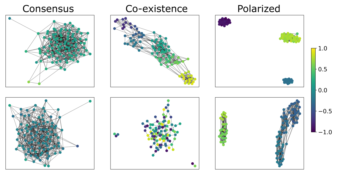
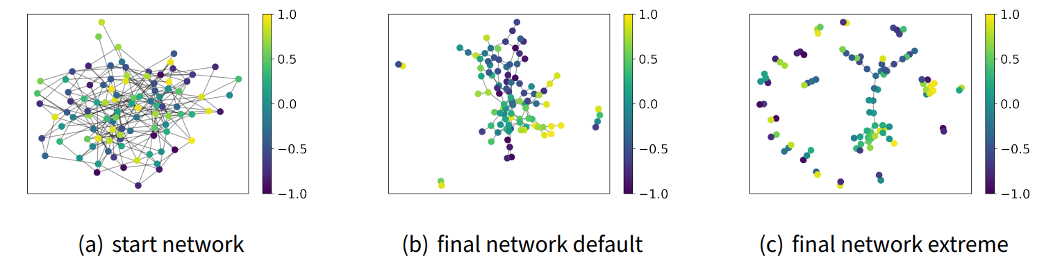
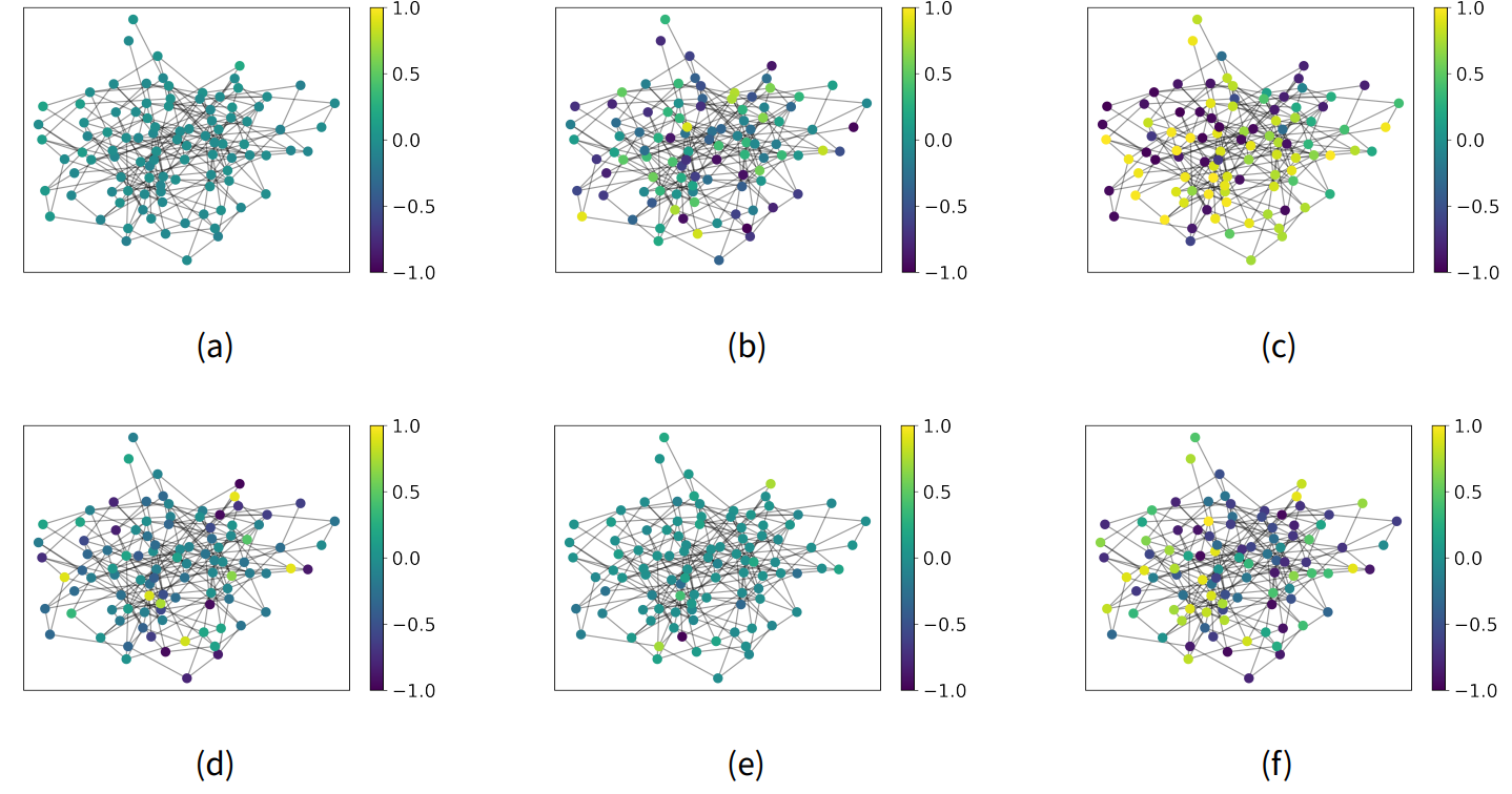
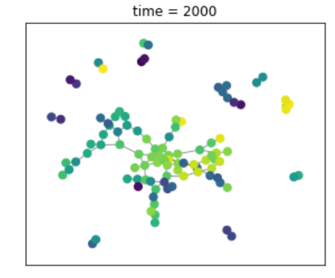
Models suggest that when it comes to dietary decisions, social norms in a group (closely related to the values of the group) have a larger effect on switching to more plant-based diets than factual information about health, sustainability and animal welfare (Eker et al. 2019). This is confirmed by empirical studies that show that people do indeed adapt their opinion and behaviour towards the people around them. For example, people that dine together adapt their food choice to match their dinner partner’s (Hermans et al. 2012; Pachucki et al. 2011). Therefore, explicitly incorporating values in opinion dynamics models and exploring how opinions and values may co-evolve seems like an important step forward in understanding opinion dynamics. Here, we study a simple opinion dynamics model that includes values and explore the drivers that may cause a community to reach one out of three qualitatively different states that were identified by Baron (2021): The Consensus state, the Co-existence state, and the Polarized state. In the consensus state, all agents have converged to one opinion. In the coexistence state, all opinions exist in the network and there is no clear clustering. Finally, in the polarized state, the network has clustered in two or more distinct groups (see Figure 1).
In this article, we will first provide the theoretical background that creates the basis for our model. Next, we describe our model based on the ODD protocol (Grimm et al. 2006) and describe the sensitivity tests that we use to analyze the model. Next, we provide the results of the model verification and local and global sensitivity analyses. Finally, we draw conclusions based on our results, discuss the implications of our findings and suggest future avenues for research.
Theoretical Background
The use of simple models for studying opinion dynamics has a long history (Flache et al. 2017) and has been inspired by models from statistical physics (Castellano et al. 2009). The simplest example is probably the Ising spin model, originally designed to describe the magnetization process in materials. In the Ising spin model, different ‘cells’ are connected to each other on a regular grid. Every cell has either an up or a down configuration (their spin). As time progresses, each cell tries to align its spin to its neighbors, leading to an ordered state with high magnetization (either all cells are up or all cells are down). When the temperature increases, cells start to flip up or down at random and the grid ends up in a disordered state (Wu et al. 1976). The same model has also been used as an illustration of opinion dynamics, where the cells represent individuals (or agents), and their spin is interpreted as an agent’s binary opinion (Castellano et al. 2009). The temperature parameter (\(T\)) then relates to the amount of stochasticity in the opinion dynamics: when \(T\) is low agents only update their opinion to align with their neighbors, and when \(T\) is high agents will change their opinion more randomly, for example, because of external stimuli that the model does not take into account, like reading the news, or mood swings.
For some decision making processes, these binary opinion models are useful approximations. This becomes especially fruitful when the opinion directly leads to a yes-or-no behaviour and the behaviour is the element of interest. For example, an individual may choose to get either vaccinated or not, but it is not possible to take half a vaccination. Other decision making processes however, require continuous opinion models (Flache et al. 2017). This relates for example to political left-wing right-wing choices (Deffuant et al. 2001), but also to decisions about food intake where people may choose to live anywhere on the ‘flexitarianism’ gradient (Kemper & White 2021), with a completely carnivorous or completely vegan lifestyle at the two extreme ends. Therefore, various modeling studies explore the effects of continuous opinions on the opinion dynamics. In the model of DeGroot (1974) for example, agents can take on any opinion on a continuous scale between -1 and 1. Next, their opinion dynamics are modeled by averaging between their own opinion and the opinion of their neighbors. If no node (or group of nodes) is disconnected from the network, consensus is reached as time progresses (DeGroot 1974). One extension to this model, called bounded confidence models, includes only the opinions of neighbors that are within a range \(r\) from one’s own opinion (Hegselmann & Krause 2002). For small values of \(r\), parts of the network become disconnected and no consensus is reached. Thus, ignoring opinions that are too dissimilar to one’s own opinion, allows for extreme opinions to persist (Deffuant et al. 2001; Hegselmann 2004). However, if new individuals with an opinion somewhere in the middle of the two opinions appear, they can ‘pull’ both extremes to the middle. Therefore, it seems that individuals with a nuanced opinion create cohesion, a result that is also found in simple models simulating decision making for gregarious animals, such as fish (Couzin et al. 2005).
One variation to the bounded confidence models are models where some individuals do not just ignore each other, but are repulsed by each other (Flache et al. 2017). Models that incorporate both repulsion (xenophobia) as well as attraction (homophily) are known as negative influence models (Flache et al. 2017). Conceptually, this repulsion can be a cause of cognitive dissonance (Festinger 1962) (i.e. “This person has such different values than I have, his/her opinion must be very different from mine”), or because of the need for people to belong to well-defined groups, that have clear rules about who does and who does not belong to that group (Brewer 1991). By emphasizing the differences to other groups, the within-group sense of identity may be preserved (Brewer 1991). A binary ABM that modeled within group attraction and between groups repulsion resulted in polarized states that have maximized their difference in opinion (Macy et al. 2003). A model where agents could also take an ‘undecided’ opinion allowed for consensus to exist (Balenzuela et al. 2015), just like in continuous bounded confidence models. In continuous models that include repulsion based on dissimilarity between individuals, both consensus states as well as polarized states into two or more groups can be observed (Jager & Amblard 2005; Salzarulo 2006).
Lastly, our model is inspired by a type of model where the repulsion is modeled dynamically and individually for all agents, as for example done by Huet & Deffuant (2010). In their work, Huet & Deffuant (2010) noted that people may be attracted to an unlikely opinion, if that opinion comes from a group with whom they share values. They built a model in which all agents had two continuous opinions, one on a main and one on a secondary axis. If two agents’s opinions were similar on the main axis, then they would align their opinions on both axes. However, if their opinions differed on the main axis, they would diverge their opinion on the secondary axis and ignore each other on the main axis. In this way, polarization in secondary opinion would occur if agents differed in their opinions on their main axes (depending on the threshold parameters).
Using the above mentioned models as inspiration, we created an ABM that helped us explore the effects of the proposed drivers of opinion dynamics. We extend on these models to incorporate the concept of values and continuous opinions to study opinion dynamics. Particularly, we explore the relationships between and the effects of three different types of variables: firstly the opinions (a fast changing element), secondly the values (a slow changing element), and thirdly variability in personality traits (a static element). The values in our model can be seen as the main opinion axis in the Huet & Deffuant (2010) model. For all agents, their values are slowly aligning with the values of their neighbors (like in the DeGroot (1974) model). This differs from the Huet & Deffuant (2010) model because we never ignore neighbors. However, we work on a dynamical network, so it is possible for agents to cut-off links to other agents (effectively ignoring them). In time, values converge to one another for the parts of the network that are connected. Our opinion dynamics process works on top of that. Agents adapt their opinion towards neighbors with similar values (attraction), but they will adapt their opinion away from neighbors with a different value (repulsion). This step has a stochastic component: depending on the temperature of the system, agents may change their opinion at random. This stochasticity provides an additional distinction between the slowly changing values that change in a deterministic way and the fast changing opinions that may change in a stochastic way (i.e. opinions are more volatile than values). The distance in values where agents still align with their neighbors is similar to the \(r\) in bounded confidence models from Hegselmann & Krause (2002) (indicating the maximum opinion distance that still leads to attraction, see section 2.2), with two main differences: 1) In our model, \(r\) looks at the values of the neighbors instead of the opinions, and 2) for neighbors whose value differs more than \(r\), our agents actively move away, whereas in the bounded confidence models they just ignore this neighbor. Since this process is related to cognitive dissonance (see Section 2.3), instead of \(r\), we call this parameter ‘\(dist\_cd\)’, indicating the distance of cognitive dissonance. By incorporating some static personality traits, we are able to tune how heterogeneous our population is. The traits that we implement are stubbornness (how likely it is that an agent will change his/her opinion) and persuasiveness (how much influence an agent has to change the opinion of others). When compared to the model from Huet & Deffuant (2010), our model has two main differences: 1) we simulate a dynamical network, meaning that links can be created and removed in time, and 2) our opinion updating procedure is stochastic so we can explore the influence of noise on the system. An extensive description including an ODD protocol is provided in the methods section of this paper.
We will use this model to determine which factors are the main drivers that push the system into either the consensus, co-existence, or polarized state (see Figure 1) and to identify sources of uncertainty in opinion dynamics.
Methods
Model description
In this section, we describe our model using the ‘ODD’ (Overview, Design concepts & Details) protocol as proposed in 2006 by Grimm et al. (2006) and updated in 2010 (Grimm et al. 2010).
- Purpose The purpose of our model is ‘theoretical exploration’, i.e. to explore the relations between some isolated and combined mechanisms and their implications in the opinion forming process (Edmonds et al. 2019). The mechanisms of interest are the creation of new links (forming of new interactions), the removal of old links (losing interactions), the slow change of values, and the effects of social influence on opinion dynamics.
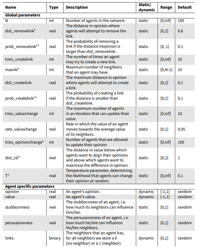
- Entities, state variables & scales The main entities in our model are human agents. Every agent has a number for their current opinion, their current value, and a static number for two personality traits, namely stubbornness and the persuasiveness. Another important variable is the ‘temperature’ of the system. This is a global parameter representing to what extent agents adapt their opinion to others. In line with the Ising spin model, a high temperature indicates less matching to the neighbors and more random fluctuations. We implement time in discrete steps. The time scale is arbitrary, as the importance is the relative rates in which the opinions and values change and not their absolute rate. However, one full simulation (2000 time steps) can be considered to model dynamics of processes in the order of magnitude of years. A full list of input parameter is provided in Table 1. Default numbers are chosen in such a way that at default settings, the three states (consensus, co-existence, and polarized, see Figure 1) can all be observed.
- Process overview and scheduling The model starts with an initial network with a set configuration (see step 5: initialization). Then at each step in time, four submodules are executed. First, all agents may remove links with neighbors whose opinions are dissimilar (distance larger than \(dist\_removelink\)). Secondly, all agents may create new links with agents who are similar to them (distance smaller than \(dist\_createlink\)). Thirdly, a certain number of randomly picked agents may update their value to match the value of their neighbors. Lastly, a certain number of randomly picked agents may update their opinion based on their stubbornness (the more stubborn, the less likely they will change their opinion), their neighbors values and opinions, and their neighbors persuasiveness (the higher the persuasiveness, the more effect a neighbor has on an agent).
These modules are described in more detail in step 7 of the ODD protocol. - Design Concepts
- Basic Principles In line with the model of DeGroot (1974), we assume opinions can be represented on a continuous scale from -1 to 1. Opinions of -1 and 1 represent the extreme opinions, whereas an opinion of 0 represents no preference for either side. Our network consists of bidirectional links only, therefore if agent A is linked to agent B, agent B is linked to agent A as well. We do not allow agents to lose all connections and we set the maximum number of neighbors to \(maxnb\), so all agents have between 1 and \(maxnb\) neighbors. The parameter \(maxnb\) is our model equivalent of ‘Dunbars number’, which is the maximum number of close interactions a person can have (this is found to be 150 in the real world) (Dunbar 2010).
- Emergence The distributions of values and opinions over time, as well as the network configurations are emergent properties of the model.
- Adaptation Agents remove and create new links in the network. Furthermore, they slowly change their values to match their neighbor’s values. Last, they minimize their opinion distance to neighbors with a similar value while maximizing their opinion distance to neighbors with a different value.
- Objectives We model social influence by letting agents adapt their opinions towards neighbors with a similar value and away from neighbors with a different value. Agents enter this opinion updating procedure with a probability of 1-\(stubbornness\) (i.e. stubborn agents never update their opinion, unstubborn agents often update their opinion). Then, we allow agents to change their opinion, which happens based on the values and opinions of their neighbors. All agents try to maximize their opinion distance to neighbors with value distance (\(|value_i - value_j|\)) larger than \(dist\_cd\), and minimize their opinion distance to neighbors with value distance smaller than \(dist\_cd\). Thus, when agents are confronted with arguments that do not match their way of reasoning, i.e. their value, they actually move away from the opinion they are hearing (Festinger 1962). We perform this minmizing/maximizing step by calculating the “imbalance” of the network (in Ising spin terminology this is commonly referred to as the energy of the system). To calculate the imbalance, we first need to know whether to minimize or to maximize the distance, so we calculate
where \(valuesigns_{ij}\) is the valuesign between agents \(i\) and \(j\) and \(\theta(x)\) is the heaviside function which is 0 if \(x<0\) and 1 if \(x>0\) . \(valuesigns_{ij}\) is 0 if the values of agent \(i\) and agent \(j\) have a distance that is smaller than \(dist\_cd\) and 2 if their values have a distance that is larger than \(dist\_cd\). Next, the total imbalance can be calculated as\[valuesigns_{ij} = -2 * \theta(dist\_cd - |value_i - value_j|)+2,\] \[(1)\]
where \(|opinions_i - opinions_j|\) is the distance of opinions between agents \(i\) and \(j\). If the values of the two agents vary more than \(dist\_cd\), \(valuesigns_{ij}\) is 2. In this case \(|valuesigns_{ij} - |opinions_i - opinions_j||\) is 0 when \(opinions_i\) and \(opinions_j\) are furthest away from each other (-1 and 1). When the two values are within a range of \(dist\_cd\), \(valuesigns_{ij}\) is zero. In this case, \(|valuesigns_{ij} - |opinions_i - opinions_j||\) is 0 when \(opinions_i = opinions_j\). Finally, the effect is multiplied by the persuasiveness of agent \(j\). Thus, agents with a high persuasiveness have a larger influence on the opinion change than agents with a low persuasiveness.\[I = \sum_{i=1}^{N} \sum_{j=1}^{i} |valuesigns_{ij} - |opinions_i - opinions_j|| * persuasiveness_j, \] \[(2)\]
Based on these calculations, when there is full consensus among neighbors, the imbalance is low, while when there is disagreement between neighbors, the imbalance is high. - Learning Not applicable.
- Prediction Not applicable.
- Sensing Agents change their opinions based on their own opinions, values, and stubbornness, and the opinions, values, and persuasiveness of their neighbors. Thus they ‘sense’ this information about themselves and about their neighbors. Furthermore, they may create links to non-neighbors based on the opinions of these non-neighbors. Thus, they sense the opinions of all other agents.
- Interaction Agents interact with their neighbors through bidirectional links. These links can be removed or created in submodules 1 and 2 respectively. In these interactions they will align their values and they might converge or diverge their opinions.
- Stochasticity Stochasticity comes from multiple sources. Creating and removing links happens with an initialized probability, entering the opinion-changing module happens with a probability that depends on an agent’s stubbornness. Also, in line with the Ising model, agents may change their opinion with a probability that depends on the ‘temperature’ (the higher the temperature, the less they take their neighbors’ opinions into account). Last, in submodules 3 and 4 a predefined number of agents is chosen at random to update their values and opinions.
- Collectives Not applicable.
- Observations The data that we collect from our model are 1) the opinions of all agents over time, 2) the values of all agents over time, and 3) the network over time. For computational efficiency, we do not save all information, but instead we extract this information at the start and at the end of the simulation. The simulation ends when it does not change for 200 iterations or after 2000 iterations. We say the simulation is unchanged when the Wasserstein distance (also known as Earth Mover’s distance) between consecutive distributions of opinions from the 100 agents is smaller than 0.003.
From the opinions of the agents, we calculate in which state the networks belongs: If the opinion distribution has 1 peak and a low variance it belongs in the consensus state, of the opinion distribution has 1 peak and a high variance it belongs in the co-existence state, and when the opinion distribution has more than 2 peaks it belongs in the polarized state. This categorization of the opinion distributions is further clarified and visualized in appendix A.
- Initialization Before a simulation is run, all parameters need to be initialized. Default numbers are depicted in table 1. Furthermore, every agent is given a number for stubbornness, persuasiveness, opinion, and value sampled from uniform distributions. Last, an initial network of links is created at random, where the probability of forming a link between any two agents is set at 0.05 (leading to an average degree of 5 links per agent when \(N=100\)).
- Input data Not applicable.
- Submodules The four submodules as presented in step 3 are called consecutively and have been implemented as follows:
- Remove links For every agent, check the distance from the agent’s opinion towards the opinion of all neighbors. If the distance in opinion is larger than \(dist\_removelink\), remove the link with a probability of \(prob\_removelink\).
- Create links For every agent with less than \(maxnb\) neighbors, pick another agent at random. If the new agent has an opinion within a distance \(dist\_createlink\), create a new link with a probability of \(prob\_createlink\). Repeat this procedure \(tries\_createlink\) times per agent.
- Update values For \(tries\_valuechange\) agents, calculate their optimal value by averaging the value of their neighbors. Take a step of \(rate\_valuechange\) towards the optimal value.
- Update opinions For \(tries\_opinionchange\) agents, with a probability of \(1-stubbornness\), create a temporary new opinion \(new\_op\), drawn from a uniform distribution on [-1,1]. Then calculate the total imbalance with the current opinion (\(I\_old\)) and with the new opinion (\(I\_new\)) with equation 2. Calculate \(\Delta I\) as \(I\_new - I\_old\). If \(\Delta I < 0\), change the opinion of the agent to \(new\_op\). If \(\Delta I > 0\), change the opinion of the agent to \(new\_op\) with a probability of \(e^{-\Delta I / T}\). We should point out three features. Firstly, the new opinion is generated at random, so it does not necessarily lie in between the opinions of the neighbors of the focal agent. The idea behind it is that people hear opionions everywhere around them (i.e. tv, newspapers, commercials). In our model, this is represented by the stochastic nature of the random choice of \(new\_op\). Whether the agents stick to this new opinion is based on how it fits within the network. Thus, \(new\_op\) is not created based on neighbors, but the neighbors help decide whether or not the \(new\_op\) stays. It is a way of adding variability to the model without having to implement additional details (such as tv or newspapers). Secondly, the role of the temperature parameter \(T\) is to determine the level of stochasticity. When \(T=0\), only opinions that lower the imbalance are accepted. As \(T\) increases, opinions that increase the imbalance have an increasing probability of acceptance as well. Thirdly, for \(T\neq0\), the probability of accepting a \(new\_op\) that increases the imbalance, depends on how much it increases the imbalance. Therefore, when two agents already agree to a large extend, the probability of changing their opinion becomes smaller.
The model is implemented in Python 3.8 by one of the authors and reviewed by another author to verify both correctness and clarity. The code used for the analysis and a jupyter notebook with examples can be downloaded from: https://github.com/elsweinans/opinion_dynamics. For the figures in Appendix B a seed is set so they are exactly replicable. The other simulations might differ slightly due to the random numbers used, but can all be reproduced qualitatively with the provided code.
Model exploration
We test the model in three ways.
Firstly, we run all submodules in isolation of the other submodules to verify if the produced behaviour by each submodule is as expected.
Secondly, we perform global sensitivity analysis to understand which input parameters influence the opinion dynamics the most. We apply PAWN (Pianosi & Wagener 2018) as implemented in the SALib library (Herman & Usher 2017) to estimate the total importance of each input parameter. The data is generated using Latin Hypercube Sampling (McKay 1992) through the Exploratory Modelling & Analysis Workbench (Kwakkel 2017). The sensitivities are calculated over 10 000 samples (input parameter combinations), each with 10 replications under random initial conditions. The probability of a certain network state across these 10 replications for each sample is used as the dependent variable in the analysis. The resulting sensitivities are validated by verifying their convergence (Sarrazin et al. 2016).
Thirdly, we perform one-factor at a time (OFAT) sensitivity analysis as recommended by ten Broeke et al. (2016) (among others) to explore the effect of seven parameters in the model (\(tries\_opinionchange\), \(dist\_cd\),
\(dist\_removelink\), \(T\), \(maxnb\) and the combined set of \(prob\_removelink\) and \(prob\_createlink\), marked with a * in Table 1) on the probability of ending up in each of the three states of Figure 1. These parameters were chosen based on the global sensitivity analysis, which indicated them as dominant drivers that determined the final state of our simulations.
Results
Verification of individual submodules
We test the different submodules separately to (1) assess whether they behave as they should, and (2) determine, at a later stage, which submodule is responsible for which behaviour once all modules are included in the model. Our results demonstrate that all modules behave as expected (see Appendix B for visualizations of all verification steps and additional explanation).
Global sensitivity analysis
Our PAWN global sensitivity analysis reveals that \(T\) is the most important parameter in our model, strongly influencing the likelihood of occurrence of all three states. This parameter is especially powerful in distinguishing the co-existence state from the consensus and polarized states (Table 2). Other parameters that are influential are \(tries\_opinionchange\), \(dist\_cd\), \(dist\_removelink\), \(maxnb\) and \(prob\_changelink\) (which determines both \(prop\_createlink\) and \(prob\_removelink\)) (Table 2). These are also the parameters that we explore in more detail in the OFAT sensitivity test in the next subsection.
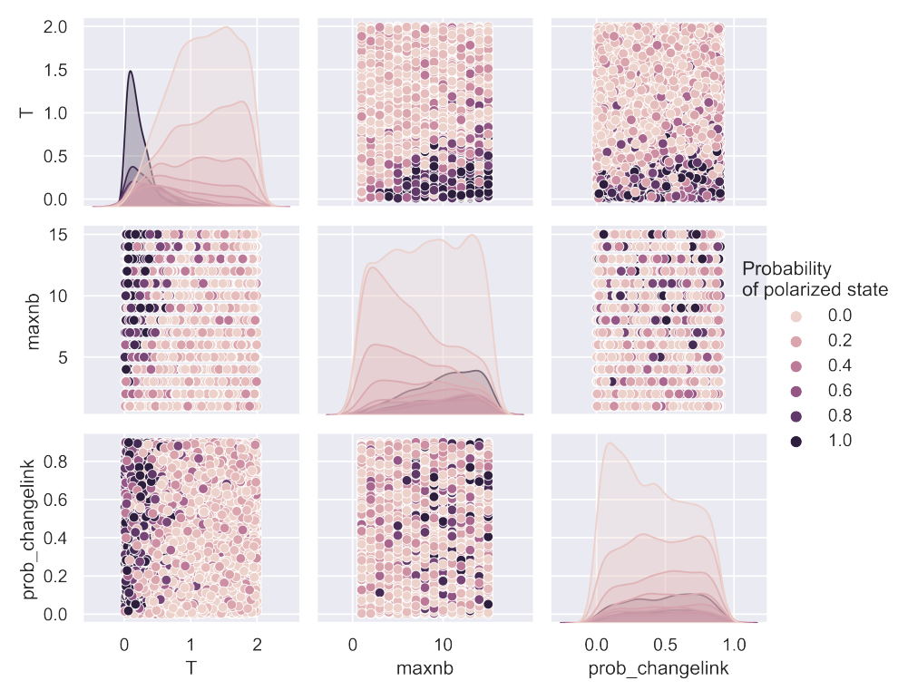
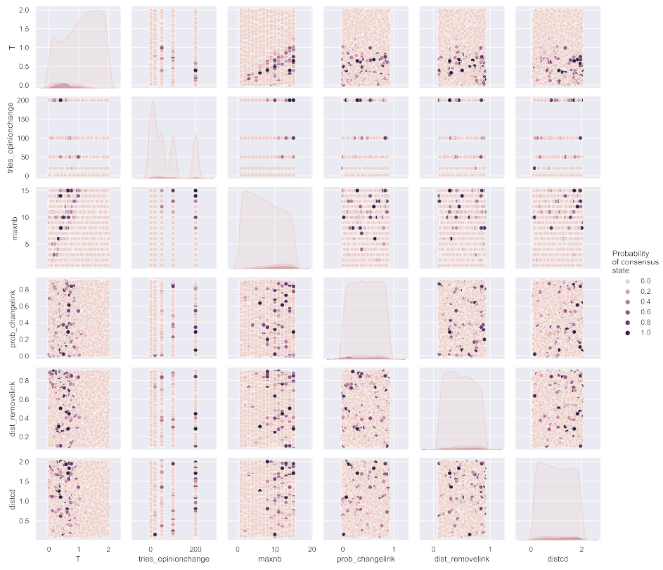
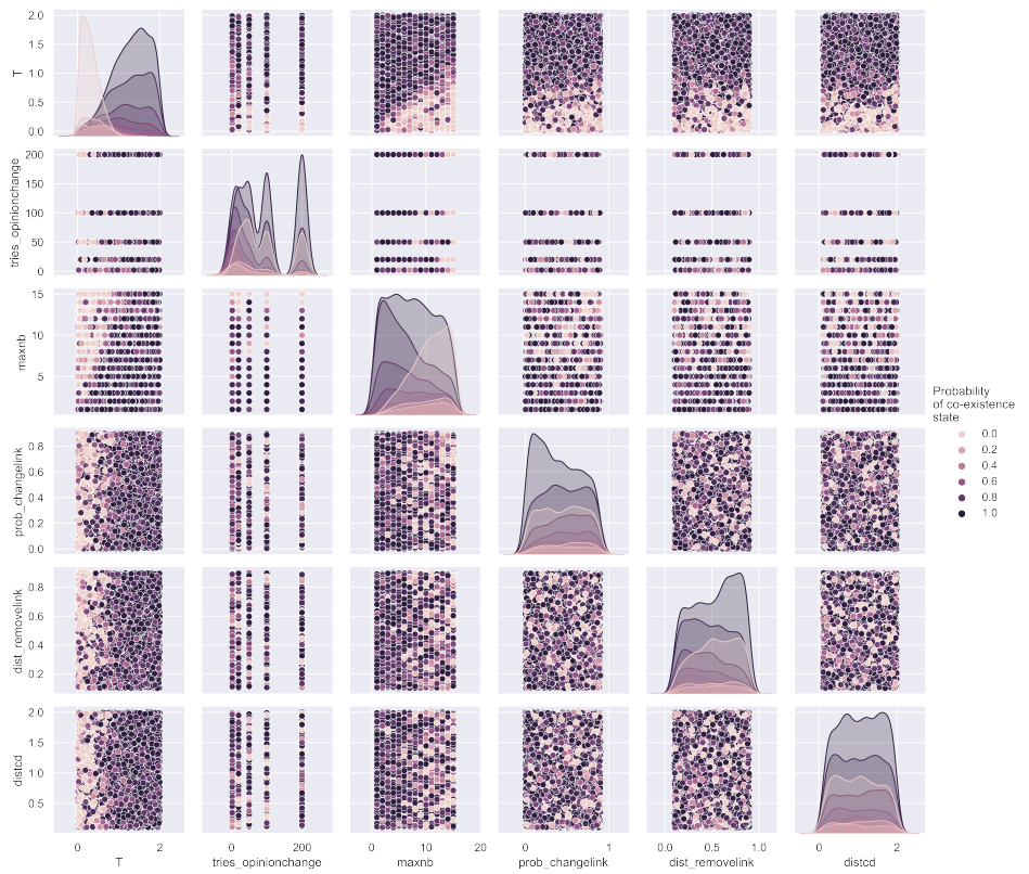
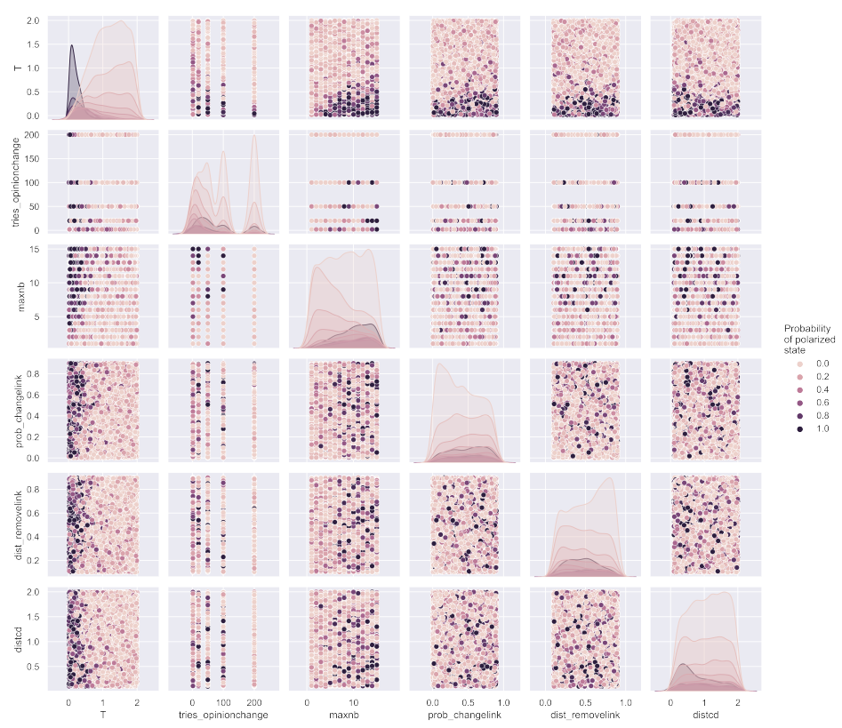
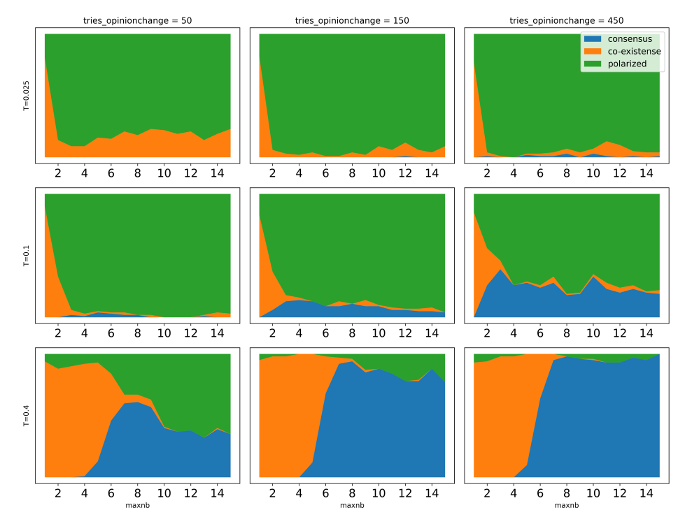
The PAWN sensitivities describe total sensitivities. To explore whether the parameters work in isolation or if there are second order interaction effects, we create pairplots based on the 10 000 samples. For every sample with 10 replicates, we calculate the probability of ending up in each of the three states. Most parameters do not seem to have strong second order interaction effects (supplementary Figures 9- 11) with the exception of the parameters \(T\) and \(maxnb\). We find that for low numbers of \(T\), the polarized state is the most likely state (Figure 11). As \(T\) increases, the consensus state becomes dominant (Figure 9). For even higher numbers of \(T\), the co-existence state becomes dominant (Figure 10). The boundary for these switches lies at higher numbers of \(T\) for increasing numbers of \(maxnb\) (and, less pronounced though, for decreasing numbers of \(tries\_opinionchange\)). The parameter \(prob\_changelink\) seems important based on its occurrence (diagonal plot for \(prob\_changelink\) in supplementary Figures 10- 11), but does not seem to have second order interactions with the other parameters. For \(T\), \(maxnb\), and \(prob\_changelink\), we summarize this information for the polarized state in Figure 2.
Higher order effects could be present as well, but cannot be revealed with the presented analysis. In our OFAT analysis we explore this option further.
| State | |||
|---|---|---|---|
| Parameter | Consensus | Co-existence | Polarized |
| T | 0.15 | 0.28 | 0.19 |
| tries_opinionchange | 0.06 | 0.08 | 0.11 |
| maxnb | 0.09 | 0.13 | 0.09 |
| prob_changelink | 0.01 | 0.05 | 0.06 |
| dist_removelink | 0.05 | 0.04 | 0.05 |
| dist_cd | 0.04 | 0.02 | 0.04 |
| dist_createlink | 0.02 | 0.03 | 0.04 |
| tries_createlink | 0.01 | 0.03 | 0.04 |
| rate_valuechange | 0.01 | 0.03 | 0.03 |
| tries_valuechange | 0.01 | 0.02 | 0.02 |
OFAT sensitivity tests
To explore the extent to which the parameters \(tries\_opinionchange\), \(dist\_cd\), \(dist\_removelink\), \(T\), \(maxnb\) and the combination of \(prop\_createlink\) and \(prob\_removelink\) affect the final configuration of the network on which opinions and values co-evolve, we slowly change these parameters in a stepwise fashion and run 100 simulation for every parameter number. Then, we calculate the probability of the system to end up in each state of Figure 1.
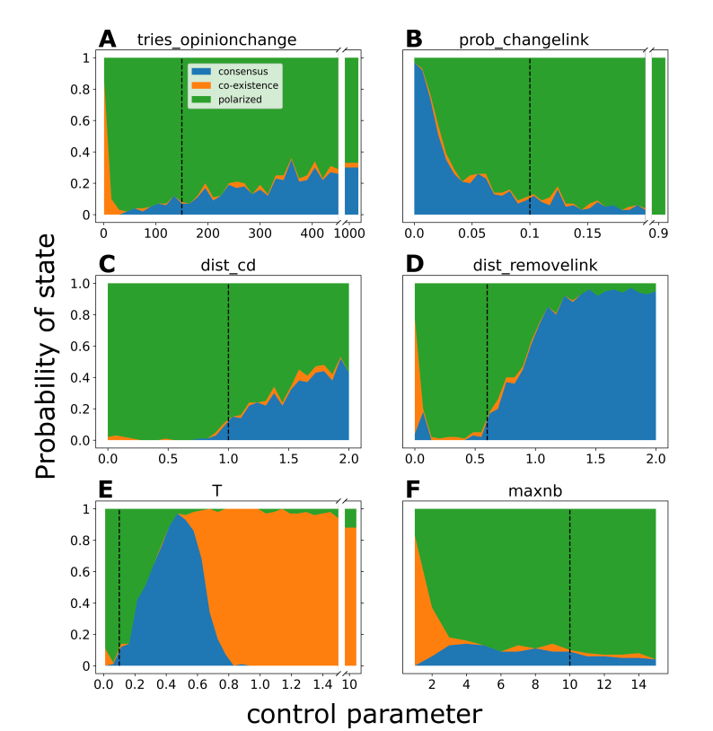
We find that at the low extreme end of \(tries\_opinionchange\), the network has the highest probability of ending up in the co-existence state. As \(tries\_opinionchange\) increases, the polarized state takes over. Then, from \(tries\_opinionchange = 50\) onwards, we observe a steady increase of the consensus state. However, for all numbers where \(tries\_opinionchange > 1\), the largest percentage of simulation is made up by the polarized state. This means that for the default parameter settings, the network is most likely to end up in the polarized state and although \(tries\_opinionchange\) does affect the relative probabilities, the polarized state remains the most likely final state of the network (Figure 3A).
For low numbers of \(prop\_createlink\) and \(prob\_removelink\) (referred to as \(prob\_changelink\)) the system is most likely to end in the consensus state. As \(prop\_changelink\) increases, the consensus state becomes less likely to occur. For numbers of \(prob\_changelink\) higher than 0.025, most simulations end up in the polarized state, with a small fraction for the other two states throughout the tested range (Figure 3B). The probability of removing or adding a link affects the final network configurations through the values. Because the values between neighbors change very slowly, they only converge when two agents stay connected for a long time (i.e. when \(prop\_changelink\) is low).
For low numbers of \(dist\_cd\), the system is most likely to end up in the polarized state. For numbers of \(dist\_cd\) higher than 0.8, we observe a rise of the occurrence of the consensus state (Figure 3C). For the maximum number of \(dist\_cd\), 2 (i.e. when values and cognitive dissonance do not play a role anymore), we find that our simulations are equally likely to end up in the consensus- and the polarized state (Figure 3C).
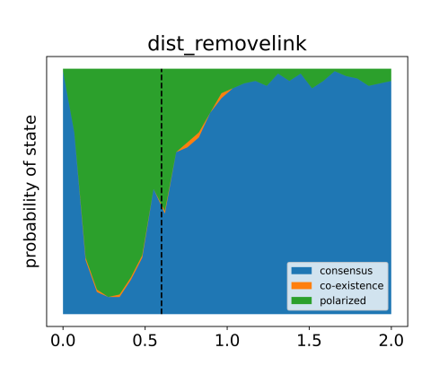
At the low extreme end of \(dist\_removelink\), our model is most likely to end up in the co-existence state. Very quickly however, the polarized state becomes dominant. At the lower end there is a small probability of the consensus state, but for numbers of \(dist\_removelink\) higher than 0.1 this state disappears. It reappears around \(dist\_removelink = 0.5\), and after that, the consensus state becomes the most likely outcome of the simulations (Figure 3 D). To get a better understanding of the low end of this graph, we visualize a final network where \(dist\_removelink = 0\) (supplementary Figure 13). We observe that in this situation, there are many agents with only one neighbor. Furthermore, we repeat the \(dist\_removelink\) OFAT, but now for \(dist\_createlink = 0.6\) (instead of the default of 0.3). Here, we observe that the probability of consensus is higher, this effect is particularly strong for the left half of the OFAT plot (supplementary Figure 14).
For low numbers of \(T\), the system is most likely to end up in the polarized state. As \(T\) increases, the consensus state appears. The probability of ending up in the consensus state peaks at \(T=0.5\). After this, the likelihood of consensus decreases and the co-existence state becomes the most likely final state of the system (Figure 3E). This confirms our observation from the global sensitivity test.
For low numbers of \(maxnb\), our model is most likely to end up in the co-existence state. As \(maxnb\) increases, the consensus and polarized states become more likely. The rise in polarization is more pronounced and for the largest range of \(maxnb\), the polarized state is the most likely final state of our model (Figure 3F). Our pairwise plots from the global sensitivity tests suggest that the number of \(maxnb\) where co-existence disappears will be higher when the parameter \(T\) increases.
We note that the OFAT analysis works as a sanity check for our PAWN sensitivity test: The OFAT plots can be seen as transects along the default numbers in the two-parameter PAWN figures (Figure 2 and Figures 9- 11). This is not a one-to-one relationship, because in the PAWN test the other parameters are chosen freely, thus exploring the whole range of possible numbers, whereas in the OFAT plots the other parameters are fixed at their default. Still, certain properties of our model are clearly visible in both PAWN and OFAT sensitivity tests, demonstrating robust results. One clear illustration is the \(maxnb\) plot, where Figure 2 illustrates how at \(T=0.1\) (default) the probability of the polarized state is low for \(maxnb<3\) and becomes high for \(maxnb>3\). This result is replicated by the OFAT test for maxnb (Figure 3F). The comparison between PAWN and OFAT thus gives additional insight in the non-linear effects that the parameters have on the model output.
Lastly, we test for three way interactions between the three most important parameters (\(T\), \(tries\_opinionchange\), and \(maxnb\)) by repeating the OFAT analysis of \(maxnb\) for different combinations of \(T\) and \(tries\_opinionchange\). We observe that the highest probability of the consensus state is reached when all three parameters are at high numbers, representing a three way interaction between the three variables (see: Appendix D).
Discussion
Summary of results
In this paper we considered the co-evolution of values and opinions on a dynamical network. We constructed an ABM derived on models from statistical physics, and expanded it to continuous opinions and included a fast-changing (opinions), slow-changing (values), and static variable (personality traits) and a dynamical social network. Because the slow change of the values, they can only create convergence of opinions, when two agents stay connected for a long time. As such, values strengthen the status quo of the network. In combination with the dynamic nature of our network, various outcomes may arise. Our results suggest that consensus of opinions can happen, but that the full spectrum of opinions or even two or more distinct, stable opinions are possible outcomes as well. Sensitivity analyses (based on PAWN & OFAT) were used to identify the main drivers of opinion dynamics in our model. We found that in order to reach the consensus state, agents should 1) update their opinion often (Figure 3A), 2) do not often break links and create links to new agents (figure 3B), 3) adapt their opinion to their neighbors regardless of their values (i.e. high \(dist\_cd\), Figure 3C), 4) only remove links to people that are very dissimilar to them (Figure 3D), and 5) preferably have some sources of information that affect their opinions that our model does not take into account (i.e., intermediate stochasticity/\(T\), Figure 3E).
Both the global sensitivity (PAWN) test and the OFAT test revealed that the parameter \(T\) is an important driver of opinion dynamics. This parameter determines the level of stochasticity in the model, i.e. for high numbers of \(T\), agents will update their opinion at random, independent of the values of their neighbors, and for low numbers of \(T\), agents only update their opinion to better (dis)align with their neighbors, driven by the difference in values between the agent and its neighbors. Counter intuitively, intermediate numbers of \(T\) lead to a high probability of the consensus state. This may be explained by the intermediate randomness, that can loosen agents living in a bubble and lead them to reconnect to the social network and start adjusting their opinion. Very high numbers for \(T\) are not realistic, as humans are largely social animals where the social network will always have some influence on opinion forming (Flache et al. 2017). In addition, we find an interaction effect between \(T\) and \(maxnb\), being the maximum number of neighbors an agent may have. Specifically, for larger numbers of \(maxnb\), a larger range of \(T\) allows for the consensus state to occur (Figure 9). Although the parameter \(maxnb\) might not be tunable for policymakers, it can be monitored to assess it’s role in real world cases.
Comparison with previous studies
Our findings differ from previous modeling studies which demonstrated that models with central social influence processes yield a homogeneous opinion in the population (Flache et al. 2017). In our study some (synergy between) the incorporated mechanisms circumvent the convergence to a homogeneous network over time and can lead to polarized communities. More specifically, in both the global sensitivity analysis as well as the OFAT analysis, we see that the polarized state has the highest probability of occurrence for the largest range of the tested parameters. Our model differs from previous models in several ways. One mechanism in our model that was not implemented in earlier models of opinion dynamics on a continuous scale (Hegselmann & Krause 2002, 2005) is the changing (i.e. removing and creating) of links. Our results confirm that when \(prob\_changelink\) is set to 0, i.e. the simulation develops on a static network, convergence is the most likely outcome of a simulation (Figure 3B). When people change links more frequently (i.e. higher \(prob\_changelink\)), the polarized state becomes more dominant. Accordingly, when \(dist\_removelink\) is high (indicating that only a few links are removed), most simulations end up in the consensus state. When \(dist\_removelink = 0\), all links will be broken off in each iteration. Since the module that creates links has a maximum number of times it may try to create a new link (\(tries\_createlink\)), the network has very few links in this scenario (supplementary Figure 13). Therefore, opinions change more or less randomly and the coexistence state is the highest probable state. This is quite similar to the situation when \(maxnb = 1\). Of course, \(dist\_removelink = 0\) is a peculiar case, because in every iteration, all links are removed. For small, but nonzero numbers for \(dist\_removelink\), we see a bump in consensus. This bump can be explained as follows: When \(dist\_createlink\) is small but nonzero, many links are broken off in each iteration, which leads to the formation of new links in submodule 2 (the creation of new links). In this way, two agents that are ‘drifting apart’ in opinions, can occasionally be pulled back together because of the formation of a new link. If their values are sufficiently close together (closer than \(dist\_cd\)), their opinions will converge. Furthermore, because of trial and error, the network will occasionally find links that will not be broken off that further allow for convergence of opinions. Because of this, some of the simulations end up in a consensus state. Indeed, when we increase \(dist\_createlink\) to 0.6 (instead of its default of 0.3), we observe that the probability of consensus increases over the whole range (supplementary Figure 14), because agents that are further diverged in opinions are reconnected, leading to convergence of opinions for those individuals whose values are within a range of \(dist\_cd\) from each other. Furthermore, when \(dist\_createlink = 0.6\) (as in supplementary Figure 14), we do not see the co-existence peak at \(dist\_removelink = 0\). Because of the higher probability of reconnecting, the network is not as sparse as in Figure 13 and therefore agents influence each other more and the probability of consensus increases.
Another factor in our model that is a likely candidate to be the cause of forming clusters is \(dist\_cd\), that affects the opinion updating procedure based on the values of all agents. However, we see that even if this parameter does not play a role in the network (when \(dist\_cd=2\), the maximum distance that two opinions can have, meaning that all agents want to align their opinion towards each other), the polarized state still occurs in about half of the simulations. Thus, cognitive dissonance as modeled in our study is in itself not sufficient to explain the abundance of polarized final states. In our model, the dynamic nature of the network is required to obtain the high probabilities of polarization that we observe. An alternative way of obtaining polarization could be to not work on a dynamic network, but stop updating values once they are too far apart, and keep diverging opinions as long as the values are too far apart, as done by Huet & Deffuant (2010). In their model polarization was strengthened, because if agents differed on their ‘main axis’ (similar to the values in our model), they would continuously diverge their opinion on the ‘secondary axis’ (similar to the opinions in our model). Therefore in their model, two polarized groups would continue to grow apart, whereas in our model these groups stop influencing each other and less ‘extreme’ opinions are observed.
In the sensitivity analysis we did not identify regions that guarantee the network will end up in the consensus state. Moreover, regions with a guaranteed outcome seem rare, as for a fixed parameter setting, the network can end up in different final configurations. In our model, we can estimate the probability for each final configuration based on the frequencies of occurrence but we cannot predict what will happen for a single simulation. This result confirms findings from other studies on the uncertainties of opinion dynamics (Fung 2003; Katerelos & Koulouris 2004). Thus, the results of an opinion forming process for real-world policies, where the drivers of our model are accompanied by myriad other known and unknown drivers, will also be subject to uncertainties that should be taken into account. Despite the high uncertainty in human responses to policy changes, taking into account human opinions and behaviour in the policy making process has proven worthwhile in several case studies. For example, fishery management is dealing with a diverse stakeholder group that often responds in unintended and unforeseen ways to new regulations (Fulton et al. 2011). An agent based model that was validated by empirical data from tuna purse seine fisheries, confirmed that social processes are main drivers for decision making of fishing companies. Explicitly incorporating these social factors in models led to different predictions and policy suggestions (Libre et al. 2015). Another example comes from farmers participation in water quality trading. Research shows that many farmers are reluctant to join these water quality trading programs because of distrust in administrators (Breetz et al. 2005). This explains why improving the financial incentives to join these programs did not lead to the desired results, but involving trusted third parties did (Breetz et al. 2005). These examples demonstrate the usefulness of understanding human values and opinions when optimizing strategies. Our study highlights possible sources of uncertainty in human opinions which could guide decision makers in cases such as these two examples.
Limitations and ways forward
Our findings should be interpreted in the light of this specific model. Here we will summarize our model assumptions and discuss ways to extend our simplistic model in future studies. First of all, some factors that are known to affect opinion dynamics were not considered in our model. For example, agents may differ in reputation (van Voorn et al. 2014), trust/mistrust (Adams et al. 2021; van Voorn et al. 2020), and hypocrisy (Gastner et al. 2019). The personality traits that we incorporated in our model were stubbornness (Yildiz et al. 2013) and persuasiveness (Deffuant et al. 2002). We considered those two traits simpler to interpret than the others because they affect dynamics without having to give agents too much information about their surroundings. Indeed, the only factors agents needed to know were the opinion, value and persuasiveness of their direct neighbors. Giving them more global information is surely interesting, but complicates the dynamics up to a point that it becomes difficult to explore the mechanisms in isolation. Hence, there is a need for a model that is sufficiently simple to be comprehensible but that may serve as a baseline for more complicated future analyses. When agents have more global information, another interesting direction is to give agents insights in the neighbors of their neighbors. For example, agents might be affected by new links or severed links from their neighbors (i.e. “the enemy of my friend is my enemy/the friend of my friend is my friend”) (Minh Pham et al. 2020).
Additionally, our model has three other simplifying assumptions. Firstly, we decided not to take into account effects of physical space. In our visualizations, the location of each agents does not have any meaning. If physical space is taken into account, this can limit which agent can connect to which other agent and may thus influence cluster formation (Filatova et al. 2013). On the other hand, now that communication happens often via the internet, geographical space is less important in opinion dynamics than it used to be in the past and might be too restrictive if included in a model. Secondly, as a first step of including values in an opinion dynamics model, we reduced values to one single scalar, whereas it has been suggested that this is in fact a multifaceted concept that should not be reduced (Schwartz 1994). The expansion of our model with a multivariate value vector may widen the options for cognitive dissonance. For instance, agents might move away from neighbors who differ on one value or only from agents that differ on all values. Furthermore, the prioritization of different values might play a role in cluster formation (Arrow 1950). Thirdly, we always started our simulations with a random network with uniform distributions for opinions, values, stubbornness and persuasiveness. Future work could explore how different initial conditions may influence the different outcomes of our model. Furthermore, future research can study the requirements of moving from one of the states to another state, for example by targeting subsets of agents or by nudging all agents towards a certain opinion. Again, it is likely that values play a crucial role when nudging a community from one state to another. For example, an Australian study showed that eating meat was perceived as masculine, and that this perception was stopping men from adopting a more plant based diet (Bogueva et al. 2020). Once these perceptions (values) change, the network might reshuffle and find a new equilibrium in another state.
Last, we want to stress that our model looks at opinion dynamics and not at behaviour dynamics. Policy makers are most likely interested in the latter. Opinions are drivers of behaviour, but their relationship is not necessarily linear or the same for different individuals. Future research should investigate how opinion dynamics translates to changes in behaviour. Particularly, in addition to modeling explorations, we would be interested in seeing empirical studies that explore the relationship between opinions and behaviour. The current data explosion from social media is one potential source that could shed light on this relationship.
Conclusion
In sum, the success of any policy change is determined by the support that it receives from a community. Even though this support is unpredictable, we were able to detect patterns that make certain configurations more likely than others. Our model illustrates the effect of several drivers of the opinion forming process, particularly the number of people that change their opinion (\(tries\_opinionchange\)), the probability of changing links (\(prob\_createlink\) and \(prob\_removelink\)), the value distance for which agents will align their opinions to neighbors (\(dist\_cd)\), this maximum distance where agents remove links (\(dist\_removelink\)), the maximum number of neighbors (\(maxnb\)) and most importantly: the amount of stochasticity in the opinion updating procedure (\(T\)). Furthermore, our results indicate a key role for values in the development of opinions on a dynamical network. More precisely, if two agents stay connected for a long time, their values will slowly converge which will allow them to also align their opinions. If, however, two agents start with their values far away from each other, their opinions will also diverge before the link is broken off, which may aid in the formation of polarized opinions. The incorporation of values allows for more possible outcomes of our simulations, as our results show that for almost the full range of simulations, all states are possible outcomes of the simulations, indicating a highly unpredictable and highly uncertain future. Nevertheless, we have identified explainable patterns and our results can be used to create new and testable hypotheses. One example is that more stochasticity in the social influence process leads to less polarization (effect of the parameter \(T\)). Lastly, our results help to determine sources of uncertainty in human opinion dynamics. Thus, they can be used to help make sense of the complex human responses to new policies, such as covid-related restrictions or calls to shift to a more plant-based diet.
Acknowledgements
This research was made possible thanks to the funding of the 4TU.HTSF DeSIRE program of the four universities of technology in the Netherlands.
We are grateful to Natalie Davis for the inspiring discussions about the conceptualizations of values and opinions in ABMs, Victor Azizi for the help with debugging our code, and Takuya Iwanaga for supporting the global sensitivity analysis.
Appendix A: Opinion Distributions
We determine our states based on the distributions of opinions of the final states of the networks. For each network of Figure 1, we provide an illustration of what the opinion distributions look like in Figure 4.
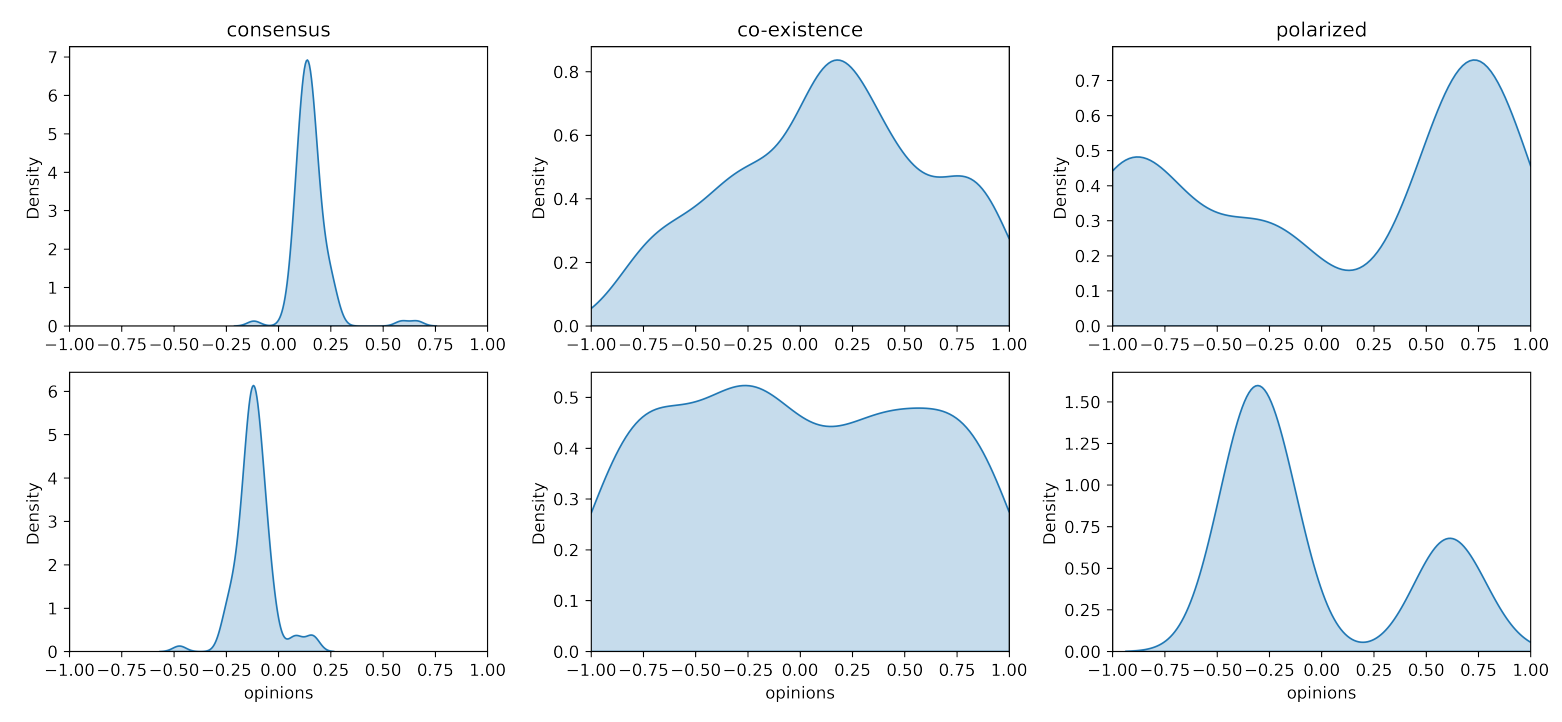
The distributions of Figure 4 are created by using a kernel density estimate with a bandwith of 0.9 (using the kde function from seaborn Waskom 2021). Next, we counted the peaks in the distributions using scipy’s find_peaks function (Virtanen et al. 2020). We ignore peaks that are smaller than 1/10 of the highest peaks, so for the distributions for the consensus state in Figure 4 this leads to one peak. Next, we set the prominence of a peak to 0.1, as to not count all minor ‘wiggles’ in the distribution, thus leading to one peak for the bottom distribution for the co-existence state in Figure 4. The distinction between the consensus and co-existence state was made based on their variance: If the variance of the distribution was smaller than 0.05, the network was considered as a consensus state, otherwise it was considered as a co-existence state network. These parameters were chosen such that the three states were identifiable.
Note: This way of counting the number of peaks performs poorly in providing exact number of peaks when that number is larger than 2 (i.e. the top distribution in the polarized state in Figure 4 counts two peaks, whereas Figure 1 clearly shows three clusters), but as the 3-cluster and 2-cluster networks are all in the polarized state, this is not influencing our results.
Appendix B: Verification of Individual Submodules
Module 1: Remove links
We run module 1 in isolation by setting \(tries\_createlink\), \(tries\_valuechange\), and \(tries\_opinionchange\) to 0. In this situation we expect that the only dynamics we observe is the removal of links of neighbors with an opinion that differs more than \(dist\_removelink\). To test this effect, we set \(dist\_removelink\) to 0.6 and to 0.25. The first one is the default value in future simulations, the latter is an extreme value to see the effect in an extreme case. Agents are never allowed to become completely disconnected, i.e. everybody should in the end still be connected to at least one other agent. This module behaves as expected, as the only process we observe is the removal of links (Figure 5).
Module 2: Create links
We run module 2 in isolation by setting \(prob\_removelink\), \(tries\_valuechange\), and \(tries\_opinionchange\) to 0. In this situation we expect that the only observed dynamics are the creation of new links between agents with an opinion that differs no more than \(dist\_createlink\). To explore this effect, we set \(dist\_createlink\) to 0.1 and to 0.8. The first one is the default value in future simulations, the latter is an extreme value to observe the effect of an extreme case. Agents should never have more neighbors than \(maxnb\) which is set at 10 in the default case and to 20 in the extreme case. The module behaves as expected, as the only process we observe is the creation of links (Figure 6).
Module 3: Update values
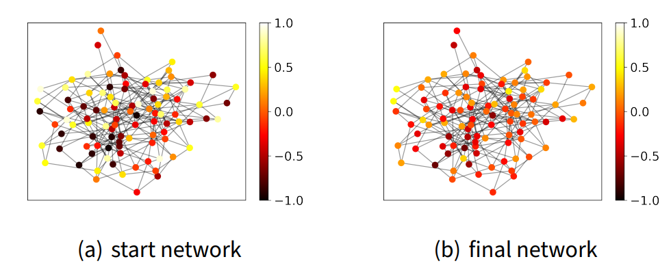
We run module 3 in isolation by setting \(tries\_createlink\), \(prob\_removelink\), and \(tries\_opinionchange\) to 0. In this situation we expect that the only process we observe is that the values of agents converge, as all agents adapt their values to be more in line with their neighbors. The network should not change, since no links are formed or removed. We explore this behaviour in a network of 100 agents. The module behaves as expected, as the links remain unchanged and the values converge towards each other (Figure 7).
Module 4: Update opinions
We run module 4 in isolation by setting \(tries\_createlink\), \(prob\_removelink\), and \(tries\_valuechange\) to 0. In this situation, we expect the opinions to converge towards each other, if the temperature is suffiently low, stubborness is sufficiently low and persuasiveness is sufficiently high. Therefore, we explore this mechanism by first setting \(T = 0.1\), \(stubbornness = 0\) for all agents and \(persuasiveness = 1\) for all agents. Next we test extreme values of these three parameters one factor at a time. Additionally, we explore the combined effect of stubbornness and persuasiveness.
In the default situation, all opinions converge towards each other over time (Figure 8a). If we increase the temperature \(T\) to 10, the opinions should remain random (i.e. people update their opinion every time without taking their neighbors opinions into account) (Figure 8b). If we implement cognitive dissonance by setting \(dist\_cd = 1\) we observe stronger deviations away from the average opinion, as expected, since agents update their opinion away from neighbors with a different value (Figure 8c). To explore the effects of stubbornness, we set the stubbornness of 50 random agents to 1, to ensure the existence of several stubborn agents in our network. Here, we expect that these 50 agents will not change their opinion, their extreme opinion might create little bubbles around them as they can still influence their (unstubborn) neighbors. This is indeed what we observe in Figure 8 d. To explore the effect of persuasiveness, we set the persuasiveness of 50 random agents to 0, to ensure the existence of some agents without any persuasiveness, i.e. whose opinion is not shared within the network. We expect slower convergence. If there is an agent whose only neighbor is an unpersuasive one, this agent will not be able to change its opinion. This is indeed what we observe in Figure 8e. Last, we explore the combined effects of stubbornness and persuasiveness. Here we expect little difference with the previous two scenarios, although more deviations away from the average opinion are possible due to variations in stubbornness and persuasiveness. Also these synergies of the module behave as expected (Figure 8f).
Appendix C: Pairwise Plots Visualizing Parameter Interactions
Appendix D: Exploring 3D Interactions
Appendix E: Exploring Mechanisms Behind the \(dist\_removelink\) OFAT
References
ADAMS, J. A., White, G., & Araujo, R. P. (2021). The role of mistrust in the modelling of opinion adoption. Journal of Artificial Societies and Social Simulation, 24(4), 4. [doi:10.18564/jasss.4624]
ALKEMADE, F., & Coninck, H. de. (2021). Policy mixes for sustainability transitions must embrace system dynamics. Environmental Innovation and Societal Transitions, 41, 24–26. [doi:10.1016/j.eist.2021.10.014]
ARROW, K. J. (1950). A difficulty in the concept of social welfare. Journal of Political Economy, 58(4), 328–346. [doi:10.1086/256963]
BALENZUELA, P., Pinasco, J. P., & Semeshenko, V. (2015). The undecided have the key: Interaction-driven opinion dynamics in a three state model. PLoS One, 10(10), e0139572. [doi:10.1371/journal.pone.0139572]
BARON, J. W. (2021). Consensus, polarization, and coexistence in a continuous opinion dynamics model with quenched disorder. Physical Review E, 104(4), 044309. [doi:10.1103/physreve.104.044309]
BOGUEVA, D., Marinova, D., & Gordon, R. (2020). Who needs to solve the vegetarian men dilemma? Journal of Human Behavior in the Social Environment, 30(1), 28–53. [doi:10.1080/10911359.2019.1664966]
BREETZ, H. L., Fisher-Vanden, K., Jacobs, H., & Schary, C. (2005). Trust and communication: Mechanisms for increasing farmers’ participation in water quality trading. Land Economics, 81(2), 170–190. [doi:10.3368/le.81.2.170]
CASTELLANO, C., Fortunato, S., & Loreto, V. (2009). Statistical physics of social dynamics. Reviews of Modern Physics, 81(2), 591. [doi:10.1103/revmodphys.81.591]
COUZIN, I. D., Krause, J., Franks, N. R., & Levin, S. A. (2005). Effective leadership and decision-making in animal groups on the move. Nature, 433(7025), 513–516. [doi:10.1038/nature03236]
DEFFUANT, G., Amblard, F., Weisbuch, G., & Faure, T. (2002). How can extremism prevail? A study based on the relative agreement interaction model. Journal of Artificial Societies and Social Simulation, 5(4), 1.
DEFFUANT, G., Neau, D., Amblard, F., & Weisbuch, G. (2001). Mixing beliefs among interacting agents. Advances in Complex Systems, 3(01n04), 87–98. [doi:10.1142/s0219525900000078]
DEGROOT, M. H. (1974). Reaching a consensus. Journal of the American Statistical Association, 69(345), 118–121. [doi:10.1080/01621459.1974.10480137]
DUNBAR, R. (2010). How Many Friends Does One Person Need? Dunbar’S Number and Other Evolutionary Quirks. Cambridge, MA: Harvard University Press. [doi:10.2307/j.ctvk12rgx]
EBRAHIMI, O. V., Johnson, M. S., Ebling, S., Amundsen, O. M., Hals, Ø., Hoffart, A., Skjerdingstad, N., & Johnson, S. U. (2021). Risk, trust, and flawed assumptions: Vaccine hesitancy during the COVID-19 pandemic. Frontiers in Public Health, 9, 849. [doi:10.3389/fpubh.2021.700213]
EDMONDS, B., Le Page, C., Bithell, M., Chattoe-Brown, E., Grimm, V., Meyer, R., Montañola-Sales, C., Ormerod, P., Root, H., & Squazzoni, F. (2019). Different modelling purposes. Journal of Artificial Societies and Social Simulation, 22(3), 6. [doi:10.18564/jasss.3993]
EKER, S., Reese, G., & Obersteiner, M. (2019). Modelling the drivers of a widespread shift to sustainable diets. Nature Sustainability, 2(8), 725–735. [doi:10.1038/s41893-019-0331-1]
FELDMANHALL, O., & Shenhav, A. (2019). Resolving uncertainty in a social world. Nature Human Behaviour, 3(5), 426–435. [doi:10.1038/s41562-019-0590-x]
FESTINGER, L. (1962). Cognitive dissonance. Scientific American, 207(4), 93–106. [doi:10.1038/scientificamerican1062-93]
FILATOVA, T., Verburg, P. H., Parker, D. C., & Stannard, C. A. (2013). Spatial agent-based models for socio-ecological systems: Challenges and prospects. Environmental Modelling & Software, 45, 1–7. [doi:10.1016/j.envsoft.2013.03.017]
FLACHE, A., Mäs, M., Feliciani, T., Chattoe-Brown, E., Deffuant, G., Huet, S., & Lorenz, J. (2017). Models of social influence: Towards the next frontiers. Journal of Artificial Societies and Social Simulation, 20(4), 2. [doi:10.18564/jasss.3521]
FULTON, E. A., Smith, A. D., Smith, D. C., & Putten, I. E. van. (2011). Human behaviour: The key source of uncertainty in fisheries management. Fish and Fisheries, 12(1), 2–17. [doi:10.1111/j.1467-2979.2010.00371.x]
FUNG, K. (2003). The significance of initial conditions in simulations. Journal of Artificial Societies and Social Simulation, 6(3), 9.
GARCIA, D., Galaz, V., & Daume, S. (2019). EATLancet vs yes2meat: The digital backlash to the planetary health diet. The Lancet, 394(10215), 2153–2154. [doi:10.1016/s0140-6736(19)32526-7]
GASTNER, M. T., Takács, K., Gulyás, M., Szvetelszky, Z., & Oborny, B. (2019). The impact of hypocrisy on opinion formation: A dynamic model. PLoS One, 14(6), e0218729. [doi:10.1371/journal.pone.0218729]
GRIMM, V., Berger, U., Bastiansen, F., Eliassen, S., Ginot, V., Giske, J., Goss-Custard, J., Grand, T., Heinz, S. K., Huse, G., Huth, A., Jepsen, J. U., JNørgensen, C., Mooij, W. M., Müller, B., Pe’er, G., Piou, C., Railsback, S. F., Robbins, A. M., … DeAngelis, D. L. (2006). A standard protocol for describing individual-based and agent-based models. Ecological Modelling, 198(1), 115–126. [doi:10.1016/j.ecolmodel.2006.04.023]
GRIMM, V., Berger, U., DeAngelis, D. L., Polhill, J. G., Giske, J., & Railsback, S. F. (2010). The ODD protocol: A review and first update. Ecological Modelling, 221(23), 2760–2768. [doi:10.1016/j.ecolmodel.2010.08.019]
HEGSELMANN, R. (2004). Opinion dynamics: Insights by radically simplifying models. In D. Gillies (Ed.), Laws and Models in Science (pp. 1–29). London: Kings College.
HEGSELMANN, R., & Krause, U. (2002). Opinion dynamics and bounded confidence models, analysis, and simulation. Journal of Artificial Societies and Social Simulation, 5(3), 2.
HEGSELMANN, R., & Krause, U. (2005). Opinion dynamics driven by various ways of averaging. Computational Economics, 25(4), 381–405. [doi:10.1007/s10614-005-6296-3]
HERMAN, J., & Usher, W. (2017). SALib: An open-source Python library for sensitivity analysis. Journal of Open Source Software, 2(9). [doi:10.21105/joss.00097]
HERMANS, R. C., Lichtwarck-Aschoff, A., Bevelander, K. E., Herman, C. P., Larsen, J. K., & Engels, R. C. (2012). Mimicry of food intake: The dynamic interplay between eating companions. PLoS One, 7(2), e31027. [doi:10.1371/journal.pone.0031027]
HUET, S., & Deffuant, G. (2010). Openness leads to opinion stability and narrowness to volatility. Advances in Complex Systems, 13(03), 405–423. [doi:10.1142/s0219525910002633]
JAGER, W., & Amblard, F. (2005). Uniformity, bipolarization and pluriformity captured as generic stylized behavior with an agent-based simulation model of attitude change. Computational & Mathematical Organization Theory, 10(4), 295–303. [doi:10.1007/s10588-005-6282-2]
JOHNSON, N. F., Velásquez, N., Restrepo, N. J., Leahy, R., Gabriel, N., El Oud, S., Zheng, M., Manrique, P., Wuchty, S., & Lupu, Y. (2020). The online competition between pro-and anti-vaccination views. Nature, 582(7811), 230–233. [doi:10.1038/s41586-020-2281-1]
KATERELOS, I. D., & Koulouris, A. (2004). Seeking equilibrium leads to chaos: Multiple equilibria regulation model. Journal of Artificial Societies and Social Simulation, 7(2), 4.
KEMPER, J. A., & White, S. K. (2021). Young adults’ experiences with flexitarianism: The 4Cs. Appetite, 160, 105073. [doi:10.1016/j.appet.2020.105073]
KWAKKEL, J. H. (2017). The exploratory modeling workbench: An open source toolkit for exploratory modeling, scenario discovery, and (multi-objective) robust decision making. Environmental Modelling & Software, 96, 239–250. [doi:10.1016/j.envsoft.2017.06.054]
LIBRE, S. V., van Voorn, G. A., ten Broeke, G. A., Bailey, M., Berentsen, P., & Bush, S. R. (2015). Effects of social factors on fishing effort: The case of the Philippine tuna purse seine fishery. Fisheries Research, 172, 250–260. [doi:10.1016/j.fishres.2015.07.033]
MACY, M. W., Kitts, J. A., Flache, A., & Benard, S. (2003). Polarization in dynamic networks: A Hopfield model of emergent structure. In R. Breiger, K. Carley, & P. Pattison (Eds.), Dynamic Social Network Modeling and Analysis (pp. 162–173). Washington, DC: The National Academies Press.
MCKAY, M. D. (1992). Latin hypercube sampling as a tool in uncertainty analysis of computer models. [doi:10.1145/167293.167637]
MINH Pham, T., Kondor, I., Hanel, R., & Thurner, S. (2020). The effect of social balance on social fragmentation. Journal of the Royal Society Interface, 17(172), 20200752. [doi:10.1098/rsif.2020.0752]
PIANOSI, F., & Wagener, T. (2018). Distribution-based sensitivity analysis from a generic input-output sample. Environmental Modelling & Software, 108, 197–207. [doi:10.1016/j.envsoft.2018.07.019]
SALZARULO, L. (2006). A continuous opinion dynamics model based on the principle of meta-contrast. Journal of Artificial Societies and Social Simulation, 9(1), 13.
SARRAZIN, F., Pianosi, F., & Wagener, T. (2016). Global sensitivity analysis of environmental models: Convergence and validation. Environmental Modelling & Software, 79, 135–152. [doi:10.1016/j.envsoft.2016.02.005]
SCHLUETER, M., Mcallister, R. R., Arlinghaus, R., Bunnefeld, N., Eisenack, K., Hoelker, F., Milner-Gulland, E. J., Müller, B., Nicholson, E., Quaas, M., & others. (2012). New horizons for managing the environment: A review of coupled social-ecological systems modeling. Natural Resource Modeling, 25(1), 219–272.
SCHNEIDER, A., & Ingram, H. (1990). Behavioral assumptions of policy tools. The Journal of Politics, 52(2), 510–529. [doi:10.2307/2131904]
SCHWARTZ, S. H. (1994). Are there universal aspects in the structure and contents of human values? Journal of Social Issues, 50(4), 19–45. [doi:10.1111/j.1540-4560.1994.tb01196.x]
TEN Broeke, G., van Voorn, G., & LigTENberg, A. (2016). Which sensitivity analysis method should I use for my agent-based model? Journal of Artificial Societies and Social Simulation, 19(1), 5. [doi:10.18564/jasss.2857]
VAN Voorn, G., Hengeveld, G., & Verhagen, J. (2020). An agent based model representation to assess resilience and efficiency of food supply chains. PLoS One, 15(11), e0242323. [doi:10.1371/journal.pone.0242323]
VAN Voorn, G., Ligtenberg, A., & ten Broeke, G. (2014). A spatially explicit agent-based model of opinion and reputation dynamics. Proceedings of the Social Simulation Conference, Barcelona, Spain [doi:10.18564/jasss.2857]
VIRTANEN, P., Gommers, R., Oliphant, T. E., Haberland, M., Reddy, T., Cournapeau, D., Burovski, E., Peterson, P., Weckesser, W., Bright, J., van der Walt, S. J., Brett, M., Wilson, J., Millman, K. J., Mayorov, N., Nelson, A. R. J., Jones, E., Kern, R., Larson, E., … SciPy 1.0 Contributors. (2020). SciPy 1.0: Fundamental Algorithms for Scientific Computing in Python. Nature Methods, 17, 261–272. [doi:10.1038/s41592-020-0772-5]
WASKOM, M. L. (2021). seaborn: Statistical data visualization. Journal of Open Source Software, 6(60), 3021. [doi:10.21105/joss.03021]
WEBB, P., Benton, T. G., Beddington, J., Flynn, D., Kelly, N. M., & Thomas, S. M. (2020). The urgency of food system transformation is now irrefutable. Nature Food, 1(10), 584–585. [doi:10.1038/s43016-020-00161-0]
WILLETT, W., Rockström, J., Loken, B., Springmann, M., Lang, T., Vermeulen, S., Garnett, T., Tilman, D., DeClerck, F., Wood, A., & others. (2019). Food in the Anthropocene: The EAT-Lancet Commission on healthy diets from sustainable food systems. The Lancet, 393(10170), 447–492. [doi:10.1016/s0140-6736(18)31788-4]
WU, T. T., McCoy, B. M., Tracy, C. A., & Barouch, E. (1976). Spin-spin correlation functions for the two-dimensional Ising model: Exact theory in the scaling region. Physical Review B, 13(1), 316. [doi:10.1103/physrevb.13.316]
YILDIZ, E., Ozdaglar, A., Acemoglu, D., Saberi, A., & Scaglione, A. (2013). Binary opinion dynamics with stubborn agents. ACM Transactions on Economics and Computation (TEAC), 1(4), 1–30. [doi:10.1145/2538508]
ZALLER, J. (1991). Information, values, and opinion. American Political Science Review, 85(4), 1215–1237. [doi:10.2307/1963943]