Explaining “U-Shaped” Distributions of Population Substance Use with a Simple Computational Approach

aDartmouth Geisel School of Medicine, Dartmouth College, United States
Journal of Artificial
Societies and Social Simulation 28 (2) 5![]()
<https://www.jasss.org/28/2/5.html>
DOI: 10.18564/jasss.5586
Received: 17-Nov-2023 Accepted: 14-Mar-2025 Published: 31-Mar-2025
Abstract
Background: “U-shaped” distributions of past 30-day substance use frequencies are pervasive, yet no established model explains this phenomenon. Using probability functions to describe these distributions yields unintuitive, atheoretical results. This study introduces a simple computational model of individual-level, longitudinal substance use patterns to understand how cross-sectional U-shaped distributions emerge in populations. Model: Each independent computational object transitions between two states: not using a substance (“N”), or using a substance (“U”). The model has two key components: (1) each object has a unique risk factor probability governing the transition from N to U, and a unique protective factor probability governing the transition from U to N; (2) an object’s current decision to use or not use is influenced by its prior decisions (i.e., “path dependence”). Three modeler input parameters control these two components. Analysis: First, the model is fit to empirical cross-sectional distributions of past 30-day use frequencies for ten substances (e.g., alcohol, cannabis, tobacco, etc.) from the U.S. National Survey on Drug Use and Health. Next, combinations of values of the model’s three inputs are tested to determine the conditions that produce U-shaped distributions. Finally, supplemental testing explored structural variations of the original model to assess whether simpler or alternative configurations are also capable of generating U-shaped distributions. Results: The model effectively reproduced the U-shaped distributions observed in empirical data across all substances. Path dependence emerged as a critical feature for generating U-shaped distributions, independent of the specific distribution shapes used for assigning transition probabilities. However, results also indicated that neither of the model's two key components are required for generating U-shaped distributions. Conclusion: This study demonstrates how a simple, theoretically-grounded computational model of individual-level substance use patterns can help substance use researchers understand the emergence of population-level, cross-sectional U-shaped distributions of substance use.Introduction
Each year, the National Survey on Drug Use and Health (NSDUH) surveys a random cross-section of the U.S. population to measure substance use patterns by asking questions such as, "During the past 30 days, on how many days did you use marijuana or hashish?" and "During the past 30 days, on how many days did you drink one or more drinks of an alcoholic beverage?"(Center for Behavioral Health Statistics and Quality 2020a). Regardless of the substance (e.g., alcohol, cannabis, tobacco, opioids, stimulants, etc.), the distribution of responses to these questions is almost invariably “U-shaped” with many low-frequency consumers, many daily consumers, and fewer in between.
The field of substance use epidemiology lacks a coherent model to explain how this U-shaped phenomenon occurs. This may be due in part to the limitations of traditional statistical approaches and perspectives on the purpose of scientific models. For example, part of a typical phenomenologically-oriented (Porgo et al. 2019) approach to modeling a U-shaped distribution might be to fit a Beta distribution to estimate values for the two parameters that govern the shape of the distribution (Burgette et al. 2021; Wagner et al. 2015). This modeling approach has four major limitations: (1) It reifies probability functions by assuming such functions are the literal data-generating mechanisms of natural phenomena rather than treating them more appropriately as atheoretical mathematical summaries of the output of underlying processes; (2) Consequently, a primary aim of standard statistical approaches is to describe – rather than explain – the shape of a distribution. Although statistical descriptions (e.g., values for alpha and beta parameters in a Beta distribution) are useful for cross-sectional prediction models, they do not provide plausible explanations for the underlying processes that generate the behavior of interest (e.g., substance use), nor are they particularly useful for understanding how these behaviors might evolve over time; (3) The equations used to describe the distribution are often non-intuitive; (4) Different substances (e.g., tobacco, cannabis, alcohol, opioids) may require different families of probability distributions.
Instead of creating an uninterpretable statistical description, we can develop a generalized explanation of how the U-shaped distribution phenomenon occurs by testing whether a theoretically-grounded micro-level process (e.g., individual-level, data-generating mechanism of longitudinal substance use decision sequences) plausibly governs the observed macro-level phenomenon (e.g., population-level, cross-sectional U-shaped distributions of substance use)(Li & O’Donoghue 2012; Spielauer 2011).
The goal of this study was to develop a simple computational model to explain empirical U-shaped distributions of population substance use. Specifically, this study: (1) Presents a simple computational model that generates individual-level longitudinal sequences of decisions to use or not use a substance; (2) Determines whether these individual-level sequences can accurately reproduce the empirical cross-sectional U-shaped population distributions of past 30-day consumption frequencies in the US for multiple psychoactive substances; (3) Probes the model’s components and assumptions to understand how they contribute to the model’s output.
Methods
This study “…makes a simulation in which certain mechanisms or processes are built in …” to determine if “…the outcomes of the simulation match some (known) data …” and thereby “…support an explanation of the data using the built-in mechanisms”(Edmonds et al. 2019). The model is outlined using a mix of several guidelines (Grimm et al. 2006, 2020; Hammond 2015; Wilson & Collins 2019). The study was conducted using Python 3.11 and Stata 18. All simulation results were obtained using at least 20,000 objects. The Python code for the model is archived in the CoMSES Model Library: https://www.comses.net/codebase-release/6b188c71-3bd7-4ae4-85f0-eb9c68668630/. This study was deemed exempt from review by the Dartmouth Committee for the Protection of Human Subjects.
Model overview
This model uses a two-state, path-dependent, discrete stochastic process to generate multiple individual-level sequences of substance use patterns (i.e., longitudinal data) to reproduce the cross-sectional distributions of past 30-day substance use frequencies observed in the U.S. National Survey on Drug Use and Health (NSDUH). The model is perhaps best classified as a simplified dynamic microsimulation. However, this study uses empirical data (NSDUH data) as the target when searching for optimal values of the model’s three input parameters (i.e., modeling the “inverse problem”). In contrast, “true” microsimulations often use empirical data (e.g., demographic census data) to calibrate the initial state of the model in order to forecast future outcomes (i.e., modeling the “forward problem”) (Klevmarken 2022; Li & O’Donoghue 2012, 2014; Ritter et al. 2016; Spielauer 2011; Tarantola 2023; van Imhoff & Post 1998).
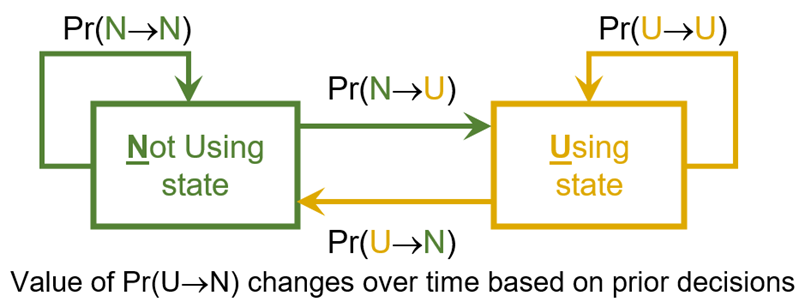
The model is populated with independent computational objects that do not interact directly or indirectly. At each step in time \(t\) (i.e., each "day"), each object decides whether to use (represented as 1) or not use (represented as 0) the substance. Each object generates a sequence of binary states – "Not using" (\(N\)) or "Using" (\(U\)) – representing its substance use over time. The model has two core components. Component 1. Each object is assigned two unique state transition probabilities: a “risk factors effect” probability of transitioning from \(N\) to \(U\), i.e., \(Pr(N \rightarrow U)\), and a “protective factors effect” probability of transitioning from \(U\) to \(N\), i.e., \(Pr(U \rightarrow N)\) (Figure 1, Table 1). Component 2. Path dependence: Similar to dynamic microsimulations (Spielauer 2011), the value of \(Pr(U \rightarrow N)\) changes based on the object’s history of decisions (i.e., path dependence) (Figure 1, Table 1, Equation 1). The modeler uses three input parameters (Table 2) to control these two components.
| Individual Object’s Decision Probabilities | Static or Dynamic Value | Calculation |
|---|---|---|
| Pr(N\(\rightarrow\)U) (i.e., “risk factor effect” transition probability) | Static | Random draw from risk factor distribution (uniform distribution) at model initialization |
| Pr(N\(\rightarrow\)N) | Static | 1 - Pr(N\(\rightarrow\)U) |
| Pr(U\(\rightarrow\)N) (i.e., “protective factor effect” transition probability) | Dynamic | Pr(U\(\rightarrow\)N)\(_{t=0}\) is a random draw from protective factor distribution (uniform distribution) at model initialization Pr(U\(\rightarrow\)N)\(_{t>0}\) = Pr(U\(\rightarrow\)N)\(_{t=0} \times\) \(e^{(-\text{proportion days used} \times \text{reinforcing effect})}\) |
| Pr(U\(\rightarrow\)U) | Dynamic | 1 - Pr(U\(\rightarrow\)N) |
| Notes: (1) \(t\) = time step; (2) proportion of days used calculated using 30 as the denominator; (3) value of Pr(U\(\rightarrow\)N)\(_{t>0}\) is re-calculated during each step that object is in the Using state. | ||
Rationale for the two core components of the model
Core component 1: Unique risk and protective factor effects (i.e., unique state transition probabilities)
Numerous biopsychosocial factors (e.g., genetics, family interactions, peer networks, socioeconomics, cultural and generational trends, etc.) influence substance use initiation, maintenance, and abstention (Galea et al. 2009; Rhodes et al. 2003; Sloboda et al. 2012; Stone et al. 2012). These factors are often divided into “risk factors” and “protective factors”. Risk factors are associated with a greater probability of substance use (e.g., family and peer substance use, impoverished neighborhood), and protective factors are associated with a decreased probability of substance use (e.g., high prices, social stigma, availability of healthy alternatives). Each object’s unique "risk factor effect" transition probability represents the aggregate effect of multiple risk factors, and its unique "protective factor effect" transition probability represents the aggregate effect of multiple protective factors. The distribution of these aggregate risk and protective factors is controlled by the modeler (discussed below; see Table 2). Note that computational models of substance use often explicitly incorporate specific (rather than aggregate) risk and protective factors (e.g., heroin subtypes, size of injection networks, etc.) to examine their interactions and provide insights into particular aspects of substance use dynamics (Bobashev et al. 2020). The decision to include such specific factors largely depends on the research questions and objectives.
Core component 2: Path dependence and Reinforcing Effect
Behavioral Science has established that the consequences (positive and negative) of a behavior will alter the probability of re-engaging in that behavior (Catania 2010). Humans and other organisms learn that certain behaviors (e.g., consuming a psychoactive substance) produce reinforcing consequences (e.g., pleasurable subjective feeling, social validation, increased work productivity, etc.) and subsequently seek to repeat the behaviors that produced the reinforcing consequences (Bickel et al. 2014; Panlilio & Goldberg 2007; Vollmer & Hackenberg 2001). As Epskamp and colleagues have noted, "Substance use behaviors are an example of a psychological system that exhibits feedback: the use of substances and the circumstances in which it takes place can impact one’s life in both the short-term and long-term, creating environments that are reinforcing thereby impacting the amount of substance use" (Epskamp et al. 2022). Consequently, the present model was programmed so that an object’s probability of current substance use is contingent on its historical patterns of substance use (i.e., path-dependent system) (David 2007; Turner & Baker 2019). The modeler controls the degree to which an object’s historical patterns of substance use affect the probability of current substance use by altering the input value of the Reinforcing Effect parameter (additional details discussed below).
Model design
Initialization and modeler input
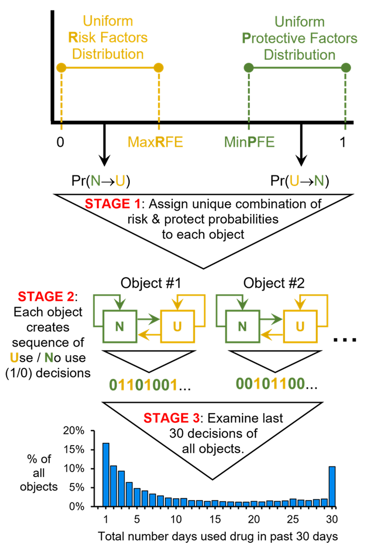
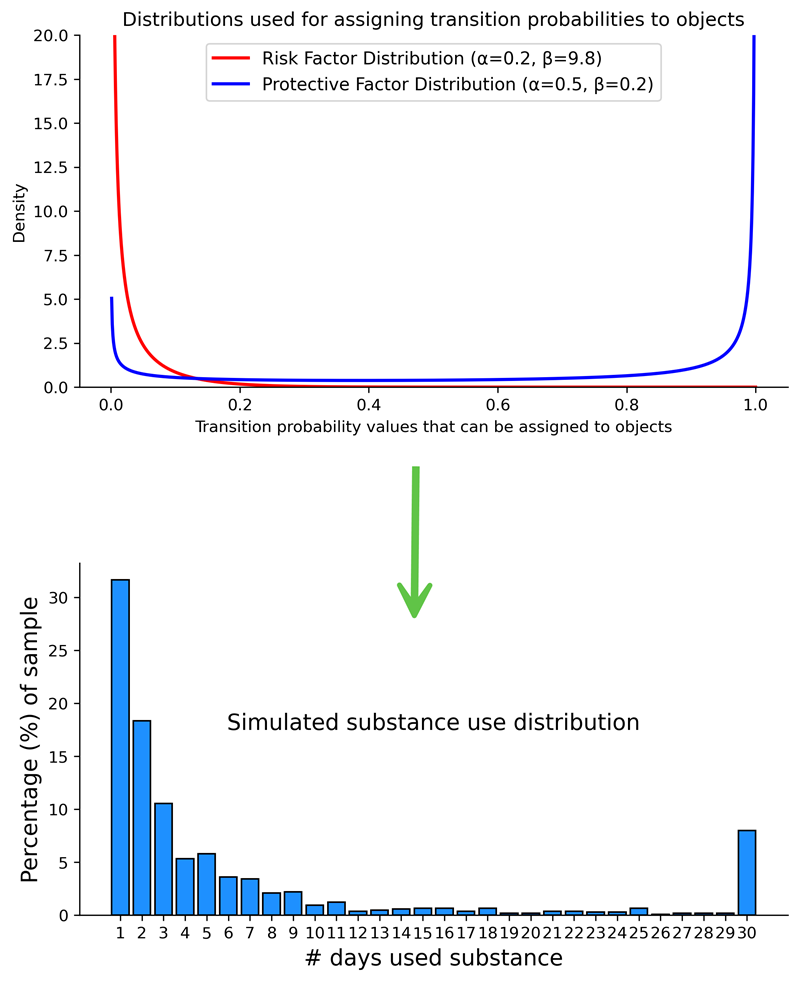
To initialize the model, the modeler set three parameters: (1) Maximum Risk Factors Effect (MaxRFE), (2) Minimum Protective Factors Effect (MinPFE), (3) Reinforcing Effect (RE). At \(t=0\), each object receives a unique “risk factors effect” by drawing from a uniform distribution bounded between zero (inclusive) and MaxRFE (i.e., drawing from the Risk Factors distribution). Each object also receives a unique "protective factors effect by drawing from a uniform distribution bounded between MinPFE and 1 (inclusive) (i.e., drawing from the Protective Factors distribution). The RE is a global, fixed value for all objects. Larger RE values introduce more path dependence. Of note, using a uniform distribution to assign risk and protective factor probabilities to objects does not imply that all objects have the same, homogeneous environment. On the contrary, using a uniform distribution ensures that transition probabilities are drawn from a wide range of potential values, which in turn, ensures that each object is assigned a unique combination of risk and protective probabilities to reflect a distinct theoretical biopsychosocial profile.
| Parameter | Description | Notes |
|---|---|---|
| Maximum Risk Factors Effect (“MaxRFE”) | Maximum possible value of Pr(N\(\rightarrow\)U) that can be assigned to a computational object. | \(0 < \text{MaxRFE} \leq 1\) |
| Minimum Protective Factors Effect (“MinPFE”) | Minimum possible value of Pr(U\(\rightarrow\)N) that can be assigned to a computational object. | \(0 \leq \text{MinPFE} < 1\) |
| Reinforcing Effect (“RE”) | Increasing reinforcing effect value will increase path dependence in the model. | \(\text{RE} > 0\) |
Object properties: "Using" state (\(U\)), "Not using" state (\(N\)), and transition probabilities
The Risk Factor distribution created by the modeler is used to assign each object a unique, fixed probability of transitioning from \(N\) to \(U\) called \(Pr(N \rightarrow U)\), which represents the object’s "Risk Factors Effect". \(Pr(N \rightarrow N)\) is the probability of remaining in the \(N\) state and is calculated as \(1 - Pr(N \rightarrow U)\). Each object also has a unique set of probabilities of transitioning from \(U\) to \(N\) called \(Pr(U \rightarrow N)\), which represents the object’s "Protective Factors Effect". \(Pr(U \rightarrow N)\) is initialized at \(t=0\) using the Protective Factor distribution created by the modeler and is denoted as \(Pr(U \rightarrow N)_{t = 0}\). However, as the simulation progresses, the value of \(Pr(U \rightarrow N)\) is adjusted based on the object’s recent history of substance use and the value of the RE parameter; this time step-specific value of \(Pr(U \rightarrow N)\) is denoted as \(Pr(U \rightarrow N)_{t > 0}\). Finally, \(Pr(U \rightarrow U)\) is the probability of remaining in the \(U\) state and is calculated as \(1 - Pr(U \rightarrow N)\).
Object action: determining current state and deciding to use or not use (Figure 2: Stage 2)
At the beginning of the current time step \(t\), each object determines whether it is in the \(N\) state or the \(U\) state by checking whether or not it used the substance in the prior step, \(t-1\). If the object did not use in the prior step, then it is in the \(N\) state at the beginning of the current step, and the probability that the object will use the substance during the current step is the object’s unique \(Pr(N \rightarrow U)\) value. If the object used the substance in the prior step, then it is in the \(U\) state at the beginning of the current step, and the probability that the object will not use the substance during the current step is the object’s time step-specific value of \(Pr(U \rightarrow N)\), i.e., \(Pr(U \rightarrow N)_{t > 0}\). By the end of step \(t\), the object decides whether or not to use the substance during step \(t\). If the object decides to use, it records a 1 in its personal use history; if the object decides not to use, it records a 0 in its personal use history.
Object action: updating the value of \(Pr(U \rightarrow N)\) (Figure 2: Stage 2)
If the object uses during the current time step, then the object’s \(Pr(U \rightarrow N)\) value is updated. This updated probability is termed \(Pr(U \rightarrow N)_{t > 0}\) and is used by the object in the subsequent time step \(t+1\) when deciding whether or not to use. The value of \(Pr(U \rightarrow N)_{t > 0}\) is calculated as:
| \[ Pr(U \rightarrow N)_{t > 0} = Pr(U \rightarrow N)_{t=0} \times e^{(-\text{proportion days used} \times \text{reinforcing effect})}\] | \[(1)\] |
Time, scheduling, and environment
A time step is completed after all computational objects have determined whether they use or not. Each time step is considered equivalent to one day after the model has stabilized (discussed below and in Appendix 1). There is no spatial component to the model.
Model evaluation
National Survey on Drug Use and Health (NSDUH)
The NSDUH is an annual, cross-sectional, multi-stage probability sample that assesses substance use behaviors among Americans age 12 and older with fixed household addresses (Center for Behavioral Health Statistics and Quality 2020a). NSDUH data can be used to estimate the proportion of the U.S. population who have engaged in a particular substance use behavior. The present analyses used combined NSDUH data (years 2002 to 2019; \(N=1,005,421\)) to examine past 30-day frequency of alcohol, cannabis, tobacco cigarette, heroin, prescription opioid, methamphetamine, cocaine and crack-cocaine, hallucinogen, inhalant, and tranquilizer use. Analyses for each substance were limited to NSDUH participants who had used the substance at least once in the past 30 days. For each substance, the proportion of past 30-day consumers who had used the substance on a given number of days was calculated and recorded (e.g., X% of past 30-day alcohol consumers had consumed alcohol on 9 days within the past 30 days) using the imputation-revised variables “iralcfm”, “irmjfm”, “ircigfm”, “irherfm”, “irpnrnm30fq”, “irmetham30n”, “ircocfm”, “ircrkfm”, “irhalluc30n”, “irinhal30n” “irtrqnm30fq”, and appropriate survey weighting procedures (Center for Behavioral Health Statistics and Quality 2020b).
Importantly, three modifications were made to the NSDUH data. First, the imputation-revised variables contained response values that were logically impossible for a discrete variable (e.g., used on 3.8 days). Therefore, values were rounded to the nearest integer. Second, empirical distributions of self-reported behaviors are often affected by the digit preference bias (Klesges et al. 1995; Wang & Heitjan 2008) (e.g., tendency to report consumption in denominations of five). Therefore, respondents who reported using on 5, 10, 15, 20, and 25 days were randomly assigned with equal probabilities to either their original response value, one day greater, or one day less. For example, those who reported using on 15 days in the past 30 days were randomly re-assigned to either 14, 15, or 16 days. Third, responses for cocaine and crack-cocaine were merged into a single variable by taking the respondent’s maximum reported usage days from the ‘ircocfm’ and ‘ircrkfm’ variables.
Model stability
Before the model could be used to simulate distributions of substance use, it was first necessary to determine the number of time steps required to obtain stable results. To determine the required number of time steps, simulated distributions were generated using different combinations of values of the three model input parameters: RE, MaxRFE, and MinPFE. During this process, the values of two of the three parameters were held constant while the value of the third parameter varied. For example, distributions were generated using RE parameter values of 3.0, 3.5, 4.0, 4.5, 5.0 while fixing the values of MaxRFE and MinPFE to 0.2 and 0.7, respectively. Each combination of parameter values was tested in a simulation using 100,000 objects and 2000 time steps. For each simulation, the number of daily (i.e., 30/30 days) consumers was divided by the number of once-per-month consumers at the end of each 100-step interval. A distribution was considered stable if this ratio no longer changed substantially (examined qualitatively). Sensitivity tests using different starting seeds were conducted. The results from these tests generally suggested that the model stabilized before reaching 1000 time steps. Therefore, a conservative 2000 time steps was chosen for the model evaluation process. Appendix 1 provides additional information and results.
Measuring edge value concentrations in distributions of past 30-day substance use frequencies
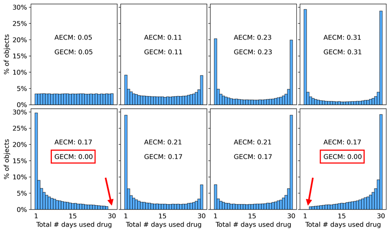
In analyses 2a and 2b, an Arithmetic Edge Concentration Measure (AECM; Equation 2) and Geometric Edge Concentration Measure (GECM; Equation 3) are used to quantify the “edge value concentration” of past 30-day substance use distributions. “Edge value concentration” refers to the extent to which a bounded distribution is dominated by edge values, i.e., the extent to which the data are concentrated near the minimum and maximum possible values. For example, a distribution of past 30-day substance use frequencies in which 40% used only one day and 40% used every day has high edge concentration and would yield high AECM and GECM values. The AECM and GECM are formally defined as:
| \[ AECM = \frac{E_{L} + E_{U}}{2}\] | \[(2)\] |
| \[ GECM = \sqrt{E_{L} \cdot E_{U}}\] | \[(3)\] |
| \[ E_L = \int_{L}^{L+\alpha(U-L)} f(x) \,dx\] | \[(4)\] |
| \[ E_U = \int_{U-\alpha(U-L)}^{U} f(x) \,dx\] | \[(5)\] |
Analysis 1: Fitting the model to NSDUH data to estimate optimal parameter values
For each of the ten substances, an ordinary least-squares (OLS) approach was used to identify the best fit between the proportions in a simulated distribution of past 30-day use frequencies (e.g., X% used on 1 day, Y% used on 2 days, etc) and the corresponding proportions in an empirical (NSDUH) distribution of past 30-day use frequencies. To sweep the parameter space, simulated distributions were generated using combinations of values for three parameters: MaxRFE, MinPFE, and RE (Appendix 2 provides additional details).
Analysis 2a: Determining how the model’s three inputs interact to generate U-shaped distributions
Analyses were conducted to understand how the three model inputs – MaxRFE, MinPFE, and RE – interact to generate U-shaped distributions. This analysis had two parts: illustrative and systematic. In the illustrative analysis, the optimized values of the three inputs (Table 3), and their corresponding simulated distributions were examined qualitatively to identify particular results that illustrate key explanatory interactions. Second, a systematic quantitative analysis explored how combinations of values for the three inputs affected the edge concentration (i.e., AECM and GECM values) of the simulated distributions. Specifically, analyses tested the 600 combinations from the Cartesian product of MaxRFE values from 0.1 to 1.0 in increments of 0.1; MinPFE values from 0.0 to 0.9 in increments of 0.1; and RE values of 0, 1, 2, 3, 4, and 5.
Analysis 2b: Using non-uniform distributions to assign risk and protective factor state transition probabilities
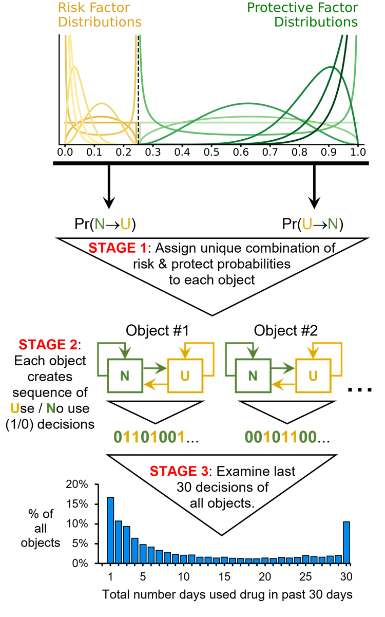
The model makes no assumptions about the distribution of its output (i.e., no assumptions about the shape of the resulting distribution of past 30-day substance use frequencies). However, the model does assume that the initial distributions used to assign risk and protective factor effects (i.e., initial distributions of transition probabilities \(Pr(N \rightarrow U)\) and \(Pr(U \rightarrow N)_{t = 0}\)) are uniform (see Figure 2: Stage 1). Therefore analyses were conducted to determine whether using non-uniform distributions to assign risk and protective factor transition probabilities \(Pr(N \rightarrow U)\) and \(Pr(U \rightarrow N)_{t = 0}\) to objects (Figure 4: Stage 1), impacted the model’s ability to generate U-shaped distributions (Figure 4: Stage 3). The analysis included seven starting distributions, six of which were non-uniform (a uniform distribution was included to contextualize results) (Figure 4: Stage 1). These shapes were chosen to encompass a wide range of plausible distributions in substance use research. The analysis used the 49 pairs from the Cartesian product of the seven distributions for assigning risk and protective probabilities. Each pair of distributions was tested at RE values of 0, 3, 4, and 5 – resulting in a total of 196 tests. A cutoff of 0.25 was used to create the non-uniform distributions such that the risk factor probability distribution ranged from 0.00 to 0.25, and the protective factor distribution ranged from 0.25 to 1.00 (Figure 4: Stage 1). This 0.25 cutoff was chosen because it roughly approximated the optimal MaxRFE and MinPFE cutoffs identified when the original model was fit to the empirical NSDUH data (see Table 3).
Analysis 3: Supplemental tests of alternative model designs (Appendix 3)
Supplemental analyses were conducted to further understand how specific assumptions and components of the original model influence the distributions it produces. The first set of tests (see “Supplemental Testing 1” below) examined the impact of assumptions about the relationship between \(Pr(N \rightarrow U)\) and \(Pr(U \rightarrow N)_{t = 0}\). The second set of analyses (see “Supplemental Testing 2” below) removed path dependence from the model but used a U-shaped distribution to assign initial transition probabilities to objects.
Supplemental Testing 1: Complementary Transition Probabilities (CTP) Model. In the original model, each object is assigned two independent state transition probabilities: \(Pr(N \rightarrow U)\) and \(Pr(U \rightarrow N)_{t = 0}\). These probabilities are independently drawn from uniform distributions, with \(Pr(N \rightarrow U)\) ranging from zero to MaxRFE, and \(Pr(U \rightarrow N)_{t = 0}\) ranging from MinPFE to one. This setup requires the modeler to specify two parameters: a MaxRFE value and a MinPFE value. To determine whether simpler models could also generate U-shaped distributions, a CTP version was tested. In the CTP model, each object’s \(Pr(N \rightarrow U)\) is still drawn from a uniform distribution ranging from zero to MaxRFE, but \(Pr(U \rightarrow N)_{t = 0}\) is automatically calculated as \(1 - Pr(N \rightarrow U)\). Note that this CTP model still used the path dependence function (Equation 1).
Supplemental Testing 2: Models with U-shaped initialization distributions but no path dependence. A second set of supplemental analyses evaluated whether models without path dependence (i.e., memoryless Markov models) could generate U-shaped distributions by assigning initial risk and protective transition probabilities that are concentrated near 0 and 1. In Supplemental Testing 2.1., \(Pr(N \rightarrow U)\) values were assigned using either narrow uniform distributions with means near zero or highly right-skewed distributions with means near zero, while \(Pr(U \rightarrow N)_{t = 0}\) values were assigned using either narrow uniform distributions with means near one or highly left-skewed distributions with means near one. In Supplemental Testing 2.2. \(Pr(N \rightarrow U)\) values were assigned using a highly right-skewed distribution with a mean near zero, and \(Pr(U \rightarrow N)_{t = 0}\) values were assigned using a U-shaped distribution with upward tails near both zero and one. Note that these alternative models still assigned two unique and uncorrelated transition probabilities to each object.
Results
Analysis 1 results: Fitting the model to NSDUH data
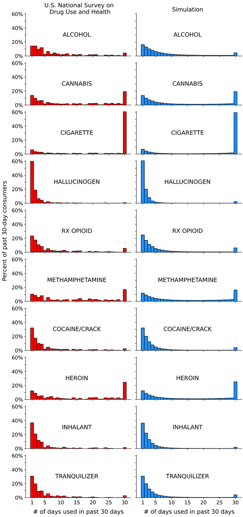
The left side of Figure 5 displays the NSDUH-based past 30-day use frequency distributions for each substance. The right side of Figure 5 displays the corresponding simulated distributions produced by the OLS-optimized values of MaxRFE, MinPFE, and RE (Table 3). The most important results to compare in Figure 5 and Table 3 are tobacco cigarettes, hallucinogens, and alcohol. Note that (1) the cigarette and hallucinogen distributions are “opposite” shapes; (2) cigarettes and hallucinogens both have high RE values, but very different MinPFE and MaxRFE values; (3) cigarettes and alcohol both have relatively low MinPFE values and similarly elevated MaxRFE values, but very different RE values.
| Substance | MaxRFE | MinPFE | RE |
|---|---|---|---|
| Alcohol | 0.16 | 0.54 | 3.1 |
| Cannabis | 0.17 | 0.57 | 3.8 |
| Tobacco Cigarette | 0.17 | 0.22 | 4.6 |
| Hallucinogen | 0.04 | 0.94 | 4.9 |
| Rx Opioid | 0.10 | 0.50 | 3.5 |
| Methamphetamine | 0.21 | 0.63 | 3.6 |
| Cocaine/Crack | 0.10 | 0.89 | 4.0 |
| Heroin | 0.17 | 0.50 | 3.9 |
| Inhalant | 0.09 | 0.91 | 3.9 |
| Tranquilizer | 0.10 | 0.82 | 3.9 |
Analysis 2a results: determining how the model’s three inputs (MaxRFE, MinPFE, RE) interact to generate U-shaped distributions
Association between edge concentration and RE values
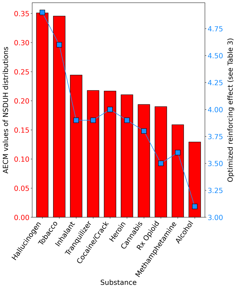
Figure 6 displays the relationship between the AECM values derived from the NSDUH distributions (see Figure 5) and the optimized RE value from the corresponding simulation (Table 3). In Figure 6, higher AECM values indicate that a greater total proportion of a substance’s frequency-of-use distribution is concentrated at the edges of that distribution and away from the middle of the distribution. For example, Hallucinogens and Tobacco had the largest AECM values – indicating that these two substances had the greatest total proportion of past 30-day consumers with extremely low use frequencies (e.g., once per month) and extremely high use frequencies (e.g., every day). The key takeaway from Figure 6 is that past 30-day substance use frequency distributions with high AECM values, such as tobacco and hallucinogens, required a high RE value, whereas distributions with lower AECM values (i.e., more evenly spread distributions), such as alcohol, required a lower RE value.
Interactions among RE, MaxRFE and MinPFE
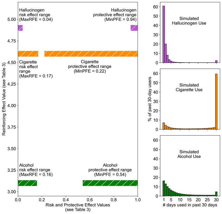
Using tobacco cigarettes, hallucinogens, and alcohol as examples, Figure 7 demonstrates how the three model inputs (RE, MaxRFE, MinPFE) interact to generate different types of U-shaped distributions. In the left graph of Figure 7, the x-axis length of colored bars indicates the optimal range of protective factor or risk factor probabilities identified for each substance (corresponds to Table 3 values). The y-axis location of each pair of colored bars indicates the optimal RE identified for each substance (corresponds to Table 3 values). The three subgraphs on the right side of Figure 7 display the simulated distributions corresponding to the model input values represented by the bar graphs (same distributions as those on right side of Figure 5). There are two key features to note about Figure 7. First, cigarettes and hallucinogens required similar RE values (i.e., similar y-axis values) but cigarettes required a much wider range of risk and protective factor effect probabilities (i.e., wider range of x-axis values). Having similar RE values, but dissimilar risk and protective factor ranges produces the “opposite” or “flipped” orientations of the cigarette and hallucinogen distributions. Second, the gradually sloping alcohol distribution required relatively wide ranges of risk factor and protective factor probabilities (similar to cigarettes) but also a low RE value (unlike cigarettes) to reduce path dependence in the model, and thereby reduce the number of daily consumers.
Systematic testing: Model input combinations and edge value concentrations of the resulting distributions
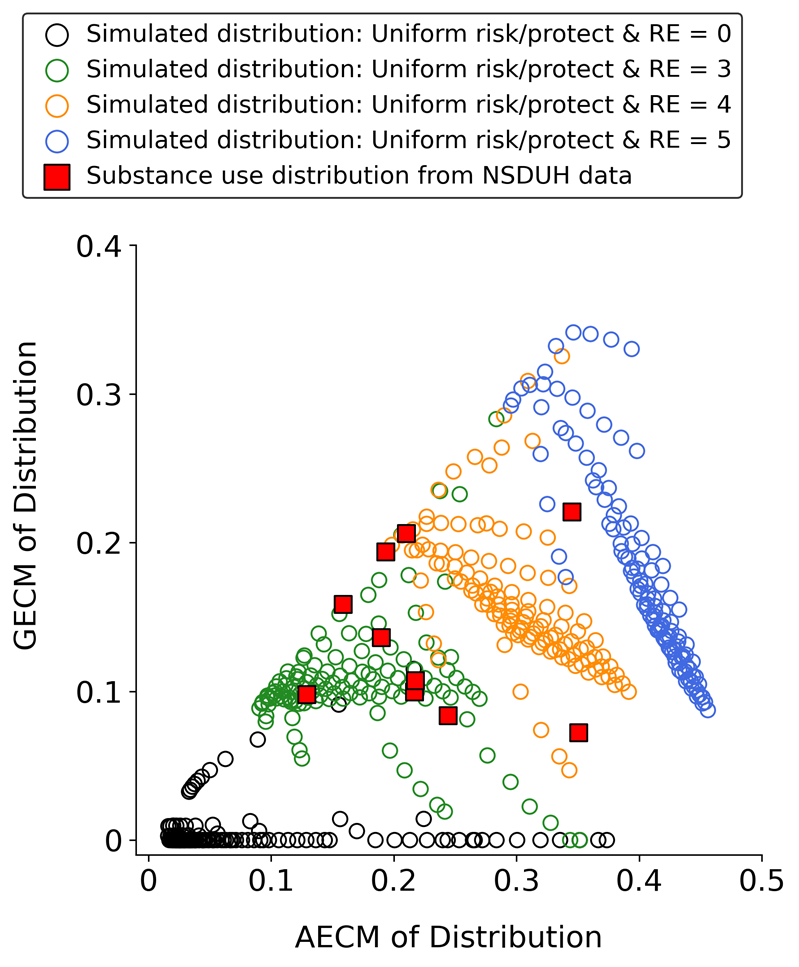
Figure 8 displays the AECM (green) and GECM (purple) values of the simulated substance use distributions produced by each of the 600 tested combinations of MaxRFE, MinPFE, and RE values. Darker colors indicate larger AECM and GECM values (i.e., greater concentration of data at the edges of a distribution). The right-most column displays example histograms to help contextualize the AECM and GECM values shown in the heatmap. Figure 8 shows that when the RE is set to a larger value (i.e., moving from an upper matrix to a lower matrix) the AECM and GECM values generally increase. Note that when the RE equals zero (i.e., no path dependence), the GECM values are also zero for the vast majority of cases – indicating that these distributions are not U-shaped. Figure 8 also suggests that the relationship between the MaxRFE, MinPFE, and RE parameters is a complex 3-way interaction. For example, the magnitude and direction (positive/negative) of the association between MinPFE values and GECM values depends on the RE and MaxRFE values. Similarly, the magnitude and direction of the association between MaxRFE values and GECM values depend on the RE and MinPFE values.
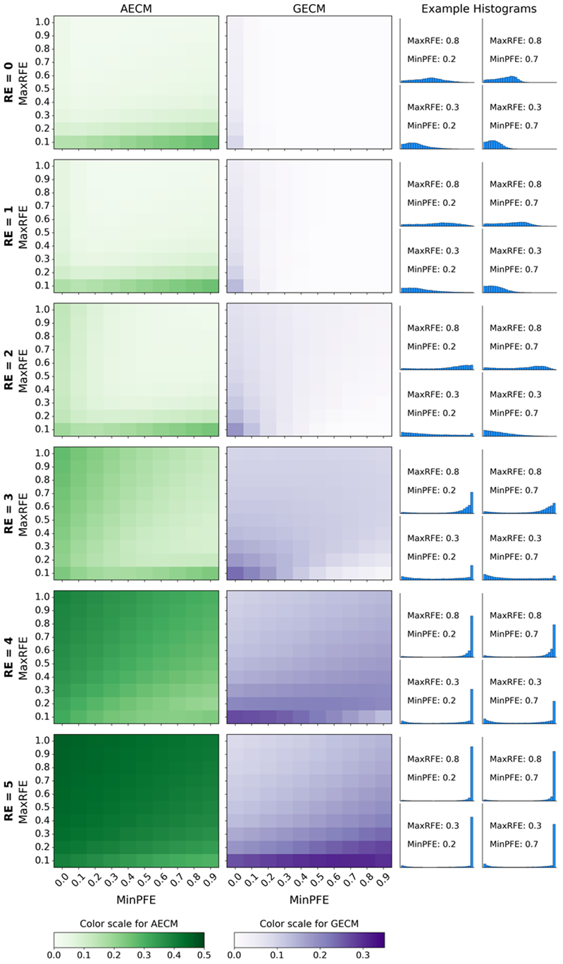
Figure 9 is a different way of displaying the same results in Figure 8. However, Figure 9 also includes the AECM and GECM values of the empirical NSDUH distributions to contextualize the accuracy of the simulated results. Each circle in Figure 9 indicates the AECM and GECM values of a substance use frequency distribution simulated using a particular combination of MaxRFE, MinPFE, and RE values. Larger GECM values on the Y axis of Figure 9 correspond to darker shades of purple in Figure 8; larger AECM values on the X axis of Figure 9 correspond to darker shades of green in Figure 8. Figure 9 demonstrates several important results. First, note that when the RE is zero (black circles), the vast majority of resulting distributions have GECM values of zero, indicating that the distributions are not U-shaped and, therefore, highly dissimilar to the empirical NSDUH distributions (red squares). Conversely, when the RE is larger than zero (color circles), the simulated distributions have GECM and AECM values that cover the range of GECM and AECM values of the NSDUH distributions. The data corresponding to Figure 9 are provided as supplemental material.
Analysis 2b results: Using non-uniform risk and protective factor distributions
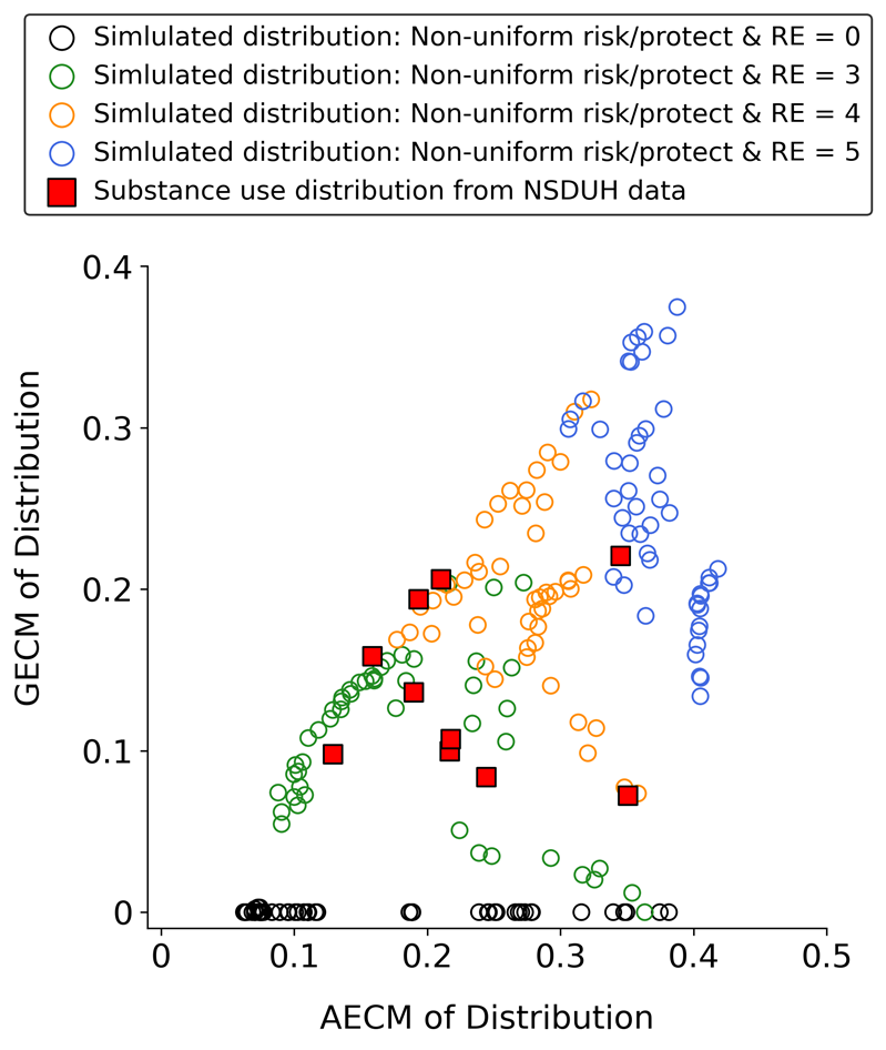
The results shown in Figure 10 correspond to the testing of the non-uniform distributions displayed in Stage 1 of Figure 4. Each circle in Figure 10 represents the GECM and AECM values of a simulated substance use frequency distribution generated by a specific combination of non-uniform distributions used to assign \(Pr(N \rightarrow U)\) and \(Pr(U \rightarrow N)_{t = 0}\). The results indicate that using non-uniform distributions does not impair the model’s ability to produce a range of U-shaped distributions with GECM and AECM values that are similar to those observed in the empirical NSDUH data. Furthermore, consistent with Figures 8 and 9, Figure 10 shows that setting the RE to zero (black circles) prevents the model from generating U-shaped distributions.
Analysis 3 results: Supplemental testing of alternative models (Appendix 3)
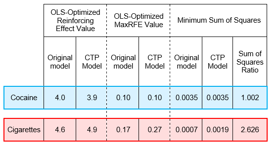
Supplemental Test 1 results demonstrated that the CTP model can generate plausible U-shaped distributions of substance use frequencies. Specifically, the CTP model fit for cocaine was comparable to the original model fit. However, for cigarettes, the CTP model produced a notably poorer fit. Supplemental Test 2.1 (i.e., assigning transition probabilities using distributions with means near 1 and 0) did not produce U-shaped distributions. However, Supplemental Test 2.2 (right-skewed distribution for assigning \(Pr(N \rightarrow U)\) values and U-shaped distribution for assigning \(Pr(U \rightarrow N)_{t = 0}\) values) successfully generated U-shaped substance use frequency distributions without relying on path dependence (see Appendix 3).
Discussion
Cross-sectional population distributions of past 30-day substance use frequencies are invariably “U-shaped” – regardless of the type of substance. The field of Substance Use Epidemiology does not have an explanatory model for this phenomenon. The present study sought to fill this gap by developing and testing a simple, intuitive, and theoretically-grounded computational model that provides a framework for explaining U-shaped distributions of population substance use frequencies. The model uses two core components to generate multiple longitudinal sequences of substance use: (1) two unique transition probabilities per object and (2) path dependence of decision-making. The results contribute to the scientific literature by demonstrating that these two simple components can reproduce the cross-sectional, U-shaped population distributions of consumption frequencies for multiple pharmacologically distinct classes of substances.
How do interactions between the three model inputs create U-shaped distributions?
To understand how this model generates U-shaped distributions, it is useful to examine the interactions among the three model inputs (RE, MinPFE, MaxRFE) for tobacco cigarettes, hallucinogens, and alcohol. Figure 6 illustrates that larger RE values (i.e., more path dependence) generated distributions with more data concentrated near the minimum and maximum possible use frequencies. For example, simulated tobacco and hallucinogen distributions had the highest RE values because, in the empirical (NSDUH) distributions of these two substances, daily consumers and once-in-the-past-month consumers comprised \(\geq\) 60% of all past-month consumers. However, the tobacco and hallucinogen NSDUH distributions were, in a certain sense, “opposites” of each other: Among past-month hallucinogen consumers, \(\sim\) 60% used once and \(\sim\) 1% used every day; among past-month tobacco consumers, \(\sim\) 6% used once and \(\sim\) 61% used every day. Simulating the extreme edge concentrations of these two substances required that both have high RE values. However, ensuring that they also had “opposite” oriented distributions required different ranges of risk and protective factor effect transition probabilities (Figure 7). Specifically, simulating the hallucinogen distribution required (1) narrow ranges of protective and risk probabilities to ensure that the majority of consumers had only used once in the past 30 days; (2) a high RE to overcome these narrow probability ranges and create a small number of daily consumers. On the other hand, the tobacco simulation required a wide range of protective and risk probabilities. Combining these wide ranges with a high RE allowed the tobacco distribution to be dominated by daily consumers. In contrast to tobacco and hallucinogens, the NSDUH alcohol data were less concentrated at the distribution edges (i.e., more heterogeneous use frequencies), with daily and single-day consumers accounting for only \(\sim\) 18% of all past 30-day alcohol consumers. Similar to tobacco, modeling the alcohol distribution required a wide range of protective and risk probabilities. However, unlike tobacco, alcohol required a much smaller RE (i.e., less path dependence) to generate its more gradually sloping distribution and smaller proportion of daily consumers.
Path dependence, Reinforcing Effect (RE) parameter, and U-shaped distributions
In this model, an object’s current decision is influenced by its prior decisions. Feedback loop concepts have been used in previous models of substance use (Epskamp et al. 2022; Mollick & Kober 2020; van den Ende et al. 2021). However, this study contributes to the science of substance use simulation by providing new evidence that path dependence can be a useful mechanism for accurately modeling population-level U-shaped distributions of substance use frequencies in the United States.
The interpretation of the RE parameter warrants further explanation. Increasing the RE introduces more path dependence, which, in turn, increases the chance that an object will become a daily user. A multitude of factors can cause a person to use a substance daily. One of these factors is the unique pharmacology of the substance. Different pharmacological classes of substances (e.g., nicotine, opioids, alcohol, cocaine) have different abuse liabilities and reinforcing values (Hursh & Roma 2013; Koffarnus 2023; Lynch & Carroll 2001). Therefore, the RE parameter could be conceptualized as corresponding to the unique pharmacological properties of a substance insofar as those properties dictate the probability of daily consumption. However, the RE cannot be interpreted entirely as pharmacology-based “addictiveness”, and it is inaccurate to claim that a substance has intrinsic reinforcing “properties”, or that one substance is “more addictive” than another (Higgins et al. 2004; Hughes et al. 1988). Despite varying pharmacological properties, every substance in the NSDUH data had daily consumers, which suggests that pharmacology is not the only factor that contributes to a substance’s reinforcing value. Factors such as routes of administration, dose, schedules and costs of reinforcement, alternative reinforcers, social networks, and many others play a strong (or stronger) role (Bickel et al. 1990, 2014; Hursh & Roma 2013; Koffarnus 2023; Roberts & Bennett 1993; Strickland & Acuff 2023; Watanabe 2011). Stated more simply, the factors that cause daily nicotine use may be very different from the factors that cause daily hallucinogen use or daily alcohol use. Consequently, the RE parameter may be more appropriately conceptualized as the combined result of the typical pharmacodynamic effects of a particular substance acting in conjunction with an unknown amalgam of environmental variables that modify such effects.
Path dependence and distributions of risk and protective factor transition probabilities
Results from Analyses 2a and 2b demonstrated that enabling path dependence allowed the model to generate U-shaped distributions with diverse GECM values, regardless of whether risk and protective factor transition probabilities were assigned using uniform or non-uniform starting distributions. This suggests that the model’s ability to generate U-shaped distributions relies less on the shape of the starting distributions of transition probabilities and more on combining path dependence with starting distributions that allow for a wide range of possible transition probabilities.
Alternative models
The CTP model results indicate that U-shaped distributions of substance use frequencies can also be simulated with a simpler model that requires only one input parameter for assigning transition probabilities to objects (rather than two parameters used in the original model). Notably, the CTP model fit was comparable to the original model fit for cocaine but not for cigarettes. This inconsistency in fit suggests that, while the CTP model provides a simpler alternative with fewer input requirements, its complementary structure may limit its ability to capture the full range of U-shaped distributions observed among different substances in the NSDUH data. Thus, for research requiring flexible representations of risk and protective factors, the original model may be more suitable, whereas the CTP model could be a viable alternative when an interdependent structure is conceptually appropriate.
Alternative model testing also indicated that path dependence is not essential for simulating U-shaped distributions. Supplemental Test 2.2 demonstrated that even without path dependence, a model can produce U-shaped distributions when protective factors are initialized with a U-shaped probability distribution (spanning from 0 to 1), and risk factors are initialized with a narrow, right-skewed distribution with a mean close to zero. However, this alternative approach requires a more complex set of starting distributions and additional parameter inputs. It also assumes protective factors in a population are bifurcated into two extremes: either highly protected or not protected at all. Although this scenario is possible, empirical evidence generally suggests a more gradual range of protective factors, with most individuals exhibiting a mix of strengths and vulnerabilities (Bry et al. 1982; Hawkins et al. 2004). Given this continuum, starting distributions such as uniform or Gaussian, rather than U-shaped, may better represent the broad range of protective factor levels observed in populations.
Integrating computational models into substance use epidemiology
This study expands on the current landscape of modeling in substance use epidemiology by re-evaluating basic assumptions and emphasizing the explanatory potential of simple computational models. While previous research has outlined the scientific and public health value of computational models (Auchincloss & Diez Roux 2008; Cerdà et al. 2021; Diez Roux 2011; Epstein 1999, 2008; Galea et al. 2009, 2010; Macal & North 2010; Silverman et al. 2021; Tracy et al. 2018) the model presented here highlights how simple, theory-driven mechanisms can explain complex substance use patterns. To better contextualize this approach, it is useful to consider other modeling techniques that are commonly employed.
Probability functions are commonly used in Substance Use Epidemiology and can be used to model U-shaped distributions. For example, setting alpha (a) and beta (b) to values between 0 and 1 in the beta probability density function \(f(x) = \frac{x(a - 1)(1 - x)(b - 1)}{B(a,b)}\) will yield U-shaped distributions. While these functions can describe and predict data patterns, they are not particularly helpful for exploring data-generating mechanisms and understanding how individual behaviors aggregate into unique population-level distributions.
Addressing this need, this study sought to determine whether U-shaped distributions of past 30-day substance use frequencies can be effectively modeled using two, simple, theoretically-justified assumptions: (1) each individual has a unique profile of risk and protective factors, and (2) prior decisions impact current decisions. This approach aligns with the KISS (Keep It Simple, Stupid) principle, which advocates for simple and intuitive models. There is a longstanding debate over the utility of simple models, and Edmonds offers two important points to consider. First, a modeling strategy like KISS is “…not something that can be proved right or wrong, merely more or less helpful in the experience of individual modellers” (Edmonds et al. 2019). Second, simplicity does not guarantee generalizability and complex models may be necessary “…when faced with obviously complex phenomena” (Edmonds 2018; Edmonds & Moss 2005) such as substance use. For example, complex sociodemographic disparities in risk and protective factors – such as income, geography, age, sex, and race/ethnicity (Galea et al. 2004) – influence substance use patterns and should be considered when interpreting a model’s assumptions and results. Although the simplicity of the model presented here offers a useful starting point, more complexity may be required to capture the nuances of substance use across diverse populations. Indeed, substance use researchers are increasingly using complex simulation models to explore a range of topics, such as socioeconomic and public health impacts of policies and treatments, social network influences, and drug market dynamics (Agar & Wilson 2002; Bobashev et al. 2020; Boyd et al. 2022; Cerdà et al. 2021; Combs et al. 2019; Hammond et al. 2020; Keane et al. 2018; Keyes et al. 2019; Ritter et al. 2016; van den Ende et al. 2021).
Limitations
This study has several limitations. First, the NSDUH sampling frame excludes homeless individuals, a group at high risk for substance use, which may lead to underestimates of heavier use patterns. Additionally, NSDUH data are based on self-report which is prone to measurement errors (e.g., poor recall, social stigma). Finally, data on prescription opioids, methamphetamine, hallucinogens, inhalants, and tranquilizers were only available from 2015 to 2019.
This study also excluded individuals who reported zero days of substance use in the past 30 days. This approach aligns with standard epidemiological definitions of "current use" and avoids interpretation problems associated with zero-inflation. However, it overlooks important subgroups such as "temporary abstainers," who have not used the substance within the last 30 days but have nonetheless used it at some point in the past (e.g., used within the past 365 days). Although this group is beyond the scope of the current study, their exclusion raises important questions about whether the individual-level longitudinal data produced by the model will accurately represent the cross-sectional diversity of use patterns over a wider timescale. For example, excluding those who reported zero days of substance use in the past 30 days may affect whether a cross-sectional analysis of the past 365 time steps of longitudinal trajectory patterns created by the model accurately represents the cross-sectional distribution of past-year use frequencies observed in the NSDUH data.
Another key limitation to emphasize is that the primary model presented in this study is not the only model capable of generating U-shaped distributions of simulated substance use frequencies. Supplemental analyses revealed that variations of the model – with both simpler and more complex design and parameter assumptions – can also produce similar U-shaped distributions. Conclusions about the primary model should be understood within this context.
Finally, this model does not explicitly account for social dynamics and interactions, which play a significant role in substance use. The model assumes that social influences are indirectly captured in the unique state transition probabilities of each object. Future studies could incorporate social components (e.g., peer pressure, social norms, etc.) to generate and test hypotheses about the role of social influences in substance use.
Future directions
This study demonstrated that population-level cross-sectional slices from the model’s individual-level longitudinal output closely resemble empirical cross-sectional data. However, the longitudinal data produced by the model could be used for other scientific purposes (Li & O’Donoghue 2012). To further validate the model, the next step is to assess whether its longitudinal data match empirical longitudinal substance use data. Establishing that a single model can reproduce distributions of empirical cross-sectional and longitudinal data would help “…reduce the risk of getting the right results for the wrong reasons” (Edmonds et al. 2019) and increase confidence in the model’s generalizability.
If the model’s longitudinal data accurately represents real-world substance use trajectories, it could be used to generate valuable insights into the strengths and limitations of common statistical methods in substance use research. For instance, longitudinal mixture models often yield a “Cats Cradle” pattern of results in highly disparate contexts, raising concerns that this pattern may be an artifact of data complexity rather than a true representation of substance use trajectories (Sher et al. 2011). The flexibility of the present model could enable systematic testing of this hypothesis.
Moreover, the model’s longitudinal data could also be used to develop testable hypotheses about the utility of alternative measures of substance use. For example, common measures, such as frequency of use (e.g., proportion of days used in the past 30 days), overlook the sequence of use. However, complexity measures (e.g., Lempel Ziv, Approximate Entropy, Permutation Entropy) could be used to detect differences in the sequence of substance use patterns. Such measures may have clinical utility if they allow us to discriminate future outcomes among seemingly homogenous groups of substance consumers.
Conclusion
This study advances Substance Use Epidemiology by introducing a computational model capable of replicating U-shaped distributions of substance use frequencies observed across diverse psychoactive substances. By incorporating individual-level risk and protective profiles alongside path dependence in decision-making, the model provides a framework for understanding how complex population patterns can emerge from simple, theory-driven assumptions. Future work could explore the model’s applications to both cross-sectional and longitudinal data, to better understand mechanisms driving substance use patterns and enhance the explanatory power of epidemiological models.
Appendix 1: Model Stability
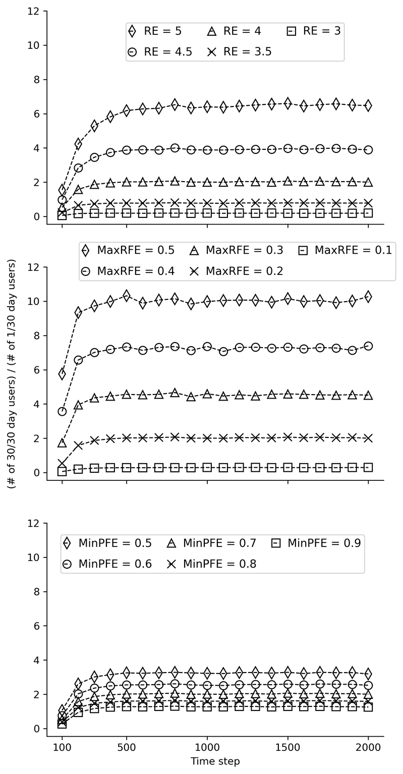
Results from model stability testing are provided in Figures 11, 12, and 13 below. The three figures present results from the same stability tests using different starting seeds. These tests aimed to determine the number of time steps required to stabilize the ratio of past 30-day daily users and once-per-month users. The three subgraphs (from left to right) within each figure correspond to tests of different values for each of the three modifiable parameters: Reinforcing Effect, Maximum Risk Factors Effect (MaxRFE), and Minimum Protective Factors Effect (MinPFE). In each subgraph, the values of one parameter are varied while the values of the other two are held constant. The outcome on the Y-axis was the ratio of the number of objects that had used on 30 of the past 30 time steps divided by the number of objects that had used on 1 of the past 30 time steps at each 100-step interval. For example, at the 100th time step, the number of steps that each object used during steps 70 to 100 was calculated (i.e., the last “30 days”). As is evident from the figures, the model is generally stable by the 1000th time step. Based on these results, 2000 time steps was chosen to increase confidence in the robustness of the results.


Appendix 2: Estimating Optimal Model Parameters
A least-squares approach was used for each substance to identify the best fit between each of the proportions in a simulated distribution of past 30-day use and the empirical distribution from the National Survey on Drug Use and Health (NSDUH). The optimization process used an iterative grid search that evaluated a set of parameter values to find the combination that yields the best result. The grid search was carried out over the Cartesian product of parameter values. Specifically, the search included MaxRFE and MinPFE values, which ranged from 0 to 1 in increments of 0.01, and Reinforcing Effect values, which ranged in increments of 0.1. If an optimal result for a parameter was found at the edge of the initial set of values, the search range was expanded to include more values in that direction. This allowed the search to continue beyond the initial range until an optimal value was identified. Multiple initial seeds were used during the estimation process to avoid the risk of converging on local minima. The results from this procedure correspond to the results presented in Figure 5 and Table 3 in the primary manuscript.
Appendix 3: Alternative Model Supplemental Tests
Supplemental test 1: Complementary Transition Probabilities (CTP) model
The CTP Model simplifies the original model by setting the protective factor transition probability \(P (U \rightarrow N)\) as the probability complement of the risk factor transition probability \(P (N \rightarrow U)\) (i.e., \(P (U \rightarrow N) = 1 - P (N \rightarrow U)\)). This approach reduces the number of input parameters required from the modeler. Overall, testing of the CTP Model indicated that it was capable of producing U-shaped distributions of substance use frequencies. However, to further explore its effectiveness, additional tests were conducted to compare the model’s ability to fit to the empirical (NSDUH) data for cocaine and cigarettes to that of the original model.
To evaluate the performance of the CTP Model, OLS optimization was used to determine the best-fit parameter values for cocaine and cigarettes (same process as described in Appendix 2). Specifically, an iterative grid search through the Cartesian product of Reinforcing Effect and MaxRFE parameter values was used to identify the minimum sum of squares fit to the empirical NSDUH data on past 30-day use frequencies. The optimized results were then compared to those obtained from the original model.
Supplemental Test 2: Models with U-shaped initialization distributions but no path dependence
Supplemental Test 2.1
Table 4 and Table 6 summarize the effects of using low-mean (near 0) and high-mean (near 1) initialization distributions (either highly skewed or narrow uniform) on the Geometric Edge Concentration Measure (GECM) of simulated substance use frequencies in a model that does not allow for path dependence. The results indicate that across all tested means for both risk and protective factor distributions, whether highly skewed or uniform, the GECM values remained at zero. This finding suggests that, in the absence of path dependence, even extreme initialization distributions concentrated near the boundaries of 0 and 1 do not result in U-shaped distributions of simulated substance use frequencies.
| Mean of right-skewed Risk Factor Distribution | Mean of left-skewed Protective Factor Distribution | Reinforcing Effect | GECM of simulated substance use distribution |
|---|---|---|---|
| 0.1 | 0.9 | 0 | 0 |
| 0.05 | 0.95 | 0 | 0 |
| 0.02 | 0.98 | 0 | 0 |
| 0.01 | 0.99 | 0 | 0 |
| 0.001 | 0.999 | 0 | 0 |
| 0.0001 | 0.9999 | 0 | 0 |
| Mean of Uniform Risk Factor Distribution | Mean of Uniform Protective Factor Distribution | Reinforcing Effect | GECM of simulated substance use distribution |
|---|---|---|---|
| 0.1 | 0.9 | 0 | 0 |
| 0.05 | 0.95 | 0 | 0 |
| 0.02 | 0.98 | 0 | 0 |
| 0.01 | 0.99 | 0 | 0 |
| 0.001 | 0.999 | 0 | 0 |
| 0.0001 | 0.9999 | 0 | 0 |
Supplemental Test 2.2
Supplemental Test 2.2 also aimed to determine whether U-shaped distributions of simulated substance use frequencies could be generated without enabling path dependence by utilizing specific initial probability distributions. Two initialization distributions were tested in tandem: (1) The risk factor distribution used to assign the \(P (N \rightarrow U)\) values was a highly right-skewed probability distribution with a mean close to zero, and (2) the protective factor distribution used to assign the \(P (U \rightarrow N)\) values was a U-shaped probability distribution with upward tails near zero and one (see top panel of Figure 14). This model was tested with the reinforcing effect set to zero (i.e., no path dependence). The example results from these tests illustrated in the bottom panel of Figure 15, demonstrate that simulated U-shaped distributions of substance use frequencies can be achieved without path dependence when using more complex initialization distributions.
Supplemental data
Supplemental data are available here: https://www.jasss.org/28/2/5/Supplemental_data_Fig9.xlsx
References
AGAR, M. H., & Wilson, D. (2002). Drugmart: Heroin epidemics as complex adaptive systems. Complexity, 7(5), 44–52. [doi:10.1002/cplx.10040]
AUCHINCLOSS, A. H., & Diez Roux, A. V. (2008). A new tool for epidemiology: The usefulness of dynamic-agent models in understanding place effects on health. American Journal of Epidemiology, 168(1), 1–8. [doi:10.1093/aje/kwn118]
BICKEL, W. K., DeGrandpre, R. J., Higgins, S. T., & Hughes, J. R. (1990). Behavioral economics of drug self-administration. I. Functional equivalence of response requirement and drug dose. Life Sciences, 47(17), 1501–1510. [doi:10.1016/0024-3205(90)90178-t]
BICKEL, W. K., Johnson, M. W., Koffarnus, M. N., MacKillop, J., & Murphy, J. G. (2014). The behavioral economics of substance use disorders: Reinforcement pathologies and their repair. Annual Review of Clinical Psychology, 10, 641–677. [doi:10.1146/annurev-clinpsy-032813-153724]
BOBASHEV, G., Mars, S., Murphy, N., Dreisbach, C., Zule, W., & Ciccarone, D. (2020). Heroin type, injecting behavior, and HIV transmission. A simulation model of HIV incidence and prevalence. PLoS One, 14(12), e0215042. [doi:10.1371/journal.pone.0215042]
BOYD, J., Wilson, R., Elsenbroich, C., Heppenstall, A., & Meier, P. (2022). Agent-Based modelling of health inequalities following the complexity turn in public health: A systematic review. International Journal of Environmental Research and Public Health, 19(24), 24. [doi:10.3390/ijerph192416807]
BRY, B. H., McKeon, P., & Pandina, R. J. (1982). Extent of drug use as a function of number of risk factors. Journal of Abnormal Psychology, 91(4), 273–279. [doi:10.1037//0021-843x.91.4.273]
BURGETTE, L. F., Cabreros, I., Han, B., & Paddock, S. M. (2021). Appropriate analyses of bimodal substance use frequency outcomes: A mixture model approach. The American Journal of Drug and Alcohol Abuse, 47(5), 559–568. [doi:10.1080/00952990.2021.1946070]
CATANIA, A. C. (2010). The operant behaviorism of B. F. Skinner. Behavioral and Brain Sciences, 7(4), 473–475. [doi:10.1017/s0140525x00026728]
CENTER for Behavioral Health Statistics and Quality. (2020a). National survey on drug use and health (2002—2019) codebook. Substance Abuse and Mental Health Services Administration.
CENTER for Behavioral Health Statistics and Quality. (2020b). National survey on drug use and health (2019): Methodological summary and definitions. Substance Abuse and Mental Health Services Administration.
CERDÀ, M., Jalali, M. S., Hamilton, A. D., DiGennaro, C., Hyder, A., Santaella-Tenorio, J., Kaur, N., Wang, C., & Keyes, K. M. (2021). A systematic review of simulation models to track and address the opioid crisis. Epidemiologic Reviews, 43(1), 147–165.
COMBS, T. B., McKay, V. R., Ornstein, J., Mahoney, M., Cork, K., Brosi, D., Kasman, M., Heuberger, B., Hammond, R. A., & Luke, D. (2019). Modelling the impact of menthol sales restrictions and retailer density reduction policies: Insights from tobacco town Minnesota. Tobacco Control, 29(5), 502–509. [doi:10.1136/tobaccocontrol-2019-054986]
DAVID, P. A. (2007). Path dependence: A foundational concept for historical social science. Cliometrica, 1(2), 91–114. [doi:10.1007/s11698-006-0005-x]
DIEZ Roux, A. V. (2011). Complex systems thinking and current impasses in health disparities research. American Journal of Public Health, 101(9), 1627–1634. [doi:10.2105/ajph.2011.300149]
EDMONDS, B. (2018). A bad assumption: A simpler model is more general. Available at: https://rofasss.org/2018/08/28/be-2/
EDMONDS, B., Le Page, C., Bithell, M., Chattoe-Brown, E., Grimm, V., Meyer, R., Montañola-Sales, C., Ormerod, P., Root, H., & Squazzoni, F. (2019). Different modelling purposes. Journal of Artificial Societies and Social Simulation, 22(3), 6. [doi:10.18564/jasss.3993]
EDMONDS, B., & Moss, S. (2005). From KISS to KIDS - an ’anti-simplistic’ modelling approach. In P. Davidsson, B. Logan, & K. Takadama (Eds.), Multi-Agent and Multi-Agent-Based Simulation (pp. 130–144). Berlin Heidelberg: Springer. [doi:10.1007/978-3-540-32243-6_11]
EPSKAMP, S., van der Maas, H. L. J., Peterson, R. E., van Loo, H. M., Aggen, S. H., & Kendler, K. S. (2022). Intermediate stable states in substance use. Addictive Behaviors, 129, 107252. [doi:10.1016/j.addbeh.2022.107252]
EPSTEIN, J. M. (1999). Agent-based computational models and generative social science. Complexity, 4(5), 41–60. [doi:10.1002/(sici)1099-0526(199905/06)4:5<41::aid-cplx9>3.0.co;2-f]
EPSTEIN, J. M. (2008). Why model? Journal of Artificial Societies and Social Simulation, 11(12), 4.
GALEA, S., Hall, C., & Kaplan, G. A. (2009). Social epidemiology and complex system dynamic modelling as applied to health behaviour and drug use research. International Journal of Drug Policy, 20(3), 209–216. [doi:10.1016/j.drugpo.2008.08.005]
GALEA, S., Nandi, A., & Vlahov, D. (2004). The social epidemiology of substance use. Epidemiologic Reviews, 26(1), 36–52. [doi:10.1093/epirev/mxh007]
GALEA, S., Riddle, M., & Kaplan, G. A. (2010). Causal thinking and complex system approaches in epidemiology. International Journal of Epidemiology, 39(1), 97–106. [doi:10.1093/ije/dyp296]
GRIMM, V., Berger, U., Bastiansen, F., Eliassen, S., Ginot, V., Giske, J., Goss-Custard, J., Grand, T., Heinz, S. K., Huse, G., Huth, A., Jepsen, J. U., JNørgensen, C., Mooij, W. M., Müller, B., Pe’er, G., Piou, C., Railsback, S. F., Robbins, A. M., … DeAngelis, D. L. (2006). A standard protocol for describing individual-based and agent-based models. Ecological Modelling, 198(1), 115–126. [doi:10.1016/j.ecolmodel.2006.04.023]
GRIMM, V., Railsback, S. F., Vincenot, C. E., Berger, U., Gallagher, C., DeAngelis, D. L., Edmonds, B., Ge, J., Giske, J., Groeneveld, J., Johnston, A. S. A., Milles, A., Nabe-Nielsen, J., Polhill, J. G., Radchuk, V., Rohwäder, M. S., Stillman, R. A., Thiele, J. C., & Ayllón, D. (2020). The ODD protocol for describing agent-based and other simulation models: A second update to improve clarity, replication, and structural realism. Journal of Artificial Societies and Social Simulation, 23(2), 7. [doi:10.18564/jasss.4259]
HAMMOND, R. A. (2015). Considerations and best practices in agent-Based modeling to inform policy. https://www.ncbi.nlm.nih.gov/books/NBK305917/
HAMMOND, R. A., Combs, T. B., Mack-Crane, A., Kasman, M., Sorg, A., Snider, D., & Luke, D. A. (2020). Development of a computational modeling laboratory for examining tobacco control policies: Tobacco Town. Health Place, 61, 102256. [doi:10.1016/j.healthplace.2019.102256]
HAWKINS, J. D., Horn, M. L. V., & Arthur, M. W. (2004). Community variation in risk and protective factors and substance use outcomes. Prevention Science, 5(4), 213–220. [doi:10.1023/b:prev.0000045355.53137.45]
HIGGINS, S. T., Heil, S. H., & Lussier, J. P. (2004). Clinical implications of reinforcement as a determinant of substance use disorders. Annual Review of Psychology, 55, 431–461. [doi:10.1146/annurev.psych.55.090902.142033]
HUGHES, J. R., Higgins, S. T., & Bickel, W. K. (1988). Behavioral "properties" of drugs. Psychopharmacology, 96(4), 557. [doi:10.1007/bf02180040]
HURSH, S. R., & Roma, P. G. (2013). Behavioral economics and empirical public policy. Journal of the Experimental Analysis of Behavior, 99(1), 98–124. [doi:10.1002/jeab.7]
KEANE, C., Egan, J. E., & Hawk, M. (2018). Effects of naloxone distribution to likely bystanders: Results of an agent-based model. International Journal of Drug Policy, 55, 61–69. [doi:10.1016/j.drugpo.2018.02.008]
KEYES, K. M., Shev, A., Tracy, M., & Cerda, M. (2019). Assessing the impact of alcohol taxation on rates of violent victimization in a large urban area: An agent-based modeling approach. Addiction, 114(2), 236–247. [doi:10.1111/add.14470]
KLESGES, R. C., Debon, M., & Ray, J. W. (1995). Are self-reports of smoking rate biased? Evidence from the second national health and nutrition examination survey. Journal of Clinical Epidemiology, 48(10), 1225–1233. [doi:10.1016/0895-4356(95)00020-5]
KLEVMARKEN, A. (2022). A brief survey of behavioral modeling in micro simulation models. International Journal of Microsimulation, 15(1).
KOFFARNUS, M. N. (2023). Recommendations for the use of behavioral economic demand as an abuse liability assessment for drug scheduling. Policy Insights from the Behavioral and Brain Sciences, 10(1), 113–120. [doi:10.1177/23727322221150197]
LI, J., & O’Donoghue, C. (2012). A survey of dynamic microsimulation models: Uses, model structure andmethodology. International Journal of Microsimulation, 6(2), 3–55. [doi:10.34196/ijm.00082]
LI, J., & O’Donoghue, C. (2014). Evaluating binary alignment methods in microsimulation models. Journal of Artificial Societies and Social Simulation, 17(1), 15. [doi:10.18564/jasss.2334]
LYNCH, W. J., & Carroll, M. E. (2001). Regulation of drug intake. Experimental and Clinical Psychopharmacology, 9(2), 131–143. [doi:10.1037//1064-1297.9.2.131]
MACAL, C. M., & North, M. J. (2010). Tutorial on agent-based modelling and simulation. Journal of Simulation, 4(3), 151–162. [doi:10.1057/jos.2010.3]
MOLLICK, J. A., & Kober, H. (2020). Computational models of drug use and addiction: A review. Journal of Abnormal Psychology, 129(6), 544–555. [doi:10.1037/abn0000503]
PANLILIO, L. V., & Goldberg, S. R. (2007). Self-administration of drugs in animals and humans as a model and an investigative tool. Addiction, 102(12), 1863–1870. [doi:10.1111/j.1360-0443.2007.02011.x]
PORGO, T. V., Norris, S. L., Salanti, G., Johnson, L. F., Simpson, J. A., Low, N., Egger, M., & Althaus, C. L. (2019). The use of mathematical modeling studies for evidence synthesis and guideline development: A glossary. Research Synthesis Methods, 10(1), 125–133. [doi:10.1002/jrsm.1333]
RHODES, T., Lilly, R., Fernández, C., Giorgino, E., Kemmesis, U. E., Ossebaard, H. C., Lalam, N., Faasen, I., & Spannow, K. E. (2003). Risk factors associated with drug use: The importance of ’risk environment’. Drugs: Education, Prevention and Policy, 10(4), 303–329. [doi:10.1080/0968763031000077733]
RITTER, A., Shukla, N., Shanahan, M., van Hoang, P., Cao, V. L., Perez, P., & Farrell, M. (2016). Building a microsimulation model of heroin use careers in Australia. International Journal of Microsimulation, 9(3), 140–176. [doi:10.34196/ijm.00146]
ROBERTS, D. C. S., & Bennett, S. A. L. (1993). Heroin self-administration in rats under a progressive ratio schedule of reinforcement. Psychopharmacology, 111(2), 215–218. [doi:10.1007/bf02245526]
SHER, K. J., Jackson, K. M., & Steinley, D. (2011). Alcohol use trajectories and the ubiquitous cat’s cradle: Cause for concern? Journal of Abnormal Psychology, 120, 322–335. [doi:10.1037/a0021813]
SILVERMAN, E., Gostoli, U., Picascia, S., Almagor, J., McCann, M., Shaw, R., & Angione, C. (2021). Situating agent-based modelling in population health research. Emerging Themes in Epidemiology, 18(1), 10. [doi:10.1186/s12982-021-00102-7]
SLOBODA, Z., Glantz, M. D., & Tarter, R. E. (2012). Revisiting the concepts of risk and protective factors for understanding the etiology and development of substance use and substance use disorders: Implications for prevention. Substance Use & Misuse, 47(8–9), 944–962. [doi:10.3109/10826084.2012.663280]
SPIELAUER, M. (2011). What is social science microsimulation? Social Science Computer Review, 29(1), 9–20. [doi:10.1177/0894439310370085]
STONE, A. L., Becker, L. G., Huber, A. M., & Catalano, R. F. (2012). Review of risk and protective factors of substance use and problem use in emerging adulthood. Addictive Behaviors, 37(7), 747–775. [doi:10.1016/j.addbeh.2012.02.014]
STRICKLAND, J. C., & Acuff, S. F. (2023). Role of social context in addiction etiology and recovery. Pharmacology Biochemistry and Behavior, 229, 173603. [doi:10.1016/j.pbb.2023.173603]
TARANTOLA, A. (2023). Inverse problem. https://mathworld.wolfram.com/InverseProblem.html
TRACY, M., Cerda, M., & Keyes, K. M. (2018). Agent-based modeling in public health: Current applications and future directions. Annual Review of Public Health, 39, 77–94. [doi:10.1146/annurev-publhealth-040617-014317]
TURNER, J. R., & Baker, R. M. (2019). Complexity theory: An overview with potential applications for the social sciences. Systems, 7(1), 4.
VAN den Ende, M. W. J., Epskamp, S., Lees, M. H., VAN der Maas, H. L. J., Wiers, R. W., & Sloot, P. M. A. (2021). A review of mathematical modeling of addiction regarding both (neuro-) psychological processes and the social contagion perspectives. Addictive Behaviors, 127, 107201. [doi:10.1016/j.addbeh.2021.107201]
VAN Imhoff, E., & Post, W. (1998). Microsimulation methods for population projection. Population: An English Selection, 10(1), 97–138. [doi:10.3917/popu.p1998.10n1.0136]
VOLLMER, T. R., & Hackenberg, T. D. (2001). Reinforcement contingencies and social reinforcement: Some reciprocal relations between basic and applied research. Journal of Applied Behavior Analysis, 34(2), 241–253. [doi:10.1901/jaba.2001.34-241]
WAGNER, B., Riggs, P., & Mikulich-Gilbertson, S. (2015). The importance of distribution-choice in modeling substance use data: A comparison of negative binomial, beta binomial, and zero-inflated distributions. The American Journal of Drug and Alcohol Abuse, 41(6), 489–497. [doi:10.3109/00952990.2015.1056447]
WANG, H., & Heitjan, D. F. (2008). Modeling heaping in self-reported cigarette counts. Statistics in Medicine, 27(19), 3789–3804. [doi:10.1002/sim.3281]
WATANABE, S. (2011). Drug-social interactions in the reinforcing property of methamphetamine in mice. Behavioural Pharmacology, 22(3), 203. [doi:10.1097/fbp.0b013e328345c815]
WILSON, R. C., & Collins, A. G. E. (2019). Ten simple rules for the computational modeling of behavioral data. eLife, 8, e49547. [doi:10.7554/elife.49547]