Finance and Market Concentration Using Agent-Based Modeling: Evidence from South Korea

,
,
,
and
aSamsung Global Research, South Korea; bDepartment of Industrial Engineering, Korea Advanced Institute of Science and Technology (KAIST), South Korea; c Department of Data Science, Korea Advanced Institute of Science and Technology (KAIST), South Korea; d Department of Convergence Business, Korea University, South Korea.
Journal of Artificial
Societies and Social Simulation 28 (3) 5
<https://www.jasss.org/28/3/5.html>
DOI: 10.18564/jasss.5710
Received: 04-Mar-2024 Accepted: 12-May-2025 Published: 30-Jun-2025
Abstract
This study investigates the role of finance in shaping the global trend of increasing market concentration. Using agent-based modeling (ABM), we conduct qualitative and quantitative analyses to examine the impact of financial policies on market concentration. Additionally, we analyze their simultaneous effects on economic growth and labor income share as key macroeconomic indicators. Building upon the Keynes meets Schumpeter (K+S) model, we conduct policy experiments using a model validated against the historical trends in South Korea. For the policy variables,we apply the debt-to-sales ratio (DSR) limit and interest rate as levers to regulate the quantity and cost of finance, respectively. The simulation results show that lowering interest rates alleviates market concentration while DSR regulation exhibits nonlinear effects on it. As the DSR limit increases, market concentration initially decreases but rises again beyond a certain threshold. To investgiate the rationale behind this phenomenon, we examine how finance affects individual firms at a micro level through firm-level analysis. Our findings underscore the value of ABM in addressing this complex issue from both the micro and macro perspectives. Moreover, they highlight that the impact on market concentration varies based on the nature of financial policies, and suggest that coordinating DSR regulatory policies with monetary policies such as interest rates can help policymakers manage market concentration.Introduction
In recent years, market concentration – the degree to which a small group of firms dominates a market – has increased in many countries including the United States, the Netherlands, and China (Akcigit & Ates 2021a; Cerdeiro & Ruane 2022; Freeman et al. 2021). However, an excessive market concentration often creates market inefficiency. For example, as the market power of large firms increases, productivity competition may stagnate, consumer prices may increase, and barriers to entry for new firms may increase. Moreover, market concentration is closely linked to traditionally important macroeconomic factors such as economic growth and labor income share. Thus, market concentration has emerged as a key analytical subject for policymakers and researchers.
Amid previous studies examining the factors affecting market concentration (Davis & Haltiwanger 2014; Gordon 2016; Karahan et al. 2019), the role of financing has gained attention. The questions posed by researchers are clear: Does finance exacerbate (or alleviate) polarization among firms? What side effects does finance have on economic growth and labor income share? The literature contains varying views on these questions, depending on the financial policies, assumptions, or models they employ.
However, previous studies overlooked the interactions among the agents. Indeed, a firm’s growth, which is a micro factor of market concentration, is influenced by the behaviors of other agents in the market. For instance, innovation results, as key drivers of growth, diffuse from one firm to competitors because firms imitate each other’s technologies. Additionally, a firm’s growth is heavily influenced by the level of technology of its suppliers and the extent of its transactions with them. In addition, banks selectively provide limited financing to firms based on their preferences. Finally, the wage that the household receives is affected by the average level of labor productivity in the economy; therefore, one firm’s increase in productivity may indirectly affect other firms’ burden of hiring labor. Previous methods, such as dynamic stochastic general equilibrium (DSGE) or traditional statistical models, fail to account for the influence of complicated interactions on aggregated variables.
In this regard, we employ ABM to investigate the impact of finance on market concentration. This approach aims to capture the complex interactions among the agents mentioned above, a factor that previous works do not consider. Specifically, we extend the Keynes-meets-Schumpeter (K+S) model for macroeconomic modeling (Dosi et al. 2010, 2013), which models technological diffusion, imperfect competition among firms, and unequal banking priorities toward these firms. We further improve the model in three ways. First, to analyze the changes in labor income share over finance, we replace the Leontief production function with the Cobb-Douglas function, allowing for substitution between labor and capital. Second, we incorporate the diminishing marginal improvement of technology into our model to offer a more accurate explanation of the reality, in which the level of investment required for equivalent technological development increases as technology advances. Third, we validate the model using historical data from South Korea from 1990 to 2020. Our model fits the historical trend, whereas previous work (Guerini & Moneta 2017) conducted structural validation with the K+S model.
Using the validated model, we conduct policy experiments to analyze how financing affects market concentration, economic growth, and labor income share. We employ two major financial policies as proxies for finance: the debt-to-sales ratio(DSR) and the interest rate, which represent control over the quantity and cost of financing, respectively. The experiments aim to answer the following research questions.
RQ 1. Does finance intensify or alleviate market concentration? This is the core question of this study. The crucial factor is whether finance strengthens the supremacy of a handful of major firms or promotes the growth of small and medium-sized enterprises, thus mitigating market polarization. We aimed to determine whether our ABM approach produces results consistent with those of previous studies or offers a different perspective.
RQ 1-1. How is financing allocated among different firms? This question is posed to analyze the rationale behind the aggregated result in RQ 1 at the micro level. Specifically, we examine whether financing is provided to every firm at its maximum level. We investigate how these findings contribute to macroeconomic variables.
RQ 2. (Side effects) Does finance facilitate economic growth and lower the labor income share? While focusing primarily on market concentration, this study examines the side effects of financial policies on economic growth and labor income share—macroeconomic variables closely related to market concentration. We aim to identify any trade-offs between these variables and market concentration and whether the relationships among these variables align with those of previous studies.
The remainder of this paper is organized as follows. The Literature Review section provides a review of prior studies that examine the effect of finance on market concentration, economic growth, and labor income share. This section also compares our ABM approach with methodologies previously employed for this topic, identifying the gaps that our approach can address. The Model Description section offers a comprehensive explanation of our model and elucidates the simulation steps that form its foundation. The Output Validation Section provides the quantitative and qualitative analysis on the validation results. With the validated model, the Policy Experiment section provides the results of the policy experiments and thoroughly analyze the effect of financing on market concentration and side effects. Finally, the Conclusion section summarizes the key findings and contributions of this study and discusses the limitations and potential areas for further research.
Literature Review
This section reviews the arguments and methodologies used in previous studies related to our research questions. In the first subsection, we review the literature on the various effects of financing on market concentration, which is our primary focus. Specifically, we explore how previous studies addressed this topic and establish a basis for comparison to analyze how the results in our study differ. The second subsection delves into prior research on the financial impact on economic growth and labor income share. We also elaborate on how economic growth and the labor income share are connected to market concentration in earlier studies. This provides the rationale for our decision to specifically analyze economic growth and labor income share to assess the side effects of finance on market concentration. In the final subsection, we compare various methodologies used to investigate our research questions. This study is not the first to raise these questions, but it is the first to utilize the agent-based model to answer them.
The impact of finance on market concentration
The impact of finance on market concentration has been studied separately based on two types of policies: those that regulate the cost of financing and those that adjust the quantity of financing. For both types of policies, there are opposing perspectives: one perspective states that financing alleviates market concentration, whereas the other states that it intensifies market concentration.
In terms of the cost of finance, there are two contrasting perspectives on how changes in interest rates impact market concentration. From an alleviation perspective, numerous researchers argue that lowering interest rates reduces market concentration by benefiting small firms, whereas increasing interest rates exacerbate market concentration. Cooley & Quadrini (2006), Carlstrom & Fuerst (1997), Gertler & Bernanke (1989) contend that low interest rates alleviate the burden of debt and improve the net worth of small firms. Thus, small firms are eligible to borrow larger amounts from banks at reduced costs. In addition, Cloyne et al. (2018) claim that the collateral value increases when interest rates decrease, allowing small firms to secure larger loans. All these effects are more pronounced in small firms than in large firms because the assets of small firms predominantly consist of debt. By contrast, large firms with sufficient internal funding capabilities are less reliant on debt financing. Moreover, Banerjee & Hofmann (2018), Caballero et al. (2008), Adalet et al. (2018) argue that reduced financial pressure resulting from lowered interest rates prolongs the survival of zombie firms that struggle to cover their debt with their profits. They argue that in this manner, the restructuring or exit of zombie firms may be deferred, contributing to an inefficiently low market concentration. In the same vein, some argue that rising interest rates make it difficult for small firms to survive, leading to increased market concentration. When interest rates increase, small firms may face challenges in transitioning from bank lending to alternative sources of funding to ensure liquidity because capital markets are imperfect (Gertler & Bernanke 1989; Kiyotaki & Moore 1997). Lastly, according to Bernanke et al. (1996), increased interest rates trigger the ‘’flight-to-quality’’ dynamics, wherein investors prefer risk-free projects offered by large firms.
Conversely, from an intensifying perspective, several studies suggest that lower interest rates give large firms stronger incentives to invest and grow faster, thereby exacerbating market concentration. Ottonello & Winberry (2020) contend that the difference is in the marginal cost of investment across firms. According to these studies, when investment scales up, large firms that already have sufficient financing or can rely on internal financing, experience a much smaller increase in marginal costs. Furthermore, Liu et al. (2022) and Kroen et al. (2021) contend that as interest rates decline, large firms intentionally pursue aggressive investment to widen the productivity gap with small firms and fortify entry barriers in the market. This is attributed to the increased future value of maintaining a market-leader position and generating significant profits as interest rates decrease.
In terms of policies that regulate the quantity of financing, previous studies can be divided into two opposing perspectives: financing either alleviates or intensifies market concentration. From an alleviating perspective, Greenwood & Jovanovic (1990), Beck et al. (2005) emphasize that small firms experience significant growth under financial development, which enhances their accessibility to finance. They argue that financing provides increased investment opportunities for small firms previously constrained by insufficient capital investment. Furthermore, Krishnan et al. (2014), Chen & Lee (2023) assert that productivity improvements in small firms are more responsive to financial supply than those in large firms. They find that banking deregulation, which increases financial accessibility for firms, results in a more significant productivity increase for small firms than for large firms.
In contrast, from an intensifying perspective, specific financial deregulation provides larger firms with enhanced financial access. Liu & Chen (2023) asserts that information asymmetry between borrowers (firms) and the lenders (banks) decreases as firm size increases. When bank branching is deregulated, small firms undergo adverse selection from bank branches, whereas large firms, whose information is relatively more disclosed to numerous bank branches, experience greater opportunities to secure loans. In this regard, the ‘’rich-get-richer’’ phenomenon can be observed with loosening financial regulations. Amid these diverse and contrasting perspectives on how finance impacts market concentration, we explore how the results differ using ABM compared to the existing findings.
Macroeconomic factors linked to market concentration: Growth and labor share
Market concentration is significant in its own right, but is also closely correlated with macroeconomic variables such as economic growth and the labor income share, which represent growth and distribution. Consequently, the relationship among these three factors are often studied together. The literature provides theoretical evidence that market concentration and labor income share generally have a negative correlation (Akcigit & Ates 2021a). However, views on the relationship between market concentration and economic growth vary. Some argue that strong market concentration impedes economic growth because it reduces firms’ profits (Singh 2004) or monopoly rents (Schumpeter 1943). Conversely, some studies argue that a high market concentration, which intensifies competition among firms, leads to an increase in average productivity (Arrow 2009; Schumpeter 1943) and encourages new firms to introduce innovative technologies into the market (Van Stel et al. 2019), thereby promoting economic growth.
In the context of our research focusing on the impact of finance, it is meaningful to examine how economic growth and the labor income share are affected, while analyzing how market concentration changes. We revisit the dynamics of the individual impact of finance on market concentration, economic growth, and labor income share, and the relationships between market concentration, economic growth, and labor income share within a single ABM framework. Specifically, we explore how changes in financial variables affect these three factors individually, and assess whether their existing relationships are maintained. ABM holds particular significance in this analysis because it derives macroeconomic variables from the bottom-up, modeling the behaviors of agents independently, rather than relying on a statistical model.
How have previous studies addressed the impact of finance on economic growth and labor income share? Finance has traditionally been acknowledged for its role in fostering economic growth (Beck et al. 2000; Beck & Levine 2004; Levine 2005). However, opposing viewpoints consistently suggest that excessive financing may impede economic growth (Arcand et al. 2015). In particular, following the 2008 financial crisis, certain studies indicated a nonlinear relationship between economic growth and finance (Arcand et al. 2015; Cecchetti & Kharroubi 2012).
Prior studies sought to identify the causal relationship between the recent decline in labor income share and financial. First, several studies focus on how financialization induces firms to prioritize the interests of shareholders, resulting in an increase in capital income share and a decrease in labor income share. As shareholders empower firms to generate returns from short-term profits, they often reduce employment, cut wages, and distribute higher dividends to shareholders. Numerous studies support this ‘’downsize–distribute principle,’’ (Blecker 2016; Cynamon & Fazzari 2015; Hein 2019; Palley 2015; Van Treeck 2015). Additionally, Wood (2016) contend that the increased household indebtedness resulting from an expansionary monetary policy may contribute to the declining labor income share. They argue that households with substantial debt in their desperation to secure future employment experience weakened their bargaining positions in wage negotiations.
Limitations in the methodologies of previous research
The gap in the existing research lies in the methodology. Analyses conducted using traditional statistical models, such as regression models, often successfully replicate the empirical evidence of high market concentration, slowed economic growth, and decreased labor income share. However, they can be prone to overfitting existing data, because they lack a robust micro-foundation in macroeconomics. In addition, in our context, they cannot account for the complicated mechanism behind the explicit correlations between finance and market concentration, such as the finance-induced disparity among firms through the productivity gap.
Studies conducted using a DSGE model cannot account for firm interactions arising from non-equilibrium states, a crucial aspect in analyzing market concentration. The fixed-point method of DSGE, designed to calculate a theoretically unique equilibrium, addresses neither the possibility of reaching equilibrium nor the path to reach it. However, in reality, various interactions among firms in non-equilibrium states influence which firms grow faster and which are phased out. Consequently, the economy can reach a different equilibrium of market concentration depending on the starting point and interaction among firms.
As an alternative, we utilized ABM, which not only provides a bottom-up explanation that accounts for agents’ behavior at the micro level, but also captures the intricate emergent patterns resulting from interactions among the firms. Within the ABM framework ABM, one can readily identify several examples of feedback loops in the context of market concentration. When a certain group of firms accumulates enough liquidity and generates substantial profits, they can access more loans, while other firms may miss out on borrowing opportunities due to limited credit in the economy. Conversely, once small firms experience reduced debt burden through financial support, they can catch up with larger firms over time. In terms of the productivity gap, technology diffusion can either accelerate or decelerate gap widening. Although it remains uncertain whether the loops within a single model would reinforce or balance each other, it is evident that these intricate interactions among the agents and initial states significantly influence which equilibrium or non-equilibrium the model reaches over time. In this regard, despite the shortcomings of ABM compared with DSGE, there are areas where ABM can contribute in the context of finance and market concentration, and it is worth analyzing those areas of potential contribution.
Model Description
To evaluate the impact of financing on market concentration, we introduce a macroeconomic agent-based model. Our model is based on the credit-augmented Keynes-meets-Schumpeter (K+S) framework proposed in Dosi et al. (2013). From a modeling perspective, we incorporate two major modifications compared with the K+S model. These modifications address the three factors governing firm growth – capital, labor, and technology. The traditional K+S model oversimplifies these factors, which can distort market concentration. Therefore, revising these assumptions to reflect reality better is essential for our research.
First, we replace the production function of the K+S model, originally a Leontief function, with a Cobb-Douglas (CD) function. This is essential to our research on the impact of financing on market concentration. Market concentration evolves based on the differences in growth rates among firms. The extent to which a firm grows depends on how it allocates its budget between employment and investment under a given financial policy. If all firms allocate their budgets in the same proportion between employment and investment because of the constraints of a Leontief function, any changes in financial policy would inevitably distort firm growth, and consequently, market concentration. However, by introducing the CD function, which allows for sustainability between labor and capital, we alleviate these limitations.
Second, we incorporate the assumption of diminishing marginal improvement in technology into our model. The K+S model relies on the constant marginal improvement of the technology assumption, where the cost of technological development and the speed of technological advancement remain constant, regardless of the current level of technology. However, several studies argue that large firms with a high current level of technology exhibit lower technological advancement efficiency because of the complexity and maturity of their existing technologies. Some studies (Audretsch & Acs 1991; Bloom et al. 2020; Kim 2018) suggest that compared to small firms, large firms are heavily reliant on their existing technologies, which makes it difficult for them to undergo creative destruction. Numerous studies and reports indicate that returns on R&D diminish in various industries, such as the pharmaceutical and semiconductor sectors (Aboagye et al. 2014; Graves & Langowitz 1993). In this regard, we extend the model from one where R&D success depends solely on the absolute amount of R&D expenditure to one where both the probability and speed of R&D success increase with R&D expenditure but decrease as the current technological level advances. This second modification is as crucial as the first in understanding market concentration, as each firm’s growth depends on how often and significantly its machine supplier’s R&D succeeds, along with its decisions on employment and investment. Moreover, by introducing this assumption, our new model, which incorporates a CD production function, achieves a better alignment with and validation against real-world trends.
Agents and their interactions in four markets
Our model comprises four types of agents. The first agent is capital-goods firms (referred to as K-firms), representing the R&D sector, and the model includes \(N_{F_K}\) heterogeneous K-firms. The second agent comprises consumption-goods firms (referred to as C-firms) representing the manufacturing sector, and the model includes \(N_{F_C}\) heterogeneous C-firms. The third agents are household agents responsible for labor and consumption in the model. The model has \(N_H\) household agents and we assume homogeneous labor and consumption preferences for all households. The fourth agent type is banks, which represent the financial sector. For simplicity, this model includes only one bank agent.
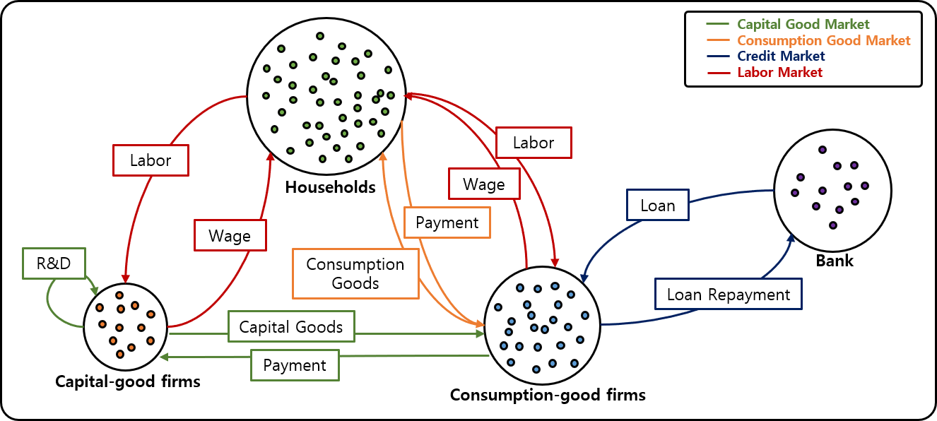
The main interactions between agents are shown in Figure 1. As these interactions are reinforced or mitigated over numerous time steps, heterogeneity among agents and complex emergent phenomena emerge randomly. First, in the capital goods market, as denoted by green, K-firms innovate or imitate machines from other firms to improve their productivity. These firms then produce and sell their machines to C-firms by advertising their products via brochures. Since the machines differ in performance and price, and not all brochures are identically delivered to all clients but are delivered mainly to historical clients, this capital goods market is an oligopoly market with information asymmetry. The machines that each C-goods firm buys determine its efficiency in producing its consumption good, and thereby, its price competitiveness. In the consumption goods market, denoted by orange, the C-firms produce homogeneous goods and sell them to households. Firms compete on price, as in Bertrand competition, but their market shares are inversely proportional to prices. Therefore, the consumption goods market is imperfectly competitive. Next, in the labor market, denoted by red, both K- and C-firms hire labor from households and pay wages in return. Wages are determined by labor productivity in producing goods, which is homogeneous among households. Lastly, in the credit market, as denoted by black color, the bank provides loans to C-firms according to their demands, in the order of their liquidity-to-sales. Firms repay the loan principle and interest back to banks. The detailed step-by-step interactions and behaviors of each agent are described in the simulation outline below.
Simulation outline
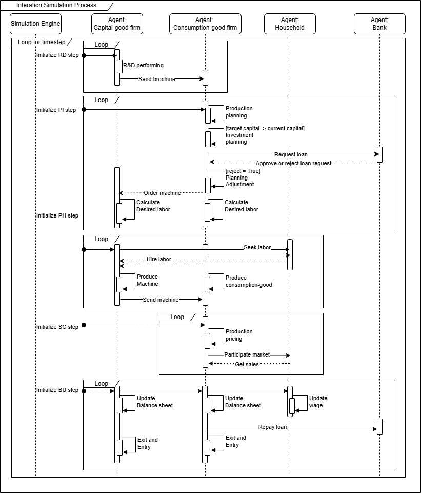
The simulations involve each agent repeating a series of decision steps: 1) Research and Development (RD), 2) Planning and Investment (PI), 3) Production and Hiring (PH), 4) Sale and Consumption (SC), and 5) Balance-Sheet Update (BU). A complete cycle of these five decision steps constitutes one time step and each time step corresponds to a single real-world quarter. Figure 2 shows a sequence diagram of the proposed model. We also provide our code on COMSES: https://www.comses.net/codebases/a7827ec7-4b25-43db-91b1-80bc1f37a0dc/releases/1.0.0/
Research and development (RD) step
The overall process and equations used in this RD step are the same as those in the original K+S model (Dosi et al. 2013); however, we add the assumption that the marginal innovation of technology diminishes as the technological level improves, as in Schumpeterian endogenous growth models (Madsen 2007). We model both the success probability of the R&D process and the actual increase in the technological level to diminish according to this assumption. A detailed explanation of how we modeled them is provided in paragraphs 3.11 and 3.12.
During the RD step, K-firms enhance their technological capabilities through R&D efforts. These firms possess distinctive technological levels, encapsulated by \(A_i\) and \(B_i\). \(A_i\) denotes the machine’s performance, signifying the productivity when the machine combines with labor to produce consumer goods. \(B_i\) represents the productivity of K-firms manufacturing machines.
K-firms invest a proportion of their previous period’s machine sales revenue in R&D. The R&D investment for K-good \(i\) at time \(t\) is determined by the following equation:
| \[RD_i(t)=\nu S_i(t-1) \;\,\, for \;\,\, t \geq 1\] | \[(1)\] |
K-firms pursue R&D through two approaches: innovation (\(IN\)) and imitation (\(IM\)). The allocation of total R&D investment is distributed between the two methods. The investment in each R&D approach is determined as follows:
| \[IN_i(t) = \xi \times RD_i(t), \;\, IM_i(t) = (1-\xi) \times RD_i(t)\] | \[(2)\] |
The success probability of each R&D process is determined by the allocated investments and established technological level. Given the probability of success, the outcome of each process was determined using Bernoulli sampling, as assumed in the K+S model. In addition to the assumption in the original K+S model, where only the allocated investment influences the success probability, we introduce an additional assumption: the higher the established technological level, the lower the success probability. To model this assumption, we calculate the current technological level with the L2 norm for pair \((A_i^\tau , B_i^\tau)\) and divide the allocated investments \(IN_i (t)\) and \(IM_i (t)\). Here,\((A_i^\tau , B_i^\tau)\) represent the established levels of technology from previous timestep as below.
| \[A_i^\tau (t)=A_i(t-1) \;\, for \;\, t \geq 1, \quad B_i^\tau (t)=B_i(t-1)\;\, for \;\, t \geq 1\] | \[(3)\] |
| \[\theta_i^{IN}(t) = 1 - {e^{-\zeta_1 IN_i(t)/\sqrt{(A_i^\tau (t))^2 + (B_i^\tau(t))^2}}},\; \theta_i^{IM}(t) = 1-{e^{-\zeta_2 IM_i(t)/\sqrt{(A_i^\tau(t))^2 + (B_i^\tau(t))^2}}}\] | \[(4)\] |
If the innovation process succeeds, the firm attains a new technological level that increases by a random proportion from its current technological level. We have added the assumption that, in this process, the higher the current technological level, the smaller the increase in the technological level. Again, to model this assumption, we divide the increase in technological level by the current technological level, which is calculated as the L2 norm for pair \((A_i^\tau , B_i^\tau)\). The original K+S model modeled the innovation process as \(A_i^{IN}(t)=A_i^{\tau} (t)(1+{x_i^A(t)})\) and \(B_i^{IN}(t)=B_i^{\tau} (t)(1+{x_i^B(t)})\), where \(x_i^A\) and \(x_i^B\) are randomly sampled from a beta distribution. However, as our model assumes diminishing returns, the new technological level after a successful innovation process is determined by the following formula:
| \[\begin{aligned} A_i^{IN}(t) &= A_i^{\tau} (t)\left(1+\frac{x_i^A(t)}{\sqrt{(A_i^\tau (t))^2 + (B_i^\tau (t))^2}}\right), \\ B_i^{IN}(t) &= B_i^\tau(t)\left(1+\frac{x_i^B(t)}{\sqrt{(A_i^\tau (t))^2 + (B_i^\tau (t))^2}}\right) \end{aligned}\] | \[(5)\] |
If the imitation process succeeds, then the firm acquires the technological level of another randomly selected firm. Here, the selection of the other firm is random, but weighted by technological proximity, denoted by \(W_i\). In other words, a firm is more likely to imitate another firm with a similar technological level to its own. We determine the firm to be imitated, indexed by \(k^*\), as follows:
| \[\begin{aligned} W_i &= (w_{i1}, \ldots, w_{iN_{F_k}}) \quad \text{where} \quad w_{ik} = \begin{cases} \displaystyle \frac{1}{\sqrt{(A_i^\tau(t) - A_k^\tau(t))^2 + (B_i^\tau(t) - B_k^\tau(t))^2}} & \text{for} k \neq i, \\ 0 & \text{for } k = i \end{cases} \\[1em] k^* &= \operatorname*{argmax}_{j \in \{1,2,\ldots,N_{F_k}\}} X_j \quad \text{where} \quad X = (X_1, X_2, \ldots, X_{N_{F_k}}) \sim \text{Multinomial}(1, W_i) \\[0.5em] A_i^{IM}(t) &= A_{k^*}^\tau(t), \qquad B_i^{IM}(t) = B_{k^*}^\tau(t) \end{aligned}\] | \[(6)\] |
After the R&D process concludes, K-firms compare their current technology (\(\tau\)) with technologies obtained from innovation (\(IN\)) and imitation (\(IM\)). They then choose the optimal technology as their final technology, considering both the price (\(p_i\)) of the machine, determined by \(B_i\) and the machine’s performance, determined by \(A_i\). First, we model the price of a machine created from each process, considering the efficiency of producing machines, \(B_i\).
| \[p_i^h(t)=(1+\mu_1)\frac{wage(t)}{B_i^h (t)}, \;\, h\in\{IN,IM,\tau\}\] | \[(7)\] |
| \[\begin{aligned} h^* &=\underset{h}{\arg\min} \,[p_i^h + b \times c(A_i^h (t),t)], \; h \in \{IN, IM, \tau\}\\ &A_i(t) =A_i^{h^*} (t), \quad B_i(t) =B_i^{h^*} (t), \quad p_i(t) =p_i^{h^*} (t) \end{aligned} \] | \[(8)\] |
Finally, K-firms promote their technological capabilities by sending brochures containing information about the prices and productivity of their machines to potential customers (C-firms). The potential customers consist of past and randomly selected customers. The number of new customers (\(NC\)) depends on the number of past customers (\(HC\)), given by
| \[NC_i(t) = max(\gamma HC_i(t), mc-HC_i(t)) \quad where \quad HC_i(0)=0\] | \[(9)\] |
In the market protocol, the price setter in the capital goods market is the supplier, that is, the K-firm. Consumers–namely, consumer goods firms–accept prices as given. Each K-firm applies a markup to the unit cost of producing a single capital good, which is determined by its technological level. The markup rate is uniform across firms and remains constant over time. Thus, firms do not derive additional benefits from markups. Instead, K-firms with superior technology can lower their unit production costs, and consequently, their prices. This allows them to attract larger customer bases through price competition. However, because not all consumer goods firms receive brochures for every capital good, the firm offering the lowest price does not monopolize the entire market.
Planning and investment (PI) step
In the PI step, C-firms formulate a production plan and proceed with capital investments based on this plan. Additionally, in the credit-augmented K+S model, there is an added process in which C-firms secure insufficient funds through financing. The bank agent determines the approval of loan requests from C-firms.
These processes and general equations are the same as those in the original K+S model, but we use the CD function instead of Leontief fixed-proportional function in the K+S model for the production function of a C-firm. Therefore, each firm’s demand for labor and capital investment is calculated differently in our model based on the changed production function, as in Equations 11 and 12.
First, the target production levels of(\(Q^T_j\)) C-firms are determined based on the expected demand (\(D^e_j\)) and target inventory levels (\(N^T_j\)). Each value is formalized using the following equations:
| \[\begin{aligned} Q_j^T(t) = D_j^e(t)+N_j^T(t)-N_j(t-1) \;\,where \,\; D_j^e(t)=D_j(t-1)\;\, and\;\,N_j^T(t)=\iota D_j^e(t) \quad for \;\, t \geq 1 \;\, \end{aligned}\] | \[(10)\] |
To achieve their target production levels, C-firms determine the necessary amount of labor based on their current capital. In traditional economic equilibrium models, firms typically choose optimal amounts of capital and labor to meet their production targets, considering wages and the prices of capital goods. However, in reality, a time delay exists between ordering and receiving a capital good. In other words, investment in capital goods is only reflected in a firm’s total capital in the following period: Consequently, C-firms must determine their required labor based on their existing machinery. This target level of labor is denoted as \(L_j^T(t)\) and formulated as follows:
| \[L_j^T(t) = \left( \frac{Q_j^T(t)}{A_j^{avg}(t) \times K_j (t)^\alpha} \right)^\frac{1}{1-\alpha} \quad where \quad A_j^{avg}(t) = \frac{\sum_{k=1}^{K_j(t)}A_j^k(t)}{K_j(t)} \] | \[(11)\] |
Next, C-firms create capital investment plans to acquire machines from K-firms. The C-firm firm chooses its preferred machines from the brochures received at this time step and purchases the machines from the corresponding K-firm. Preferred products refer to those with the lowest value according to Equation 8.
Capital investments can be divided into expansion and replacement. In the expansion process, C-firms aim to optimize the ratio of labor to capital by expanding their machine capacity. The optimal amount of capital is achieved when the marginal product of labor equals the marginal product of capital for an additional unit of money spent. Therefore, our model remodeled each firm’s optimal capital level \(K_j^*(t)\) as follows:
| \[K_j^*(t) = \frac{\alpha \times \eta \times wage(t) \times A_j^*(t) \times L_j^T(t)}{(1-\alpha) \times p_j^*(t) \times A_j^{avg}(t)} \] | \[(12)\] |
Notably, labor demand for the next time step decreases when wages increase, through Equation 12. When wages increase relative to the cost of capital, the optimal capital investment level increases. Consequently, the firm requires less labor in the next time step due to the increased availability of capital, leading to a reduction in labor demand. Thus, labor demand decreases as wages increase in our market protocol.
However, to prevent ordering an excessive number of machines, the number of machines that could be expanded simultaneously was constrained. The expansion upper limit is set below a certain percentage of the existing capital. Consequently, the final target amount of additional capital for expansion, \(EI_j^T(t)\), is defined by the following equation:
| \[EI_j^T(t) = \min \left( K_j^*(t) - K_j(t), \, \delta K_j(t) \right)\] | \[(13)\] |
In the replacement process, C-firms replace machines that significantly underperform compared to the latest products or have reached the end of their lifespan (\(\eta\)). Machines are considered candidates for replacement if they meet the following conditions: substantial performance degradation. Consequently, the final target amount of additional capital for replcaement, \(RS_j^T(t)\) is defined as follows:
| \[RS_j^T(t) = \left| \left\{ k \in \Xi_j(t) \bigg| \frac{p_j^*(t)}{c(A_j^k(t),t) - c(A_j^*(t),t)} \leq b \; and \; c(A_j^k(t),t) \ge c(A_j^*(t),t),\;\, or \;\, age_j^k(t) > \eta \right\} \right|\] | \[(14)\] |
| \[K_j^T(t)=EI_j^T(t)+RS_j^T(t)\] | \[(15)\] |
After formulating plans for production and capital investment, C-firms assess the financial feasibility of their plans. If the firm can employ the required amount of labor and expand (or replace) capital with current liquidity, there is no issue. However, if this is not feasible, C-firms request financing from banking agents. The necessary credit demand is
| \[CD_j^e(t) = \max \left( 0, wage(t) \times L_j^T(t) + p^*_j \times K_j^T(t) - NW_j(t) \right)\] | \[(16)\] |
The bank agent determines the approval of loan requests from C-firms. Initially, the bank decides on the amount of total credit to supply in the market based on the firms’ liquidity, following the formula below:
| \[MTC(t) = k \left( \sum_{i=1}^{N_{F_K}}{NW_i(t)} + \sum_{j=1}^{N_{F_C}}{NW_j(t)} \right)\] | \[(17)\] |
Subsequently, the bank agent assesses loan requests, starting with firms that exhibit high sales, thereby favoring those with stronger performance. For each firm, the bank considers the DSR and remaining credit to determine whether to approve the loan and the loan amount. The loan amount for firm \(j\) is determined using the following equation:
| \[CD_j(t) = \min \, ( CD_j^e(t), \; \lambda \times S_j(t-1) - debt_j(t), \; MTC(t) - \sum_{j=1}^{N_{F_C}}{debt_j(t)} )\] | \[(18)\] |
Finally, C-firms adjust their production and investment plans based on approved loan amounts. In this process, firms prioritize maintaining workforce employment over investing in it. Consequently, firms facing financial constraints first reduce their investment levels and subsequently reduce their employment. Therefore, the final labor demand of firm \(j\), \(L_j^d(t)\) and final capital demand, \(K_j^d(t)\), are formalized as follows:
| \[\begin{aligned} L_j^d(t) &= \min \left( L_j^T(t), \, \frac{NW_j(t)+CD_j(t)}{wage(t)} \right)\\ K_j^d(t)=min&\left(K_j^T(t), \, \frac{NW_j(t)+CD_j(t)-wage(t) \times L_j^d(t)}{p_j^*(t)}\right) \end{aligned}\] | \[(19)\] |
Then, the production demand for K-firm \(i\), \(Q_i^d(t)\), is the total amount of machines ordered by C-goods firms targeting it. To meet demand within its liquidity, \(NW_i(t)\), K-goods firm \(i\) requires labor, \(L_i^d(t)\), as follows:
| \[L_i^d(t)=min\left( \frac{Q_i(t)}{B_i(t)}, \frac{NW_i(t)}{wage(t)}\right)\] | \[(20)\] |
Production and hiring (PH) step
In the PH step, we follow the original K+S model and equations; however, in our model, we use the CD function as the production function of each C-firms, as mentioned above. This causes a difference in Equation (22).
In this step, both the K- and C-firms hire as much labor as possible up to their demand. Because all households wish to be employed, the total labor supply equals the number of households, \(N_H\). If the overall labor demand across all sectors is lower than the available labor supply (\(N_H\)), then the final labor employment for each firm \(L^h\) equals the required labor amount. Conversely, if the total employment demand \(L^D\) surpasses labor supply, firms uniformly reduce their final labor employment from the required labor amount. The following formulas are used to ascertain the final labor employment for each firm:
| \[L^h(t) = \lfloor L^d (t)\times \frac{N_H}{L^D(t)} \rfloor \quad where \quad L^D(t) = \sum_{i=1}^{N_{F_K}}{L_i^d(t)} + \sum_{j=1}^{N_{F_C}}{L_j^d(t)}\] | \[(21)\] |
Next, based on the determined labor employment, firms initiate production of their products. The production quantity of each firm is
| \[Q_i(t) = L_i^h(t) \times B_i(t), \;\; Q_j(t) = A_j^{avg}(t) \times K_j (t)^\alpha \times L_j^h(t)^{1-\alpha}\] | \[(22)\] |
| \[K_j^s(t)=K_j^d(t) \times \min \left( \frac{Q_{\overline{j}}(t)}{Q_{\overline{j}}^d(t)},1 \right) \;\,and\;\, K_j(t+1)=K_j(t)+K_j^s(t)\] | \[(23)\] |
| \[N_j(t)=N_j(t-1)+Q_j(t)\] | \[(24)\] |
Sale and consumption (SC) step
For the SC step, we follow the update rules for markup, competitiveness, and market share of the K+S model, as in Equations (25), (27), and (28), respectively. In addition, the equations for the product price of each C-firm, the total consumption, and the demand and revenue of each firm are derived based on the description written in the K+S model.
During this step, C-firms set prices for their products, and the firms’ final revenue is determined based on these prices. The K+S model relies on the assumption of markup pricing. To establish the price of the consumption good, the initial step involves determining the markup rate. The markup rate (\(\mu_j\)) is specific to each C-goods firm and is determined as follows, considering the market share trend (\(f_j\)) from previous time steps6
| \[\mu_j(t) = \mu_j(t-1) \times \left( 1 + \rho \times \frac{f_j(t-1) - f_j(t-2)}{f_j(t-2)}\right) \quad for \quad t \geq 2 \] | \[(25)\] |
Firms determine the final price of a consumption good based on a predetermined markup rate and production cost of the product. To simplify the model, the production cost only considers the cost of labor (wages), and the depreciation cost of capital is incorporated into the markup rate. In summary, the final product price for C-firms is
| \[p_j(t) = \frac {(1+ \mu_j(t)) \times L_j^h \times wage(t) + N_j(t-1) \times p_j(t-1)}{Q_j(t) + N_j(t-1)}\] | \[(26)\] |
Next, to determine the revenue of C-firms, the market competitiveness (\(E_j\)) of each firm is calculated. A firm’s market competitiveness is assessed on the basis of the following two factors: First, given our assumption that goods are homogeneous, lower-priced products are more competitive. Second, the unfilled demand from the previous time step is considered. From the consumer’s perspective, this reflects how well a firm predicts demand and supplies an adequate quantity of the product. In summary, a firm’s competitiveness is determined through the following equation7
| \[E_j(t) = -\omega_1 p_j(t) -\omega_2 l_j(t-1) \quad for \quad t \geq 1 \] | \[(27)\] |
The market share of each firm was determined based on its market competitiveness. Comparing a firm’s market competitiveness with the average market competitiveness of C-firms, we increase the market share of firms with higher competitiveness and decrease the market share of those with lower competitiveness. The market share update formula is as follows:8
| \[\begin{aligned} f_j(t)=\frac{\overline{f_j}(t)}{\sum_{j'=1}^{N_{F_C}}\overline{f_{j'}}(t)}& \quad where \,\ \overline{f_j}(t) = f_j(t-1) \times \left( 1 + \mathcal{X} \times \frac{E_j(t) - \overline{E}(t)}{\overline{E}(t)} \right)\\ and& \,\ \overline{E}(t) = \sum_{j'=1}^{N_{F_C}}f_{j'}(t-1) \times E_{j'}(t) \,\; for \,\ t \geq 1\\ \end{aligned} \] | \[(28)\] |
Finally, the firms determine their ultimate revenue based on their market share. Household agents consume all wages earned through labor and the entire unemployment subsidy at this time step. The unemployment subsidy is set as a fixed percentage of wages. Therefore, total consumption is calculated as
| \[C(t) = L^D(t) \times wage(t) + (L^S - L^D(t)) \times \phi \times wage(t)\] | \[(29)\] |
Reflecting the market share of C-firms, total consumption is allocated to the demand for firms’ products. C-firms determine their final revenue based on the demand for products (\(D_j(t)\)) and current inventory (\(N_j(t)\)). If inventory is insufficient to meet product demand, then we treat it as unfilled demand, which adversely affects future market competitiveness. In summary, the product demand and final revenue of firms are determined using the following equations:
| \[D_j(t) = \lceil C(t) \times \frac{f_j(t)}{p_j(t)}\rceil, \;\; S_j(t) = \min {\left( D_j(t),\; N_j(t)\right)} \times p_j(t)\] | \[(30)\] |
Balance-sheet update (BU) step
The equations used in the BU step follow those used in the K+S model. In this BU step, the final profits of firms in both sectors are calculated and corporate taxes and bank repayments are reflected in their liquidity. Additionally, market indicators such as average labor productivity and the unemployment rate are computed, and based on these, wages are updated. Finally, the firms experience market exits and entries.
First, K-firms calculate their profits (\(\Pi_i\)) by subtracting R&D investment and the cost of machine production from the revenue generated by selling machines. Next, they receive interest in their deposit, apply corporate taxes to profits, and update liquidity as follows:
| \[\begin{aligned} &\Pi_i(t) = S_i(t) - wage(t) \times L_i^h(t) - RD_i(t), \\ &NW_i(t+1) = NW_i(t) + NW_i(t) \times r_d + (1-tr) \times \Pi_i(t) \quad where \quad r_d=\frac{(1-\pi_d)\times r}{4} \end{aligned}\] | \[(31)\] |
C-firms calculate profits by subtracting the capital investment and production costs of goods from the revenue generated by selling consumption goods. For the loan repayments, we assume that the bank uses the equal principal and interest payment method. As with K-firms, they receive interest on their deposits, pay corporate taxes, repay the principal and interest on the loan, and update their liquidity, as follows:
| \[\begin{aligned} &\Pi_j(t) = S_j(t) - wage(t) \times L_j^h(t) - p_j^* \times K_j^s(t), \\ &NW_j(t+1) = NW_j(t) + NW_j(t) \times r_d + (1-tr) \times \Pi_j(t) - loanRepayment_j(t)\quad where\\ &loanRepayment_j(t)=debt_j(t) \times r_l \times \frac{(1+r_l)^{pr}}{(1+r_l)^{pr}-1} \quad where \quad r_l=\frac{(1+\pi_u)\times r}{4} \end{aligned}\] | \[(32)\] |
Here, \(r_l\) represents the quarterly interest rate on the loan considering the bank markup rate, \(\pi_u\).
Next, market indicators such as the average labor productivity (AB) and employment rate(EM) are calculated. Both indicators were updated using the following equations:
| \[\begin{aligned} &AB(t) = \frac{\sum_{j=1}^{N_{F_C}}Q_j(t)}{(\sum_{j=1}^{N_{F_C}}K_j(t))^\alpha (\sum_{i=1}^{N_{F_K}}L_i^h(t) + \sum_{j=1}^{N_{F_C}}L_j^h(t))^{1-\alpha}} \\ &EM(t) = \frac{\sum_{i=1}^{N_{F_K}}L_i^h(t) + \sum_{j=1}^{N_{F_C}}L_j^h(t)}{N_H} \end{aligned}\] | \[(33)\] |
For real wages, a decrease in labor productivity or the employment rate reduces the value of hiring labor, leading firms to lower wage levels. Accordingly, the wage is updated as follows:
| \[wage(t+1) = wage(t) \times (1+ \psi_1 \frac{AB(t) - AB(t-1)}{AB(t-1)} + \psi_2 \frac{EM(t) - EM(t-1)}{EM(t-1)}\quad for \quad t\geq 1\] | \[(34)\] |
| \[N_j(t)=max(Q_j(t)-D_j(t),0)\] | \[(35)\] |
Finally, firms with low competitiveness exit and new firms enter. Assuming a fixed number of firms, an equal number of new firms enter the market. For K-firms, exit occurs if there are no product sales for three consecutive periods. C-firms, will consider an exit if there is no demand or if they cannot engage in production because they lack capital or liquidity. The exit processes for both firms can be formulated as follows:
| \[\begin{aligned} &K-firm\quad i \quad exits \quad if\quad S_i(t)=S_i(t-1)=S_i(t-2)=0\\ &C-firm\quad j \quad exits\quad if\quad NW_j(t)<0\quad or\quad D_j(t)=0\quad or\quad K_j(t)=0 \end{aligned}\] | \[(36)\] |
Output Validation
Prior to performing the experiments with our model, we validated it by comparing the simulation results with real data. We used South Korea’s historical data spanning three decades (1991-2020), encompassing 120 quarters. The validation targets were chosen based on three aspects: output, capital, and labor. To address the gap between the simulation model and the real world, each validation dataset was scaled to be the same as the corresponding simulation results at one reference time. The first quarter of 1991 served as the reference time for Log Real GDP, whereas the first quarter of 2010 was the starting point for the equipment investment index, employment rate, and wages. Detailed information on the validation data and corresponding simulation outputs is summarized in Table 1.
| Division | Historical Data | Data Source | Sampling Period | Simulation Output |
|---|---|---|---|---|
| Output | Real GDP | Bank of Korea | 1991-2020 | Total consumption good output |
| Capital | Equipment Investment | Statistic Korea | 1995-2020 | Consumption-goods firms’ investment |
| Index | ||||
| Labor | Employment Rate | Statistic Korea | 1999-2020 | Employment rate |
| Hiring Rate | OECD | 2000-2020 | Employment rate | |
| Wage | Korean Ministry of | 2006-2020 | Wage | |
| Employment Labor | ||||
The simulation results for each validation target are averaged over 50 replicates. Over 170 timesteps from the results, we used data from the last 120 timesteps, each of which corresponded to one-quarter in the real world. During the discarded first 50 timesteps, each firm, with randomly sampled capital and assets at the beginning, grows into an enterprise of a specific size, constructing a realistic industrial organization in the model. Also, the output data tend to stabilize after this burn-in period of 50 timesteps, as shown in Appendix B. The entire parameter list of our model is presented in Table (???). We use the same values as Dosi’s model (Dosi et al. 2013) for those that did not undergo calibration.
The validation results showed consistent matching in trends between each simulation and validation data, as shown in Figure 3. To evaluate our model quantitatively, the Mean Average Percentage Error (MAPE) served as the performance measure. The MAPE for each validation target is shown in each subfigure of Figure 3. All of these values were less than 15%. This result implies that our model performs well under the current assumptions and effectively captures historical data trends.
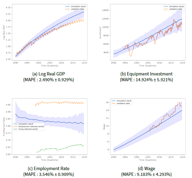
When validating for GDP, we used the logarithm of real GDP, as illustrated in Figure 3a. This is because when the absolute change is small, taking the logarithm allows for a more detailed understanding of the trend as it amplifies relative changes on a finer scale. For calculating the MAPE of employment rate, we use two different references for the validation data to calculate the MAPE of the employment rate. In the real economy, the employment rate refers to the proportion of people who are employed out of the labor force, while the hiring rate refers to the proportion of employed individuals within the total population. Since the labor force is a subset of the total population, the employment rate is typically higher than the hiring rate. In contrast to the real world, our model assumes that no households drop out of the labor force and all are willing to work, so the total population is equivalent to the labor force. As a result, the employment rate in our model is expected to fall between the real-world employment rate and the hiring rate. To bridge this gap, we use the average of the two real-world rates as a benchmark in our fitness calculation.
| Symbol | Description | Value | Calibrated |
|---|---|---|---|
| \(\zeta_1\) | Innovation success rate | 0.3 | Y |
| \(\zeta_2\) | Imitation success rate | 0.32 | Y |
| \((\alpha_1, \beta_1)\) | Beta distribution parameter for innovation | (3,3) | Y |
| \((\underline{X},\overline{X})\) | Beta distribution support for innovation | (-0.2,0.35) | Y |
| \(\mu_1\) | Mark-up coefficient (capital) | 0.18 | Y |
| \(\mu_0\) | Mark-up coefficient (consumption) | 0.57 | Y |
| \(\rho\) | Mark-up rule coefficient | 0.06 | Y |
| \(\iota\) | Desired inventory level | 0.2 | Y |
| \(\delta\) | Maximum capital expansion rate | 0.2 | Y |
| \(DSR\) | Maximum debt to sales ratio | 2 | Y |
| \(\psi_1\) | Wage coefficient for labor productivity | 0.89 | Y |
| \(\psi_2\) | Wage coefficient for unemployment rate | 0.14 | Y |
| \(\omega_1\) | Competitiveness coefficient for price | 0.7 | Y |
| \(\omega_2\) | Competitiveness coefficient for unfilled demand | 0.35 | Y |
| \(\chi\) | Replicator dynamics coefficient | 0.06 | Y |
| \(\upsilon\) | Initial employment rate | 0.66 | Y |
| \(mc\) | Minimum client | 5 | Y |
| \(\gamma\) | New client sampling rate | 0.04 | Y |
| \(k\) | Credit multiplier | 4 | N |
| \(N_{Fk}\) | Number of capital-goods firm agents | 50 | N |
| \(N_{Fc}\) | Number of consumption-goods firm agents | 200 | N |
| \(N_H\) | Number of Household agents | 3000 | N |
| \(T\) | Maximum simulation run time | 120 | N |
| \(\nu\) | R&D investment propensity | 0.04 | N |
| \(\xi\) | R&D allocation to innovative process | 0.5 | N |
| \(b\) | Payback period | 3 | N |
| \(\eta\) | Physical scrapping age | 20 | N |
| \(\alpha\) | Cobb-douglas alpha | 0.3 | N |
| \(r\) | Interest rate | 0.025 | N |
| \((\pi_u, \pi_d)\) | Mark up and down for interest rates on deposits and loans | (0.5,1) | N |
| \(pr\) | Loan principle repayment rate (maturity) | 20 | N |
| \(tr\) | Tax rate | 0.1 | N |
| \(\phi\) | Unemployment subsidy rate | 0.4 | N |
| \(NW^{init}\) | Initial average liquidity of firms | 50 | N |
| \(A^{avg}\) | Initial average machine performance | 1 | N |
| \((\alpha_2, \beta_2)\) | Beta distribution parameter for new entrants’ technological level | (4,2) | N |
Policy Experiment
The objective of the policy experiment was to analyze the effects of financial policies on market concentration, economic growth, and labor income share. For financial policies, we chose the upper limit of DSR and the interest rate, which regulate the quantity and cost of finance, respectively. To facilitate a direct comparison of the effects of the DSR limit and interest rates, the experimental results in the following sections are consistently analyzed in the direction where more financing is provided: an increase in the DSR limit and a decrease in the interest rate.
For proxies of market concentration, economic growth, and labor income share, we use the Herfindahl-Hirschman Index (HHI), the real GDP growth rate, and the labor income share as a proportion of total income, respectively. The HHI is defined as the sum of the squared values of the market share of C-firms. Real GDP was calculated as the sum of the total production of consumption goods. The labor income share is measured as the proportion of nominal wages paid to households employed by C-firms out of the total nominal value of the production of consumption goods. We performed both descriptive and regression analyses to investigate the effects of financial policies on the three dependent variables. For the regression analysis, the dependent variables were HHI, economic growth, and labor income share, while the independent variables were financial policy variables.
Table 3 summarizes the experimental design of the policy experiment for RQ 1 and RQ 2 regarding the sampling of the policy variables. ‘Exp 1’ and ‘Exp 2’ are descriptive analyses that examine the impact of a single financial policy change. For each financial policy, 300 values were sampled, whereas the other financial policy was fixed at the same value used in the output validation. When the DSR limit is sampled for 300 times, the interest rate is fixed as 0.025 and we denote this experiment as ‘Exp 1’. Conversely, when the interest rate is sampled for 300 times, the DSR limit is fixed as 2 and we denote this experiment as ‘Exp 2’. Our model was simulated using 20 replicates per value. The HHI, GDP growth rate, and labor income share were averaged over these 20 replications. Also, we utilized these output data from the last period of the simulations. In the case of ‘Exp 3,’ it is a joint regression analysis where both variables change simultaneously. A total of 2500 (DSR, r) combinations were sampled at regular intervals within the sampling range and 20 simulation replications were conducted for each sample. The outcomes were averaged across these replicates and the values during the final simulation period were used. The notations, ‘Exp 1,’ ‘Exp 2,’ and ‘Exp 3’ are consistently used in RQ 1 and RQ 2 to denote the same experiment settings. The following three subsections demonstrate how each outcome changes with the alteration in the two different financial policies.
| Experiment | Policy Variables | Sampling Range | Number of Policy Samples | Number of Replications |
|---|---|---|---|---|
| Descriptive Analysis | ||||
| Exp 1 | Debt-to-Sales Ratio | DSR \(\sim\) Unif [1, 8] | 300 DSR samples | 20 replications for each sample |
| (DSR) | (20 * 300 = 6000 replications) | |||
| Exp 2 | Interest Rate | r \(\sim\) Unif [0.01, 0.1] | 300 r samples | 20 replications for each sample |
| (r) | (20 * 300 = 6000 replications) | |||
| Regression Analysis | ||||
| Exp 3 | DSR, \(~\) r | (DSR,\(~\) r) \(\sim\) Unif [1, 8] \(\times\) Unif [0.01, 0.1] | 2500 (DSR,r) samples | 20 replications for each sample |
| (20 * 2500 = 50000 replications) | ||||
RQ 1. The impact of finance on market concentration
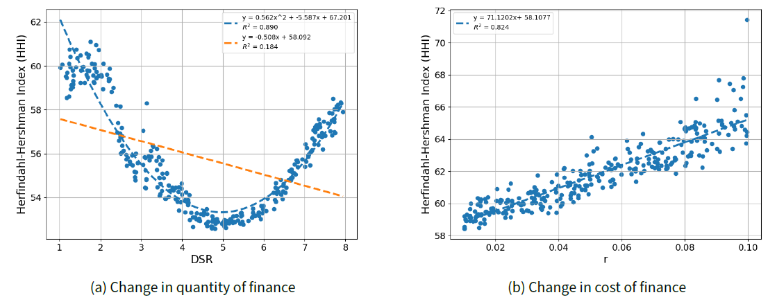
In this subsection, we investigate how HHI changes with variations in DSR values and interest rates in the ‘Exp 1’ and ‘Exp 2’ setups from Table 3, respectively. The results are presented in Figures 4a and 4b. The impact of financing on market concentration varies depending on the policy type. As shown in Figure 4 b, a decrease in the interest rate (r) leads to a decline in the HHI, suggesting that financing facilitated by an expansionary financial policy reduces market concentration and promotes the growth of small firms. By contrast, the DSR limit exhibits a nonlinear relationship with market concentration, as illustrated in Figure 4a. The HHI decreased when the DSR limit was below 5 but increased when it exceeded 5, forming a U-shaped trend. This implies that relaxing the DSR limit to a certain level promotes the growth of small firms more than that of large firms. However, if DSR regulation is excessively loosened, resulting in an excessive quantity of financing flowing into the market, large firms will increasingly dominate as the regulation is eased. The reasoning behind these nonlinear trends in market concentration is closely examined through the firm-level analysis provided in Subsection RQ1-1. How are financing allocated to firms?.
We also conducted statistical tests using the joint regression models below to analyze the impact of financial policies on HHI. For the regression, DSR and interest rates are simultaneously sampled, as in the ‘Exp 3’ setup of Table 3. \(HHI_i, DSR_i\) and \(r_i\) represent HHI, DSR limit, and the interest rate, respectively, for policy case \(i\). The baseline model for the regression is represented by Equation 37.
| \[HHI_i = \beta_0 + \beta_1 \times r_i + \beta_2 \times DSR_i + \epsilon_i \] | \[(37)\] |
| HHI | ||||
| (a) | (b) | (c) | (d) | |
| Constants | 55.304\(^{***}\) | 66.896\(^{***}\) | 58.133\(^{***}\) | 69.725\(^{***}\) |
| (0.218) | (0.215) | (0.373) | (0.270) | |
| \(r\) | 41.268\(^{***}\) | 41.268\(^{***}\) | -10.173\(^{*}\) | -10.173\(^{***}\) |
| (2.587) | (1.541) | (6.109) | (3.524) | |
| \(DSR\) | -0.142\(^{***}\) | -6.663\(^{***}\) | -0.771\(^{***}\) | -7.292\(^{***}\) |
| (0.033) | (0.099) | (0.075) | (0.102) | |
| \(DSR^2\) | 0.725\(^{***}\) | 0.725\(^{***}\) | ||
| (0.011) | (0.010) | |||
| \(r * DSR\) | 11.431\(^{***}\) | 11.431\(^{***}\) | ||
| (1.234) | (0.712) | |||
| Observation | 2500 | 2500 | 2500 | 2500 |
| R-squared | 0.098 | 0.68 | 0.128 | 0.71 |
| Adj.R-squared | 0.098 | 0.68 | 0.127 | 0.71 |
As shown in Table 4, in model (d), in addition to r and DSR, the coefficients of \(DSR^2\) and the interaction term between r and DSR are significant. The significance of \(DSR^2\) supports the nonlinear relationship between DSR and HHI. This indicates that, unlike interest rates, where more financing consistently favors the growth of small firms, DSR exhibits a tipping point beyond which it becomes more advantageous for large firms. Furthermore, the positive significance of the interaction term between r and DSR indicates that the combined effect of these two variables is amplified compared with their individual effects. Specifically, when the interest rate is higher, the effect of relaxing DSR regulations on increasing the HHI becomes more pronounced. A more detailed representation of how HHI changes when both variables change together is provided in the visual heatmap in Appendix C.
RQ 1-1. How is financing allocated among different firms?
This subsection examines how financing is supplied to firms of different sizes as the DSR limits change. This micro-level approach aims to thoroughly analyze the rationale behind the macro-level nonlinear trends in market concentration, as discussed earlier.
We conducted a firm-level analysis to investigate each firm’s loan acquisitions. To compare the different scenarios of DSR regulations, we selected three distinct levels of the DSR limit—2, 5, and 8—for the simulation. These levels were chosen because the HHI exhibited a U-shaped trend around a DSR value of 5 in the experiment for RQ 1. For each scenario, all parameter values remained consistent with those in Table 2, except for the DSR regulation level. We did not replicate the analyses across simulations because the sizes of the firms varied with each replication. Instead, we tracked the sales and debt of each of the 200 C-firms in the last timestep of a single simulation run.
In Figure 5, we illustrate the amount of debt for each C-firm under three scenarios, examining how the amount of debt varies based on the firm’s sales in each scenario. In each scenario, the maximum available debt for each firm based on its sales under the given DSR limit is depicted as a gray dotted line in the figure. As shown in Figure 5a, most firms succeed in acquiring the maximum possible amount of debt based on their sales for DSR limits of two and five. However, Figure 5b demonstrates different results under a DSR limit of 8 compared with those under a DSR limit of 2. Under the DSR limit of eight, large firms do not secure loans for the maximum possible amount. This reflects the situation where DSR regulation is exceptionally relaxed, resulting in the desired loan amounts for each large firm being more than adequately fulfilled. On the contrary, extremely small firms that fall behind in loan priority acquire little debt or even none from the bank. This illustrates a situation in which credit is concentrated in large firms.
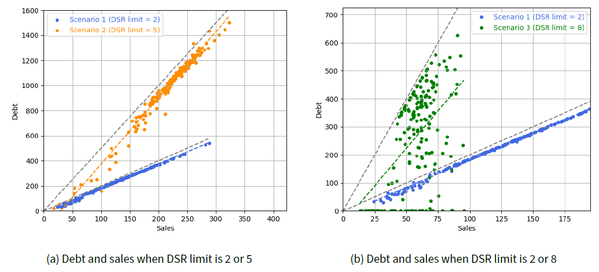
We also conducted statistical tests using the following linear regression model for the three different scenarios. This regression analysis is to analyze how the amount of loans each firm borrows varies based on sales under different levels of DSR regulations. The regression model for firms’ debt and sales is given in Equation 38, where index \(i\) indicates each of the 200 C-goods firms.
| \[Debt_i=\beta_0 + \beta_1 \times Sales_i+\epsilon_i, \quad i=1,2,...200 \] | \[(38)\] |
| Sales | ||||
| Scenario 1 (DSR limit=2) | Scenario 2 (DSR limit=5) | Scenario 3 (DSR limit=8) | ||
| Constants(\(\beta_0\)) | \(-13.224^{***}\) | \(-154.606^{***}\) | \(-44.439\) | |
| \((1.045)\) | \((12.845)\) | \((39.855)\) | ||
| Sales(\(\beta_1\)) | \(1.937^{***}\) | \(5.279^{***}\) | \(5.358^{***}\) | |
| \((0.008)\) | \((0.058)\) | \((0.662)\) | ||
| Observation | 200 | 200 | 200 | |
| R-squared | 0.997 | 0.977 | 0.251 | |
In summary, we find that excessive easing of DSR regulations can create unfair opportunities for firms based on sales. It can concentrate financial resources on large firms and exacerbate market polarization among them. This explains the increasing trend of HHI in Figure 4a when the DSR limit surpasses five.
RQ 2. The impact of finance on economic growth and labor income share
In this subsection, we analyze the effect of financing on economic growth and the labor income share. We examined how each financial policy, while exerting specific effects on market concentration, generates side effects on growth and income distribution, which are closely related to market concentration. Descriptive and regression analyses were performed for each variable. Through these analyses, we compared our findings with those of previous studies to assess consistency. Moreover, we offer implications of the impact of financial policies on market concentration, economic growth, and income distribution.
The impact of finance on economic growth
Figure 6 illustrates how the GDP growth rate changes for each financial policy type. We sample DSR limits or interest rates with the ‘Exp 1’ and ‘Exp 2’ setups from Table 3, respectively. From Figure 6a, the GDP growth rate increases when DSR limit is relaxed. In addition, as shown in Figure 6b, the GDP growth rate increases as interest rates decrease. These results demonstrate that expansionary financial policies foster economic growth, regardless of whether they regulate the quantity or cost of finance. This finding also coincides with the traditional view in existing literature that financing facilitates economic growth.
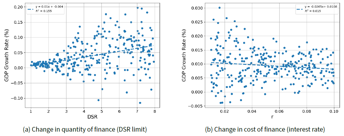
We also conduct statistical tests using the joint regression models below to analyze the impact of financial policies on economic growth. \(GDP_i, DSR_i\) and \(r_i\) represent GDP growth rate, DSR limit and interest rate at each policy case \(i\), sampled as in Table 3 ‘Exp 3.’ The baseline model for the regression is represented by formula 39.
| \[GDP_i = \beta_0 + \beta_1 \times r_i + \beta_2 \times DSR_i + \epsilon_i \] | \[(39)\] |
The regression results are presented in Table 6. The overall variance is high for the economic growth rate, leading to lower R-squared values and reduced explanatory power of the models. However, two interpretations can be drawn from regression analysis. First, low interest rates promote economic growth. The coefficient of r is negative in Models (a) and (b), whereas it is positive in Models (c) and (d). However, this finding does not support the hypothesis that higher interest rates foster economic growth. In Models (c) and (d), the interaction term between r and DSR is significantly negative, suggesting that when DSR is high, the adverse effect of rising interest rates on growth becomes more pronounced. Second, DSR has a nonlinear effect on economic growth. In complex model (d), where all coefficients are statistically significant, the coefficient of DSR is positive, whereas the coefficient of \(DSR^2\) is significantly negative. This indicates that an increase in DSR may eventually slow economic growth. Such effects were not readily observed in the analysis in which only DSR varied while r was fixed, as shown in Figure 6b. Nevertheless, these two interpretations are explored in greater detail in the heatmap in Appendix C, where both financial policies vary simultaneously.
| Economic Growth Rate | ||||
| (a) | (b) | (c) | (d) | |
| Constants | 0.01\(^{***}\) | -0.015\(^{***}\) | -0.007 | -0.033\(^{***}\) |
| (0.003) | (0.005) | (0.005) | (0.006) | |
| \(r\) | -0.092\(^{***}\) | -0.092\(^{***}\) | 0.223\(^{***}\) | 0.223\(^{***}\) |
| (0.033) | (0.033) | (0.079) | (0.078) | |
| \(DSR\) | 0.005\(^{***}\) | 0.020\(^{***}\) | 0.009\(^{***}\) | 0.023\(^{***}\) |
| (0.000) | (0.002) | (0.001) | (0.002) | |
| \(DSR^2\) | -0.002\(^{***}\) | -0.002\(^{***}\) | ||
| (0.000) | (0.000) | |||
| \(r * DSR\) | -0.07\(^{***}\) | -0.07\(^{***}\) | ||
| (0.016) | (0.016) | |||
| Observation | 2500 | 2500 | 2500 | 2500 |
| R-squared | 0.06 | 0.078 | 0.067 | 0.085 |
| Adj. R-squared | 0.059 | 0.077 | 0.066 | 0.084 |
The impact of finance on labor income share
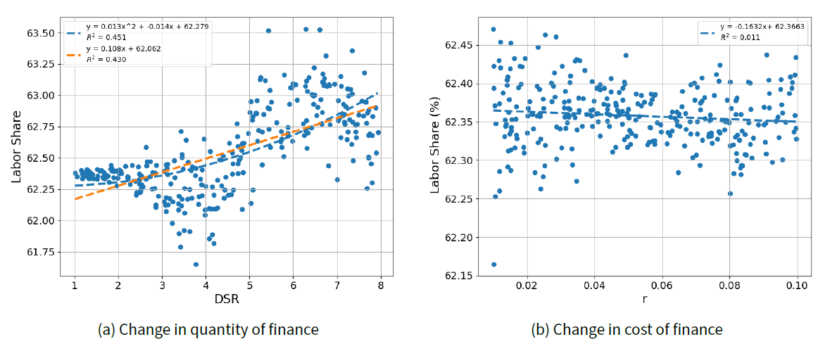
The effect of financing on labor income share varies depending on the type of policy. We sample DSR limits or interest rates with the ‘Exp 1’ and ‘Exp 2’ setups from Table 3, respectively. Figure 7 illustrates how the labor income share changes with each financial policy. The labor income share has a nonlinear relationship with DSR limit, as depicted in Figure 7 a. In contrast, when interest rate r decreases, the labor income share increases, as shown in Figure 7 b.
These results are in line with the impact of financing on market concentration analyzed in RQ 1. The literature suggests that market concentration and labor income share generally have a negative correlation (Akcigit & Ates 2021b). In our experiment, both HHI and labor share exhibited nonlinear trends with changes in the DSR limit, and their directions appeared to be opposite. However, while HHI followed a U-shaped trend as the DSR limit increased, labor share did not exhibit a precisely inverted U-shape. This discrepancy may arise because previous studies asserting a negative correlation between HHI and labor share did not account for financial factors, whereas our analysis considers their relationship within the context of changing financial policies.
We also conducted statistical tests with the joint regression models below to analyze the impact of financial policies on the labor income share. \(LS_i, DSR_i\) and \(r_i\) represent the labor income share, DSR limit and interest rate at each policy case i, sampled as in ‘Exp 3’ setups from Table 3. The baseline regression model is represented by formula 40.
| \[LS_i = \beta_0 + \beta_1 \times r_i + \beta_2 \times DSR_i + \epsilon_i \] | \[(40)\] |
First, regarding the interest rates in Models (a) and (b), the coefficient of r is negative, consistent with the results of the descriptive analysis. However, in Model (d), the coefficient r is positive. Nonetheless, the interaction term between r and DSR in model (d) has a negative coefficient, indicating that when DSR is high, an increase in interest rates leads to a decline in the labor income share. Therefore, we conclude that, in general, higher interest rates tend to reduce the labor income share, which aligns with the findings of a previous descriptive analysis. Next, regarding DSR, its effect on the labor income share appears to be nonlinear. In model (d), the coefficient of the first-order term is positive, suggesting that an increase in DSR raises the labor income share to a certain level. However, the coefficient of the second-order term is significantly negative, indicating that beyond a certain threshold, further increases in DSR may lower labor income share. This result is consistent with the findings in Figure 7 a. Additionally, observing the signs of the coefficients, it can be confirmed that financing has an effect on the labor income share, which is opposite to its effect on market concentration. The heatmap of the changes in labor income share resulting from the joint variations in these two financial variables is provided in Appendix C. This heatmap result more clearly highlights the negative correlation between market concentration and labor income share.
| Labor Income Share | ||||
| (a) | (b) | (c) | (d) | |
| Constants | 62.545\(^{***}\) | 61.758\(^{***}\) | 61.801\(^{***}\) | 61.014\(^{***}\) |
| (0.027) | (0.041) | (0.044) | (0.049) | |
| \(r\) | -0.631\(^{*}\) | -0.631\(^{*}\) | 12.893\(^{***}\) | 12.893\(^{***}\) |
| (0.326) | (0.294) | (0.725) | (0.641) | |
| \(DSR\) | 0.001 | 0.443\(^{***}\) | 0.166\(^{***}\) | 0.609\(^{***}\) |
| (0.004) | (0.019) | (0.009) | (0.019) | |
| \(DSR^2\) | -0.049\(^{***}\) | -0.049\(^{***}\) | ||
| (0.002) | (0.002) | |||
| \(r * DSR\) | -3.005\(^{***}\) | -3.005\(^{***}\) | ||
| (0.146) | (0.130) | |||
| Observation | 2500 | 2500 | 2500 | 2500 |
| R-squared | 0.002 | 0.188 | 0.146 | 0.332 |
| Adj.R-squared | 0.001 | 0.187 | 0.145 | 0.331 |
Conclusion
We utilize ABM to examine how financing impacts market concentration and its closely related factors, economic growth and labor income share. The results varied depending on the financial policy. Regarding the cost of financing, lowering interest rates to enable more financing showed a linear effect: market concentration decreased, while economic growth and labor income share increased. What stands out in this study is the role of DSR regulation. This regulation, which controls the quantity of financing, exhibited nonlinear effects on market concentration depending on the policy level. This is because overly relaxed regulations can allow large firms to dominate financial resources, making it more difficult for small firms to secure loans. This micro-level analysis of the underlying causes was made possible through firm-level analysis, a key strength of ABM.
This study has several political and academic implications. From a policy perspective, DSR regulation, traditionally considered a macroprudential tool, can be effective when used alongside interest rate policies. However, excessively relaxing such regulations may inadvertently exacerbate inequalities among firms, underscoring the need for a balanced approach to policy implementation. From an academic perspective, the nonlinear trend observed in relation to DSR regulation highlights an integrated outcome within a single framework, encompassing the dichotomy in existing studies that argue that financing either increases or decreases market concentration.
However, we acknowledge some limitations of this study. First, the consumption component of our model does not follow a bottom-up approach. Instead of modeling individual households to determine how much they purchase from each consumer goods firm, total consumption is allocated to each firm based on its competitiveness. Instead, this study focuses on the bottom-up modeling of the production component of firms. Second, the firms in our model are not far-sighted; they predict demand for the current period based solely on previous demand. This deviation from the principle of rational expectations of agents, as suggested by Lucas (1976), is noteworthy. In future research, we anticipate that using a bottom-up approach to model transactions between consumer goods firms and consumers will provide valuable insights. Additionally, extending the model to incorporate adaptive expectations among agents—possibly by utilizing moving averages of past demand for more accurate predictions—would be a meaningful enhancement.
Acknowledgements
This research was supported by Information Technology Research Center (ITRC) grant funded by the Korea government (MSIT) (IITP-2024-RS-2024-00437268).
Notes
- Appendix A provides more detailed information.↩︎
- Appendix A provides more detailed information.↩︎
- Appendix A describes the initial conditions in detail.↩︎
- Appendix A provides more detailed information↩︎
- Appendix A provides more detailed information.↩︎
- Appendix A describes the initial conditions in detail.↩︎
- Appendix A describes the initial conditions in detail.↩︎
- Appendix A describes the initial conditions in detail.↩︎
- Appendix A provides more detailed information.↩︎
- >Appendix A provides more detailed information.↩︎
Appendix A: Initial Conditions
The capital-goods firm
The initial technological levels of K-firms \(i\) at timestep 0 (\(A_i^\tau (0), B_i^\tau (0))\) are randomly sampled from a uniform distribution as follows:
| \[\begin{aligned} A_i^\tau (0)=A^{avg} \times x,&\quad x\sim Unif(0.8,1.2)\\ B_i^\tau (0)=B^{avg} \times x,\quad x\sim Unif(0.8,1.2)& \quad where \quad B^{avg} = \frac{(1-\alpha)(1+\mu_1)}{\alpha \times \eta} \end{aligned}\] | \[(41)\] |
Here, \(B^{avg}\) is derived from the assumptions that the marginal product of labor equals the marginal product of capital for an additional unit of money spent and that the initial amount of capital equals the initial amount of labor.
The initial liquidity at timestep 0, \(NW_i(0)\), is randomly sampled from a uniform distribution, as follows:
| \[\begin{aligned} NW_i(0)=NW^{init} \times wage(t) \times x, \quad x\sim Unif(0.8,1.2) \end{aligned}\] | \[(42)\] |
Here, \(NW^{init}\) is the average liquidity possessed by a firm at timestep \(0\). Starting from \(NW^{init}\), the average liquidity at timestep \(t\) increases with wages, reflecting the current price level.
When new firms enter the middle of the simulation timesteps, replacing existing firms, their initial technological levels, \((A_i^\tau (t), B_i^\tau (t))\) are sampled up to the current maximum frontier technological level. To be specific, new entrants typically enter the market with a lower average level of technology compared to the existing firms as follows:
| \[\begin{aligned} A_i^\tau(t)= \max _{k\in {S_K}}A_k^\tau (t) \times x_i \quad where \quad x_i \sim beta(\alpha_2,\beta_2) \quad and \quad S_K =\left\{1,2,...,N_{F_K}\right\}\\ B_i^\tau(t)= \max _{k\in {S_K}}B_k^\tau (t) \times y_i \quad where \quad y_i \sim beta(\alpha_2,\beta_2) \quad and \quad S_K =\left\{1,2,...,N_{F_K}\right\} \end{aligned}\] | \[(43)\] |
New firms that enter the middle of the simulation timesteps also start with the same cash condition as \(NW_i(0)\).
The consumption-goods firm
The initial amount of capital that C-firm \(j\) holds at timestep 0, \(K_j(0)\), is sampled from a uniform distribution, as follows:
| \[\begin{aligned} K_j(0)=K^{avg}(0) \times x, \quad x\sim Uniform\,(0.8,1.2) \quad where \quad K^{avg}(0)=\frac{\upsilon \times N_H}{N_{F_C}} \end{aligned}\] | \[(44)\] |
Here, the average initial capital owned by a firm, \(K^{avg}(0)\) is its average initial labor owned by a firm. Then, the initial technological level of \(k^{th}\) capital, \(A_j^k(0)\), is randomly sampled from the K-firms’ initial technological levels. In addition, the initial age \(age_j^k(0)\) is randomly sampled from 1 to the maximum age \(\eta\). The initial cash at time step 0, \(NW_j(0)\), is randomly sampled from a uniform distribution, as follows:
| \[\begin{aligned} NW_j(0)=NW^{init}*x, \quad x\sim Unif(0.8,1.2) \end{aligned}\] | \[(45)\] |
Finally, the initial conditions for the markup rate(\(\mu_j(0)\)), competitiveness(\(E_j(0)\)), and market share(\(f_j(0)\)) of the consumption goods firm at timestep 0 are determined as follows:
| \[\begin{aligned} \mu_j(0)&=\mu_0, \quad E_j(0)=-\omega_1p_j(0)\\ \overline{f_j}(0)=f_j^{init} \times \left( 1 + \mathcal{X} \times \frac{E_j(0) - \overline{E}(0)}{\overline{E}(0)} \right) &\quad where\quad f_j^{init}=\frac{K_{j}(0)}{\sum_{j'\in S_C} K_{j' }(0)} \;\, and \quad S_C=\left\{1,2,...,N_{F_C}\right\} \end{aligned}\] | \[(46)\] |
Here, \(\overline{f_j}(0)\) is normalized to the sum of one and denoted as \(f_j(0)\), the initial market share. When calculating \(\overline{f_j}(0)\), we use the ratio of the initial capital to the total capital in the market as the standard, as shown in Equation (46). Subsequently, the markup rate at timestep 1, \(\mu_j(1)\), is determined as follows:
| \[\mu_j(1) = \mu_j(0) \times \left( 1 + \rho \times \frac{f_j(0) - f_j^{init}}{f_j^{init}}\right)\] | \[(47)\] |
When a new firm enters during the simulation, its initial liquidity is sampled from a uniform distribution centered around the current average liquidity level of the existing firms, \(NW^{avg}(t)\), as follows:
| \[ \begin{array}{c} NW_j(t) \sim NW^{avg}(t) \times Uniform(0.1, 0.9) \\ where \quad NW^{avg}(t) = \frac{\sum_{j' \in S_C} NW_{j'}(t)}{N_{F_C}} \quad and \quad S_C = \left\{ 1, 2, \dots, N_{F_C} \right\} \end{array}\] | \[(48)\] |
Also, the new entrants order machines from a randomly selected K-goods firm. The requested amount, \(K_j^T(t)\), is sampled from a uniform distribution centered around the current average capital of the existing firms, \(K^{avg}(t)\), as follows:
| \[K_j^T(t)\sim K^{avg}(t) \times Uniform\,(0.1, 0.9) \quad where \quad K^{avg}(t)=\frac{\sum_{j'\in S_C}K_{j'}(t)}{N_{F_C}} \;\, and \quad S_C=\left\{1,2,...,N_{F_C}\right\}\] | \[(49)\] |
Appendix B: Stabilization of the Simulation
We tracked how the market shares of 200 individual consumer good firms evolved over time. The experiment was conducted using the same validated model input parameters as those listed in Table 2, and a single iteration was run. As shown in Figure 8, the firm sizes were almost identical. However, between timesteps 40 and 60, the companies diverged into either large or small firms through random interactions. Consequently, we discard the initial burn-in period and use the simulation output starting from timestep 50, when firm sizes have become sufficiently diverse in their distribution.
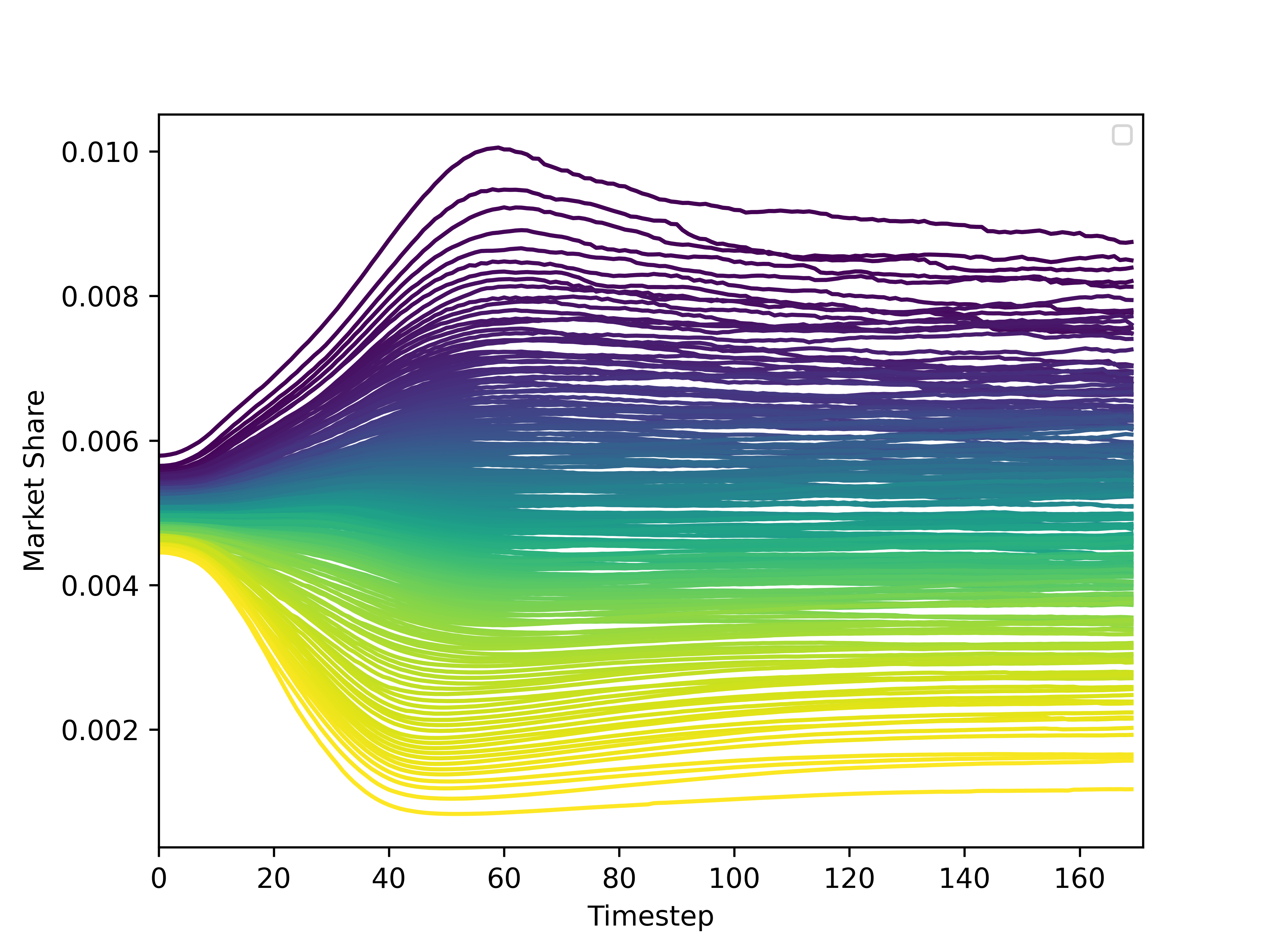
Appendix C: Joint Regression Analysis Heatmap
The following heatmap results are based on the simultaneous sampling of the DSR limit and interest rate, as outlined in Table 3 under ‘Exp 3.’ These results show changes in market concentration, economic growth rate, and labor income share when both policies are varied. In other words, the setup aligns with the joint regression analyses conducted for RQ 1 and RQ 2, with all the parameters other than the financial policy variables being identical to the calibrated parameters in Table 2.
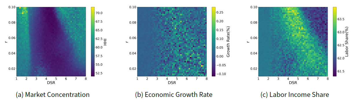
As shown in Figure 9, all three variables exhibit a linear trend with respect to changes in the interest rate, but a nonlinear trend with respect to changes in the DSR limit. Specifically, as the DSR limit increases, market concentration initially decreases and then rises again, whereas the economic growth rate and labor income share show the opposite pattern, first increasing and then declining. Notably, the negative correlation between market concentration and labor income share is prominently illustrated in this figure.
Additionally, the tipping point or inflection point shifts depending on the interest rate; the lower the interest rate, the higher the tipping point for the DSR limit. This indicates a synergistic effect of the two policies. When interest rates are low, a substantial relaxation of DSR regulations tends to benefit small firms. However, when interest rates are high, relaxing DSR regulations can disadvantage small firms by allowing them to dominate the market more easily. Lastly, the negative correlation between market concentration and labor income share, supported by previous studies, is more pronounced in Figure 9a and 9c.
References
ABOAGYE, A., Pyle, D., & Silbey, A. (2014). By the numbers: R&D productivity in the semiconductor industry. Available at: https://www.mckinsey.com/~/media/mckinsey/dotcom/client_service/semiconductors/issue%204%20autumn%202014/pdfs/mosc2014_by_the_numbers_rnd_productivity_in_the_semiconductor_industry.pdf
ADALET, M., Andrews, D., & Millot, V. (2018). The walking dead? Zombie firms and productivity performance in OECD countries. Economic Policy, 33(96), 685–736.
AKCIGIT, U., & Ates, S. T. (2021a). Ten facts on declining business dynamism and lessons from endogenous growth theory. American Economic Journal: Macroeconomics, 13(1), 257–298. [doi:10.1257/mac.20180449]
AKCIGIT, U., & Ates, S. T. (2021b). Ten facts on declining business dynamism and lessons from endogenous growth theory. American Economic Journal: Macroeconomics, 13(1), 257–298. [doi:10.1257/mac.20180449]
ARCAND, J., Berkes, E., & Panizza, U. (2015). Too much finance? Journal of Economic Growth, 20(2), 105–148. [doi:10.1007/s10887-015-9115-2]
ARROW, K. J. (2009). Economic welfare and the allocation of resources for invention. Available at: https://www.nber.org/system/files/chapters/c2144/c2144.pdf
AUDRETSCH, D. B., & Acs, Z. J. (1991). Innovation and size at the firm level. Southern Economic Journal, 57(3), 739–744. [doi:10.2307/1059787]
BANERJEE, R. N., & Hofmann, B. (2018). The rise of zombie firms: Causes and consequences. Available at: https://www.bis.org/publ/qtrpdf/r_qt1809g.htm
BECK, T., Demirgüç-Kunt, A., & Maksimovic, V. (2005). Financial and legal constraints to growth: Does firm size matter? The Journal of Finance, 60(1), 137–177. [doi:10.1111/j.1540-6261.2005.00727.x]
BECK, T., & Levine, R. (2004). Stock markets, banks, and growth: Panel evidence. Journal of Banking and Finance, 28(3), 423–442. [doi:10.1016/s0378-4266(02)00408-9]
BECK, T., Levine, R., & Loayza, N. (2000). Finance and the sources of growth. Journal of Financial Economics, 58(1–2), 261–300. [doi:10.1016/s0304-405x(00)00072-6]
BERNANKE, B., Gertler, M., & Gilchrist, S. (1996). The financial accelerator and the flight to quality. The Review of Economics and Statistics, 78(1), 1–15. [doi:10.2307/2109844]
BLECKER, R. A. (2016). The US economy since the crisis: Slow recovery and secular stagnation. European Journal of Economics and Economic Policies: Intervention, 13(2), 203–214. [doi:10.4337/ejeep.2016.02.05]
BLOOM, N., Jones, C. I., Van Reenen, J., & Webb, M. (2020). Are ideas getting harder to find? American Economic Review, 110(4), 1104–1144. [doi:10.1257/aer.20180338]
CABALLERO, R. J., Hoshi, T., & Kashyap, A. K. (2008). Zombie lending and depressed restructuring in Japan. American Economic Review, 98(5), 1943–1977. [doi:10.1257/aer.98.5.1943]
CARLSTROM, C. T., & Fuerst, T. S. (1997). Agency costs, net worth, and business fluctuations: A computable general equilibrium analysis. The American Economic Review, 87(5), 893–910. [doi:10.26509/frbc-wp-199602]
CECCHETTI, S. G., & Kharroubi, E. (2012). Reassessing the impact of finance on growth. Available at: https://papers.ssrn.com/sol3/Delivery.cfm/SSRN_ID2117753_code456443.pdf?abstractid=2117753&mirid=1
CERDEIRO, D. A., & Ruane, C. (2022). China’s declining business dynamism. International Monetary Fund.
CHEN, S., & Lee, D. (2023). Small and vulnerable: SME productivity in the great productivity slowdown. Journal of Financial Economics, 147(1), 49–74. [doi:10.1016/j.jfineco.2022.09.007]
CLOYNE, J., Ferreira, C., Froemel, M., & Surico, P. (2018). Monetary policy, corporate finance and investment. Available at: https://www.nber.org/system/files/working_papers/w25366/w25366.pdf [doi:10.3386/w25366]
COOLEY, T. F., & Quadrini, V. (2006). Monetary policy and the financial decisions of firms. Economic Theory, 27(1), 243–270. [doi:10.1007/s00199-004-0553-x]
CYNAMON, B. Z., & Fazzari, S. M. (2015). Rising inequality and stagnation in the US economy. European Journal of Economics and Economic Policies: Intervention, 12(2), 170–182. [doi:10.4337/ejeep.2015.02.03]
DAVIS, S. J., & Haltiwanger, J. (2014). Labor market fluidity and economic performance. Available at: Available at: https://ideas.repec.org/p/nbr/nberwo/20479.html [doi:10.3386/w20479]
DOSI, G., Fagiolo, G., Napoletano, M., & Roventini, A. (2013). Income distribution, credit and fiscal policies in an agent-based Keynesian model. Journal of Economic Dynamics and Control, 37(8), 1598–1625. [doi:10.1016/j.jedc.2012.11.008]
DOSI, G., Fagiolo, G., & Roventini, A. (2010). Schumpeter meeting Keynes: A policy-friendly model of endogenous growth and business cycles. Journal of Economic Dynamics and Control, 34(9), 1748–1767. [doi:10.1016/j.jedc.2010.06.018]
FREEMAN, D., Bettendorf, L., van Heuvelen, H., & Meijerink, G. (2021). The contribution of business dynamics to productivity growth in the Netherlands. CPB Netherlands Bureau for Economic Policy Analysis. [doi:10.2139/ssrn.4803858]
GERTLER, M., & Bernanke, B. (1989). Agency costs, net worth, and business fluctuations. The American Economic Review, 79(1), 14–31. [doi:10.3386/w2015]
GORDON, R. J. (2016). The Rise and Fall of American Growth. Berlin: De Gruyter Brill.
GRAVES, S. B., & Langowitz, N. S. (1993). Innovative productivity and returns to scale in the pharmaceutical industry. Strategic Management Journal, 14(8), 593–605. [doi:10.1002/smj.4250140803]
GREENWOOD, J., & Jovanovic, B. (1990). Financial development, growth, and the distribution of income. Journal of Political Economy, 98(5), 1076–1107. [doi:10.1086/261720]
GUERINI, M., & Moneta, A. (2017). A method for agent-based models validation. Journal of Economic Dynamics and Control, 82, 125–141. [doi:10.1016/j.jedc.2017.06.001]
HEIN, E. (2019). Financialisation and tendencies towards stagnation: The role of macroeconomic regime changes in the course of and after the financial and economic crisis 2007-09. Cambridge Journal of Economics, 43(4), 975–999. [doi:10.1093/cje/bez022]
KARAHAN, F., Pugsley, B., & Şahin, A. (2019). Demographic origins of the startup deficit. Available at: https://www.nber.org/system/files/working_papers/w25874/w25874.pdf [doi:10.3386/w25874]
KIM, K. (2018). Diminishing returns to R&D investment on innovation in manufacturing SMEs: Do the technological intensity of industry matter? International Journal of Innovation Management, 22(7), 1850056. [doi:10.1142/s1363919618500561]
KIYOTAKI, N., & Moore, J. (1997). Credit cycles. Journal of Political Economy, 105(2), 211–248. [doi:10.1086/262072]
KRISHNAN, K., Nandy, D. K., & Puri, M. (2014). Does financing spur small business productivity? Evidence from a natural experiment. The Review of Financial Studies, 28(6), 1768–1809. [doi:10.1093/rfs/hhu087]
KROEN, T., Liu, E., Mian, A., & Sufi, A. (2021). Falling rates and rising superstars. Available at: https://www.nber.org/papers/w29368 [doi:10.3386/w29368]
LEVINE, R. (2005). Finance and growth: Theory and evidence. In P. Aghion & S. N. Durlauf (Eds.), Handbook of Economic Growth (pp. 865–934). Amsterdam: North-Holland. [doi:10.1016/s1574-0684(05)01012-9]
LIU, E., Mian, A., & Sufi, A. (2022). Low interest rates, market power, and productivity growth. Econometrica, 90(1), 193–221. [doi:10.3982/ecta17408]
LIU, P., & Chen, S. (2023). The effect of banking deregulation on R&D investment: Evidence from the cross-regional operation of city banks. Journal of Innovation & Knowledge, 8(4), 100451. [doi:10.1016/j.jik.2023.100451]
LUCAS, R. E. (1976). Econometric policy evaluation: A critique. Carnegie-Rochester Conference Series on Public Policy. [doi:10.1016/s0167-2231(76)80003-6]
MADSEN, J. B. (2007). Are there diminishing returns to R&D? Economics Letters, 95(2), 161–166. https://doi.org/10.1016/j.econlet.2006.09.009 [doi:10.1016/j.econlet.2006.09.009]
OTTONELLO, P., & Winberry, T. (2020). Financial heterogeneity and the investment channel of monetary policy. Econometrica, 88(6), 2473–2502. [doi:10.3982/ecta15949]
PALLEY, T. I. (2015). Inequality, the financial crisis and stagnation: Competing stories and why they matter. Available at: https://ideas.repec.org/p/imk/wpaper/151-2015.html
SCHUMPETER, J. A. (1943). Capitalism, Socialism, and Democracy. New York, NY: Harper & Brothers.
SINGH, A. (2004). Multilateral competition policy and economic development. Available at: https://digitallibrary.un.org/record/524232?v=pdf
VAN Stel, A., Lokshin, B., & De Vries, N. (2019). The effect of SME productivity increases on large firm productivity in the EU. Kyklos, 72(2), 332–353. [doi:10.1111/kykl.12198]
VAN Treeck, T. (2015). Inequality, the crisis, and stagnation. European Journal of Economics and Economic Policies: Intervention, 12(2), 158–169. [doi:10.4337/ejeep.2015.02.02]
WOOD, J. D. (2016). The effects of the distribution of mortgage credit on the wage share: Varieties of residential capitalism compared. Comparative European Politics, 15(6), 819–847. [doi:10.1057/s41295-016-0006-5]