Structural Sculpting: Making Inverse Modelling Generate and Deal with Variable Structures

,
and
aDelft University of Technology, Netherlands; bUniversity of Bremen, Germany
Journal of Artificial
Societies and Social Simulation 28 (4) 10![]()
<https://www.jasss.org/28/4/10.html>
DOI: 10.18564/jasss.5830
Received: 21-Nov-2024 Accepted: 13-Oct-2025 Published: 31-Oct-2025
Abstract
When dealing with Agent-Based Models (ABMs), calibration, sensitivity analysis, and robustness testing are often limited to parameter space and seeding, while structural calibration is omitted. However, we know that model structure necessarily also influences model outcome. Omitting structural calibration would thus pose a significant hurdle to robust model-based decision support, policy evaluation, and behavioural insights. Inverse modelling is an explorative modelling approach newly introduced for ABMs, aimed at directly inferring the generative mechanisms underlying observed outcomes by iteratively posing forward problems to match the ABM output with the desired patterns. We propose a method that leverages the inverse method on an ABM's building blocks to calibrate the model for generative insights structurally. We exemplify this through a case study using a solar panel diffusion model with Dutch province-level data, for which we operationalise "structure" through the order and presence or absence of procedures called in the model iteration. Our method shows that it is possible to vary and evaluate model structures automatically via inverse modelling. We find structures that fit each province’s solar panel adoption curve well and others poorly, and that variations, structural or in seed, significantly influence model outcome. We find multiple alternative well-performing model structures that exhibit large deviations concerning order and even the presence of functions. We exemplify how these structures can be made sense of and point directions for further real-life investigations and theory-building, such as the effect of hassle factors or complexity perceptions on adoption rates. With this, we present not an automated replacement of the participatory modelling process but an add-on to systematically reflect on the structure, implementation, and validity of the ABM and the theory utilised.Introduction
In all domains of application, Agent-Based Models (ABMs) display challenges to robust decision support, policy evaluation, and behavioural insights; this could be due to uncertainty concerning parametric settings, the structural assembly of the model, or deterministic chaos due to seeding (Dam et al. 2013), but also behavioural realism (De Vries et al. 2021) or interpretability (Wijermans et al. 2020) and validation (Collins et al. 2024). Much work has been done on calibration and uncertainty quantification. For example, ten Broeke et al. (2016) and Naumann-Woleske et al. (2022) discuss sensible ways to perform sensitivity and robustness analyses. Additionally, Reuillon et al. (2013) provides the cloud platform OpenMOLE for large-scale numerical experiments and model exploration.
However, structurally scrutinising ABMs remains challenging to achieve methodologically (Grimm & Railsback 2012) as conceptual uncertainties are difficult to quantify (Hendricks Franssen et al. 2009), and the ABM body of knowledge currently lacks a methodological approach for assessing structural changes in a generally applicable manner. Experiments to address this problem have been undertaken (cf. Muelder & Filatova 2018; Vu et al. 2023), however, broad systemic structural variation and validation would be a combinatorial problem yielding a vast collection of rules, so from "a single model with no sense of how unique it may be [to] the opposite problem of needing to make sense of a potentially vast collection" (Collins et al. 2024 p. 15) for which there is no general approach or methodology either. In this research, we conjecture that – while an upper bound on possible structural changes exists in principle – the effective upper bound is resource-related and pragmatic rather than theoretical, and we propose a prototype to handle such a combinatorially large search and evaluation process.
In this work, we denote by “structure” the list of rules or function calls that make up one iteration of an agent-based model; this includes the presence or absence of functions as well as their ordering.
While the “forward problem” of an ABM moves from cause to effect, from given initial conditions to an unknown model outcome, the “backward” or “inverted problem” determines the unknown initial conditions that produce a given model outcome. This we call “inverse modelling”, moving from effect to cause. Analytically inverting ABMs, however, is unlikely to be feasible1 and instead, multiple forward problems are iteratively posed. Based on prior differences, the output data are compared to the data to be matched, thereby enabling data-targeted model exploration. Inverse Generative Social Science (iGSS) has recently been proposed as a data-driven methodology for such targeted macro-level pattern matchings for ABMs (Epstein 2023). Applications of iGSS thus far range from opinion dynamics and flocking behaviour (Greig et al. 2023), residential segregation (Gunaratne et al. 2023), irrigation (Miranda et al. 2023), and alcohol use (Vu et al. 2023). The concept itself has been introduced similarly as Pattern-Oriented Modelling (POM) in the work of (Grimm et al. 2005; Grimm & Railsback 2012), or discussed in circles outside of ABM as more generally “inverse simulation” (e.g., Murray-Smith 2000; Hendricks Franssen et al. 2009; Tian 2023; Zhang et al. 2024).
The prototype we propose for a general approach and methodology to generate and assess structural changes leverages the inverse data-driven approach – iteratively posing optimisation problems to minimise the difference between model output and given observation data – to guide the search process through the option space of structural calibration. Thus, the research question that guides these efforts reads: How can inverse modelling be made to deal with and evaluate variable model structures?
This research encompasses several novel elements. The main contribution is methodological, as a general way of automatically generating and evaluating structural alternatives of a modularly set-up NetLogo (Wilensky 1999) model is proposed. Our code is openly available, reasonably fast, uses genetic and machine-learning-based search techniques, and is designed to give the modellers insight into all model evaluations undertaken. We illustrate the potential of our approach by demonstrating the structural exploration of a model to exemplarily match data on Dutch province-level residential solar panel adoption rates. We further present steps for exploratory sense-making after modelling. While our focus is methodological, understanding these dynamics is an important part of accelerating the energy transition, which urgently demands significant changes to the complex energy system and is an important societal goal.
The paper is outlined as follows: The next section will review the literature on existing inverse approaches, ABM validation, and structural ABM modifications. Thirdly, the methodology section will clarify notions used, cover code and data availability, present the case, model, and data, and elaborate on the approach. Fourthly, the analysis will present the results, including an analysis of the structures identified. The discussion will go deeper into the core findings and reflect on the results, focusing on the case, the field, the inverse method, our approach and its limitations. We conclude with an outlook on future work.
Literature Review
In this section, we first review existing inverse approaches with a focus on both model-based optimisation and recent work on inverse modelling, followed by work on validation in ABM and the role that inverse modelling may play. Thirdly, we discuss structural modifications within ABMs and reusable building blocks (RBB). Finally, we position our work within the existing body of literature, integrating it while highlighting its distinct aspects.
Existing inverse approaches and in agent-based modelling
In model-based optimisation contexts, the “forward problem” denotes the problem where the input is given and the system or model output is observed. “Inverse”, by contrast, denotes the process of iteratively guessing and refining the input of a system to match the observed output with given empirical data by minimising a comparison metric.
Various disciplines operationalise the inverse principle to study non-linear problems, be it for external validation using historic temporal data and data gathered from corresponding experiments or gaining “insights about model deficiencies which may not be so obvious from conventional output response comparisons” (Murray-Smith 2000 p. 240).
“Modelling” is a broadly used term in many fields, so the same applies when adding the prefix “inverse”: Hendricks Franssen et al. (2009) praise inverse modelling a “key step” and describe and compare seven methods for equation-based inverse modelling that are – as Carrera et al. (2005) point out, fundamentally identical and, thus, all – influenced by three factors contributing to uncertainty: conceptual, measurement, and parameter uncertainties. On the latter, there is a predominant focus because it is believed that “parameter uncertainty is the most relevant factor” and that “conceptual uncertainties are difficult to be formalised in a rigorous mathematical framework” (all quotes: Hendricks Franssen et al. 2009 p 851). Indeed, in their review, Zhang et al. (2024) outline parameter estimation methods for agricultural modelling and provide a decision tree for selecting the appropriate method based on model type, and Murray-Smith (2000) formalise the problem of and iterative solutions to “inverse simulation” for aerospace engineering and aircraft applications.
As for agent-based simulations, early works on inverse modelling done by Kurahashi et al. (1999) (see also: Kurahashi 2018; Terano 2007) discuss mathematical and conceptual frameworks for inverse simulation, the latter being focused on genetic methods to deal with their large parameter space (which Payette (2024) terms the “curse of possibilities”) and accepting multiple valid solutions. Their discussion of comparing model output with observation centres around and combines the inverse approach with Pattern-Oriented Modelling (POM) as introduced and discussed in the works of Grimm & Railsback (2012) or Grimm et al. (2005). POM means the “multi-criteria design, selection and calibration of models of complex systems” (Grimm & Railsback 2012 p. 302) and is, as such, well separated and complementary to the inverse approach. Being multi-criteria-oriented, POM acknowledges and stresses the multifacetedness or co-occurrence of phenomena in complex, dynamic systems under study.
For inverse modelling for ABMs and, specifically, social simulation, we must list the special issue from March 2023 in the Journal of Artificial Societies and Social Simulation, which includes the works of Epstein (2023), Gunaratne et al. (2023), Greig et al. (2023), Miranda et al. (2023), and Vu et al. (2023) discuss inverse Generative Social Science (iGSS) in various fields of application. iGSS denotes leveraging inverse modelling for generative social science (Epstein 1999). Practically, iGSS resembles symbolic regression (Udrescu & Tegmark 2020), combining model primitives with operators via genetic programming to fit the ABM output to a given set of empirical targets. As such, iGSS forms one approach of utilising the inverse method for agent-based modelling and is suitable for explaining various phenomena by growing them (Epstein 1999, 2023).
In the special issue, shared agreement is expressed that iGSS holds the potential to test many different theories and feed back into social science. However, this conceptually novel approach also encompasses the following teething problems: Epstein (2023) underlines the necessity for “suitable” data (cf. Epstein 2023 p. 6.13), and Greig et al. (2023) and Gunaratne et al. (2023) discuss effective search processes that deal with complexity measures of rules found and difficulties regarding their interpretability concerning overfitting. Their discussion connects to that of Vu et al. (2023), who further raise questions about the comparability of theories found, the lack of reusable building blocks, and the need for a “joint structure-parameter calibration” (cf. Vu et al. 2023 p. 7.3).
We further see the problem caused by the stochasticity inherent to ABMs and the resulting chaos it may cause. In other words, ABMs involve randomness determined by the seed, giving the output not a deterministic but a probabilistic character. Consider the agent task to “select one other agent within your vision radius” to exemplify this chaotic behaviour. Choosing an agent is random, yielding a distribution of outcomes. If vision radius is a parameter, there is now a parametric dependency of this distribution. While Miranda et al. (2023) mention stochastic elements in agent behaviour, they do not delve into the specific implications of deterministic chaos or the role of random seeds. Indeed, the iteratively posed forward problems are based on prior assessments that need to be trusted, e.g. when employing learning algorithms. Thus, the iterative nature of inverse modelling may multiply the challenges inherent to ABMs.
Despite these challenges, the inverse approach is a way to handle a target-oriented model exploration of a large space of options, thus worth considering and exploring. The challenge then presents itself in statistical measures to handle the uncertainty and, as a result, in methods to evaluate and interpret the large amount of data created.
Validation in agent-based modelling
Indeed, a word on validation is necessary. Later in this article, we use the inverse method to assess valid and alternative structures of the ABM. Validation is a key component to an ABM’s credibility, which Collins et al. (2024, p. 1) define as the “the process of determining if a model adequately represents the system under study for the model’s intended purpose (Erdemir et al. 2020; Grimm et al. 2020; Sargent & Balci 2017); this definition could be simplified further as building the right model (Balci 1998)”. In their article, Collins et al. (2024) discuss nine methods for validation, including iGSS, which, in our opinion, extends seamlessly to inverse methods in general: As inverse methods require data to compare the model results to, “the process itself includes a ‘built-in’ validation-support method in the form of the fitness function” (Collins et al. 2024, p. 15). Through this, the modeller can present quantitative results about and statistical properties of the performance of the many simulations undertaken, helping to build credibility. However, as large as the space of possible combinations of primitives may be – posing yet another challenge in itself – no novel behaviours can be expected but only combinations of those specified a priori (Collins et al. 2024, p. 15).
To aid this, automated search pipelines as inverse methods could be equipped with automatic statistical debugging methods such as those of Gore et al. (2017). Their strategy is to perform trace validation, tracing being “periodically collecting data from a simulation during execution” (Gore et al. 2017 p. 1), and statistical analysis ex-post to relate the tracing result to the output. Therefore, they can identify the model characteristics that cause the output. Such methods hint at the potential effectiveness of automated search methods in exploring and analysing an ABM’s structure-parameter space.
This review is not an exhaustive representation of the work done on validation, but focuses on validation through inverse methods. For a literature review-based framework to integrate validation and evaluation, we refer to the work of Augusiak et al. (2014), who aim to assess quality and reality more comprehensively and transparently. For a meta-theoretical framework for inter-model comparison, we refer to the work of Graebner (2018).
Structural modifications
Model structure or architecture, reflecting conceptual assumptions made and uncertainties therein (Hendricks Franssen et al. 2009), is rarely tackled. Indeed, “structure” is a difficult concept to define and, thus, to formalise and calibrate. One distinction between model parameters and structure is drawn in the essay of Payette (2024), who notes that parameters are “scalar” values within a model – such as numeric, logical, enumerated, all together with their bounds and steps, whether they are fixed or free (cf. Payette 2024 p. 607) – while structure involves the arrangement and interaction rules of agents. While parameters can be explored with automated methods as laid out above, structural changes require a deliberate, formal approach. Payette (2024) emphasises this distinction as crucial, as adjusting parameters does not alter the model’s fundamental nature, but changes in structure can significantly impact its behaviour and outcomes. We agree with this and call for thinking structure and parameters together as decisively outcome-influencing model components.
Few works notably investigate structural changes to ABMs: Muelder & Filatova (2018) show how three formalisations of the theory of planned behaviour lead to different outcomes in results, making ABM outcomes more nuanced to interpret beyond parametric uncertainty and chaos. Meanwhile, Jensen & Chappin (2017), Vu et al. (2023) connect the inverse modelling approach to structural model changes, whereas Vu et al. (2023) parameterise their model using three different social theories and discuss the challenges of joint structure-parameter calibration, Jensen & Chappin (2017) lay out a more general way of selecting suitable models to run inverse simulations and discuss four in depth. Thus, with only three or four structures discussed each, these efforts on structural calibration are far behind the work done for parametric model calibration. While a few more authors are moving in this direction, the number of works pales compared to those concerned with parametric calibration, sensitivity, or robustness.
Related to structural modifications to ABMs, the efforts around reusable building blocks (RBBs) must be mentioned and reviewed next. Grimm et al. (2022) define building blocks as “submodels describing processes that are relevant for a broad range of ABM in a certain application domain”, inferring a local generalisability and reusability to them beyond an individual model. Such standardised or reusable building blocks may improve the validity, scrutiny, transparency, and reproducibility of the ABM and its results (Lee et al. 2015), which are crucial for the applicability and use of the ABM in, e.g. policy advice. As discussed above, experiments with building blocks remain scarce because efforts to provide these in a standardised form and repository remain nascent. RBBs have been discussed most recently through Berger et al. (2024), whose repository will be merged with: agentblocks.org/.
We have laid out how “structure” is an ambiguous, open-ended concept. We understand “structure” as the qualitative design, architecture, rules, and organisation of the model, building the frame of reference within which the parameters are embedded and varied. In this research, we operationalise this definition by equating the “(model) structure” with the list of rules or function calls that make up one iteration of an agent-based model. Thus, given a base model, we can create variations, i.e., (model) structures that are alternative candidates to explain the phenomenon studied, potentially revealing
- structural redundancy by discovering unnecessary loops or, on the other hand, quintessential ingredients.
- structural sensitivities or insensitivities which may point to a generalisability of the dynamic studied with regard to case specificity
- equifinalities, i.e. a set of distinct yet result-equivalent structures.
These may yield a richer discussion and scrutinise social theory building beyond parameter calibration. Indeed, consider the case where two distinct structures give the same result. This equifinality would imply that permutation has no effect on the outcome, and thus, the model’s variables would be independent. Investigating whether or not this is indeed the case according to the theory employed in an interdisciplinary setting opens up areas for future investigation, reveals biases, or scrutinises model implementation and may significantly advance theory building.
Embedding and positioning
There is a need for and a lack of structural scrutiny and calibration in ABMs, and a targeted methodology is necessary for navigating the vast space of options. To address this need and fill this gap, we provide a Python wrapper based on PyNetLogo (Jaxa-Rozen & Kwakkel 2018) for modularly written NetLogo models. The wrapper automatically generates and evaluates alternative ABM structures.
This effort connects to existing inverse modelling approaches by applying and extending the inverse approach to model structures. To be precise, it lets learning genetic algorithms create structural variations and evaluate them against real data iteratively. It is, however, distinct from the work of iGSS, which more resembles symbolic regression with primitives combined by operators. In contrast, our approach does not discover new functions but new function call orderings (which we term “structure”) that aim to reproduce a given empirical outcome. Thus, while iGSS explores structural alternatives within a model by combining primitives with operators, our method generates alternative models by reordering calls of existing functions. The two approaches differ in the granularity and scope of their structural units but are similar in ends: generating model-based hypotheses to inform underlying theory.
Furthermore, this effort relates to RBBs. While RBBs aim to standardise common functions or algorithms in ABM research, theoretically equivalent building blocks may differ in formalisation (Muelder & Filatova 2018) and, therefore, result. However, systematically allowing the testing of formally different but theoretically equivalent building blocks in a model structure may scrutinise the building blocks further and allow testing of the robustness of the result with respect not only to the underlying theory but also to the implementation. Our approach is suitable for RBBs and individual lines of code written within a single block using a base alphabet (“primitives” in the iGSS literature).
Thirdly, our approach represents another perspective on inverse modelling and search pipeline to reveal equifinalities rarely explored by modellers, offering a novel perspective on structural aspects and flexibility of ABMs. More specifically, inverse modelling techniques such as iGSS or our approach can significantly advance theoretical understanding and (empirical) validation of ABMs.
Methodology
Glossary
Before continuing into the technicalities, it is worth defining the notions we will use.
- A “structure” is an ordered list forming an iterative rule that makes up one iteration of an agent-based model.
- The notion “run” denotes one single evaluation of a rule over a fixed number of ticks or iterations.
- Such a run can be “dynamic” or, equivalently, “valid” if the output is changing2; in our case, the model output is a curve in the form of a Python list, and a dynamic run would be a run for which the reported values are changing over time.
- A “mutation” is a specific change applied to a structure that produces a new structure: The options for a mutation are to either add a new function to the structure, remove one, or permute two functions. The functions are those of the base model (see Algorithm 1). The range of mutations were restricted, e.g., the maximum length could not exceed that of the base model, i.e. no function used twice, and similar for a sensible minimum length. The space of possible mutations for a structure is called the “mutation space”.
- The terms “fitness” and “error” are used to describe the quality of a run. We are concerned with a minimisation problem, so a high error corresponds to a low fitness and vice versa.
- A “candidate” is, first of all, a candidate model and, as such, an alternative to the base model. In our code, a candidate is a class instance that holds a structure (to be mutated) and a fitness score (to be minimised), which is the comparison value of the model outcome and the data. At the start of the program, a population of candidates is initialised with their structure (or
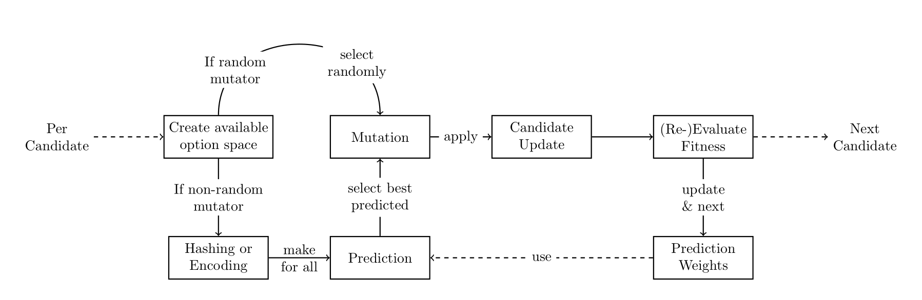
self.actionsin the code) being a random sample of the original model’s functions, see Algorithm 1. The candidates are mutated in each generation, i.e., a mutation is applied to their structure. - This is done by the “mutator”, a higher-level instance that operates on the candidate instances. It evaluates the space of available mutations for a candidate’s current structure, selects one, and applies it to change the candidate’s structure. The mutator can operate randomly or be “learning” (also: “non-random”). In this case, a model is trained on the mutation selected and the fitness outcomes for improved mutation selection. For more details on the internal workings, refer to the Approach Design subsection and Figure 2 therein showing the distinction between random and learning mutators.
Code & model availability
You can find code and model used for this project in a repository on the TU Delft GitLab3. The code is available under Apache 2.0 license or, together with the data generated during the experiments, on the 4TU Repository4, also under Apache 2.0 license.
Case, model, and data
The energy transition in the Netherlands can be said to happen “on the ground” as residential solar panel adoptions have increased drastically (over 2600% from 2012 until 2021) as shown by Zhang et al. (2023 fig. 1). By the end of 2022, a total of 7.2 TWh of renewable energy had been generated with small onshore solar energy projects, reaching the declared goal of at least 7 TWh more than 7 years in advance (Willigenburg et al. 2023). The Netherlands is not famous for its many hours of sunlight or good weather, making its success story a compelling case for understanding the dynamics that drive residential solar panel adoption. Robust results may well inform policy or adoption strategies in other countries. Therefore, while we do not present a fully fleshed-out case study, we exemplify our approach with the real and relevant study of Dutch residential solar panel adoption.
We operationalise this case using the NetLogo model of De Wildt (2014) for residential innovation diffusion and adoption, which was developed for and applied to residential solar panel adoption based on Rogers’ Theory of Innovation Diffusion (Rogers 2014). The model was chosen due to its fitness for the requirements, both case and data-wise, but the code is also modularly written, meaning that the iterative rule of the ABM consists of function calls. The model had to be modified in two instances (see Appendix A) to allow for smooth variation of the building blocks, and the modified version is available in the repository. Figure 1 is an illustrative screenshot of the model.
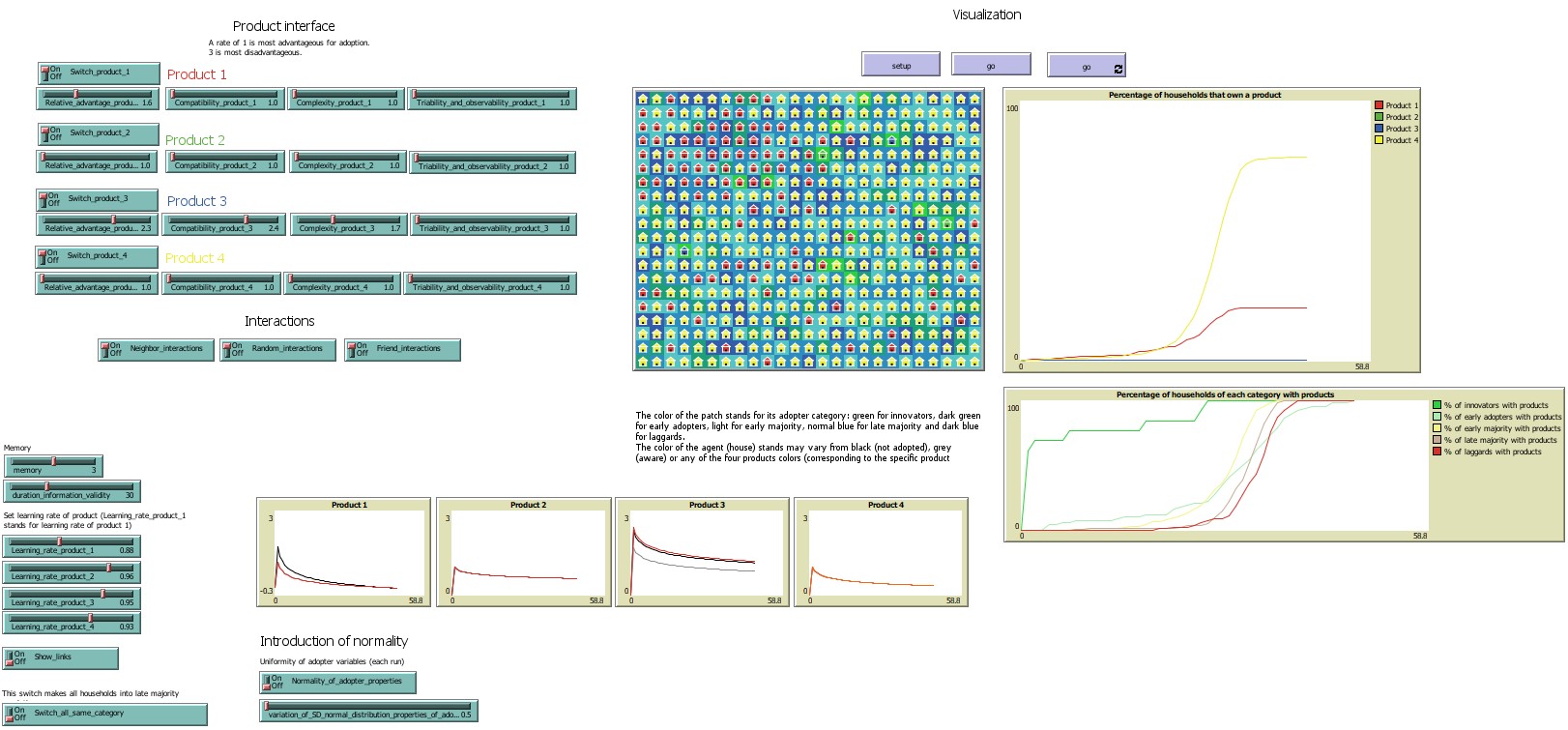
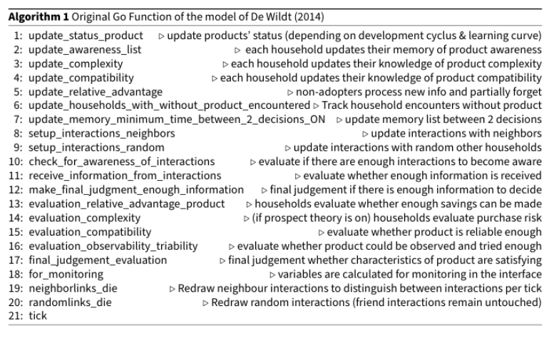
In the model, agents are households starting without a technology, of which there are two competing for adoption: Solar panels and not solar panels as a conscious consumer choice. Through word-of-mouth of neighbours and friends and random interactions, households communicate about the technologies and decide whether to adopt them. Complexity, triability and observability, and compatibility of the technology are set as well as population parameters like memory, learning rate, and, following (Rogers 2014), a division into innovators, early adopters, early majority, late majority, or laggards (De Wildt 2014). The original model’s go function is described in Algorithm 1. Our operationalisation of model “structure” was to equate it with a modified go function. Thus, structurally calibrating the model means generating and testing variations of alternative combinations of this go function by leaving out or permuting the elements of Algorithm 1.
The data are Dutch province-level solar panel adoption rates extracted from the Central Bureau of Statistics on a time frame from 2012 to 2019 (CBS 2019). This time frame is chosen due to, firstly, data availability and data consistency, as after 2019, a new scheme for counting solar panel adoptions has been implemented, and, secondly, to provide a clear, homogeneously produced dataset that is not at risk of being perturbed by the COVID-19 pandemic. The household data are on the province level and from the same time frame (CBS 2024) as the PV adoption data. The PV adoption curves for each province are generated from the residential PV adoption count CBS (2019) and the household data CBS (2024).
Approach design
This subsection elaborates on the Python-based wrapper we built and how it works.
Ta start, the Python wrapper initialises a population of candidates and evaluates each by running it, i.e. running the alternative model and comparing the model output with the target data. Then, for every generation, the mutator instance selects a mutation from the available mutation space, applies it to the candidate-held structure, and re-evaluates the candidate’s fitness. As noted in the glossary, a mutation can add a function to the structure that is not already part of the structure (from the pool of functions, see Algorithm 1), remove one function from the structure, or permute two within the structure. Recall that these options for mutation constitute a candidate’s mutation space. While random mutators select any mutation, learning mutators hold a model instance (such as a random forest regressor) to select mutations. They do so by encoding the mutation space into a machine-interpretable format and predicting the change in fitness, selecting the mutation that is predicted to result in the largest reduction of the error value. The model’s internal prediction weights are updated when the mutator is trained on the results of these runs. To kick off the learning process, learning mutators select a random mutation. This workflow is visualised in Figure 2.
Since the space of possible or allowed structures for the chosen model exceeds \(10^{20}\) model structures5 (not including parameter space), genetic algorithms are chosen to modify the structure one step at a time, either inserting or removing a function or permuting two. The new structure is evaluated using one fixed parameter set over two runs, i.e. only the seed being varied; see Tables 1 and 2 for the parametrisation. While, naturally, two runs do not provide enough data to determine meaningful statistical support for the analysis, this is a simplifying choice targeted at showcasing the ability of the method we propose and at keeping comparability and simplifying the analysis. The code is set up so that multiple parameter sets can be tested over many more runs, too.
In our case, the model output is a curve as a Python list type. We report the number of households that have adopted product 1 at each tick. The resulting curve is compared to the real data using fast dynamic time warping (fastdtw) (Salvador & Chan 2007). Dynamic time-warping techniques are no metric in the mathematical sense but measure the similarity of two curves by aligning their time axes to minimise their cumulative distance (Tavenar 2021). This allows for the comparison of curves differing in length when point-wise methods cannot be employed; indeed, this is the case, see Figure 5 for a side-by-side view of the data and model output. Other time series alignment algorithms are possible, but fastdtw has been chosen for computational speed. The \(x\) axis of the input data is in years, and of the model output in ticks that do not necessarily relate to real time units. Thus, a low or high fastdtw-based error value merely means that the curves are dissimilar or similar.
Lastly, the model output was not pre-processed or modified before being compared with the PV adoption data. This simplifying choice has important consequences: The model will run for a fixed number of iterations and may reach 100% PV adoption. Meanwhile, the Dutch transition has not finished, and we yet lack data beyond today’s adoption levels. This discrepancy makes the model output and data difficult to compare: In a scenario where all available points are matched exactly by the simulation and then continued from there, we would have a perfect fit over the observed range and then more data points from the simulation. Due to the resulting dissimilarity of the curves and the metric chosen, this output would still be associated with a high error value. This underscores the dependency metric chosen. One has three options to avoid this: First, select time series alignment methods that allow partial fit. Second, trim the model output to fit the real data best by, e.g. cutting off at the highest shared \(y\)-value. Third, novel approaches, e.g., a weighted metric, should be developed to treat unobserved future data differently and navigate this difficulty regarding interpretability. Still, each option has other implications and trade-offs, and we will return to these questions in the discussion.
Ex-post analysis and sense-making
The prototype presented serves as a sampler for structural variations of the model. Each iteration is recorded, enabling the analysis of all the runs and thus extracting patterns or individual runs. For a dataset of 20.000 runs, we select an exploratory K.I.D.S. (“Keep it descriptive, stupid!”) approach of Edmonds & Moss (2005) who argue that an “anti-simplistic” way of dealing with the data may reveal more profound insights.
While we circle back to the specifics of the case, “proper” sense-making is out of the scope of this paper and will have to be left for future work. Furthermore, due to the lack of general approaches for sense-making, this work approaches the data analysis through simple, conceptual two-by-two categorisation of fitness quality and plausibility as sketched in Figure 3. For a discussion of the term “plausibility”, we refer to the discussion and leave it as the working definition of “not implausible”. This categorisation is reflected on in the discussion section.
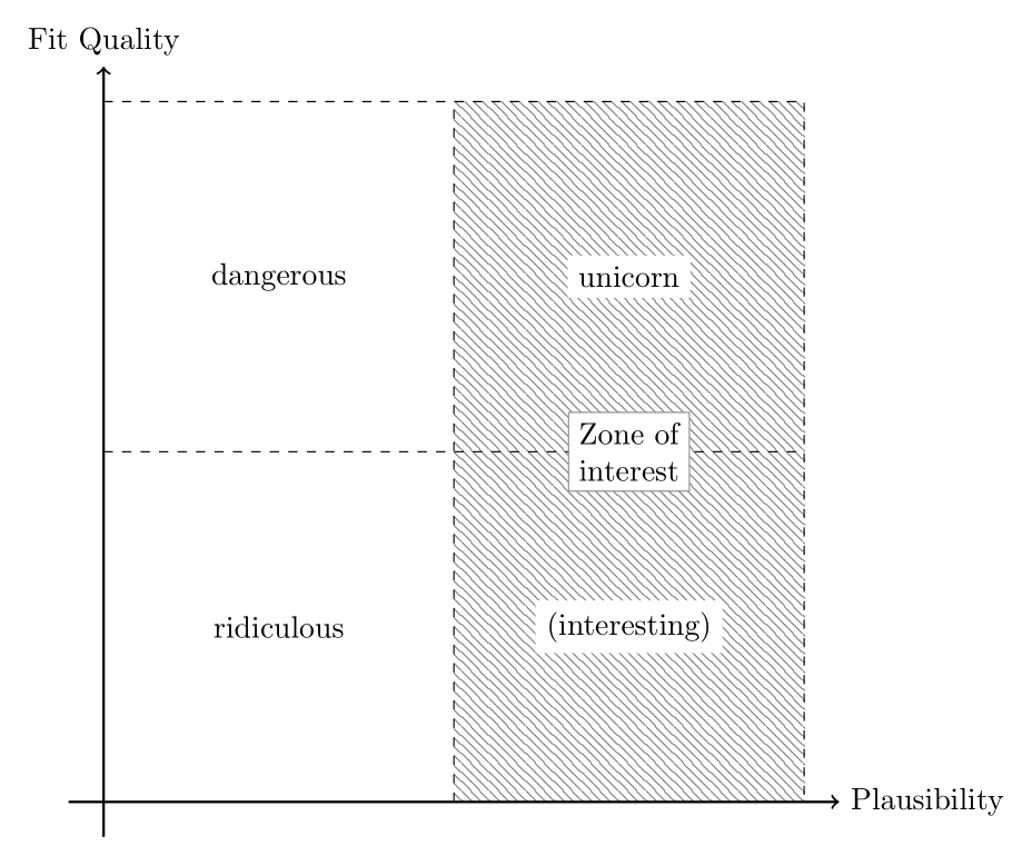
Each structure, “plausible” or not, will have a fitness score on the \(y\)-axis and a conceptual (unknown, difficult to quantify) plausibility value on the \(x\)-axis. We can identify four quadrants:
- Structures with a high fit quality that (unknown to us) are plausible are the unicorn and the main interest for further analysis. If we can find these and make sense of them with the help of domain experts, social scientists, and theorists, we have achieved the ideal of (inverse) generative social science and social simulation.
- Structures with high fit quality but (unknown to us) non-nonsensical are arguably dangerous to feed back into social theory or policy advice. Sorting these out is crucial to avoid bias, (over-)fitting, and other distortions.
- Structures with a poor fit, i.e. a high error, and (unknown to us) not plausible are termed “ridiculous”. The blunt term is chosen to signal that these structures that hold the worst results in both content and fitness are far from being of primary interest for serious investigation or discussion with domain experts.
- Structures, models with a poor fit but, again, unknown to us, high plausibility, are of interest, too. Answering why a model cannot grow a phenomenon it is supposed to grow allows insights into both the implementation and the theory. However, this is of secondary interest due to the importance of the unicorns and is thus put into parentheses.
The analysis will aim to sort the values into these categories. First, an exemplary data analysis will be conducted using a single candidate. Then, our attention goes to the entire dataset of all runs: A subset of the data produced will be considered by sorting out runs and structures that do not produce any dynamics and are thus not of interest. This is a simplifying choice that we take to make sure we perform our analysis only on valid models; we ground this choice in the fact that the model in its original form has been validated by De Wildt (2014), and now select the ones that are “fit-for-purpose” of performing a first, error-based analysis. We later turn towards an integrative pluralistic approach (Mitchell 2009) that takes the stance that multiple models can be correct, although their assumptions conflict.
For the remaining data, the error distribution has a heavy tail with very high error values, making up about 15-20% of the data. For this, pruning will take place using the method described in Appendix B. From a half-violin scatter plot in Figure 9, see that even just the well-behaved, well-performing part of the data remains chaotic, i.e. no clear distribution. We argue that non-standard methods would be necessary to deal with the resulting complexity in the data. We then loop back to structures, identify the unicorn, ridiculous, dangerous, and interesting runs, and visualise them in a dimensionality-reduced way that maintains their spatial distance. We conclude by analysing a set of the most distinct unicorns.
Setup & runs
In total, 20000 different model structures have been evaluated. The computational setup used is the TU Delft’s supercomputer DelftBlue (DHPC 2024). The parameter set used for all runs can be found in Table 1 for the products and Table 2 for the agent population.
| Category | Product 1 | Product 2 |
|---|---|---|
Switch |
True | True |
Learning_rate |
0.88 | 0.96 |
Relative_advantage |
1.6 | 1.0 |
Compatibility |
1.0 | 1.0 |
Complexity |
1.0 | 1.0 |
Triability_and_observability |
1.0 | 1.0 |
The parameters of Table 1 represent two technologies competing for adoption, solar panels versus not adopting solar panels. Both products are set equally for compatibility, complexity, and trialability and observability, making them similarly viable, user-friendly, and observable within the social system. The differences in learning rate and relative advantage between the two products highlight the assumed adoption dynamics. Solar panels (Product 1) have a lower learning rate to indicate a need for adaptation. In comparison, the status quo’s higher learning rate reflects minimal learning as users are already familiar with conventional energy sources. The relative advantage of solar panels showcases perceived benefits like cost savings and environmental impact, whereas the status quo indicates no additional benefits beyond familiarity.
| Parameter | Value |
|---|---|
Random_interactions |
True |
Friend_interactions |
True |
Neighbor_interactions |
True |
Normality_of_adopter_properties |
False |
Memory |
3 |
Variation_of_SD_normal_distribution_properties_of_adopters |
0.5 |
Switch_all_same_category |
False |
Duration_information_validity |
30 |
Analysis
With no general approach or methodology for analysing structural variation, we have conducted an exploratory analysis of the data created. Our exploratory analysis is split up into two parts: first, an analysis of one single candidate over time, which will show key properties of the data, and then for the whole dataset that will follow the same lines in more depth. We have selected this approach to inspire other researchers approaching such kinds of data sets. Thus, we will investigate the error distributions using plots and, more informatively, statistical tests.
Exemplary analysis of one single run
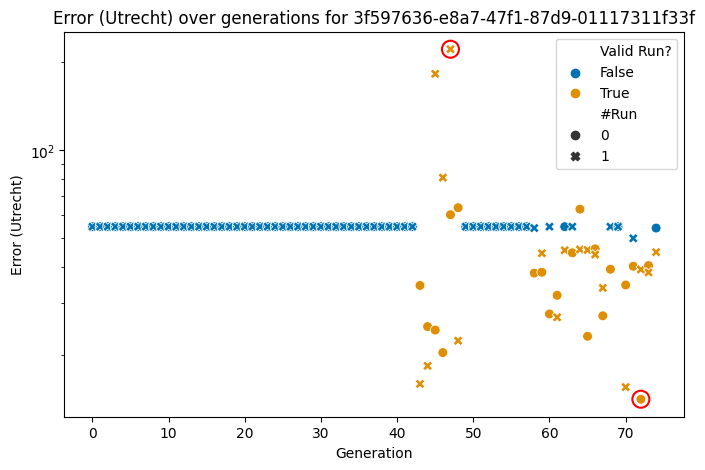
Candidate 3f597636-e8a7-47f1-87d9-01117311f33f was chosen because out of its 150 runs (one candidate being mutated throughout 75 generations with two runs per structure each), it produced 37 valid runs, which is a comparatively high value.
We compare its output against the data of the Dutch province Utrecht and visualise the errors over time in Figure 4 for two runs per structure; i.e. same setting but letting the seed vary. Note that the figure has a log-scale on the \(y\) axis to give more detail to the lower values and less emphasis to the higher values. Orange markers indicate “valid” runs, i.e. runs that produced a dynamic, and blue markers show invalid runs. Each structure is evaluated twice, and the run number is indicated via the marker’s shape.
We see that most of the 150 runs did not produce a dynamic (indicated by blue markers), which may be due to NetLogo errors or simply no dynamics. Those that create a dynamic (orange markers) can perform better or worse than the flat line that invalid runs return. Interestingly, 37 runs produce a dynamic, meaning that at least one structure once did and once did not produce a dynamic. This would suggest that for at least one structure, it was dependent on the seed whether or not a dynamic was produced.
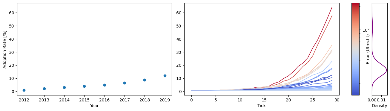
Next, we aggregate the error values, i.e. drop the generation values and focus on the error value distribution of the valid runs (i.e. the distribution of the \(y\)-values of the orange markers of Figure 4) as the invalid runs distort the data and hinder further analysis. Contrasted to the Utrecht data (on the left), the right of Figure 5 displays the model output curves that underlie the error values of the markers of Figure 4. The error distribution shows the error distribution and is based on a symmetric kernel density estimate. We see that even after sorting out the invalid runs, the distribution is still stretched by runs that produce a dynamic but with high error values.
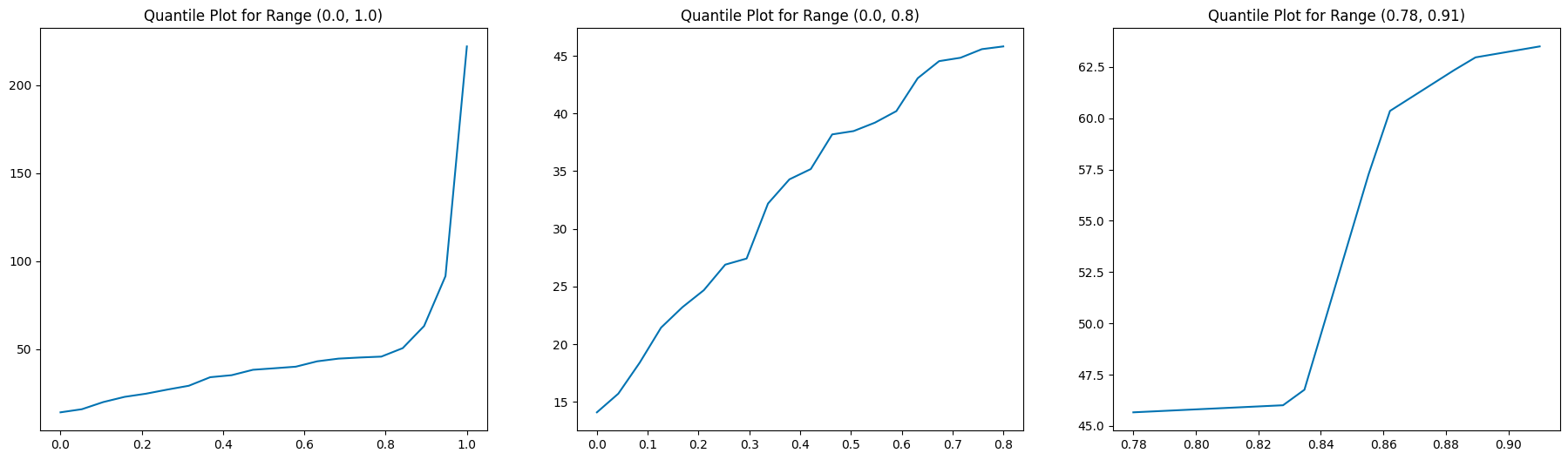
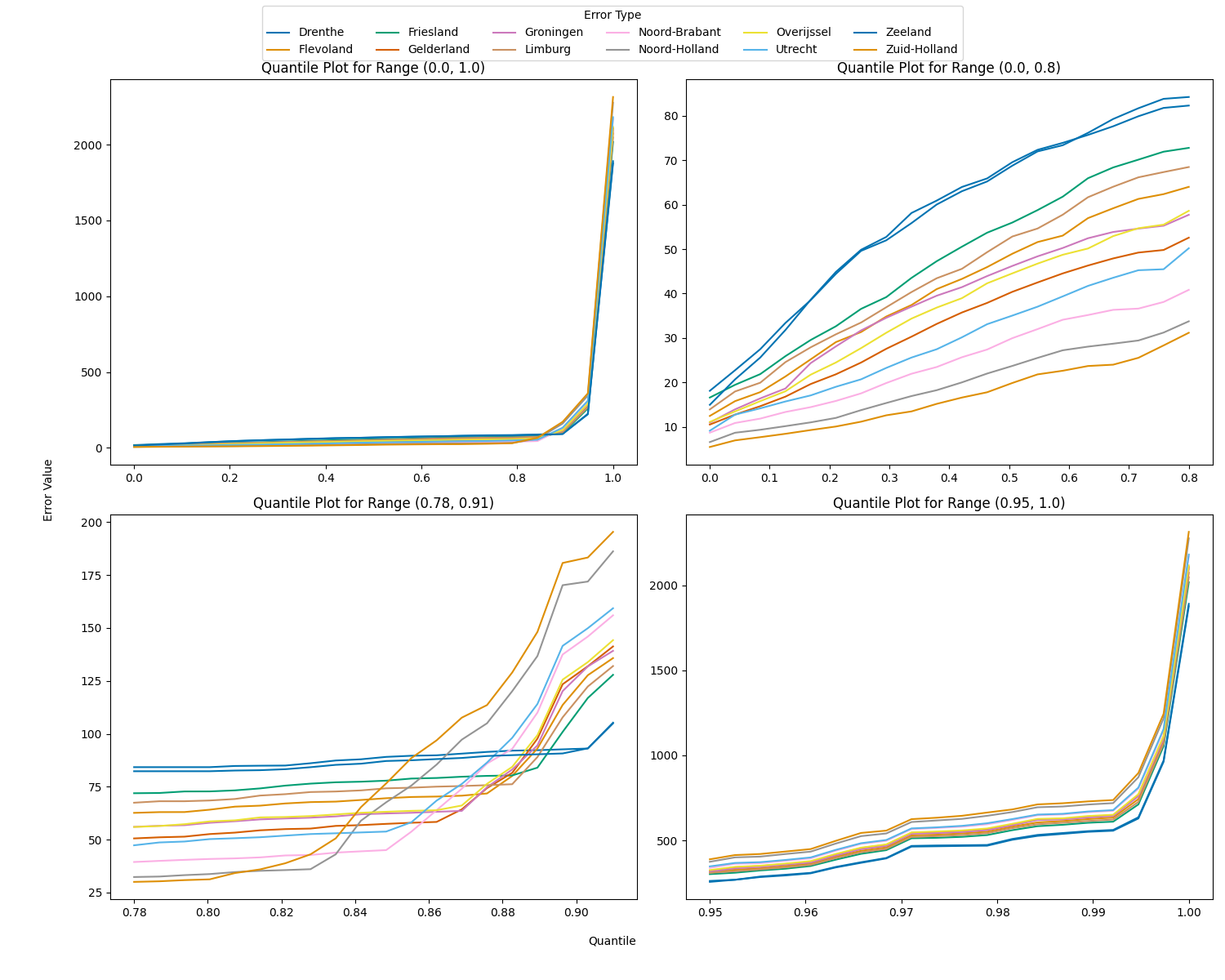
Indeed, these distribution outliers are worth investigating. For this, we visualise the quantile-error relation in Figure 6 for the quantile ranges \([0.0,1.0]\), \([0.0,0.8]\), and, zooming in on the interesting part, \([0.78,.0.91]\) on the \(x\) axis, and the corresponding error cut-off on the \(y\) axis. We can see how the errors are in an exponential relationship to the quantile. For our single candidate, i.e. a family of structures, and in the case of Utrecht, the error value as a function of the quantile “takes off” just above 0.8. We select the “well-behaved” subset using the pruning method described in Appendix B to continue the analysis.
Comparing these three datasets created using descriptive statistics, we get a breakdown of how the data is structured. An overview is given in Table 3 and is now elaborated on.
| Type | Sample | Mean | Med | MAD | Std | Var | Min | Max | Range |
|---|---|---|---|---|---|---|---|---|---|
| Error (all) | 150 | 52.6 | 54.9 | 0.0 | 20.4 | 4.2 × 10² | 14.1 | 221.9 | 207.8 |
| Error (only valid) | 37 | 46.0 | 38.3 | 7.7 | 40.8 | 1.7 × 10³ | 14.1 | 221.9 | 207.8 |
| Error (well-behaved) | 30 | 32.8 | 34.6 | 9.5 | 10.3 | 1.1 × 10² | 14.1 | 45.9 | 31.8 |
| Type | Skew | Kurt | IQR | CV | 10th %ile | 90th %ile | Jarque-Bera |
|---|---|---|---|---|---|---|---|
| Error (all) | 5.3 | 40.6 | 0.0 | 0.4 | 34.6 | 54.9 | 1.1 × 10⁴ |
| Error (only valid) | 3.3 | 10.5 | 18.7 | 0.9 | 19.5 | 63.2 | 2.4 × 10² |
| Error (well-behaved) | −0.3 | −1.2 | 15.9 | 0.3 | 18.1 | 45.0 | 2.4 |
Naturally, the sample size decreases as we select a subset and a subset of that subset. Similarly, we select better and better-rated values and mean and median shrink. It is noteworthy how the standard deviation first increases and then decreases. A high standard deviation combined with a low median indicates that while the bulk of the data is centred around a lower value, extreme outliers increase variability. This is strengthened through a median absolute deviation (MAD) of zero at first and then showing more dispersion of the data.
As we sort out invalid and poorly performing runs, variance increases and decreases afterwards. The invalid runs comprise a large portion of the initial distribution, giving outliers less relative weight. Focusing on the well-behaved quantile, i.e. the top 83%, naturally reduces variance.
Similarly, both skew (asymmetry) and kurtosis (tailedness) values shrink and even turn positive to negative in the last step as the outliers are cut off, leaving the distribution less dominated by its tail.
In the first step, the inter-quantile range (IQR) value is zero, which can be considered extreme, meaning that the centre data is tightly clustered, as we have observed in the amounts of non-valid runs. Only the values of the 10th and 90th percentiles show variation. The 10th and 90th percentile values are the error values where the 10th and 90th percentiles begin, respectively.
Lastly, the Jarque-Bera value, testing for a normal distribution, decreases by an order of \(10^2\) each step, which marks a significant reduction. A value of 2.4 suggests that the distribution is not significantly different from normality. However, a sample size of 30 makes us cautious to assume this generally, and we will come back to this when analysing the entire dataset.
From this exemplary analysis, we learn that it is likely that a data analysis purely based on error values should rely on non-standard techniques equipped to handle non-linearity and non-normality.
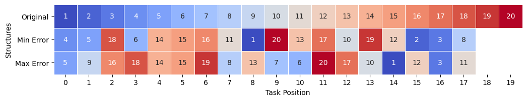
Lastly, we selected two candidates that generated the minimum and maximum error of all the valid runs and compared them to the original highlighted in Figure 4. The heat map Figure 7 visualises this, translating numeric values of placement into a colour gradient and providing an intuitive representation of similarity: The harmonious colour progression in the structure shows alignment with the original, while disruptions in the gradient show deviations. This method facilitates easier detection and interpretation of differences between structures by emphasising visual patterns rather than numerical values. Table 3 presents the tabular overview of what functions the individual digits refer to.
Analysis of all runs conducted
Of the 20.000 runs, 444 produced a changing curve, while all others remained flat. This suggests that most structures tested produce internal NetLogo errors or compile but do not work. We move forward using only the 444 structures that created a dynamic. These remaining, valid structures are evaluated against the data of each province. Table 4 provides a comprehensive overview of the resulting error distribution and will now be discussed.
| Province | Sample | Mean | Med | MAD | Std | Var | Min | Max | Range | |
|---|---|---|---|---|---|---|---|---|---|---|
| Drenthe | 444 | 89.3 | 68.4 | 15.9 | 129.3 | 1.7 × 10⁴ | 18.1 | 1.9 × 10³ | 1.9 × 10³ | |
| Flevoland | 444 | 80.3 | 48.3 | 14.5 | 151.4 | 2.3 × 10⁴ | 12.5 | 2.1 × 10³ | 2.1 × 10³ | |
| Friesland | 444 | 84.4 | 55.8 | 17.0 | 145.0 | 2.1 × 10⁴ | 16.6 | 2.0 × 10³ | 2.0 × 10³ | |
| Gelderland | 444 | 74.5 | 40.2 | 12.4 | 156.7 | 2.5 × 10⁴ | 10.5 | 2.1 × 10³ | 2.1 × 10³ | |
| Groningen | 444 | 78.6 | 45.6 | 11.2 | 154.3 | 2.4 × 10⁴ | 10.9 | 2.1 × 10³ | 2.1 × 10³ | |
| Limburg | 444 | 82.3 | 52.0 | 16.1 | 148.3 | 2.2 × 10⁴ | 13.9 | 2.0 × 10³ | 2.0 × 10³ | |
| Noord-Brabant | 444 | 69.8 | 29.7 | 10.4 | 165.0 | 2.7 × 10⁴ | 8.7 | 2.2 × 10³ | 2.2 × 10³ | |
| Noord-Holland | 444 | 70.9 | 23.6 | 8.8 | 178.1 | 3.2 × 10⁴ | 6.6 | 2.3 × 10³ | 2.3 × 10³ | |
| Overijssel | 444 | 78.1 | 44.4 | 13.2 | 157.0 | 2.5 × 10⁴ | 11.1 | 2.1 × 10³ | 2.1 × 10³ | |
| Utrecht | 444 | 74.6 | 34.9 | 12.6 | 165.3 | 2.7 × 10⁴ | 9.1 | 2.2 × 10³ | 2.2 × 10³ | |
| Zeeland | 444 | 89.2 | 69.4 | 13.9 | 130.5 | 1.7 × 10⁴ | 15.0 | 1.9 × 10³ | 1.9 × 10³ | |
| Zuid-Holland | 444 | 70.7 | 19.7 | 8.5 | 183.5 | 3.4 × 10⁴ | 5.5 | 2.3 × 10³ | 2.3 × 10³ | |
| Province | Skew | Kurt | IQR | CV | 10th %ile | 90th %ile | Jarque–Bera | |||
|---|---|---|---|---|---|---|---|---|---|---|
| Drenthe | 8.0 | 89.8 | 34.2 | 1.5 | 29.7 | 92.9 | 1.5 × 10⁵ | |||
| Flevoland | 7.3 | 75.0 | 31.2 | 1.9 | 18.7 | 123.1 | 1.1 × 10⁵ | |||
| Friesland | 7.4 | 78.7 | 35.2 | 1.7 | 22.5 | 114.7 | 1.2 × 10⁵ | |||
| Gelderland | 7.1 | 71.3 | 25.5 | 2.1 | 15.1 | 128.3 | 9.8 × 10⁴ | |||
| Groningen | 7.2 | 73.2 | 24.0 | 2.0 | 17.3 | 126.5 | 1.0 × 10⁵ | |||
| Limburg | 7.4 | 76.9 | 33.9 | 1.8 | 20.8 | 120.0 | 1.1 × 10⁵ | |||
| Noord-Brabant | 6.8 | 66.5 | 20.4 | 2.4 | 12.6 | 142.2 | 8.5 × 10⁴ | |||
| Noord-Holland | 6.4 | 59.9 | 17.2 | 2.5 | 9.5 | 170.8 | 6.9 × 10⁴ | |||
| Overijssel | 7.1 | 71.5 | 27.9 | 2.0 | 16.4 | 134.1 | 9.8 × 10⁴ | |||
| Utrecht | 6.8 | 66.6 | 24.8 | 2.2 | 15.1 | 146.8 | 8.6 × 10⁴ | |||
| Zeeland | 8.0 | 89.2 | 31.9 | 1.5 | 26.7 | 91.0 | 1.5 × 10⁵ | |||
| Zuid-Holland | 6.3 | 57.2 | 16.6 | 2.6 | 8.0 | 182.0 | 6.4 × 10⁴ | |||
Drenthe and Zeeland have the highest mean values, and Noord-Brabant, Zuid-Holland and Noord-Holland have the lowest. A high standard deviation combined with a low median (like Zuid-Holland, with a median of 19.7 but a standard deviation of 183.5 and median absolute deviation (MAD) of 8.5) indicates that while the bulk of the data is tightly clustered around a lower value, extreme outliers increase variability.
Meanwhile, as seen in Noord-Holland and Zuid-Holland, high variance values suggest that outliers in these provinces are more spread out and heterogeneous, while the low MAD value hints at strong clustering.
All provinces show positive skewness, indicating a right-skewed distribution with outliers or high-value data points. Meanwhile, all provinces show high kurtosis, suggesting the presence of extreme values or outliers, resulting in heavy tails. Drenthe and Zeeland stand out with high kurtosis values, indicating an especially heavy tail. This combination of high skewness and high kurtosis suggests that these distributions are asymmetric and dominated by outliers. It indicates that the outliers are primarily on the upper end, significantly impacting the overall distribution.
All provinces have enormous ranges, showing a significant spread between the smallest and largest error values. Meanwhile, the IQR values are consistently much smaller (by an order of two) than the range, showing that the middle 50% of the data is very tightly clustered. This means the overall variability in the data is primarily driven by outliers, not by general spread within the bulk of the data. Provinces like Noord-Holland and Zuid-Holland show large ranges like all other provinces, but particularly small IQRs, indicating that a few high outliers heavily skew their data.
The 10th and 90th percentile values show significant variation across provinces, but most provinces display widespread in the central 80% of the data. The percentile values confirm the variability seen in other measures.
The Jarque-Bera test returns extremely high values across all provinces, suggesting that the data significantly deviates from a normal distribution, congruent with earlier insights about skewness and kurtosis. Non-normality complicates the analysis, but the test is known to be overly sensitive when dealing with large datasets.
In summary, the data across all provinces is characterised by significant skewness, high kurtosis, and substantial variability driven by outliers, indicating heavy-tailed, asymmetric, and non-normal distributions. This is confirmed when looking at the relationship between quantile value and corresponding error value cut-off as visualised for various quantile ranges in Figure 8: Not only do the error values rise sharply in the worst-performing parts of the data, but also does this rise occur at different points on the \(x\)-axis. As per the analysis above, these outliers heavily obstruct the data analysis. Thus, we identify these province-specific points of interest, after which the data only has outliers using the pruning method explained in detail in Appendix B. Table 5 presents a statistical overview of the newly generated subset.
| Province | Sample | Mean | Med | MAD | Std | Var | Min | Max | Range | |
|---|---|---|---|---|---|---|---|---|---|---|
| Drenthe | 342 | 56.9 | 60.2 | 14.1 | 19.1 | 365.3 | 18.1 | 84.1 | 65.9 | |
| Flevoland | 331 | 39.2 | 40.5 | 12.3 | 14.8 | 220.1 | 12.5 | 62.2 | 49.8 | |
| Friesland | 335 | 45.8 | 47.1 | 14.6 | 16.9 | 284.3 | 16.6 | 71.8 | 55.2 | |
| Gelderland | 326 | 31.4 | 32.5 | 11.2 | 12.2 | 148.3 | 10.5 | 49.7 | 39.2 | |
| Groningen | 321 | 36.3 | 38.9 | 10.8 | 13.4 | 178.4 | 10.9 | 55.0 | 44.0 | |
| Limburg | 332 | 42.3 | 43.2 | 13.2 | 15.8 | 248.7 | 13.9 | 67.2 | 53.2 | |
| Noord-Brabant | 296 | 22.1 | 21.6 | 7.5 | 8.4 | 69.8 | 8.7 | 36.3 | 27.6 | |
| Noord-Holland | 285 | 17.0 | 16.4 | 5.9 | 6.5 | 42.6 | 6.6 | 28.6 | 22.1 | |
| Overijssel | 328 | 34.8 | 36.2 | 11.8 | 13.6 | 184.1 | 11.1 | 55.4 | 44.3 | |
| Utrecht | 322 | 27.5 | 26.4 | 9.8 | 10.7 | 113.6 | 9.1 | 45.4 | 36.3 | |
| Zeeland | 343 | 56.7 | 61.3 | 13.5 | 19.4 | 377.0 | 15.0 | 82.3 | 67.4 | |
| Zuid-Holland | 277 | 13.7 | 12.8 | 4.3 | 5.3 | 28.5 | 5.5 | 23.7 | 18.2 | |
| Province | Skew | Kurt | IQR | CV | 10th %ile | 90th %ile | Jarque–Bera | |||
|---|---|---|---|---|---|---|---|---|---|---|
| Drenthe | -0.4 | -1.0 | 29.7 | 0.3 | 27.3 | 80.4 | 23.8 | |||
| Flevoland | -0.1 | -1.2 | 25.3 | 0.4 | 17.2 | 59.0 | 21.9 | |||
| Friesland | -0.1 | -1.3 | 28.4 | 0.4 | 21.3 | 68.7 | 21.9 | |||
| Gelderland | -0.1 | -1.3 | 22.0 | 0.4 | 14.4 | 47.4 | 21.6 | |||
| Groningen | -0.3 | -1.2 | 22.5 | 0.4 | 16.1 | 53.2 | 24.0 | |||
| Limburg | -0.1 | -1.2 | 26.0 | 0.4 | 19.2 | 64.0 | 21.9 | |||
| Noord-Brabant | 0.2 | -1.3 | 15.3 | 0.4 | 11.4 | 34.6 | 21.9 | |||
| Noord-Holland | 0.2 | -1.3 | 11.9 | 0.4 | 9.1 | 26.9 | 21.7 | |||
| Overijssel | -0.2 | -1.3 | 24.3 | 0.4 | 15.1 | 52.3 | 24.9 | |||
| Utrecht | 0.1 | -1.3 | 19.2 | 0.4 | 13.8 | 42.7 | 24.9 | |||
| Zeeland | -0.6 | -0.9 | 30.6 | 0.3 | 25.1 | 79.0 | 21.9 | |||
| Zuid-Holland | 0.3 | -1.2 | 9.1 | 0.4 | 7.3 | 22.1 | 21.7 | |||
We observe that the means are generally lower, as expected, although not as much as a reduction to the (by now) lowest 1-2% of the total dataset would make one think. Median and mean are, again, very close to each other, while standard deviation decreased by an order of 10 and, consequently, so does variance by an order of \(10^2\). Median absolute deviation halves by a factor of 2 in the case of Zuid-Holland (4.3 from 8.5 before) and hardly changes in the case of Drenthe (14.1 from 15.9 before). The minimum remains the same, and the maximum shrinks together with the range as we expected.
The now negative skewness occurs because we have truncated the right tail (which pulls the distribution toward high values), leaving the distribution dominated by the lower end. This, too, is as expected.
Kurtosis is also negative and decreased by an order of 10. This suggests that without the influence of extreme values, the low quantiles are more “uniformly distributed”, i.e. data shows fewer extreme deviations and is flatter than a normal distribution.
The 10th and 90th percentiles decrease as one would expect. However, with significant inter-provincial variance: In Drenthe, the 10th percentile is 27.3, and the 90th percentile is 80.4, indicating wide variability across the distribution (29.7 and 92.9 before, respectively). In contrast, Zuid-Holland has a much tighter percentile range (7.3 to 22.1), reflecting the lower variability in other metrics (8.0 and 182.0 before, respectively).
The result of the Jarque-Bera test has decreased from an order of \(10^5\) to an order of \(10^1\), which marks a very significant decrease. Still, all provinces largely differ from a normal distribution. This is backed by further reducing this subset’s size as the Jarque-Bera test is now more reliable, and the prior test might have been overly sensitive due to the extreme skewness and kurtosis driven by outliers, which are now removed.
The dramatic reduction in skewness and kurtosis suggests that parametric tests, previously unsuitable for the whole dataset, could be more appropriate for the subset. Removing extreme outliers has made the subset distribution more stable and potentially easier to model with standard statistical techniques. At the same time, the persistence of high Jarque-Bera values, even in the small subset, refutes the assumption of normality. We will discuss this property further in the discussion.
The hypothesised, persisting non-normality is confirmed when plotting the error values of this well-behaved subset, see Figure 9: On the \(x\)-axis, we have the 12 provinces, and on the \(y\)-axis the error value of the structures within the subset. For each province, we have two subplots: a violin plot showing the aggregated data distribution and a scatter plot showing the scatter of the actual structures and their error values, together with a boxplot with median (the line) and mean (the dot marker).
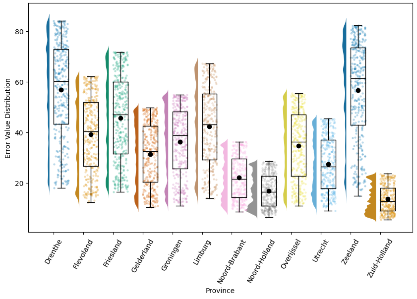
Overall, the data does not resemble a normal distribution, and it would be a similar stretch to call it uniformly distributed. As could be read from the descriptive analysis, the distributions of Noord-Holland, Zuid-Holland, and maybe Noord-Brabant are very low on the \(y\)-axis compared to other provinces and quite dense. Meanwhile, Drenthe, Zeeland, and maybe Friesland have, by comparison, long distributions with higher values overall. Overall, the model had trouble fitting Drenthe, Zeeland, and maybe Limburg, but it was comparably more straightforward to fit Noord-Holland, Zuid-Holland, and maybe Noord-Brabant.
Looping back to structures
When considering Figure 8 and the subsets, it is unclear which structure is in which part, i.e. whether the same structure made the cut for all provinces, for none, or merely for some. Merging the subset with the original 444 and filling in NaN where the structure did not make the cut gives a distribution as shown in Figure 10: The figure visualises the probability of a structure not to fit \(x\) amount of provinces, i.e. how many fits a valid structure can fail. Thus, the height of the bar denotes the probability in total, and the stacked colours indicate the contribution of each province.
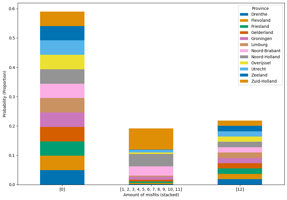
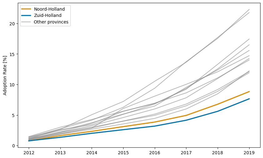
We see a high chance of almost 60% for \(x = 0\), meaning a structure’s fit quality would be good enough to make the cut for all provinces. For \(x=12\), meaning that a structure would not fit any province well enough, we observe a probability of about 25%. In both cases, trivially, each province’s contribution is equal. For all partial fits, the chances are slim, around less than 5% individually. Stacking them up, however, reveals that Zuid-Holland and Noord-Holland, in particular, have a comparably large share of partial misfits. This is particularly interesting in the face of the results of Figure 9, where these two provinces have dense, compact, and overall low error value distributions. Their adoption curves are visualised and distinguished from all other curves in Figure 11 where the \(x\) axis is the year and the \(y\) axis is the adoption rate in percentage. It shows that these two provinces have the overall lowest and slowest rates of adoption. When we compare this to what we know about the data from Figure 5 where we have seen that the majority of model output curves end at a relatively low point on the \(y\) axis, this could be a possible explanation as to why these two provinces yield overall good fits. This has various implications for data preparation for inverse modelling, which will be discussed further in the next section.
The distribution of Figure 10 distinguishes three categories. This, in turn, allows us to sort the 20.000 runs into four categories as our fitness-plausibility framework (cf. Figure 3) requires: Firstly, structures that only had flawed runs, i.e. runs that do produce a dynamic but are evaluated with high error values, can be considered not the primary interest but interesting for second-order data analysis. The second group holds structures that fit every province’s curve well enough to make the cut. These perfect-fit structures are equated with the “unicorn” category. Thirdly, consider structures that only make a partial fit. We equate them with the “dangerous” category as they only give an unreliable or partial fit. Lastly, most runs that produce no dynamic are labelled as “ridiculous”; these are the ones we sorted out first.
Note that the choice between categories 2 and 3 is highly questionable! Equating high plausibility with the attribute of fitting every curve is a choice made for being able to distinguish and move forward. Aiming “One structure to fit them all” has wide implications regarding overfitting, model-theory connection, and interpretability. In other words: Are general, good-at-everything structures desirable or is one best structure per data point preferred? We postpone further discussion of this until the next section.
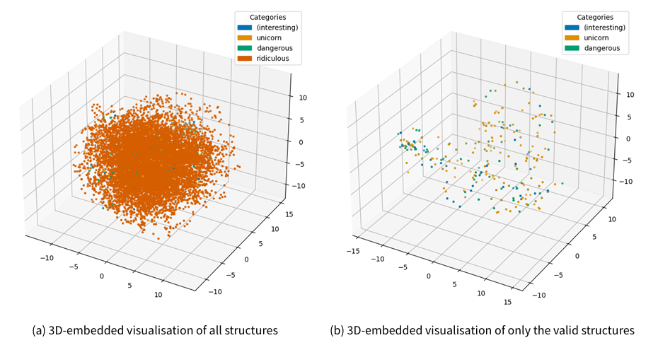
This distinction, however, allows for a visualisation based on the categories of Figure 3. Using the Damerau-Levenshtein distance, we measure the pairwise distances between the individual structures and obtain a distance matrix of size 20.000 by 20.000. The Damerau-Levenshtein distance is the minimum number of permutations, insertions, and deletions necessary to get from one element to the other. This is a convenient choice as this is the way the mutator changes one candidate in one generational update. Compressing and embedding this into a 3D space that takes 30 neighbours into account to represent the pairwise distances as accurately as possible, we get a visualisation as in Figure 12.
Both subfigures are three-dimensional plots where each marker represents one structure. Figure 12a holds all structures, Figure 12b only the structures of the category “unicorn”, “interesting”, and “dangerous”. We see, firstly, that the “ridiculous” category makes up the majority of points. Secondly, no clear, well-separated cluster is visible for either category: Runs of all dynamic structures are well spread out over space, and no clear clusters can be made out, either together or by colour. Producing a dynamic and yet being structurally distinct to a large degree would indicate that, firstly, it is easy to break a model through only changes, and, secondly, it is possible to find functioning models many changes away.
Lastly, recall that at least one structure produced one valid and one invalid output. This raises questions about how much the structures overlap through these categories. The distinction we made allows us to create a Sankey diagram that shows whether one structure is solely in one category or whether there is a significant deviation and, thus, a large overlap between the categories. This is visualised in Figure 13.
Note that the figure is normalised, meaning that the bars for the categories have been scaled to be the same size. This choice has been made to aid visualisation since. Otherwise, category “ridiculous”, 19556 out of 20000, runs would dominate the visualisation.
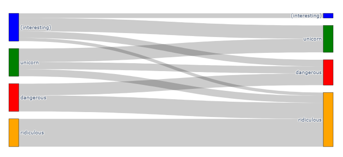
The Sankey diagram shows that many structures remain in the same category for both runs. However, significant exchange between them suggests only partial stability in classification: Yet, the overlap from category “ridiculous” into categories “unicorn”, “interesting”, and “dangerous” appears as tiny relative to the share of runs that are shared between the latter three categories. This indicates that a considerable set of structures had half of their runs producing a dynamic, and the other half did not. This could be taken as an indicator that our assignment into these categories requires improvement for future work. An alternative interpretation would be that seed and stochasticity are vital to consider, e.g. by picking individual structures that yield very different outcomes and investigating what this is due to.
Note that this result comes from only two runs on the same structure. It raises questions about the seed-robustness of the model, i.e. whether the same structure and parameter set for merely two different initial conditions should have such an effect, once with and once without dynamic, on the model output.
Structural analysis
Finally, for our structural analysis, we select the largest subset of all runs that match everything well with maximum pairwise distance. Again, distance is the Damerau-Levenshtein distance.
From Figure 14, we can gather a set of observations. Note that the pattern at the end of [19, 20] was fixed ex-ante. These clean-up functions in the original model were excluded from the variation to reduce the search space.
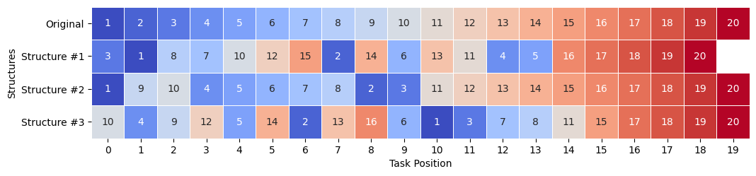
We observe that all candidates are similarly long and only Structure #1 is missing function 9, namely the one responsible for setting up random encounters, setup_interactions_random.
Regarding their commonalities, functions 17 (final_judgement_evaluation) and 18 (for_monitoring) are always in the same position, indicating a key role in the model performance. Indeed, function 18 calculates and updates the variable we ask PyNetLogo to report. Specifically, the overlap and order are noteworthy: 17 and 18 are the only overlaps that Structure #1 has with the original. Meanwhile, Structure #2 overlaps with the original for functions 1, 11, 12, 13, 14, 15, 16, 17, and 18. Structure #3 has the same order of overlap with the original in functions 7, 8, 17, and 18.
Recall that the candidates have been selected to have the maximum pairwise distance (calculated as 14). We can further measure the difference from the original and obtain 16, 6, and 17, respectively. This variability shows that both little and significant distances can lie between well-performing runs, i.e. the structure-fitness landscape is not very smooth.
Mapping each of the four runs from the function names to the category they belong to (“Letter” column in Table 6), we obtain Table 7 as a categorical overview. While the end, as observed before, is similar for all sequences, there are individual variations:
- Structure #1 alternates between several categories early on and continues with interleaved tasks. The middle third is more varied, too, as it introduces the evaluation functions.
- Structure #2 remains closest to the original, with a slight early deviation as it introduces setup and interaction steps earlier.
- Structure #3 is the most shuffled and divergent, with alternating task types right from the beginning, lacking any apparent clustering of updates or other task categories, making the early and middle sections heavily rearranged, suggesting a significantly different execution path.
- Regarding commonalities, all three candidates have none of the evaluation functions in the first third. Similarly, all sequences have at least some update steps in the first third. Lastly, all share a large diversity of tasks in the middle.
| Number | Task | Category | Letter |
|---|---|---|---|
| 1 | update_status_product |
update | u |
| 2 | update_awareness_list |
||
| 3 | update_complexity |
||
| 4 | update_compatiblity |
||
| 5 | update_relative_advantage |
||
| 6 | update_households_with_without_product_encountered |
||
| 7 | update_memory_minimum_time_between_2_decisions_ON |
||
| 8 | setup_interactions_neighbors |
setup | s |
| 9 | setup_interactions_random |
||
| 10 | check_for_awareness_of_interactions |
interaction | i |
| 11 | receive_information_from_interactions |
||
| 12 | make_final_judgment_enough_information |
judgement | j |
| 13 | evaluation_relative_advantage_product |
evaluation | e |
| 14 | evaluation_complexity |
||
| 15 | evaluation_compatibility |
||
| 16 | evaluation_observability_triability |
||
| 17 | final_judgement_evaluation |
other | o |
| 18 | for_monitoring |
||
| 19 | neighborlinks_die |
||
| 20 | randomlinks_die |
||
| Sequence | Abstraction |
|---|---|
| Original | uuuuuuussiijeeeeoooo |
| Candidate 1 | uusuijeueueiuueoooo |
| Candidate 2 | usiuuuusuuijeeeeoooo |
| Candidate 3 | iusjueueeuuuusieoooo |
The only function missing is setup_interactions_random in Candidate 1. This would raise questions about the necessity of additional random interactions between agents, which, in turn, adds more randomness overall to an already chaotic system.
Regarding real-world and case-related interpretation, the model functions do not allow direct insight into the theory used: The functions themselves represent the building blocks of the theory of Rogers (2014). They describe population-specific processes, i.e., processes executed for the entire population, less than denoting agent, agent-group, or agent-state-specific decision sub-processes or decision trees. This makes the theory resemble large-scale, averaging, continuous models rather than granular, individual-specific models that let phenomena emerge based on agent interactions. Thus, the model is more of an agent-based translation of the original economic theory.
While this poses demands for the design of ABMs made for structural calibration, an indirect interpretation is possible: For example, the function update_complexity is described in the model as “each household updates their knowledge of product complexity”. Say this function was missing from a structure. This could be interpreted as households having a fixed opinion about how complex a product is, so they do not change. This would link to the hassle of obtaining solar panels, their marketing, and the service provided.
In this light, we can only conjecture that even very different but well-performing structures will always need the same or similar building blocks and that more specification within the blocks is required. However, future research will have to confirm this as a stable trend and not a variable observation merely produced by chance. We believe that design demands for ABMs suitable for structural calibration would thus include a high degree of specificity and modularity. This will be discussed further later.
Limitations & Discussion
This research presents a way to generate, select, and evaluate structural modifications to an ABM using the inverse method for real-world data matching. It has exemplified its capabilities in a Dutch province-level solar panel adoption case study using a model of innovation diffusion. With this, the work presented connects to and enhances methodological approaches in inverse modelling and structural calibration of ABMs. The result is an open-source Python wrapper that coordinates the execution of this method on a NetLogo model. With this not being a fully fleshed-out case study, parameter calibration or robustness checks have not been conducted for this methodological contribution. Thus, the validity of what has been found and reliable behavioural interpretability is not given. Still, the case selected and considered is real and relevant and can serve as a guide for similar, more elaborate endeavours. Similarly, steps into case-specific interpretability have been taken by linking structural differences to the real-world ecosystem beyond the model. Were this result – the absence of the function update_complexity in a well-performing structure – achieved and validated through more extensive simulation, it would point investigations toward the question of how much the perception of complexity is fixed or can be influenced by external factors.
Our method in relation to the field
Our method needs to be contrasted with iGSS. We used iterative refinement of forward problems to match model output to real data. As such, our approach can be classified as inverse modelling. Still, it must be distinguished from iGSS, which combines primitives and operators to build fitness functions and resembles more symbolic regression. Meanwhile, we rearranged the order of and added or removed function calls to build new structures that make up one model iteration, thereby creating alternative models. Thus, both our and iGSS’s units are distinct in size, but the two methods are related in ends and goals: To discover new hypotheses and explain phenomena grown through the model. Thus, our structural inverse modelling approach is another take on the inverse method applied for ABMs and a self-standing concept next to iGSS.
Lastly, the work presented here on structural modification is relevant to the efforts around reusable building blocks (RBBs) and pattern-oriented modelling (POM). Grimm et al. (2022) define building blocks as “submodels describing processes that are relevant for a broad range of ABM in a certain application domain”, inferring a local generalisability and reusability to them beyond an individual model. Such standardised or reusable building blocks may improve validity, scrutiny, transparency and reproducibility of the ABM and its results (Lee et al. 2015), which are crucial for ABM applicability and use in, e.g. policy advice. Experiments with building blocks remain scarce because efforts to provide these in a standardised form and repository remain nascent. Most recently, this has been discussed through Berger et al. (2024), whose repository will soon be merged with agentblocks.org/. Indeed, the Python wrapper we designed proved useful in identifying bugs qua inter-block compatibility within the model utilised. Mutation options like “one-for-one exchanges” would enable effort-reduced testing of multiple behavioural theories in exchange like Muelder & Filatova (2018) did; this we take up in future work. Earlier, we advocated for size reduction and modularity as design principles. This may seem contradictory to the bigger blocks (Grimm et al. 2022) envisions and, thus, as a trade-off between building block variability through small, modular pieces and applicability through larger, comprehensive units. We think it is possible to go about this in two ways: One way would be to use building blocks as the smallest interaction pieces of a candidate model, similar to what we’ve done here. Another would be to use the approach laid out here for the granular calibration of one large building block. Indeed, our method would also be applicable using individual lines of code. In this way, the trade-off would be mitigated by explicitly focusing on the application and its scope.
Secondly, regarding POM, the method presented exhibits clear potential for structural inverse POM, so the structural calibration of a model using multiple patterns on different levels using inverse modelling. This application was not pursued in this study. This was decided for two reasons: the lack of suitable data (Epstein 2023) and models that align with this approach, and a deliberate focus on presenting the core methodological contributions without diverging into ancillary applications. Future research could explore the use of structural inverse POM on appropriate datasets, thereby expanding the applicability and robustness of the methods presented here and strengthening the link between existing ones. Furthermore, the multi-facetedness of POM may inform the debate on the structural sensitivity of the conclusions drawn. Multiple variables reported during structural variation may prove beneficial compared to one single variable to report.
Reflecting on our method
Related to POM, we must discuss the sensitivity aspects of our method design. Recall that we reported one single variable, the adoption of product 1, and used fast dynamic time warping to compare the similarity of the two curves. With this, the results are by design sensitive to the metric, and another metric like Hausdorff, local/global alignment, or shape-based similarity for time series or \(L^p\) for same-length arrays or functions may yield different results. This is worsened if the metric employed is not a metric in the mathematical sense and thus does not yield error-based comparability. Therefore, to decrease uncertainty, future work will have to increase metric adaptability to confirm or disprove this conjecture. Furthermore, with POM and quantifiable metrics, there is a chance of fixing the system in multiple variables and reducing uncertainty.
Concerning the nature of these error values generated by the metric, only time series alignment methods were usable to calculate the similarity of the model output (30 ticks) to the eight yearly adoption values from 2012 to 2019. This became an issue when investigating the overall good fit of Zuid-Holland and Noord-Holland in Figure 11. We hypothesised this to be due to these two curves being more shallow. Indeed, consider that the model only runs for thirty ticks. After that, the model can be more or less “done” with its municipal energy transition. The choice of 30 ticks was made to soft-code a cut-off point, i.e. avoiding merely partial but perfect fits, which would, due to shape dissimilarity, be punished with a high error value. Secondly, this choice was made due to the need to handle the computational and time constraints for evaluation. Based on this, many fundamental questions can be asked: How can (or should) the scarce, yearly data points be compared to the almost continuous model run? How do we deal with “predictive” fits beyond the real data? And why fast dynamic time warping, which does not satisfy the standardised definition of a metric like (pointwise) Euclidean distance? How does one single tick in the model relate to time in the real world and the data we utilise? These questions are key to real-world transfer and applicability, but also how to avoid overfitting of inverse modelling (Greig et al. 2023; Gunaratne et al. 2023).
Furthermore, we found the mutator instances to have trouble navigating the space of possibilities and finding suitable structures that produce a dynamic. Whether or not this is due to the abilities or design of the mutators (and if so, which) would need to be investigated more clearly in future work focused on hyperparameter tuning and implementing alternative methods. These results would both inform and have to be informed by the debate of how and to what extent to involve machine learning techniques in ABMs and social simulation in particular, cf. the work of Dahlke et al. (2020) or Ale Ebrahim Dehkordi et al. (2023). Alternatively, we see a possibility of leveraging a more exploratory and iterative use style that allows the balancing between structural exploration and parametric calibration, similar to an exploration-exploitation dynamic. Future work will pick this up.
At the same time, with an order of \(10^4\) structures explored out of the \(10^{20}\) possible ones, the exhaustiveness of the search space can only be called timid. This points in three directions for future work: Bigger mutation steps to increase possible coverage or smaller, well-thought-out experiments designed by the modeller and balancing between exploration and exploitation. Multiple steps, however, exponentially grow the option space and would therefore only be advisable if this came at a negligible cost. A third option, the application of adaptive genetic or learning algorithms, could bring alleviation with respect to the quality and density of the sampled subset within the search space. Still, given the computational costs of exploration, reducing the space to sample from appears inevitable.
Given the immense size of the joint structure-parameter-seed space, large-scale computational approaches seem inevitable even with the above workarounds. For this, using NetLogo has proved difficult, especially when attempting to let the Python wrapper parallelise the Java-based application on a Linux-based high-performance cluster. While follow-up work can solve the issues around parallelisation, this would still mean that future work should consider taking computationally more feasible and integrative approaches like MESA (Kazil et al. 2020) or Julia.
Lastly, to perform merely two runs is a choice made early in the project that inhibits our ability to provide meaningful statistical support for deductions from the data we generated. However, the point was to show that it is possible to vary and evaluate model structures and that doing this matters. The code is set up so the modeller can easily add more runs per structure or more parameters to test from. This would be up to the individual researcher if they apply our proposed methodology.
Generalisability and interpretability
Concerning methodological applicability beyond our case, we believe the methodology and approach presented here are not limited to the energy transition. Instead, we think it would apply to any ABM that would benefit from structural exploration, regardless of the field. For a discussion on design requirements, we refer to the following subsection.
However, our approach to analysing the outcomes must be examined more critically. We showcased an exploratory analysis of the dataset created, pointing out key features of the data, and sorted the data into a rudimentary two-by-two arrangement based on fitness and plausibility. This was done for two reasons: Firstly, to show what other researchers employing this method might look out for when facing large amounts of data with no idea how to make sense of it (Collins et al. 2024). And secondly, the lack of general methods for sense-making prompted us to develop something to move forward with. The fitness-plausibility diagram has proven to work, enabling us to filter and sort the data into manageable subsets. For this, we have developed the pruning method in Appendix B, a reliable quantification of the cut-off point for the fitness values. However, this two-by-two distinction cannot be considered sufficient for a general methodology. Much groundwork will have to be done to enable sense-making, from analysis criteria for sorting and filtering the data to methodologies for qualitatively analysing and interpreting structures of interest. We see the sense-making process as an interdisciplinary effort, and we cannot stress the role of domain experts enough.
Lastly, we must discuss how assessing the structural components of a model provides better support for decision-making from an ethical perspective. Our approach is part of a paradigm shift where instead of having one “single model with no sense of how unique it may be” (Collins et al. 2024 cf. 3.71) to multiple models. This shift has ethical implications, too. Such multi-model decision support with structural scrutiny could improve transparency about the underlying assumptions and workings and allow quantifiability of related uncertainty. Despite the lack of a general methodology for these potentials, they are not at all enabled by advice given based on one model at a time, which may contain unchecked biases.
Meta discussion and implications
Firstly, we have hinted at requirements for model design, and we must return to this to discuss how inhibited our method is by the modeller’s skills, potentially introducing a layer of subjectivity and inconsistency. This research used a modularly set-up model with mere function calls in the iteration. However, as described in the paragraph on RBBs, our method would theoretically also be applicable to individual lines of code. Thus, with little restrictions on the architectural setup, the model must be designed to handle inevitable errors that certain structures may raise gracefully. Naturally, as with any model, the research result depends on the modeller’s programming skills. We find that proper variable initialisation, handling of data types and edge cases, function compatibility, and modifiability are essential ingredients in any programming endeavour. As such, they do not necessarily only apply to our approach but to modelling in itself. Thus, applying our method would not aggravate the layer of subjectivity and inconsistency.
Next, consider the distribution of the error values obtained. We observed the data as chaotic and non-normal, even in the well-behaved parts after pruning. For future research, this potentially demands non-standard methods like non-parametric tests or value transformations that could bring the distribution closer to normality. However, transformations have limitations and may not fully address the issue if the deviations are due to complex underlying structures, as may well be the case with ABMs. However, this point must be taken with two grains of salt: The data analysed are synthetic and not obtained through a real-world measuring process that would introduce normally distributed errors. This poses the question of how much normality, regularity, or what kind of overall distribution can be expected at all. Secondly, suppose the data indeed display the hypothesised level of complexity. In that case, one must ask whether purely error-based analysis alone is really the holy grail or merely one part of the puzzle.
Returning to complexity, consider the outcome robustness under seed variation. In the Sankey diagram (Figure 13), we observed that for each quadrant, there was at least one structure that produced one run in that quadrant and, in the other run, no dynamics at all. While such overlaps have yet to be investigated further and their probability quantified, it sheds yet another light on the prior discussion: It is important to ask what we want from an ABM regarding regularity, reliability, normality, or control when varying the computational seed. The possible range of displayable “deterministic chaos”, i.e., a large variety of unpredictable outcomes through a deterministic process, has deep connections to the model’s purpose and control, e.g. whether we aim to predict where the system goes or strive to understand the dynamics and respond to it. It is easy to dismiss a model that produces behaviour that is unreliable or can seemingly go anywhere as chaotic and, thus, not suitable for study; consider the double pendulum as an example of an equation-based system that can be “moulded” and controlled into each state and yet produce seemingly irrational curves.
Relating to that, we’ve also seen the closeness and sharp discontinuity of the structure-fitness landscape. While it is evident that particular minor changes could produce an utterly nonsensical structure, it is not absurd to expect other minor changes to yield no noticeable effects. In other words, while it is highly doubtful that structural modification should be well-behaved, the extent of discontinuity observed was surprising. The inability to discriminate between such changes of “equal distance” points to a need for either distance measures between structures in more context-informed ways or requirements on model design, see also Epstein (2023 p. 4.18 or footnote 55) who raise similar issues about distance between rules. Indeed, the model at hand proved challenging to utilise. This difficulty may have been caused by its functions being set up as big blocks of code that encompass many variable changes and updates. This, in turn, would point to a smaller, chunk-sized, more modular model setup that also makes the theory more explicit.
Conclusion
To conclude, an answer to the research question “How can inverse modelling be made to deal with and evaluate variable model structures?” has been proposed. This has been done by putting forward a Python wrapper that varies the structure of the model, i.e. its iterative rule. To embed this research in the broader context, consider the following points:
Firstly, we have shown that large-scale structural calibration is possible within our working definition of “structure”. We have connected this effort to and thus driven forward the inverse method for ABMs. This underscores the applicability and relevance of the inverse method as a tool for ABMing efforts, validation, and theory building.
Second, the method proposed here relates to reusable building blocks as both the code and the analysis allow for comparing same-purpose building blocks with different formalisations. However, instead of a top-down plug-and-play, the method presented here goes bottom-up from the model, as it merely utilises the building blocks of the model. Connecting structural calibration with the effort to provide and scrutinise reusable building blocks is a most promising future outlook.
Thirdly, insights into models relating to sensitivity and uncertainty have been gained, and a gateway has been opened to multi-modelling. Sense-making techniques must be developed further to be successfully applied for robust multi-model decision support and hypothesis generation in social science.
To conclude, much work remains to incorporate structural calibration with parameter tuning and seed variation, conceptually and computationally. Future work and efforts will involve adding joint structural-parametric calibration and robustness to unlock and enable a deeper focus on sense-making. Indeed, it is essential to realise that this is not just a computational self-purpose but to allow a generative transfer back into social science. After generating such an unobservably large amount of uncertainty-infused data, pattern mining may be a way forward to complement qualitative sense-making to make the process more reliable, replicable, and valid. However, future research must decide to what extent agent-based modelling will become a big-data science, as this opposes traditional parsimoniousness and self-limitation in ABM development.
Acknowledgements
We want to take the opportunity to thank the editor and the two anonymous reviewers for the extensive, sharp, and kind feedback that we feel greatly improved the quality of our manuscript.
This research has been made possible through funding by the Energy Transition Lab of TU Delft’s Faculty of Technology, Policy and Management.
Notes
- ABMs can hardly be formalised as a function capturing the dynamics and even if, only reversed with significant effort that we consider not economic. Indeed, for such a function \(f\), injectivity would be a logical necessity for reversibility: a function \(f\) is called injective if for any \(n, m\) in the domain of \(f\) there holds that if \(f(m) = f(n)\), one can conclude \(n=m\). This may not be given were the ABM formalised as a function.↩︎
- For a discussion on how this notion relates to validity, we refer to the discussion.↩︎
- GitLab link: gitlab.tudelft.nl/lschubotz/structural-sculpting/↩︎
- 4TU Repository doi:
10.4121/2792c03f-16a1-43a8-8150-111b0f91ec26↩︎ - Algorithm 1 shows 21 distinct functions that serve as the base ingredients for building a go function. We restrict ourselves to structures of lengths 15 to 21 to avoid go functions that are too short to be meaningful. The number of ways to arrange \(k\) distinct items out of 21 in order and without repetition is given by the permutation \(\tfrac{21!}{(21-k)!}\). Summing these up would give \(\sum_{k=15} ^{21} \tfrac{21!}{(21-k)!} \approx 1.4 \times 10^{20}\) possibilities.↩︎
Appendix A: Changes Made to the Original Model by De Wildt (2014)
This section contains a list of changes that have been made to the model of De Wildt (2014). The modified model is available in the repository that accompanies this publication. The original code is in the comments above the changed lines and can be restored by reverting these changes.
Firstly, the functions neighborlinks_die and randomlinks_die have been created. This was done to replace the lines ask neighborlinks [ die ] and ask randomlinks [ die ], respectively. While this did not prove to be necessary ex-post, this was kept in to provide a harmoniously functionalised go function.
Second, within the function check_for_awareness_of_interactions, there was a while-check whether the length of the temporary list of friends, neighbours, and random links was greater than zero. However, in some instances, that list was set to 0, which did not have a length. As a consequence, an additional is-list? check has been added.
Similarly and thirdly, the function for_monitoring had a similar issue. For the variables c1 to c5, the length of the list households_with_whom_interacted was used without an is-list? or is-string? check. Adding these checks to the function resolved the errors.
To the best of our knowledge, these changes do not affect model outcomes and are thus comparable with the original model and with each other.
Appendix B: Finding the Quantile Cut-Off Point per Province
Figure 8 shows that the extreme error values begin at a different quantile value for each province. This section elaborates on how this cut-off point is found.
By taking the derivative of the quantile curve, we can see where the rate of change is increasing drastically or, mathematically speaking, less or greater than a certain threshold. We can combine these points into intervals where the derivative is below or above the threshold. Because we want to know the cut-off point where the error value becomes too large, we take the first point of the intervals where the derivative exceeds the threshold. These are the \(x\) values that are returned.
The process is described as a pseudo-algorithm in Algorithm 2. Its results are showcased in Figure 15 for the provinces Drenthe and Zeeland, where the quantiles from 0.0 to 1.0 are put on the \(x\)-axis and the error values (in yellow) and the derivative values (in blue) on the \(y\)-axis. The cut-off points identified are marked with dashed vertical lines.
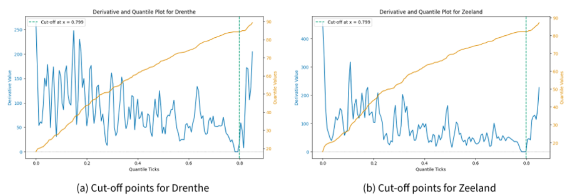
In the case of Drenthe, the choice is straightforward as it finds merely one point where the quantile curve “plateaus” before shooting up. In the case of Zeeland, the quantile values and the rate of change are so high towards the end that the curve appears almost flat. Yet, with the same threshold, we can identify three potential cut-off points. In such a case of multiple cut-off points, we have defaulted to taking the lowest cut-off point to remove the extreme outliers at the tail of the error distribution.
References
ALE Ebrahim Dehkordi, M., Lechner, J., Ghorbani, A., Nikolic, I., Chappin, E., & Herder, P. (2023). Using machine learning for agent specifications in agent-based models and simulations: A critical review and guidelines. Journal of Artificial Societies and Social Simulation, 26(1), 9. [doi:10.18564/jasss.5016]
AUGUSIAK, J., Van den Brink, P. J., & Grimm, V. (2014). Merging validation and evaluation of ecological models to “evaludation”: A review of terminology and a practical approach. Ecological Modelling, 280, 117–128. [doi:10.1016/j.ecolmodel.2013.11.009]
BALCI, O. (1998). Verification, validation, and testing. Handbook of Simulation.
BERGER, U., Bell, A., Barton, C. M., Chappin, E., Dreßler, G., Filatova, T., Fronville, T., Lee, A., Van Loon, E., Lorscheid, I., Meyer, M., Müller, B., Piou, C., Radchuk, V., Roxburgh, N., Schüler, L., Troost, C., Wijermans, N., Williams, T. G., … Grimm, V. (2024). Towards reusable building blocks for agent-based modelling and theory development. Environmental Modelling & Software, 175, 106003. [doi:10.1016/j.envsoft.2024.106003]
CARRERA, J., Alcolea, A., Medina, A., Hidalgo, J., & Slooten, L. J. (2005). Inverse problem in hydrogeology. Hydrogeology Journal, 13(1), 206–222. [doi:10.1007/s10040-004-0404-7]
CBS. (2019). StatLine - Zonnestroom; vermogen bedrijven en woningen, regio (indeling 2019). Available at: https://opendata.cbs.nl/#/CBS/nl/dataset/84783NED/table?dl=A84F3
CBS. (2024). StatLine - Huishoudens; samenstelling, grootte, regio, 1 januari. Available at: https://opendata.cbs.nl/statline/#/CBS/nl/dataset/71486ned/table?dl=A8542
COLLINS, A., Koehler, M., & Lynch, C. (2024). Methods that support the validation of agent-Based models: An overview and discussion. Journal of Artificial Societies and Social Simulation, 27(1), 11. [doi:10.18564/jasss.5258]
DAHLKE, J., Bogner, K., Mueller, M., Berger, T., Pyka, A., & Ebersberger, B. (2020). Is the juice worth the squeeze? Machine learning (ML) in and for agent-based modelling (ABM). arXiv preprint. arXiv:2003.11985 [doi:10.4324/9781003119128-14]
DAM, K. H., Nikolic, I., & Lukszo, Z. (2013). Agent-Based Modelling of Socio-Technical Systems. Dordrecht: Springer Netherlands.
DE Vries, G., Biely, K., & Chappin, E. (2021). Psychology: The missing link in transitions research. Environmental Innovation and Societal Transitions, 41, 42–44. [doi:10.1016/j.eist.2021.09.015]
DE Wildt, T. E. (2014). Supporting the adoption of smart grid appliances in city districts: A quantitative evaluation of policy options using agent-based modelling and scenario discovery. Available at: https://www.researchgate.net/publication/285596800_Supporting_the_adoption_of_smart_grid_appliances_in_city_districts_-_A_quantitative_evaluation_of_policy_options_using_agent-based_modelling_and_scenario_discovery
DHPC. (2024). DelftBlue supercomputer (Phase 2). Available at: https://n2t.net/ark:/44463/DelftBluePhase2
EDMONDS, B., & Moss, S. (2005). From KISS to KIDS - An “Anti-simplistic” modelling approach. In P. Davidsson, B. Logan, & K. Takadama (Eds.), Multi-Agent and Multi-Agent-Based Simulation (pp. 130–144). Berlin Heidelberg: Springer. [doi:10.1007/978-3-540-32243-6_11]
EPSTEIN, J. M. (1999). Agent-based computational models and generative social science. Complexity, 4(5), 41–60. [doi:10.1002/(sici)1099-0526(199905/06)4:5<41::aid-cplx9>3.3.co;2-6]
EPSTEIN, J. M. (2023). Inverse generative social science: Backward to the future. Journal of Artificial Societies and Social Simulation, 26(2), 9. [doi:10.18564/jasss.5083]
ERDEMIR, A., Mulugeta, L., Ku, J. P., Drach, A., Horner, M., Morrison, T. M., Peng, G. C. Y., Vadigepalli, R., Lytton, W. W., & Myers, J. G. (2020). Credible practice of modeling and simulation in healthcare: Ten rules from a multidisciplinary perspective. Journal of Translational Medicine, 18(1), 369. [doi:10.1186/s12967-020-02540-4]
GORE, R. J., Lynch, C. J., & Kavak, H. (2017). Applying statistical debugging for enhanced trace validation of agent-based models. SIMULATION, 93(4), 273–284. [doi:10.1177/0037549716659707]
GRAEBNER, C. (2018). How to relate models to reality? An epistemological framework for the validation and verification of computational models. Journal of Artificial Societies and Social Simulation, 21(3), 8. [doi:10.18564/jasss.3772]
GREIG, R., Major, C., Pacholska, M., Bending, S., & Arranz, J. (2023). Learning interpretable logic for agent-Based models from domain independent primitives. Journal of Artificial Societies and Social Simulation, 26(2), 12. [doi:10.18564/jasss.5087]
GRIMM, V., Berger, U., & Filatova, T. (2022). Reusable building blocks for agent-based modelling: Benefits, challenges, and a template for their release. Available at: https://scholarsarchive.byu.edu/cgi/viewcontent.cgi?article=4685&context=iemssconference
GRIMM, V., Johnston, A. S. A., Thulke, H.-H., Forbes, V. E., & Thorbek, P. (2020). Three questions to ask before using model outputs for decision support. Nature Communications, 11(1), 4959. [doi:10.1038/s41467-020-17785-2]
GRIMM, V., & Railsback, S. F. (2012). Pattern-oriented modelling: A “multi-scope” for predictive systems ecology. Philosophical Transactions of the Royal Society B: Biological Sciences, 367(1586), 298–310. [doi:10.1098/rstb.2011.0180]
GRIMM, V., Revilla, E., Berger, U., Jeltsch, F., Mooij, W. M., Railsback, S. F., Thulke, H.-H., Weiner, J., Wiegand, T., & DeAngelis, D. L. (2005). Pattern-oriented modeling of agent-based complex systems: Lessons from ecology. Science, 310(5750), 987–991. [doi:10.1126/science.1116681]
GUNARATNE, C., Hatna, E., Epstein, J. M., & Garibay, I. (2023). Generating mixed patterns of residential segregation: An evolutionary approach. Journal of Artificial Societies and Social Simulation, 26(2), 7. [doi:10.18564/jasss.5081]
HENDRICKS Franssen, H. J., Alcolea, A., Riva, M., Bakr, M., van der Wiel, N., Stauffer, F., & Guadagnini, A. (2009). A comparison of seven methods for the inverse modelling of groundwater flow. Application to the characterisation of well catchments. Advances in Water Resources, 32(6), 851–872. [doi:10.1016/j.advwatres.2009.02.011]
JAXA-ROZEN, M., & Kwakkel, J. H. (2018). PyNetLogo: Linking NetLogo with Python. Journal of Artificial Societies and Social Simulation, 21(2), 4. [doi:10.18564/jasss.3668]
JENSEN, T., & Chappin, E. J. L. (2017). Automating agent-based modeling: Data-driven generation and application of innovation diffusion models. Environmental Modelling & Software, 92, 261–268. [doi:10.1016/j.envsoft.2017.02.018]
KAZIL, J., Masad, D., & Crooks, A. (2020). Utilizing Python for agent-based modeling: The Mesa framework. In R. Thomson, H. Bisgin, C. Dancy, A. Hyder, & M. Hussain (Eds.), Social, Cultural, and Behavioral Modeling (pp. 308–317). Cham: Springer International Publishing. [doi:10.1007/978-3-030-61255-9_30]
KURAHASHI, S. (2018). Model prediction and inverse simulation. In S. Kurahashi & H. Takahashi (Eds.), Innovative Approaches in Agent-Based Modelling and Business Intelligence (pp. 139–156). Berlin Heidelberg: Springer. [doi:10.1007/978-981-13-1849-8_11]
KURAHASHI, S., Minami, U., & Terano, T. (1999). Why not multiple solutions: Agent-based social interaction analysis via inverse simulation. IEEE SMC'99 Conference Proceedings. 1999 IEEE International Conference on Systems, Man, and Cybernetics (Cat. No.99CH37028) [doi:10.1109/icsmc.1999.825315]
LEE, J.-S., Filatova, T., Ligmann-Zielinska, A., Hassani-Mahmooei, B., Stonedahl, F., Lorscheid, I., Voinov, A., Polhill, G., Sun, Z., & Parker, D. C. (2015). The complexities of agent-based modeling output analysis. Journal of Artificial Societies and Social Simulation, 18(4), 4. [doi:10.18564/jasss.2897]
MIRANDA, L., Garibay, O. O., & Baggio, J. (2023). Evolutionary model discovery of human behavioral factors driving decision-Making in irrigation experiments. Journal of Artificial Societies and Social Simulation, 26(2), 11. [doi:10.18564/jasss.5069]
MITCHELL, S. D. (2009). Unsimple Truths: Science, Complexity, and Policy. Chicago, IL: University of Chicago, IL: Press.
MUELDER, H., & Filatova, T. (2018). One theory - many formalizations: Testing different code implementations of the theory of planned behaviour in energy agent-Based models. Journal of Artificial Societies and Social Simulation, 21(4), 5. [doi:10.18564/jasss.3855]
MURRAY-SMITH, D. J. (2000). The inverse simulation approach: A focused review of methods and applications. Mathematics and Computers in Simulation, 53(4), 239–247. [doi:10.1016/s0378-4754(00)00210-x]
NAUMANN-WOLESKE, K., Knicker, M. S., Benzaquen, M., & Bouchaud, J.-P. (2022). Exploration of the parameter space in macroeconomic agent-based models. arXiv preprint. arXiv:2111.08654 [doi:10.2139/ssrn.3964901]
PAYETTE, N. (2024). The curse of possibilities. In C. Elsenbroich & H. Verhagen (Eds.), Advances in Social Simulation (pp. 601–608). Cham: Springer International Publishing. [doi:10.1007/978-3-031-57785-7_46]
REUILLON, R., Leclaire, M., & Rey-Coyrehourcq, S. (2013). OpenMOLE, a workflow engine specifically tailored for the distributed exploration of simulation models. Future Generation Computer Systems, 29(8), 1981–1990. [doi:10.1016/j.future.2013.05.003]
ROGERS, E. M. (2014). Diffusion of Innovations. New York, NY: Free Press.
SALVADOR, S., & Chan, P. (2007). Toward accurate dynamic time warping in linear time and space. Intelligent Data Analysis, 11(5), 561–580. [doi:10.3233/ida-2007-11508]
SARGENT, R. G., & Balci, O. (2017). History of verification and validation of simulation models. 2017 Winter Simulation Conference (WSC). [doi:10.1109/wsc.2017.8247794]
TAVENAR, R. (2021). An introduction to Dynamic Time Warping. Available at: https://rtavenar.github.io/blog/dtw.html
TEN Broeke, G., van Voorn, G., & LigTENberg, A. (2016). Which sensitivity analysis method should I use for my agent-based model? Journal of Artificial Societies and Social Simulation, 19(1), 5. [doi:10.18564/jasss.2857]
TERANO, T. (2007). Exploring the vast parameter space of multi-agent based simulation. In L. Antunes & K. Takadama (Eds.), Multi-Agent-Based Simulation VII (pp. 1–14). Berlin Heidelberg: Springer. [doi:10.1007/978-3-540-76539-4_1]
TIAN, X. (2023). General-purpose inverse modeling framework for energy transition applications based on adjoint method and operator-based linearization. Delft University of Technology, PhD Thesis. [doi:10.2118/212169-ms]
UDRESCU, S.-M., & Tegmark, M. (2020). AI Feynman: A physics-inspired method for symbolic regression. Science Advances, 6(16), eaay2631. [doi:10.1126/sciadv.aay2631]
VU, T. M., Buckley, C., Duro, J. A., Brennan, A., Epstein, J. M., & Purshouse, R. C. (2023). Can social norms explain long-term trends in alcohol use? Insights from inverse generative social science. Journal of Artificial Societies and Social Simulation, 26(2), 4. [doi:10.18564/jasss.5077]
WIJERMANS, N., Boonstra, W. J., Orach, K., Hentati‐Sundberg, J., & Schlüter, M. (2020). Behavioural diversity in fishing - Towards a next generation of fishery models. Fish and Fisheries, 21(5), 872–890. [doi:10.1111/faf.12466]
WILENSKY, U. (1999). NetLogo. Center for Connected Learning and Computer-Based Modeling, Northwestern University, Evanston, IL.
WILLIGENBURG, A., Keijzer, K., & Avdic, N. (2023). Monitor Zon-PV 2023. Available at: https://open.overheid.nl/documenten/42664b4a-4d81-44ff-a5c6-5b84783b5f60/file
ZHANG, J., Ballas, D., & Liu, X. (2023). Neighbourhood-level spatial determinants of residential solar photovoltaic adoption in the Netherlands. Renewable Energy, 206, 1239–1248. [doi:10.1016/j.renene.2023.02.118]
ZHANG, Y., Pichon, L., Roux, S., Pellegrino, A., Simonneau, T., & Tisseyre, B. (2024). Why make inverse modeling and which methods to use in agriculture? A review. Computers and Electronics in Agriculture, 217, 108624. [doi:10.1016/j.compag.2024.108624]