Improving Contact Tracing by Prioritizing Influential Spreaders Identified Through Socio-Demographic Characteristics

aUniversity of Stuttgart, Germany
Journal of Artificial
Societies and Social Simulation 28 (4) 9
<https://www.jasss.org/28/4/9.html>
DOI: 10.18564/jasss.5761
Received: 22-Sep-2023 Accepted: 08-Oct-2025 Published: 31-Oct-2025
Abstract
To mitigate the spread of contagious diseases, there is an ongoing discussion surrounding interventions that strategically target individuals who, due to their social network position, are responsible for more infections than others. However, the practical identification of these individuals using conventional network metrics is considerably challenging due to the lack of required data. A potential remedy to this quandary is the development of easily observable proxy metrics for measuring influential spreading. This study aims to assess the viability of such an approach using the example of contact tracing. Utilizing an empirically calibrated agent-based model, the study investigates the extent to which the efficacy of contact tracing can be enhanced by prioritizing influential spreaders, identified using age and household size as proxy measures. The results reveal that the effectiveness of contact tracing is significantly influenced by whose contacts are traced. When the contacts of those causing the most infections are traced, it can substantially enhance the efficacy of contact tracing, even when they are identified solely based on proxy metrics such as age and household size. For the examined case of the German state of Baden-Württemberg, it appears that middle-aged individuals residing in larger households are responsible for most infections. Therefore, prioritizing contact tracing for this specific demographic group seems to be a robust strategy to improve contact tracing. Overall, the results support the potential of the proposed approach to reduce the overall societal costs of non-pharmaceutical interventions while increasing their impact. Further empirical testing of the approach appears worthwhile.Introduction
Pandemics are among the most significant challenges for modern societies. Besides the direct damage to people’s health, there are enormous societal consequences due to, for instance, overburdened healthcare systems or the unintended side-effects of non-pharmaceutical interventions (NPIs). During the COVID-19 pandemic, for example, rigid NPIs saved many lives on the one hand, but on the other hand, they also had a strong negative impact on the economy, labor markets, people’s physical and mental health (Bradbury‐Jones & Isham 2020; Brooks et al. 2020; Coibion et al. 2020; Lippi et al. 2020; Nishi et al. 2020; Polyakova et al. 2020; Sharma et al. 2021). Given that pandemics are more likely to occur in the future (Dodds 2019; Keesing et al. 2010), it appears necessary to develop efficient counter-measures that have a high negative impact on the number of infections while having a low negative impact on people’s quality of life and economic prosperity.
The intention to develop efficient counter-measures to fight the spread of infectious diseases is not new, but its importance was again highlighted due to the appearance of COVID-19. One often repeated suggestion is the development of highly targeted counter-measures that focus only on parts of the population with the most significant impact on the spread of the infectious disease due to their specific network position or behavior (Dezső & Barabási 2002; Herrmann & Schwartz 2020; Manzo & van de Rijt 2020; Nunner et al. 2022; Pastor-Satorras & Vespignani 2002; Pellis et al. 2015; Vermeulen et al. 2021; Wei et al. 2022; Woolhouse et al. 1997). The broad idea is to identify such influential spreaders using some measure of node influence and then alter the network structure in order to reduce their impact on the course of the pandemic.
However, although there are numerous methods to identify influential nodes in a (social) network at hand1 (Zhu & Wang 2021), the approach appears unfeasible in real-world epidemics (Nunner et al. 2022; Pellis et al. 2015). In most cases, it is simply impossible to measure node influence in the context of a spreading disease because there is not enough data on the (potentially global) contact network in which the pathogen is spreading (Nunner et al. 2022; Pellis et al. 2015). Hence, to make that unquestionably promising approach of targeting highly influential spreaders feasible, it is further suggested to search for alternative characteristics, especially socio-demographic ones, that correlate with influential spreading and are easy to observe in the real world (Nunner et al. 2022; Pellis et al. 2015).
Until now, only relatively few studies exist testing this approach. There are, for instance, studies that show the usefulness of interventions that focus on certain occupations in the context of sexually transmitted infections (Mishra et al. 2012) or COVID-19 (Nunner et al. 2022). Other studies used age as a proxy measure for high degree and high vulnerability to test different prioritization strategies in the context of vaccination campaigns against COVID-19 and other respiratory infectious diseases (Bansal et al. 2006; Ben-Zuk et al. 2022; Bubar et al. 2021; Matrajt et al. 2021; Moore et al. 2021). Given the current state of research, it appears necessary to conduct more research testing the approach of focused interventions that rely on proxy measures of influential spreading (Pellis et al. 2015). This study aims to further investigate the potential of the suggested approach by extending the range of examined proxy measures and interventions. Using an empirically calibrated agent-based simulation model2, we investigate the potential of optimizing contact tracing (CT) by prioritizing influential spreaders. Those influential spreaders are identified using age and household size.
Examining the optimization of CT is especially interesting because of its high resource intensity. Although digital types of CT exist, in many countries, such as Germany, manual CT, in which local public health authorities interview the infected, trace their contacts, and monitor quarantine compliance, is still the predominant type of CT. In addition, in contrast to interventions like vaccinations, CT does not offer any protection to the infected but only to the contacts of the infected or the contacts of the contacts of the infected. Hence, known strategies like prioritizing the oldest to reduce hospitalizations, as it is effective for vaccination campaigns (Ben-Zuk et al. 2022; Bubar et al. 2021; Matrajt et al. 2021; Moore et al. 2021), appear to be insufficient in the context of CT.
This study uses age and household size as socio-demographic predictors to identify influential spreaders because they are easy to observe in the real world, thus ensuring the approach’s feasibility. In addition, there is research showing the importance of both variables regarding the vulnerability to infectious respiratory diseases (Cardoso et al. 2004; Hoebel et al. 2022; Martin et al. 2020; Nafilyan et al. 2021; Wachtler et al. 2020), which suggests that they might also be crucial to the spreading of contagious diseases. Furthermore, the existing research and data allow us to validate the simulation results concerning those two predictors partly.
Building on the foundations laid by Kaffai & Heiberger (2021), the agent-based model is calibrated to the federal state of Baden-Württemberg, Germany, and has a fine-grained micro-level representation with a representative distribution of agent attributes and a representative contact network. To attain a detailed representation of the micro-level, we construct the population of agents directly from the data of complete households of survey participants provided by the German Socio-Economic Panel (Goebel et al. 2019). Hence, many of the attributes of an agent (e.g., age, gender, working hours, economic sector) correspond to the characteristics of a specific survey participant. Furthermore, due to the data on complete households, the household composition for each agent is fully known so that the closest contact network can be modeled with a solid empirical foundation.
To ensure that the pathogen’s behavior in the simulation is as realistic as possible and based on current, comprehensive data, its characteristics were chosen with reference to the COVID-19 virus. However, COVID-19 serves solely as a reference for obtaining realistic parameter values. In a sensitivity analysis, we vary relevant pathogen properties to assess whether the results of our analysis also hold for pathogens with different characteristics.
The results support the potential of the proposed approach to increase the impact of counter-measures against infectious diseases. For Baden-Württemberg, age and household size seem suitable for singling out individuals who markedly contribute to escalated infection rates compared to others. Focusing CT efforts on these individuals can amplify the impact of CT measures significantly. However, when using the wrong prioritization strategy, the effectiveness of CT can also be dramatically decreased. Overall, it seems to make a big difference whose contacts are traced, and it is worth paying closer attention to which contacts are traced in order to protect the health of the population and use resources efficiently.
Methods
The goal of this study is to answer the question whether CT can be optimized by targeting only those individuals – and their contacts – that are identified as causing the most infections according to their age and household size. This research question affords a two-step analysis.
- The first step is to determine in what way age and household size can predict the number of infections caused. To investigate this relationship, we use an empirically-calibrated agent-based model which simulates the spread of an infectious disease within an agent population with realistic socio-demographic characteristics. We analyze the simulated micro-level data using a negative-binomial regression model.
- In a second step, we utilize the results from the first analysis step to extend the agent-based model with contact tracing that targets agents and their contacts according to their socio-demographic characteristics. In simulation experiments, we compare the efficacy of contact tracing under different prioritization strategies focused on age and household size.
The following sections provide details on the agent-based model, the implementation of the targeted contact-tracing, the validation and calibration procedures and the setup of the simulation experiments.
The agent-based model
The main part of the analyses in this study is conducted using an agent-based model based on an earlier model developed by Kaffai & Heiberger (2021) in the programming language Python. The model simulates the spread of a contagious disease in a society of people living their daily life. The main model procedures are agents visiting various locations, encountering other agents at those locations, infecting encountered agents, or becoming infected. Furthermore, the agents and the contacts of a selected proportion of agents can be traced and quarantined. In the following, the model components and mechanisms are described in detail.
Overview of the simulated entities
The artificial world of the agent-based model consists of three main entities: agents, locations, and pathogens.
- Agents represent people living their daily life, including various activities. The agent-specific daily schedule of performed actions depends on the individual characteristics of an agent (e.g., age, work hours, occupation, infection status) and the state of the global environment (e.g., time). The individual values of the agents’ attributes are mostly taken directly from the GSOEP, i.e., each agent represents a survey respondent in regard to their attributes. One of the most important properties of an agent is also a certain disease state. Agents can be, for instance, susceptible, infectious or immune. Furthermore, agents are able to remember whom they met and for how long during the past three days.
- Locations represent places where agents carry out their daily activities and engage in interpersonal interactions.3 The purpose of the locations in the model is to generate a realistic population-wide contact-network between the agents. The model incorporates various key locations, including individuals’ residences, workplaces, school classes, kindergarten groups, university seminars, supermarkets, places of social gathering, and venues for chance encounters. Agents are assigned to specific locations based on their attribute values. Each location has specific rules that define what conditions an agent must meet in terms of attribute values in order to be assigned to that location. Because most locations in the model bring together agents based on similar values on specific attributes, the main mechanism to generate edges between agents is homophily (McPherson et al. 2001). For instance, locations of the type work place are only visited by people working in the same economic sector, distinguished by the NACE Rev. 2 classification. Intra-location interactions between agents take place through a regular random graph, where the number of ties per agent is defined by the specific location rules. The size of a location in terms of assigned agents is determined either based on empirical micro data (GSOEP), average values taken from empirical macro data or based on reasonable assumptions.
- Pathogens represent a virus spreading through the artificial society of agents. The pathogen is transmitted with a calibrated probability from an infectious agent to a susceptible agent, if these agents encounter each other at a location. If an agent gets infected by the pathogen, it causes an infectious disease in the agent’s body and triggers a multistage disease process. Although the aim of this study is to produce results that are quite general for a wide range of infectious respiratory diseases, the properties of the pathogen and the disease process are oriented and calibrated to SARS-CoV-2 and COVID-19.
Initialization
The first step of each run of the simulation model is to initialize the population of agents based on survey data from the GSOEP (SOEP 2021). With approximately 30,000 individuals nested in nearly 15,000 households, the GSOEP provides representative data on socio-demographic characteristics, attitudes, and the everyday life of the German population. In addition, the GSOEP has one significant advantage over most other survey studies: It samples households and collects detailed individual data on every person living in that household. In this way, the GSOEP records the most important part of the social network (McPherson et al. 2006) for each person surveyed. This, in turn, allows us to reconstruct the most important parts of the overall social contact network – people living in households – directly from empirical data. For this study, we use the 2018 data collected only in the federal state of Baden-Württemberg to build a model that accounts for small-scale characteristics of the social structure (Buckee et al. 2021). As we construct the households of the agents from empirical households included in the GSOEP, we only use data from households where no household member has missing data on relevant variables. Thus, we exclude 1.21% of the 2018 Baden-Württemberg data due to missing values.
To create the population of agents, we draw a random sample (with replacement) of households from the GSOEP until a population size of 10,000 agents is reached. During this sampling procedure, we apply household level post-stratification weights adjusted for Baden-Württemberg. Each household of survey participants sampled from the GSOEP is used to create a household of agents, where each agent represents one household member. After creating the agent population, the set of locations is built. First, a home location is created for each agent household, where household members default to during the simulation. Locations of other types are built during the following routine: For each type of location, a set of rules determines which agents get assigned to this type of location based on the attributes of the agents. Based on the number of assigned agents and the location size, the number of locations of this type is calculated. When the set of locations is created, for each type of location, the agents are allocated randomly to one concrete location of each location type they are assigned to.4 Finally, before the main simulation loop starts, a subset of the agent population is selected randomly and exposed to the virus to start the pandemic. The amount of initially exposed agents proportionally reflects the age-specific 7-day-incidence rates empirically observed on the first simulated day (June 1, 2022) and is based on data by the Robert Koch Institute (Robert Koch Institut 2025).
Main simulation loop: Location visits, pathogen transmission and disease progression
Each simulation run simulates a period of two months of virus spreading (June and July 2022) in Baden-Württemberg. Each iteration of the main simulation loop represents one day. First, every agent visits those locations for a specified amount of time, which the agent is assigned to, and where the condition defined by the location is met for this day. When all agents are done with their daily visits, a weighted bipartite network of agents and locations is constructed based on the time an agent spends at each location. To determine who met who this day and calculate the corresponding duration of contact between two agents, the weighted bipartite network is projected into a weighted unipartite agent-to-agent network. The following procedure determines the contact duration: For each pair of agents, it is assessed whether they visited the same location that day and if they had contact with each other while visiting the same location. Whether they had contact with each other depends on the specific structure of the random regular graph within a location and the specific network position within that graph. If agent \(i\) and agent \(j\) had contact with each other on location \(l\), \(c_{ijl}\) is set to \(1\), otherwise, it is set to \(0\). The contact intensity between agent \(i\) and agent \(j\) at location \(l\) is then further determined either by:
| \[ w_{ijl} = c_{ijl} * \frac{ min(w_{il}, w_{jl})} {m}\] | \[(1)\] |
| \[ w_{ijl} = c_{ijl} * \frac{ w_{il} * w_{jl}} {m^2}\] | \[(2)\] |
Equation 1 is used if it is assumed that agent \(i\) and agent \(j\) visit location \(l\) simultaneously (e.g., classmates). Equation 2 is used if it is assumed that the agents visit the location independently from each other and at a completely random time of the day (e.g., people at the supermarket).
If agent \(i\) is in an infectious disease state and agent \(j\) is susceptible, the agent- and location-specific contact intensity \(w_{ijl}\) is used to determine a transmission probability \(p_{ij}\), in order to decide whether a transmission of the pathogen from agent \(i\) to agent \(j\) happens on that simulated day. The transmission probability \(p_{ij}\) is determined by:
| \[ p_{ij} = \sum_{l=0}^n w_{ijl} * t * s_{j}\] | \[(3)\] |
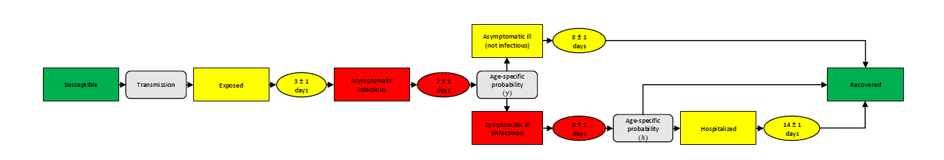
Every successful transmission triggers a multi-stage disease progression that includes exposed, asymptomatic infectious, symptomatic ill (infectious), asymptomatic ill (not infectious), severe symptoms (hospitalized), and recovered. The disease progression is based on Klüsener et al. (2020) and Kerr et al. (2021). To increase realism, for each agent, we add a random integer between -1 and 1 to each listed time span. Hence, every time span is an average value while the actual value for each agent can either last exactly the specified value, be one day shorter, or be one day longer, each with equal probability.
Figure 1 provides an overview of the possible courses of the disease. When the pathogen is successfully transmitted, the former susceptible agent is exposed to the virus. During this phase, the agent is neither infectious nor symptomatic. After an average of three days, an exposed agent becomes asymptomatically infectious for an average of two5 days. Subsequently, an age-specific probability determines whether the agent develops symptoms or not (see Table 1). In both cases, the agent stays infected for eight days on average. While symptomatic cases remain infectious, asymptomatic cases lose their infectivity again after the previous two-day infectious phase. We assume that symptomatic agents stay at home for the rest of the symptomatic phase to cure their symptoms. Asymptomatic ill agents turn into recovered agents after an average of eight days, while for symptomatic ill agents, there is an age-specific probability of developing severe symptoms with the necessity to be hospitalized (see Table 1). Since deaths are not considered in this model, we assume that even agents showing severe symptoms recover after a period of 14 days.
| 0–9 | 10–19 | 20–29 | 30–39 | 40–49 | 50–59 | 60–69 | 70–79 | 80–89 | 90+ | ||
|---|---|---|---|---|---|---|---|---|---|---|---|
| Susceptibility (\(s_j\)) | 0.34 | 0.67 | 1 | 1 | 1 | 1 | 1 | 1.24 | 1.47 | 1.47 | |
| Symptom probability (\(y\)) | 0.50 | 0.55 | 0.60 | 0.65 | 0.70 | 0.75 | 0.80 | 0.85 | 0.90 | 0.90 | |
| Hospitalization probability (\(h\)) | 0.00050 | 0.00165 | 0.00720 | 0.02080 | 0.03430 | 0.07650 | 0.13280 | 0.20655 | 0.24570 | 0.24570 | |
Intervention
The model as previously described can be considered as the base model in which no organized intervention against the spread of the infectious disease is implemented. In the following, we describe which further mechanisms are added to the model in order to implement targeted contact tracing.
In the case contact tracing is activated, a specific proportion of agents is selected as the prioritized agents before each simulation run. The proportion of agents selected as prioritized agents is systematically varied during the simulation experiments. The way those prioritized agents are selected is determined by the applied prioritization strategy. The baseline prioritization strategy selects a certain proportion of agents at random. All other prioritization strategies first sort the agents based on a specific agent attribute and then select a certain proportion of agents with the highest or lowest values on that attribute.6
The following list gives an overview of how the agents are prioritized in each strategy.
- Random: Randomly selected agents are prioritized. This strategy serves as the reference for all other strategies.
- HH+Age: Using Model 3 in Table 3, only those agents for whom the highest number of caused infections is estimated based on age and household size are prioritized.
- HH: Using Model 1 in Table 3, only agents for whom the highest number of caused infections is estimated based on household size are prioritized. Since it has been empirically shown that large and crowded households are a risk factor for infection with respiratory infectious diseases (Cardoso et al. 2004; Martin et al. 2020; Nafilyan et al. 2021), this strategy also has an empirical rationale.
- Age: Using Model 2 in Table 3, only agents within the age groups with the highest expected number of caused infections are prioritized.
- Inc. sim.: Only agents that are in the age groups with the highest COVID-19 incidence in the simulation (see Panel C in Figure 5) are prioritized. This strategy is based on the observation that the incidence within the age groups strongly correlates with the number of caused infections per age group. Since incidences are more observable empirically than the number of infections caused, and this information does not require simulated data, the approach could be significantly more practical and reliable.
- Inc. emp.: Only those agents that are in the age groups with the highest empirical COVID-19 incidence during the simulated period (see Panel C in Figure 5) are prioritized. This strategy further examines the strategy of targeting the age groups with the highest incidences by using empirical incidences.
- Young: Only the youngest agents are prioritized. Prioritizing the youngest people is a frequently discussed strategy for vaccination campaigns (Matrajt et al. 2021; Trad & El Falou 2022). Since this strategy does not target the most influential or the most vulnerable group of agents, it can be considered as an additional reference strategy to better assess the impact of the other strategies.
- Old: Only the oldest agents are prioritized. Prioritizing the oldest people is a common strategy within the context of vaccination campaigns to reduce hospitalizations (Ben-Zuk et al. 2022; Bubar et al. 2021; Matrajt et al. 2021; Moore et al. 2021).
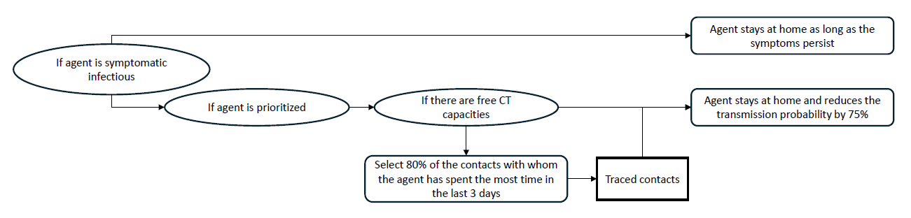
During the simulation, the infection status of all prioritized agents is monitored. As soon as a prioritized agent is showing symptoms, the contact tracing procedure is activated for this agent. The first step is to check whether there are still enough contact tracing capacities available. We allow a maximum of 500 tracings per 100,000 agents per 7 days.7 If the number of agents currently quarantined is smaller than this value, the following additional steps are executed: First, this agent stays at home for 10 days and the probability that this agent infects a household member during an encountering is reduced by 75%8 to model that the agent tries to isolate itself within the household. Subsequently, 80%9 of the contacts the prioritized agent had the most contact with during the last three days (today, yesterday, the day before yesterday) are identified. If there are enough CT capacities left, those identified agents are then isolated the same way as the prioritized agent: They stay at home for 10 days and the infection probability per encountering is reduced by 75%. Figure 2 visualizes the described intervention procedure. As shown in Figure 2, the self-isolation of symptomatic agents is an independent process carried out by all symptomatically ill agents, regardless of whether they are traced or not.
Replications and aggregation
Due to the stochastic components of the model, simulations are always executed in batches of 50 runs. For each batch, a population of 10,000 agents is created and used consistently across all 50 runs. While the agent population remains the same within each batch, the initially infected individuals are independently sampled in each run. After all replications within a batch have completed, agent-level attributes are averaged. As a result, each batch yields a single population of 10,000 agents with average values for attributes that are dynamically generated during the simulation (e.g., the number of infections caused directly or indirectly). During the calibration process, a single batch of 50 runs was sufficient to produce stable results when reproducing empirical case numbers (see Figure 10 in the Appendix). However, to obtain stable coefficients in the regression analysis, we use 30 different batches of 50 runs (see Figure 11 in the Appendix). In the simulation experiments that examine the efficacy of different contact tracing strategies, we use 50 such batches for each combination of parameters (see the Figures 12 and 13 in the Appendix).
Calibration and validation
The simulation model is validated and empirically calibrated mainly in respect to four different aspects: the distribution of agent-level and household-level characteristics, age-group-specific contact patterns, the number of COVID-19 cases over time and age-group-specific infection frequencies.
Population characteristics
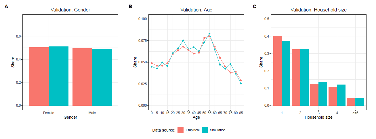
In order to ensure that the population of agents is representative for the real population of Baden-Württemberg, we validate the distributions of certain agent- and household-level attributes. Figure 3 compares the population of agents, which has been created based on the GSOEP, with empirical data on the population of Baden-Württemberg from the German Federal Statistical Office in regard to the distribution of age, gender, and household size. The characteristics of the simulated population closely match the empirical distributions.
Definition of locations
While the representativeness of characteristics at the agent and household level is ensured by using representative survey data, this is not the case for the representativeness of the contact network in the population. Rather, the contact network requires a calibration procedure which relies on the definition of the simulated locations. First, the most important places that people visit in their everyday lives were identified. These include households, age-group-specific kindergarten groups, age-specific school classes, university seminars, sector-specific workplaces and shops. In addition, unspecified places where friends meet and places where random contacts occur were included. Whenever possible, the characteristics of the places and the individual usage characteristics of the agents in relation to specific places were taken from the GSOEP. Otherwise, we rely on empirical average values or assumptions. Table 2 lists the locations and their attribute values. For all locations except households, there are two additional visit conditions: Agents do not visit the location if they are either currently quarantined or if they are symptomatic. Furthermore, for employed agents, a sector-specific probability based on Alipour et al. (2020) determines whether or not they work from home on a given day.
| Location | Nesting | Nodes | Degree | Affiliated agents | Visit days | Hours | Weight | |
|---|---|---|---|---|---|---|---|---|
| Home | Household-ID | Individual (SOEP 2021) | All | All | Everyday | Individual | Async. | |
| Kindergarten group 1 | None | 15 (Viernickel & Fuchs-Rechlin 2015) | 2 | 29.5% of aged 0-2 years (DESTATIS 2022a) | Mon.-Fri. | 6 (FDZ 2022) | Sync. | |
| Kindergarten group 2 | None | 15 (Viernickel & Fuchs-Rechlin 2015) | 2 | 94.5% of aged 3-5 years (DESTATIS 2022a) | Mon.-Fri. | 6 (FDZ 2022) | Sync. | |
| School class | Age | 25 (DESTATIS 2022b) | 2 | Agents aged 6-20 years | Mon.-Fri. | 6 (Destatis 2015) | Sync. | |
| Workplace | NACE Rev. 2 | 10 | 2 | Working agents aged > 20 | Mon.-Fri. | Ind. (SOEP 2021) | Sync. | |
| University seminar | None | 25 | 2 | Agents enrolled at university & aged > 20 | Mon.-Fri. | 4 (Destatis 2015) | Sync. | |
| Shop | None | 1000 | 2 | All | Mon.-Sat. | Ind. (SOEP 2021) | Async. | |
| Friends | age +/- 5 | 10 | 2 | All | Sat.-Sun. | 0.5 (Destatis 2015) | Sync. | |
| Random 1 | None | 10 | 6 | All | Everyday | 3 | Sync. | |
| Random 2 | None | 10 | 4 | Agents aged 15-60 years | Everyday | 2 | Sync. | |
| Random 3 | None | 10 | 2 | Agents aged 15-20 years | Everyday | 1 | Sync. | |
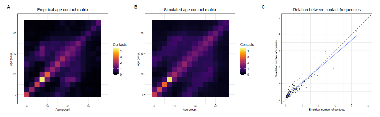
We compare the number of contacts made between different age groups in the simulation with empirical data on age-specific contacts (Prem et al. 2017) based on a contact survey conducted by Mossong et al. (2008). Since specific data for Baden-Württemberg are not available, data for all of Germany must be used at this point. Figure 4 shows the age-group-specific contact matrices and their correlation with one another. Each matrix shows the average number of contacts that one person/agent of a specific age-group has with each age-group per day. The main properties of the patterns of empirical contacts are replicated by the simulated contact network, as the comparison of Panel A and B in Figure 4 suggests. A Pearson’s R of 0.93 also indicates a good fit between the patterns of empirical and simulated data. However, since Pearson’s R only measures the relative match between the patterns of both data sources, it must be interpreted with caution. An additional chi-squared test also indicates that the difference between the two matrices is not statistically significant (\(\chi^{2}\) = 58.44, p=1, df=225). The congruence between the two contact matrices was predominantly established based on the empirically-informed definition of the locations of the type home, kindergarten groups, school classes, workplaces, university seminars, shops and friends. However, in order to enhance the correspondence between the simulated and empirical contact patterns, random contacts were incorporated in the model by defining the locations of type random until the presented level of alignment was achieved.
Transmission factor calibration and validation of infection dynamics
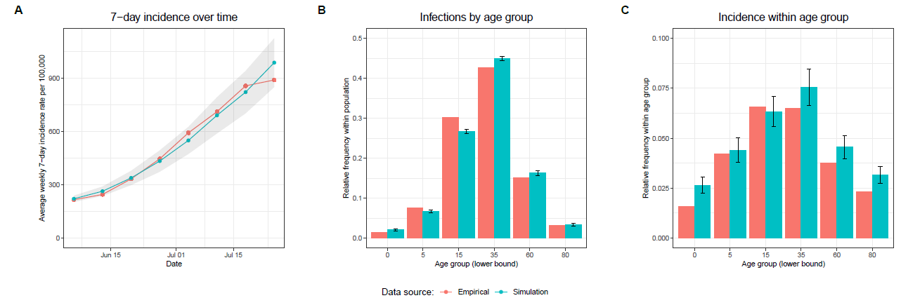
A sensitivity analysis (see Appendix) has shown that the results of the simulation experiments are sensitive to changes in the infection probability \(p_{ij}\). Although this does not affect the overall conclusion of the simulation experiments, only the absolute values of the summary statistics, it seems appropriate to set the infection probability into a realistic range. Thus, it was calibrated to data on the COVID-19 7-day incidence rate in Baden-Württemberg in June and July 2022. We chose this period because it was the beginning of one of the first waves of infections after almost all relevant restrictions were lifted in Baden-Württemberg. For the calibration procedure we used the Python package Optuna (Akiba et al. 2019). In multiple runs we allowed the transmission factor \(t\) to vary between 0 and 1 in order to broadly explore the parameter space. Based on this exploration we reduced the parameter space to the range between 0.32 and 0.34, in which we let the transmission factor \(t\) vary in further 150 trials with 50 replications each. Relying on the minimization of the sum of the root mean squared error between the simulated and the empirical weekly average 7-day incidence rate, we finally selected a transmission factor \(t\) of approximately 0.331195. Panel A in Figure 5 illustrates that after the calibration procedure the 7-day incidence rate per 100,000 produced by the simulation model is quite similar to the one calculated based on empirical data. It must be noted that in the simulation only symptomatic infections are counted as official infections to take into account that in reality the majority of asymptomatic infections stay undetected (Mahajan et al. 2021).
The infection dynamics are further validated by Panel B and C in Figure 5. Panel B in Figure 5 shows the number of infections by age-group as a proportion of the total number of infections within the population. Panel C shows the relative infection frequency within the age groups. Especially the distributions in Panel B show a close match between the empirical and the simulated age-specific infection numbers. Panel C also indicates a relative close match, but particularly in the group of the youngest and oldest there is a substantial overestimation by the simulation. However, these are the two smallest age groups with the smallest contribution to the total number of cases, and as Panel B in Figure 5 shows, this contribution to the total number of infections is satisfactorily captured by the simulation model. The close match between the simulated and empirical age-specific infection dynamics can also be considered as further validation of the contact network, as the structure of the contact network determines the propagation of a pathogen within and between the age-groups.
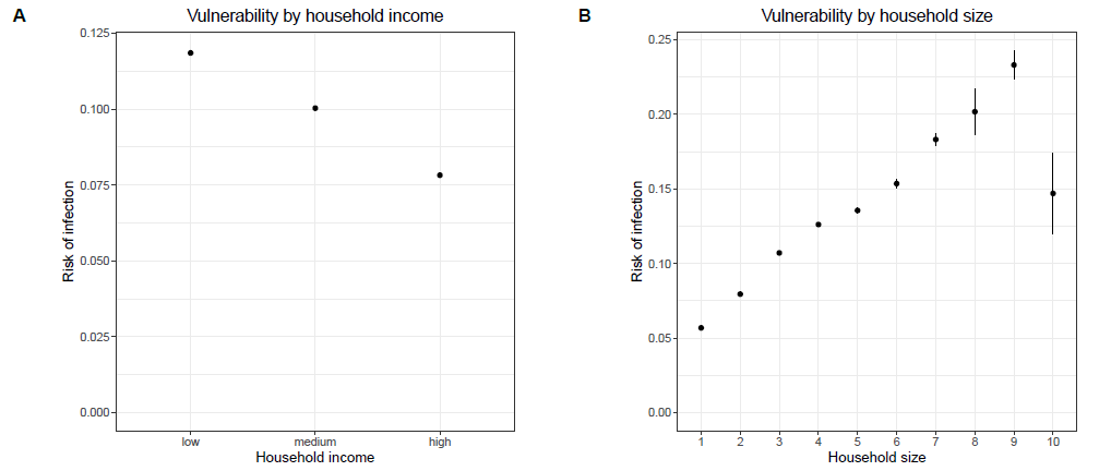
The infection dynamics of the model also exhibit a couple of properties which are known from the infection dynamics of COVID-19 and other respiratory diseases. The model reproduces these properties even though it was not explicitly calibrated to do so. One frequently described phenomenon is a negative relationship between the risk of an infection with COVID-19 and the socio-economic status (Hoebel et al. 2022; Wachtler et al. 2020). In line with that empirical observation, Figure 6 shows that the model produces a negative relation between equivalised household income and vulnerability to COVID-19: the higher the equivalised household income of an agent, the lower the probability of getting infected during the simulation run. Furthermore, studies show that being part of a large or crowded household is a risk factor for the infection with COVID-19 or any other respiratory disease (Cardoso et al. 2004; Martin et al. 2020; Nafilyan et al. 2021). As Figure 6 shows, the simulation model reproduces a positive correlation between household size and the vulnerability to COVID-19. The more agents live in a household, the higher is the risk of getting infected as a member of this household during the simulation.
Results
This section presents the results of the two-stage analysis. First, the regression model is used to answer which agents cause the most infections in the simulation. Next, the efficacy of different prioritization strategies developed based on the knowledge gained through the regression analysis is compared.
Who spreads most?
Table 3 presents the results of the negative binomial regression model with the number of infections caused as the outcome variable and age and household size as predictors. The outcome variable counts all infections that an agent caused directly or indirectly via other agents. In this case, all infections - symptomatic and asymptomatic ones - are counted, because at this point we are not interested in the number of officially detected infections one causes but in all infections one causes. Age is treated as a categorical variable with six categories (age groups: 1. 0-4, 2. 5-14, 3. 15-34, 4. 35-59, 5. 60-79, 6. 80+) following the classification of the Robert Koch Institute (Robert Koch Institut 2025).
| Dependent variable: | |||
|---|---|---|---|
| Number of caused infections | |||
| Model 1 | Model 2 | Model 3 | |
| Constant | 0.52*** | 0.53*** | 0.19*** |
| Household_size | 1.30*** | 1.28*** | |
| Age (Ref. 0–4): | |||
| 5–14 | 1.71*** | 1.62*** | |
| 15–34 | 2.89*** | 3.49*** | |
| 35–59 | 2.96*** | 3.75*** | |
| 60–79 | 1.19*** | 1.95*** | |
| 80+ | 0.62*** | 1.12*** | |
| Nagelkerke R2 | 0.111 | 0.153 | 0.228 |
| Observations | 300,000 | 300,000 | 300,000 |
| Note: | *p<0.1; **p<0.05; ***p<0.01 | ||
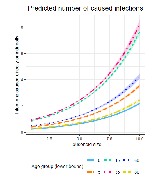
The regression analysis reveals that age and household size are relevant predictors of the ability to spread the simulated pathogen. As shown by Model 1, which includes only household size as a predictor, each additional household member increases the expected number of caused infections by a factor of 1.3 on average. Model 2 estimates that middle-aged agents cause the most infections, while the oldest and youngest are expected to cause the fewest infections. For instance, Model 2 indicates that the expected number of caused infections is, on average, increased by a factor of 2.96 for agents aged between 35 and 59 and increased by a factor of 2.89 for agents aged between 15 and 34 compared to the reference group of agents younger than five. In contrast, agents between 60 and 79 are expected to cause, on average, only 1.19 and agents older than 79 only 0.62 times as many infections as the reference group of agents younger than 5. Compared to household size, age has slightly greater predictive power, as indicated by the Nagelkerke R² values of 0.111 in Model 1 and 0.153 in Model 2. The predictive capability is further increased to 0.228 when combining the predictors in one model, as Model 3 indicates. Furthermore, the predominant role of the middle-aged groups and larger households persists in Model 3. Figure 7 illustrates the exponential nature of the relation between household size and the ability to spread. Figure 7 also indicates that the age groups have more minor differences concerning the number of caused infections in smaller households and larger differences in larger households.
It should also be noted that the order of the effect sizes per age group in Model 3 corresponds precisely to the order of the incidence rates per age group in the simulation (see Panel C in Figure 5 for comparison). Similarly, the positive relation between household size and the number of caused infections corresponds to the positive relation between household size and the risk of infection.
Optimizing contact tracing
The following section presents the results of the simulation experiments comparing various prioritization strategies. The experiments include eight strategies, each prioritizing certain agents in tracing their contacts in case of symptomatic infection.
Figures 8 and 9 present the performance of the different strategies as prevented infections and prevented infections per one tracing. In each figure, Panel A displays the mean performance for each strategy averaged across all proportions of prioritized agents, while Panel B shows each strategy’s performance at each tested proportion of prioritized agents.10
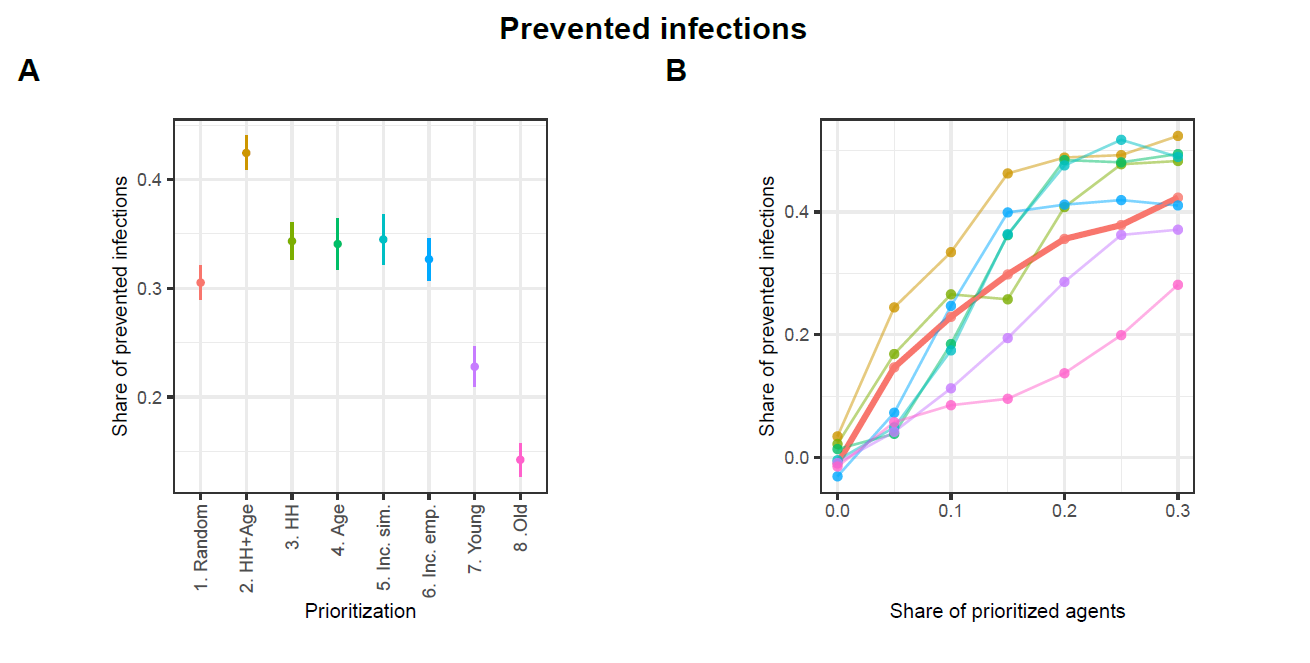
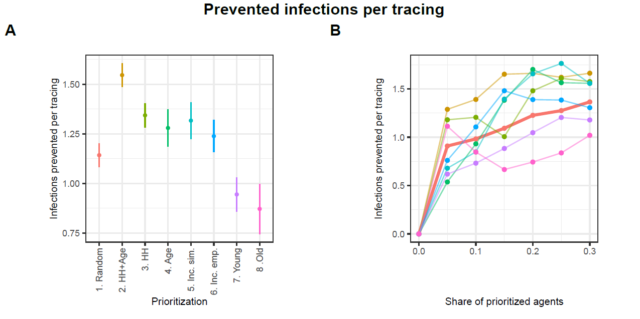
Figure 8 illustrates that all strategies can significantly mitigate the spread of infections. However, substantial variations exist among these strategies. Strategy HH+Age demonstrates the highest average share of prevented infections at approximately 42%. Hence, it outperforms the reference strategy Random, which prevents about 31% of infections, by about 11 percentage points. The alternative strategies HH, Age, Inc. sim., and Inc. emp. also yield higher levels of infection prevention, with reductions ranging between 33% and 34%, thereby demonstrating moderate improvements over the baseline. In contrast, the strategies Young and Old fall notably short in infection prevention, achieving approximately 23% and 14%, respectively.
Panel B in Figure 8 illustrates the performance of each strategy across varying proportions of prioritized agents. The share of prioritized agents has a strong positive effect on the number of infections prevented. For values below 20%, the HH+Age strategy clearly outperforms all others. The strategies HH, Age, Inc. sim., and Inc. emp. do not consistently outperform the Random strategy. However, when a larger share of agents is prioritized, the HH, Age, and Inc. sim. strategies achieve performance levels comparable to the HH+Age strategy. In contrast, the Young and Old strategies consistently perform worse than the reference strategy Random across all examined levels of prioritization.
Since the results presented in Figure 8 do not explicitly reflect the actual number of agents whose contacts are traced nor the exact number of committed tracings, Figure 9 shows the performances of the strategies relative to the number of executed tracings.11 Again, the HH+Age strategy performs best in total. While the reference strategy Random prevents approximately 1.1 infections per tracing, strategy HH+Age prevents approximately 1.5 infections per tracing. With values between 1.2 and 1.3 prevented infections per tracing, the strategies HH, Age, Inc. emp. and Inc. sim. are also substantially more effective than the Random strategy. With approximately 0.9 prevented infections per tracing, the Young and Old strategies continue to exhibit significantly lower effectiveness than the Random strategy.
Panel B in Figure 9 shows that although the HH+Age strategy achieves the highest overall efficiency, its advantage is particularly evident at lower levels of agent prioritization. At higher shares of prioritized agents, the HH, Age, and Inc. sim. strategies perform comparably to the HH+Age strategy. Interestingly, at a 5% prioritization level, not only does the HH strategy approximate the performance of HH+Age, but the Old strategy does as well. However, as the share of prioritized agents increases, the relative effectiveness of the Old strategy falls below that of the Random strategy. The Young strategy consistently performs worse than the Random strategy across all levels of prioritization.
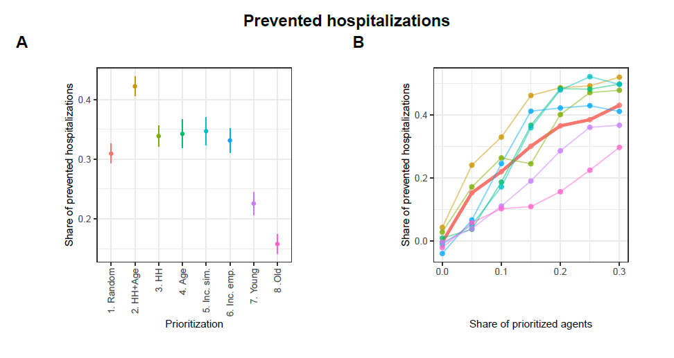
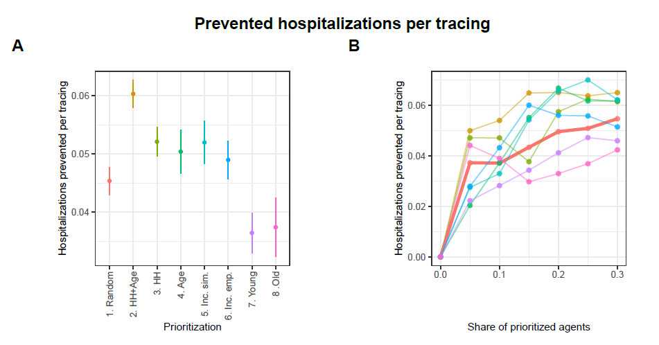
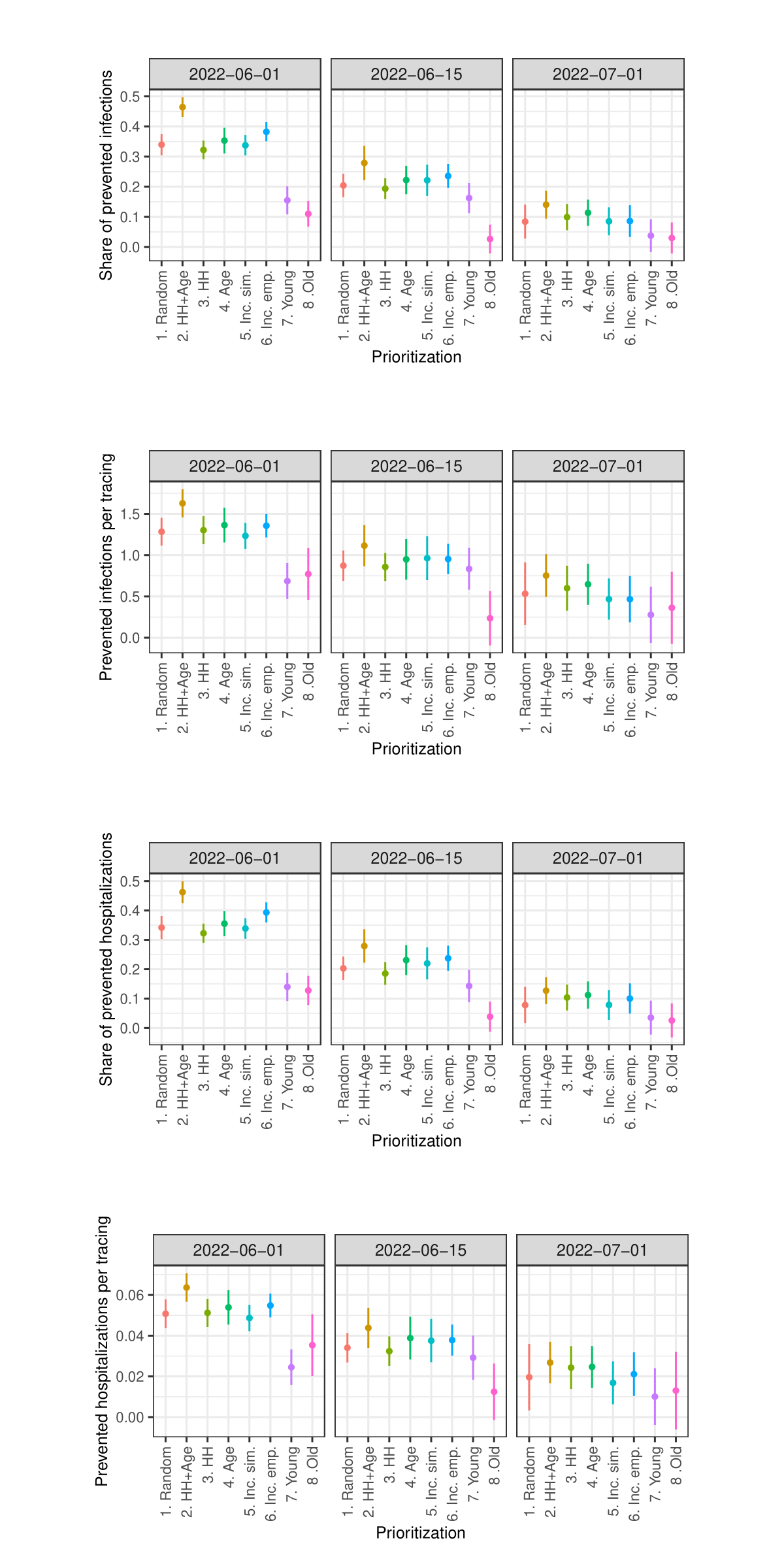
Figures 14 and 15 in the Appendix show the results concerning hospitalizations. Overall, the patterns described for prevented infections are similar to the patterns observed with regard to prevented hospitalizations. Particularly interesting here is that prioritizing the oldest agents also performs worst in terms of prevented hospitalizations, despite previous studies showing that prioritizing the oldest individuals in the context of vaccinations (e.g., against COVID-19) is most effective in preventing hospitalizations (Ben-Zuk et al. 2022; Bubar et al. 2021; Matrajt et al. 2021; Moore et al. 2021).12
Overall, the results clearly indicate that the most effective strategy is to prioritize contact tracing for individuals who, based on their age and household size, are estimated to cause the highest number of infections (HH+Age). Strategies that rely on a single predictor – either household size (HH) or age (Age) – also demonstrate promising results, though their performance gains are less consistent. A similar pattern is observed for strategies based on age-specific incidence rates (Inc. emp., Inc. sim.). In contrast, strategies that prioritize only the youngest agents (Young) or only the oldest agents (Old) — an approach commonly employed in vaccination campaigns — appear to be ill-suited for enhancing the effectiveness of contact tracing.
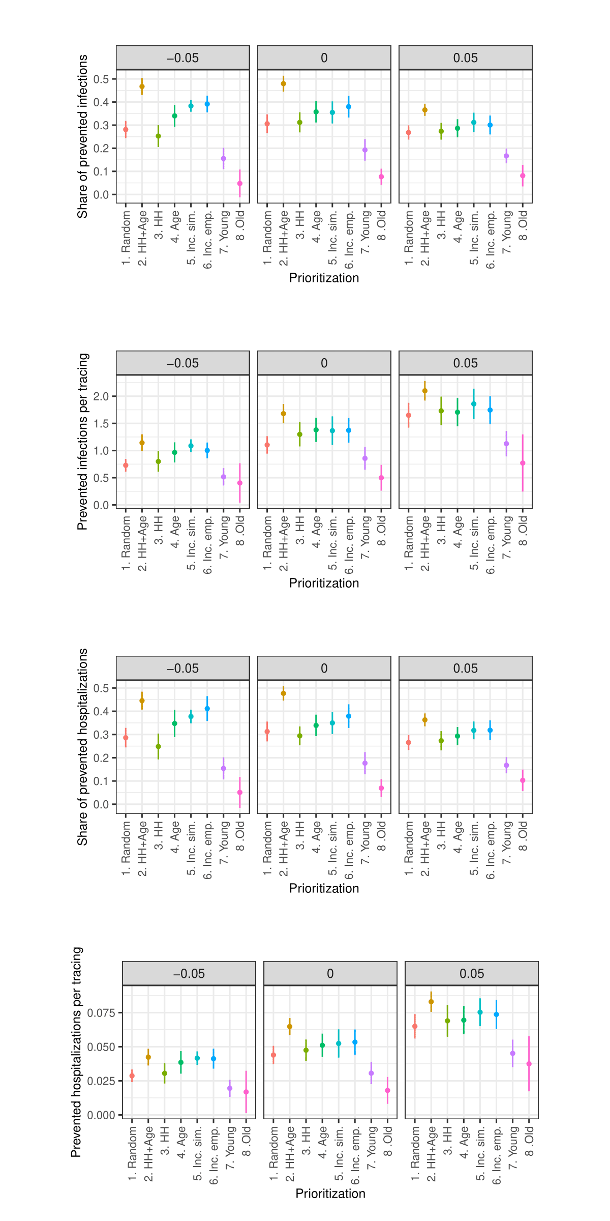
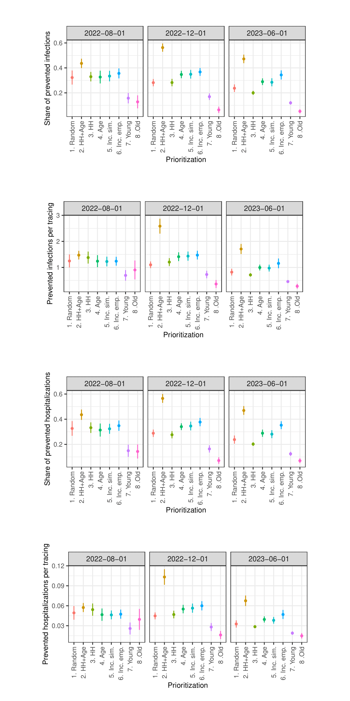
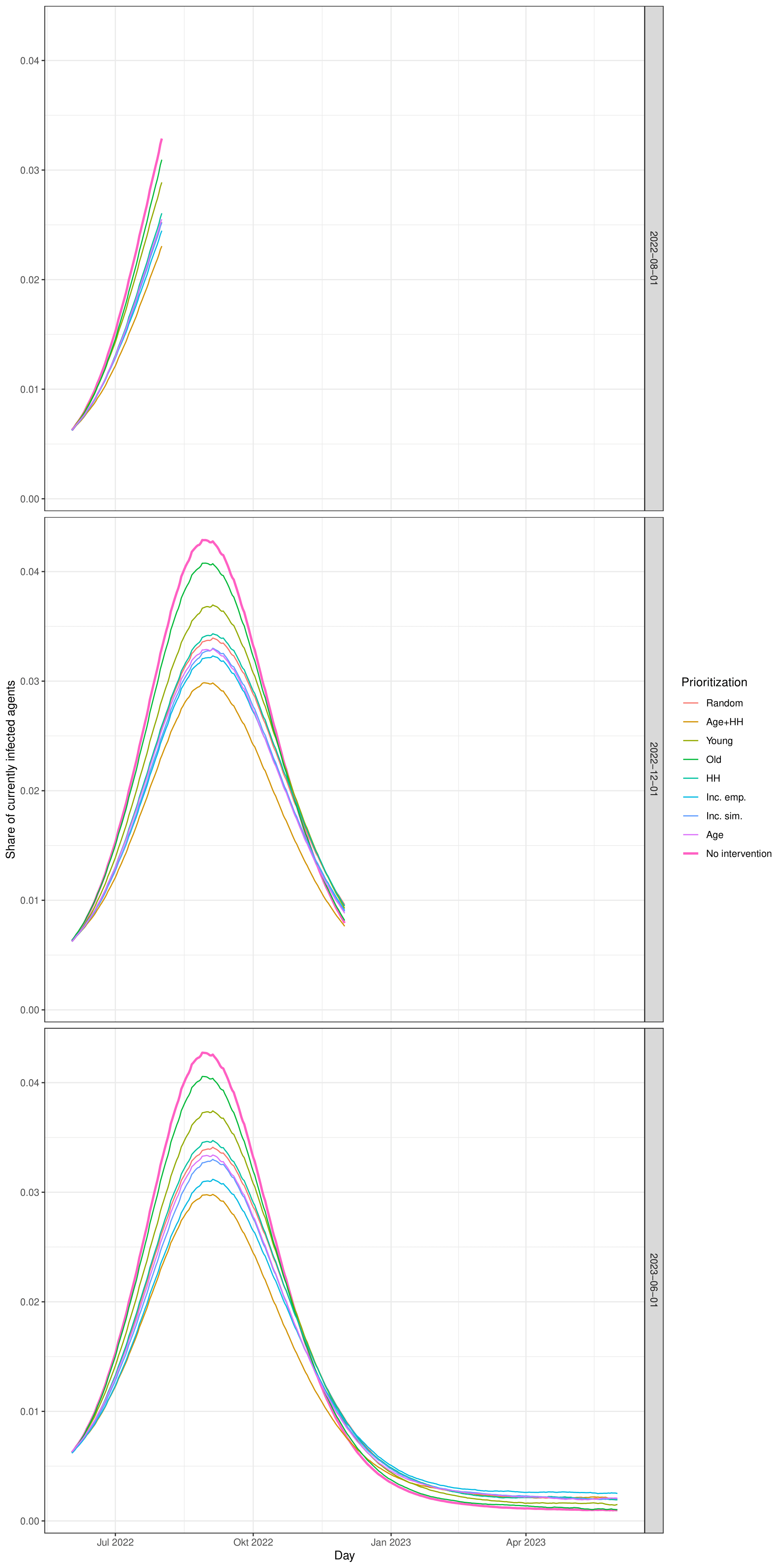
As the sensitivity analysis in the Appendix indicates, the results are sensitive to changes in parameters such as the length of quarantine, infection probability, duration of asymptomatic infectiousness, length of the simulated period, household isolation level, and timing of contact tracing onset. However, these changes primarily affect the overall magnitude of the outcomes rather than the relative ranking of strategies.
Conclusion
The overarching objective of the present study was to examine the extent to which measures aimed at combating the spread of infectious diseases can be optimized through a focus on high-spreading groups indirectly identified as such through proxy indicators. Such an approach aims to facilitate the identification of relevant groups even under actual pandemic conditions, where there is insufficient data available on the contact network through which the infectious disease spreads, rendering the calculation of traditional network metrics for identifying influential spreaders infeasible. In the present study, this approach was tested through the example of CT during the COVID-19 pandemic in Baden-Württemberg (Germany). The potential optimization of CT by focusing on the expected most influential spreaders identified based on age and household size was assessed through simulation experiments using an empirically calibrated agent-based model.
Based on the conducted simulation experiments, it can be reasonably stated that the effectiveness of CT is significantly influenced by whose contacts are traced. For the examined case of Baden-Württemberg, we find that middle-aged people (15-60 years) living in larger households cause the most infections. In the simulation experiments, tracing the contacts of these people was on average 1.4 times more effective both in terms of the absolute number of infections prevented and in terms of infections prevented per tracing than tracing the contacts of a random sample of people. Prioritizing agents solely by household size or age, as well as strategies focusing on the age groups with the highest number of infections, also proved to be significantly more effective than the reference strategy of selecting random agents. In particular, the latter strategies could be implemented in the real world, because incidence can be measured empirically without relying on simulation studies to gain information about who is causing the most infections. Remarkably, it appears that the strategy of prioritizing elderly individuals, which has been demonstrated as the most effective approach in preventing hospitalizations during COVID-19 vaccinations (Ben-Zuk et al. 2022; Bubar et al. 2021; Matrajt et al. 2021; Moore et al. 2021), does not seem to exhibit a significant improvement in the context of CT, but performs significantly worse when compared to a random selection of individuals. Thus, this study also shows that an improper prioritization strategy can cause great harm.
As this is a simulation study, it needs empirical research on actual applications of the tested approach to gain more reliable knowledge about its efficacy. The latter is particularly important since the present simulation study has several methodological issues. For instance, the simulated society in the model represents a closed system. Commuting, tourism, or migration, which can significantly impact the spread of an infectious disease, are not considered. However, the validation of infection dynamics shows that the modeled population groups and contacts are still sufficient to reproduce real infection dynamics adequately. Another issue is that the dataset used to calibrate the contact network is over a decade old and was not collected during times of an acute pandemic. Therefore, it is unclear to what extent the dataset can accurately represent current contact patterns. Nevertheless, this dataset still appears to be one of the best and most comprehensive data source regarding overall societal contact patterns. Due to uncertainties regarding the modeled contact patterns, the results concerning characteristics correlating with a high number of caused infections (the regression analysis) should be interpreted cautiously. That is especially true for the youngest and the oldest, as the simulation model systematically overestimates their incidences, possibly leading to overestimating the number of infections caused by them. Another area for improvement regarding age is that very few age groups with considerable differences in size are used in this study. More fine-grained age groups would lead to more precise results.
Our study may also underestimate the impact of prioritizing older adults, as it does not include long‐term care facilities where seniors have frequent interactions with many peers and elevated transmission risk. Instead, our model includes only community‐dwelling older individuals who maintain relatively few contacts. Therefore, the results concerning older adults in this study must be interpreted with the utmost caution.
When interpreting the results, one must also consider that in this simulation contact tracing is the only active intervention that interferes with the simulated spread of disease. In reality, contact tracing is often only used in scenarios where the current infection rates are at very low levels and furthermore often multiple interventions are active at the same time. For instance, as Bicher et al. (2021) show for Austria, even highly effective contact tracing can only play a minor role in disease containment. Thus, the simulation model might overestimate the impact of contact tracing in reality. However, the results regarding the relative differences between the strategies should hold even for such more realistic scenarios. This should be addressed in future research.
Despite several minor methodological limitations, this study is still able to demonstrate the following three points, listed in ascending order of uncertainty:
- The effectiveness of contact tracing is significantly influenced by whose contacts are traced.
- When the contacts of those causing the most infections are traced, it can substantially enhance the efficacy of contact tracing, even when they are identified solely based on proxy metrics such as age and household size.
- In the case of the German state of Baden-Württemberg, it appears that middle-aged individuals residing in larger households are responsible for most infections. Therefore, prioritizing contact tracing for this specific demographic group seems to be a promising strategy to improve contact tracing.
The implementation of the proposed targeted contact tracing strategy necessitates clarification of operational constraints, particularly with regard to testing capacities and the ability to trace and monitor quarantined individuals. These limitations define the subset of the population that can be classified as high-priority and thus targeted for intensified intervention. Identifying effective mechanisms to reach and engage this group — whether through appeals to individual responsibility via public communication strategies or through more systematic forms of surveillance — requires further interdisciplinary investigation and coordination with public health institutions. Crucially, any practical application of this approach must be accompanied by a thorough ethical evaluation. The potential for stigmatization and the imposition of quarantine based solely on socio-demographic attributes of contacts pose significant normative challenges (Brooks et al. 2020; Freytag et al. 2021; Saeed et al. 2020). Nonetheless, in situations where public health agencies face resource constraints and cannot trace all contacts comprehensively, prioritizing individuals whose isolation is likely to produce the highest epidemiological benefit may represent not only a more efficient, but also a more ethically defensible course of action.
Acknowledgments
This work was funded by Deutsche Forschungsgemeinschaft (DFG, German Research Foundation) under Germany´s Excellence Strategy – EXC 2075 – 390740016. The author acknowledges support by the state of Baden-Württemberg through bwHPC and the German Research Foundation (DFG) through grant INST 35/1597-1 FUGG.
The author gratefully acknowledges the valuable feedback and support of Raphael H. Heiberger and Lukas Erhard.
Appendix A: Evaluating the Number of Replications
This section evaluates whether the number of replications is sufficient to ensure stable model outputs. Each subsection shows how increasing replications reduces the variance of the average outputs until they stabilize.
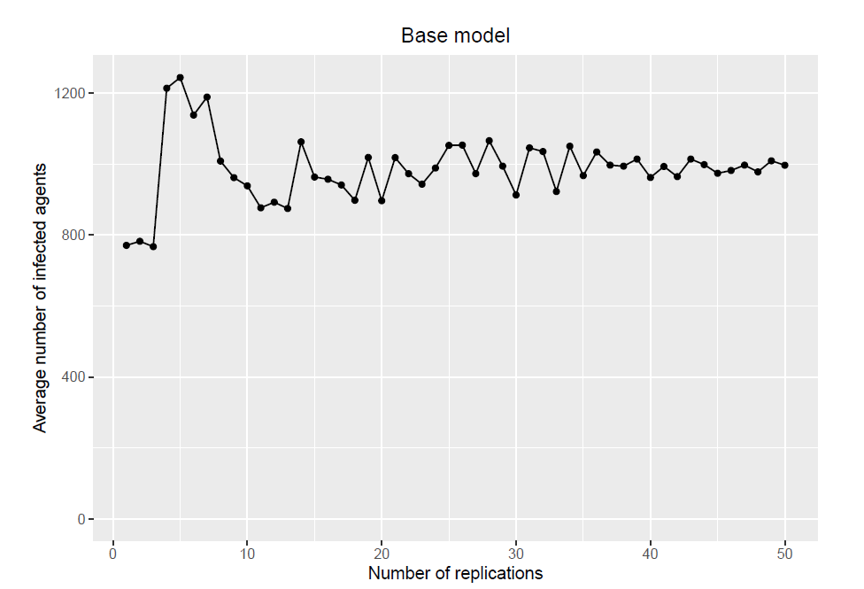
Base model
The base model consists of a population of 10000 agents and 50 replications. It creates one population and uses the same population for all 50 replications. Figure 10 shows how the average number of infected agents reaches a relatively stable state when approaching 50 replications.
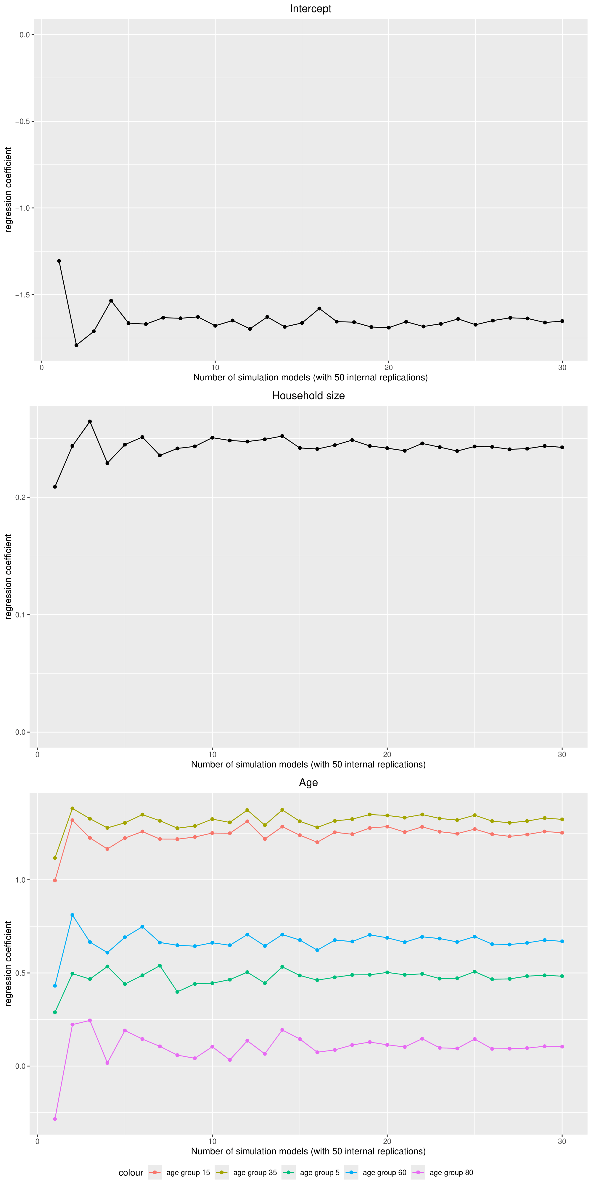
Negative binomial regression
Because the regression coefficients showed a substantial variation between different base models (with each 50 replications), the number of models was increased to 30. Figure 11 shows how the average regression coefficients reach a stable state when approaching 30 models (which are 1500 replications in total but with 30 different populations).
Experiments
To get stable results in the experiments, each scenario was computed with 50 models (which are 2500 replications per scenario). Figure 12 shows how the average number of infected agents per scenario approaches a relatively stable state with 50 models.
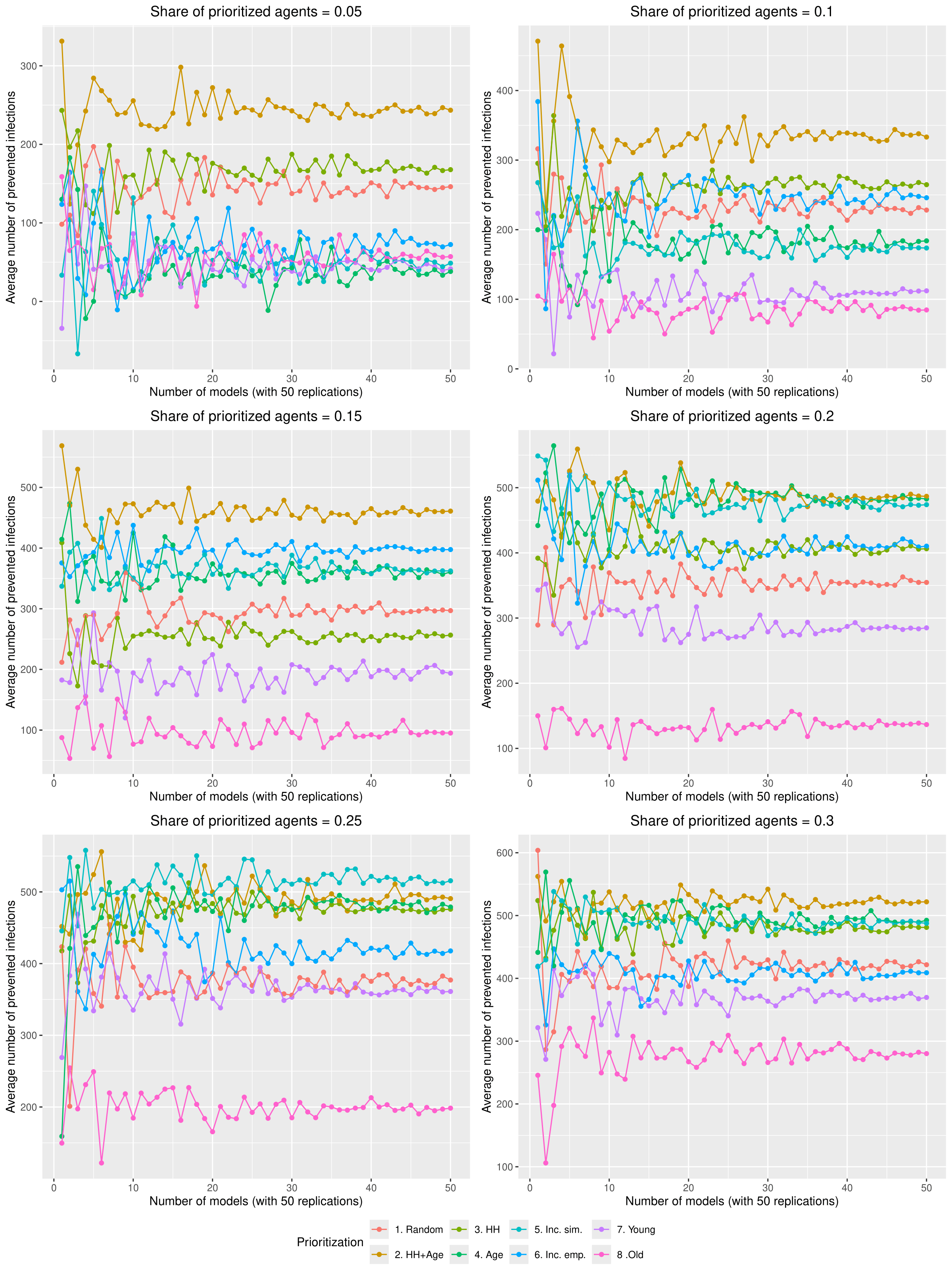
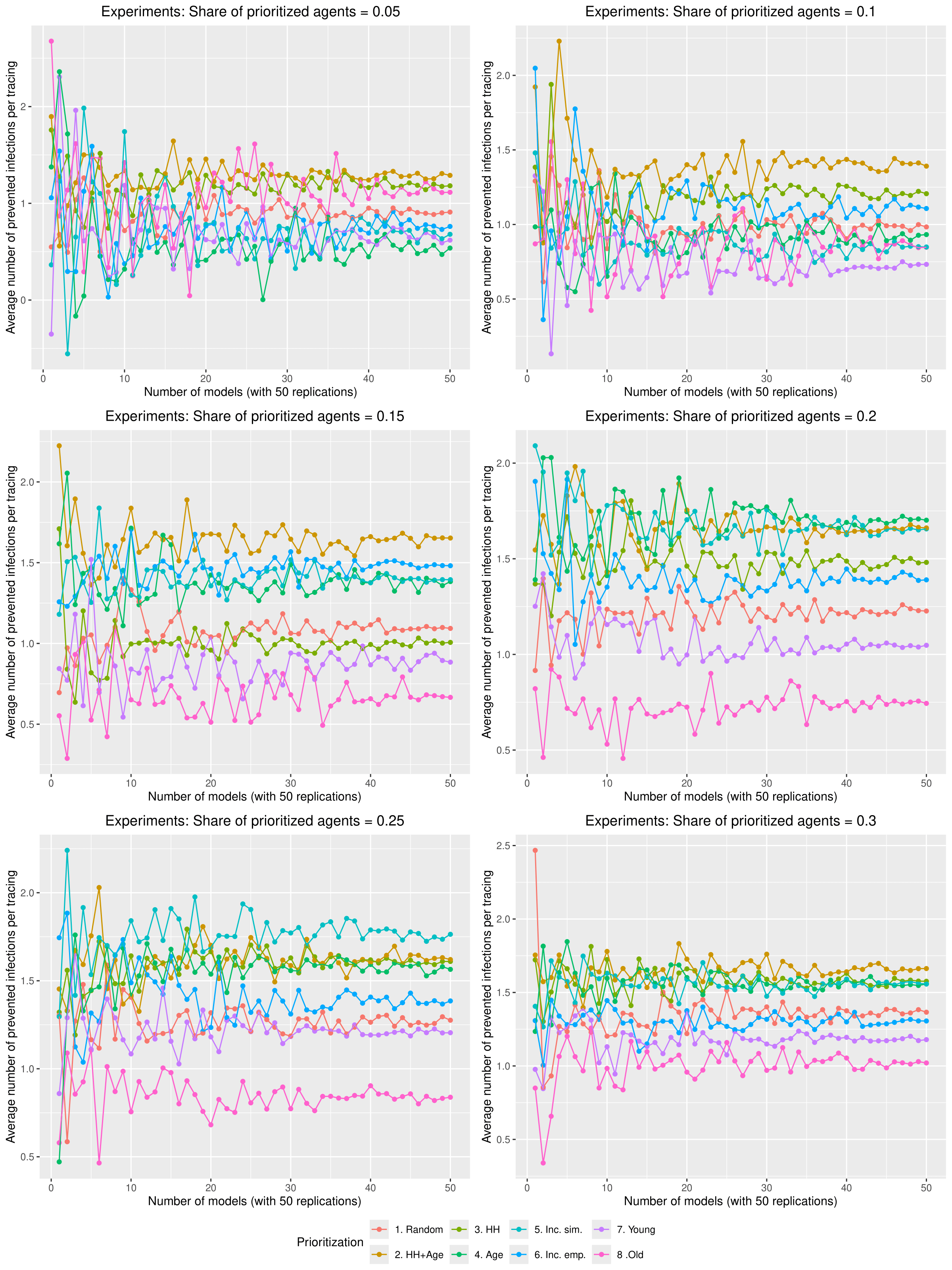
Figure 13 shows how the average number of prevented infections per tracing approaches a relatively stable state with 50 models in each scenario.
Appendix B: Results Regarding Hospitalizations
Appendix C: Sensitivity Analysis
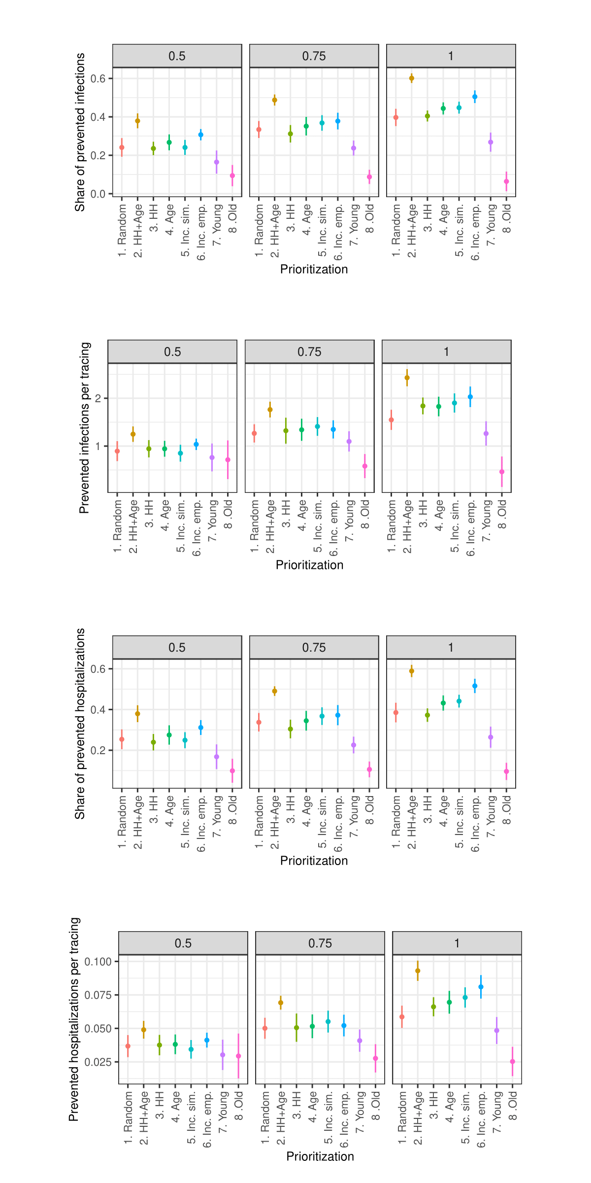
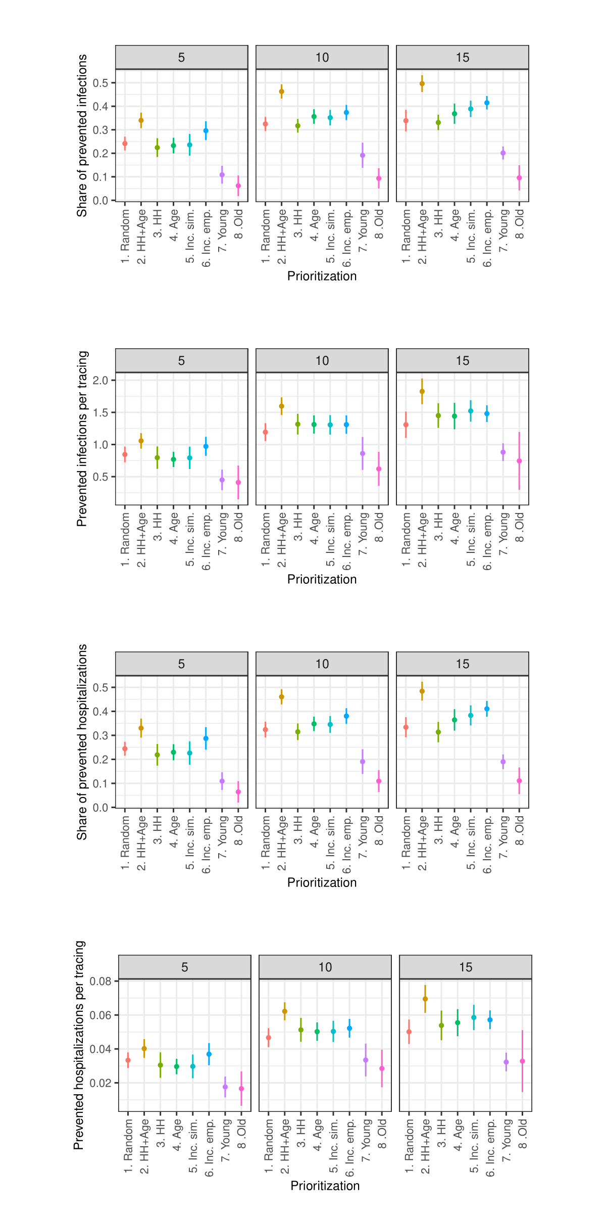
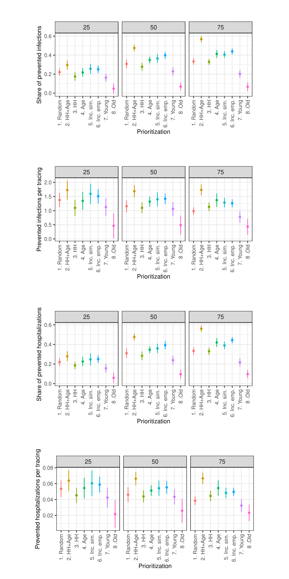
Due to constraints on available computational and storage capacity, the following sensitivity analysis is minimal. Only 25 models with 50 internal replications (1250 total) were performed per parameter combination and the share of prioritized agents was fixed to 0.15. Nevertheless, this section indicates that the general patterns in the results of the simulation experiments are relatively robust to parameter variations.
Sensitivity analysis: Contact tracing start date
Sensitivity analysis: Share of traced contacts
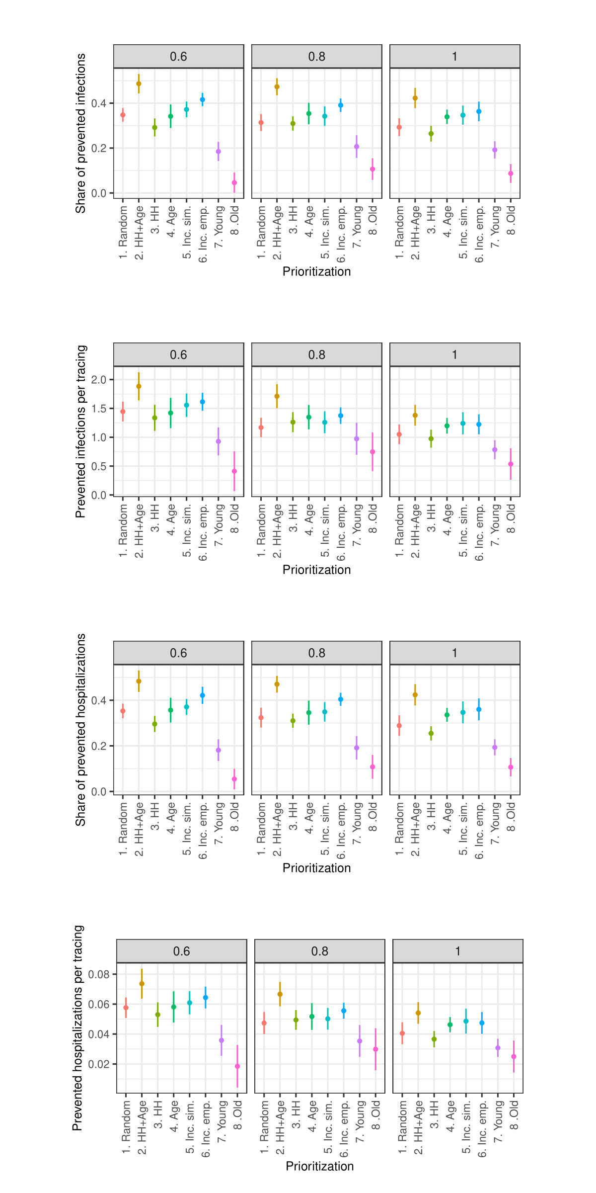
Sensitivity analysis: Isolation level within household
Sensitivity analysis: Days in quarantine
Sensitivity analysis: Maximum number of tracings per week
Sensitivity analysis: Change in infection probability
Sensitivity analysis: Days asymptomatic infectious
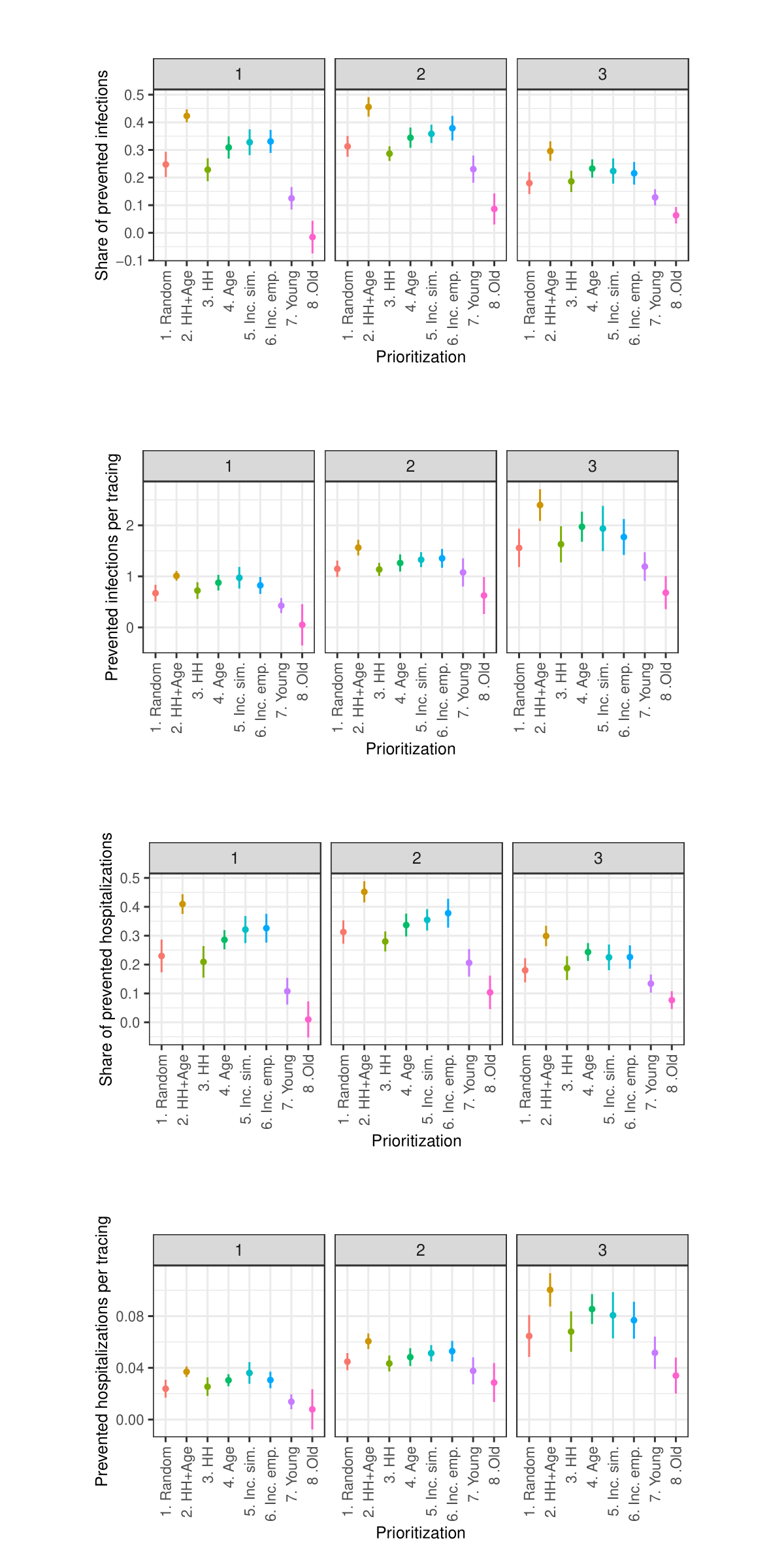
Sensitivity analysis: Length of simulated period
Notes
- For instance: degree centrality (Freeman 1978), betweenness centrality (Freeman 1977), eigenvector centrality (Borgatti 2005), closeness centrality (Sabidussi 1966), LeaderRank (Lü et al. 2011), bridging centrality (Hwang et al. 2006), H-index (Lü et al. 2016), and k-shell decomposition (Kitsak et al. 2010).↩︎
- The model’s code and data can be found in the corresponding repository on Github: https://github.com/simctbw/simctbw.↩︎
- From the perspective of the focus theory (Feld 1981), locations could also be regarded as foci.↩︎
- Thus, the defined location sizes are met not exactly by every location, but on average.↩︎
- We additionally considered values of 1 and 3 in the sensitivity analysis.↩︎
- To ensure that there is no systematic order within the group of agents having the same attribute value, we add a small random value to the attribute value.↩︎
- As the sensitivity analysis in the Appendix shows, we also tested values of 250 and 750 tracings per 100,000 agents per 7 days.↩︎
- As the sensitivity analysis in the Appendix shows, we also tested values of 50% and 100%.↩︎
- As the sensitivity analysis in the Appendix shows, we also tested values of 60% and 100%.↩︎
- Similar figures regarding prevented hospitalizations and prevented hospitalizations per tracing are presented in the Appendix.↩︎
- We define tracings as the number of agents that public health authorities must contact, i.e., both symptomatically ill agents whose contacts are traced and their contacts who are traced.↩︎
- Although the corresponding experiments are not reported in this paper, it should be noted here that this simulation model also replicates the findings that when it comes to vaccination, it is most effective to prioritize the oldest.↩︎
Appendix
References
AKIBA, T., Sano, S., Yanase, T., Ohta, T., & Koyama, M. (2019). Optuna: A next-generation hyperparameter optimization framework. Proceedings of the 25rd ACM SIGKDD International Conference on Knowledge Discovery and Data Mining.
ALIPOUR, J.-V., Falck, O., & Schüller, S. (2020). Germany’s capacities to work from home. European Economic Review, 151, 104354.
BANSAL, S., Pourbohloul, B., & Meyers, L. A. (2006). A comparative analysis of influenza vaccination programs. PLoS Medicine, 3(10), e387.
BEN-ZUK, N., Daon, Y., Sasson, A., Ben-Adi, D., Huppert, A., Nevo, D., & Obolski, U. (2022). Assessing COVID-19 vaccination strategies in varied demographics using an individual-based model. Frontiers in Public Health, 10.
BICHER, M., Rippinger, C., Urach, C., Brunmeir, D., Siebert, U., & Popper, N. (2021). Evaluation of contact-tracing policies against the spread of SARS-CoV-2 in Austria: An agent-based simulation. Medical Decision Making, 41(8), 1017–1032.
BORGATTI, S. P. (2005). Centrality and network flow. Social Networks, 27(1), 55–71.
BRADBURY‐JONES, C., & Isham, L. (2020). The pandemic paradox: The consequences of COVID-19 on domestic violence. Journal of Clinical Nursing, 29(13–14), 2047–2049.
BROOKS, S. K., Webster, R. K., Smith, L. E., Woodland, L., Wessely, S., Greenberg, N., & Rubin, G. J. (2020). The psychological impact of quarantine and how to reduce it: Rapid review of the evidence. The Lancet, 395(10227), 912–920.
BUBAR, K. M., Reinholt, K., Kissler, S. M., Lipsitch, M., Cobey, S., Grad, Y. H., & Larremore, D. B. (2021). Model-informed COVID-19 vaccine prioritization strategies by age and serostatus. Science, 371(6532), 916–921.
BUCKEE, C., Noor, A., & Sattenspiel, L. (2021). Thinking clearly about social aspects of infectious disease transmission. Nature, 595(7866), 205–213.
CARDOSO, M. R. A., Cousens, S. N., de Góes Siqueira, L. F., Alves, F. M., & D’Angelo, L. A. V. (2004). Crowding: Risk factor or protective factor for lower respiratory disease in young children? BMC Public Health, 4(1), 19.
COIBION, O., Gorodnichenko, Y., & Weber, M. (2020). Labor markets during the COVID-19 crisis: A preliminary view. National Bureau of Economic Research.
DESTATIS. (2022a). Kindertagesbetreuung: Betreuungsquote von Kindern unter 6 Jahren nach Bundesländern. https://www.destatis.de/DE/Themen/Gesellschaft-Umwelt/Soziales/Kindertagesbetreuung/Tabellen/betreuungsquote.html
DESTATIS. (2022b). Statistischer Bericht: Allgemeinbildende Schulen. Available at: https://www.destatis.de/DE/Themen/Gesellschaft-Umwelt/Bildung-Forschung-Kultur/Schulen/Publikationen/Downloads-Schulen/statistischer-bericht-allgemeinbildende-schulen-2110100227005.xlsx?__blob=publicationFile
DESTATIS. (2015). Zeitverwendungserhebung: Aktivitäten in Stunden und Minuten für ausgewählte Personengruppen.
DEZSŐ, Z., & Barabási, A.-L. (2002). Halting viruses in scale-free networks. Physical Review E, 65(5), 055103.
DODDS, W. (2019). Disease now and potential future pandemics. In W. Dodds (Ed.), The World’s Worst Problems (pp. 31–44). Cham: Springer International Publishing.
FDZ. (2022). Kinder und tätige Personen in Tageseinrichtungen und in öffentlich geförderter Kindertagespflege. Wiesbaden, Düsseldorf.
FELD, S. L. (1981). The focused organization of social ties. American Journal of Sociology, 86(5), 1015–1035.
FREEMAN, L. C. (1977). A set of measures of centrality based on betweenness. Sociometry, 40(1), 35–41.
FREEMAN, L. C. (1978). Centrality in social networks conceptual clarification. Social Networks, 1(3), 215–239.
FREYTAG, A., Link, E., & Baumann, E. (2021). "Selbst schuld!" - Stigmatisierung von COVID-19-Erkrankten und der Einfluss des individuellen Informationshandelns. Risiken und Potenziale in der Gesundheitskommunikation: Beiträge zur Jahrestagung der DGPuK-Fachgruppe Gesundheitskommunikation 2020.
GOEBEL, J., Grabka, M. M., Liebig, S., Kroh, M., Richter, D., Schröder, C., & Schupp, J. (2019). The German Socio-Economic Panel (SOEP). Jahrbücher Für Nationalökonomie Und Statistik, 239(2), 345–360.
HERRMANN, H. A., & Schwartz, J.-M. (2020). Why COVID-19 models should incorporate the network of social interactions. Physical Biology, 17(6), 065008.
HOEBEL, J., Grabka, M. M., Schröder, C., Haller, S., Neuhauser, H., Wachtler, B., Schaade, L., Liebig, S., Hövener, C., & Zinn, S. (2022). Socioeconomic position and SARS-CoV-2 infections: Seroepidemiological findings from a German nationwide dynamic cohort. Journal of Epidemiology and Community Health, 76(4), 350–353.
HWANG, W., Cho, Y.-r., Zhang, A., & Ramanathan, M. (2006). Bridging centrality: Identifying bridging nodes in scale-free networks. Available at: scispace.com/pdf/bridging-centrality-identifying-bridging-nodes-in-scale-free-r8j1phte2j.pdf
KAFFAI, M., & Heiberger, R. H. (2021). Modeling non-pharmaceutical interventions in the COVID-19 pandemic with survey-based simulations. PLoS One, 16, e0259108.
KEESING, F., Belden, L. K., Daszak, P., Dobson, A., Harvell, C. D., Holt, R. D., Hudson, P., Jolles, A., Jones, K. E., Mitchell, C. E., Myers, S. S., Bogich, T., & Ostfeld, R. S. (2010). Impacts of biodiversity on the emergence and transmission of infectious diseases. Nature, 468(7324), 647–652.
KERR, C. C., Stuart, R. M., Mistry, D., Abeysuriya, R. G., Rosenfeld, K., Hart, G. R., Núñez, R. C., Cohen, J. A., Selvaraj, P., Hagedorn, B., George, L., Jastrzębski, M., Izzo, A. S., Fowler, G., Palmer, A., Delport, D., Scott, N., Kelly, S. L., Bennette, C. S., … Klein, D. J. (2021). Covasim: An agent-based model of COVID-19 dynamics and interventions. PLoS Computational Biology, 17(7), e1009149.
KITSAK, M., Gallos, L. K., Havlin, S., Liljeros, F., Muchnik, L., Stanley, H. E., & Makse, H. A. (2010). Identification of influential spreaders in complex networks. Nature Physics, 6(11), 888–893.
KLÜSENER, S., Schneider, R., Rosenbaum-Feldbrügge, M., Dudel, C., Loichinger, E., Sander, N., Backhaus, A., Del Fava, E., Esins, J., Fischer, M., Grabenhenrich, L., Grigoriev, P., Grow, A., Hilton, J., Koller, B., Myrskylä, M., Scalone, F., Wolkewitz, M., Zagheni, E., & Resch, M. M. (2020). Forecasting intensive care unit demand during the COVID-19 pandemic: A spatial age-structured microsimulation model.
LIPPI, G., Henry, B. M., Bovo, C., & Sanchis-Gomar, F. (2020). Health risks and potential remedies during prolonged lockdowns for coronavirus disease 2019 (COVID-19). Diagnosis (Berlin, Germany), 7(2), 85–90.
LÜ, L., Zhang, Y.-C., Yeung, C. H., & Zhou, T. (2011). Leaders in social networks, the delicious case. PLoS One, 6(6), e21202.
LÜ, L., Zhou, T., Zhang, Q.-M., & Stanley, H. E. (2016). The H-index of a network node and its relation to degree and coreness. Nature Communications, 7(1), 10168.
MAHAJAN, A., Solanki, R., & Sivadas, N. (2021). Estimation of undetected symptomatic and asymptomatic cases of COVID‐19 infection and prediction of its spread in the USA. Journal of Medical Virology, 93(5), 3202–3210.
MANZO, G., & van de Rijt, A. (2020). Halting SARS-CoV-2 by targeting high-contact individuals. Journal of Artificial Societies and Social Simulation, 23(4), 10.
MARTIN, C. A., Jenkins, D. R., Minhas, J. S., Gray, L. J., Tang, J., Williams, C., Sze, S., Pan, D., Jones, W., Verma, R., Knapp, S., Major, R., Davies, M., Brunskill, N., Wiselka, M., Brightling, C., Khunti, K., Haldar, P., & Pareek, M. (2020). Socio-demographic heterogeneity in the prevalence of COVID-19 during lockdown is associated with ethnicity and household size: Results from an observational cohort study. EClinicalMedicine, 25, 100466.
MATRAJT, L., Eaton, J., Leung, T., & Brown, E. R. (2021). Vaccine optimization for COVID-19: Who to vaccinate first? Science Advances, 7(6), eabf1374.
MCPHERSON, M., Smith-Lovin, L., & Cook, J. M. (2001). Birds of a feather: Homophily in social networks. Annual Review of Sociology, 27, 415–444.
MISHRA, S., Steen, R., Gerbase, A., Lo, Y.-R., & Boily, M.-C. (2012). Impact of high-risk sex and focused interventions in heterosexual HIV epidemics: A systematic review of mathematical models. PLoS One, 7(11), e50691.
MOORE, S., Hill, E. M., Dyson, L., Tildesley, M. J., & Keeling, M. J. (2021). Modelling optimal vaccination strategy for SARS-CoV-2 in the UK. PLoS Computational Biology, 17(5), e1008849.
NAFILYAN, V., Islam, N., Ayoubkhani, D., Gilles, C., Katikireddi, S. V., Mathur, R., Summerfield, A., Tingay, K., Asaria, M., John, A., Goldblatt, P., Banerjee, A., Glickman, M., & Khunti, K. (2021). Ethnicity, household composition and COVID-19 mortality: A national linked data study. Journal of the Royal Society of Medicine, 114(4), 182–211.
NISHI, A., Dewey, G., Endo, A., Neman, S., Iwamoto, S. K., Ni, M. Y., Tsugawa, Y., Iosifidis, G., Smith, J. D., & Young, S. D. (2020). Network interventions for managing the COVID-19 pandemic and sustaining economy. Proceedings of the National Academy of Sciences, 117(48), 30285–30294.
NUNNER, H., van de Rijt, A., & Buskens, V. (2022). Prioritizing high-contact occupations raises effectiveness of vaccination campaigns. Scientific Reports, 12(1), 737.
PASTOR-SATORRAS, R., & Vespignani, A. (2002). Immunization of complex networks. Physical Review E, 65(3), 036104.
PELLIS, L., Ball, F., Bansal, S., Eames, K., House, T., Isham, V., & Trapman, P. (2015). Eight challenges for network epidemic models. Epidemics, 10, 58–62.
POLYAKOVA, M., Kocks, G., Udalova, V., & Finkelstein, A. (2020). Initial economic damage from the COVID-19 pandemic in the United States is more widespread across ages and geographies than initial mortality impacts. Proceedings of the National Academy of Sciences, 117(45), 27934–27939.
PREM, K., Cook, A. R., & Jit, M. (2017). Projecting social contact matrices in 152 countries using contact surveys and demographic data. PLoS Computational Biology, 13(9), e1005697.
ROBERT KOCH INSTITUT. (2025). 7-Tage-Inzidenz der COVID-19-Fälle in Deutschland. Available at: https://robert-koch-institut.github.io/COVID-19_7-Tage-Inzidenz_in_Deutschland/
SABIDUSSI, G. (1966). The centrality index of a graph. Psychometrika, 31(4), 581–603.
SAEED, F., Mihan, R., Mousavi, S. Z., Reniers, R. L., Bateni, F. S., Alikhani, R., & Mousavi, S. B. (2020). A narrative review of stigma related to infectious disease outbreaks: What can be learned in the face of the Covid-19 pandemic? Frontiers in Psychiatry, 11.
SHARMA, D., Bouchaud, J.-P., Gualdi, S., Tarzia, M., & Zamponi, F. (2021). V-, U-, L- or W-shaped economic recovery after Covid-19: Insights from an agent based model. PLoS One, 16(3), e0247823.
SOEP. (2021). Socio-Economic Panel (SOEP), data for years 1984-2019, version 36, SOEP, 2021.
STATISTISCHES Landesamt Baden-Württemberg. (2020). Bevölkerung Baden-Württembergs am 31. Dezember 2020 nach Alter und Geschlecht.
TRAD, F., & El Falou, S. (2022). Testing different COVID-19 vaccination strategies using an agent-based modeling approach. SN Computer Science, 3(4), 307.
VIERNICKEL, S., & Fuchs-Rechlin, K. (2015). Fachkraft-Kind-Relationen und Gruppengrößen in Kindertageseinrichtungen: Grundlagen, Analysen, Berechnungsmodell.
WACHTLER, B., Michalski, N., Nowossadeck, E., Diercke, M., Wahrendorf, M., Santos-Hövener, C., Lampert, T., & Hoebel, J. (2020). Socioeconomic inequalities and COVID-19 - A review of the current international literature.
WEI, X., Zhao, J., Liu, S., & Wang, Y. (2022). Identifying influential spreaders in complex networks for disease spread and control. Scientific Reports, 12(1), 5550.
WOOLHOUSE, M., Dye, C., Etard, J.-F., Smith, T., Charlwood, J., Garnett, G., Hagan, P., Hii, J., Ndhlovu, P., Quinnell, R., Watts, C., Chandiwana, S., & Anderson, R. (1997). Heterogeneities in the transmission of infectious agents: Implications for the design of control programs. Proceedings of the National Academy of Sciences, 94(1), 338–342.
ZHU, J., & Wang, L. (2021). Identifying influential nodes in complex networks based on node itself and neighbor layer information. Symmetry, 13(9), 1570.