Stratified Configuration Model for Simulating Networks

Introduction

Complex networks are models used to study relationships between pairs of elements, called nodes. Applications are closely related to the set of nodes under analysis. The Internet, for instance, is a network where the set of nodes is made up of computers joined by data connections. The World Wide Web is a network where the set of nodes is made up of web pages and links between them. In a network of physical contacts, the set of nodes is made up of people whose relationships are based on the physical contact they have had over a specific period of time.

The study of complex networks focuses on the analysis of the connection pattern among the nodes. In general, the set of relationships does not exhibit a straightforward structure, as is the case when every pair of nodes is connected, nor does it resemble randomly established connections. Given the intricacy of their connection patterns, real networks are often characterized by a wide range of parameters that describe several of their properties, such as clustering, degree, assortativity, and diameter, among others (Newman 2018). Many applications require generation models that produce networks with some given values of those parameters.

For that task, it is common to resort to generating graph models – such as Erdös-Rényi (ER) (Erdős & Rényi 1959), Barabási-Albert (BA) (Barabási & Albert 1999) and the Configuration Model (CM) (Newman 2018). However, a limitation shared by many models, including the configuration model, is that they do not consider neither the attributes of the components or nodes nor the properties of links in the construction of networks.

Factors such as age, gender, knowledge, disease pre-disposition and social-economic level influence the network of contacts of an individual. For example, Christakis & Fowler (2007) in their study of hospital networks, demonstrate that individuals with obesity are more likely to form connections with others who are also obese, rather than with those who are not. Bhattacharya et al. (2008) show that, in trade networks, wealthy countries are much more strongly connected. This is known as homophily in the study of complex networks (McPherson et al. 2001). The relevance of node attributes in network connections goes beyond the simple homophily vs. heterophily dichotomy (Kim & Altmann 2017). As an example, Mossong et al. (2008) show a decrease in the number of interpersonal contacts as age increases. All in all, real-world networks exhibit a complex interrelation between their topology and node attributes that cannot be replicated by the state-of-the-art graph generating algorithms.

To address this limitation, this article proposes an extension of the CM, called the Stratified Configuration Model (STCM). Indeed, whereas the Configuration Model, described in some detail later in this work, is effective in creating a network of nodes with a pre-specified number of connections for each of them, it cannot account for the node properties. The STCM, on the contrary, splits the nodes into different categories (strata), capturing nodes’ attributes, and accounts for the probabilities of attribute-dependent connections. The proposed STCM framework introduces three key advantages. Firstly, it incorporates a tunable parameter that explicitly governs the network’s clustering coefficient, allowing the generation of topologies with a higher density of local structures often observed in empirical systems. Secondly, the model demonstrates remarkable consistency in reproducing the prescribed inter-strata connectivity patterns, a property that remains robust even as the network size and overall clustering increase. Finally, and perhaps most significantly, the underlying algorithm can construct these globally coherent networks based on local rules, without requiring complete topological information, which underscores its efficiency and scalability for modelling large-scale systems. In summary, STCM is a generative model designed to produce realistic networks, even in certain missing-data situations. Indeed, it was used for that purpose in Gonçalves et al. (2026). Nonetheless, it could also be used as a reference model that extends the well-known configuration model to account for node attributes, explicitly considering node weights and how they alter the resulting linking patterns.

The remaining of the article is organized as follows. First, we review recent models that incorporate node attributes in network construction and discuss the main differences compared to our algorithm. Then we detail the proposed algorithm along with its two variations. We evaluate the performance of the generating model through experiments based on two different datasets and compare the results with three state-of-the-art models, discussing the findings obtained. Finally, we highlight the study’s key findings and discuss the model’s limitations and potential extensions.

State-of-the-Art Network Generation Models

As discussed earlier, complex networks can exhibit several peculiar characteristics that we wish to replicate in reference models. In this context, Drobyshevskiy & Turdakov (2019) classify network generation models in three broad families: Generative, Feature-driven, and Domain-specific. The Generative class encompasses all graph generation mechanisms designed to qualitatively explain observed connection patterns, where the model’s development is carried out by constructing the graph from predefined rules, identifying its characteristics, and then comparing them with real patterns to adjust the rules as necessary. In contrast, the Feature-driven class focuses on creating models that quantitatively fit sets of desired characteristics; that is, from a pre-established set of attributes, one seeks to develop or refine a model that exactly meets such requirements. Finally, the Domain-specific class concerns graph generation methods that incorporate additional network attributes, such as community structure or edge weights, meeting specific requirements of certain application domains. In this work, the focus is on Generative and Feature-driven models.

Traditional graph formation models are of the Generative type. The simplest model to be analysed is the random graph model presented by Erdős & Rényi (1959), in which the connection between any two nodes \(i\) and \(j\) occurs with a fixed probability \(p\). One of the main advantages of the ER model is its simplicity, combined with the availability of numerous analytical results regarding network behaviour. However, this model neither incorporates structural characteristics nor does it account for attributes of the nodes or edges.

With the advancement of studies on networks in different contexts, structural patterns such as scale-free networks (Abe & Suzuki 2004; Albert 2005) and small-world networks (Bassett & Bullmore 2006; Latora & Marchiori 2002) were identified. To replicate such properties, reference models were developed, such as the Barabási-Albert model (Barabási & Albert 1999), which describes networks whose degrees follow a power-law distribution, and the Watts-Strogatz model (Watts & Strogatz 1998), which combines high transitivity with short characteristic path lengths.

Another recurring problem is faithfully reproducing the desired degree distribution so that each node maintains the number of connections predicted theoretically. To address this issue, the Configuration Model (CM) (Newman 2018) initially distributes "stubs" to the nodes based on their desired degrees, connecting them randomly until the entire network is formed. This approach preserves the expected degree distribution. Moreover, its analytical study is straightforward and serves as basis in the study of networks characteristics which are strictly related to the degree distribution. However, a limitation of the Configuration Model is that the resulting network’s clustering coefficient is very small (Newman 2018).

An assumption of the configuration model is that it must exactly reproduce the degree of each node; however, this is unrealistic, as in most applications the collected data contain noise. To relax this constraint, the Soft Configuration Model (SCM) was proposed (Bianconi 2007; Park & Newman 2004; van der Hoorn et al. 2017). It relaxes the constraint from a fixed degree sequence to a fixed expected degree sequence. The SCM is a canonical ensemble that maximizes Gibbs entropy, where the probability of an edge between nodes \(u\) and \(v\) is given by \(p_{uv} = (e^{\lambda_u + \lambda_v} + 1)^{-1}\). In this formulation, the Lagrange multipliers \(\lambda_u\) are uniquely determined to satisfy the constraint \(\langle k_u \rangle = \sum_{\nu \ne u} p_{u\nu}\) for each node \(u\), where \(\langle k_u \rangle\) is its expected degree. This approach is more robust to the noise and stochasticity inherent in real-world network data, as it does not enforce an exact degree for each node in every realization. The main novelty of the SCM is thus the transition from a microcanonical to a canonical ensemble, allowing the degree of each node to fluctuate around its expected value, thereby introducing an additional source of randomness.

The Chung-Lu model (Chung & Lu 2002b, 2002a) represents a framework for generating random networks conditioned on a prescribed expected degree sequence. In this model, each vertex \(u\) is assigned a weight \(w_u\), corresponding to its expected degree in the resulting network. The core theoretical foundation lies in defining the edge probability between vertices \(u\) and \(v\) as the product of their weights, scaled by the aggregate sum of all weights in the network. Formally, the connection probability is expressed as:

\[p_{uv} = \min\left\{1, \frac{w_u w_v}{\sum_\nu w_\nu}\right\}\]

\[(1)\]

where the minimization ensures \(p_{uv} \leq 1\), circumventing inadmissible probabilities in sparse regimes. Crucially, this formulation guarantees that the expected degree of vertex \(u\) equals \(w_u\) under the model’s constraints.

From an implementation perspective, network construction proceeds stochastically: for each vertex pair \((u,v)\), an edge is generated independently with probability \(p_{uv}\). This Bernoulli sampling mechanism ensures edge independence — a defining property that distinguishes the Chung-Lu model from configuration-based approaches. Notably, the model achieves exact correspondence between prescribed weights \(\{w_\nu\}\) and expected degrees without requiring iterative adjustments, offering computational advantages in large-scale simulations. Moreover, the independence of edge formations facilitates analytical tractability, making the model particularly amenable to theoretical derivations of network properties.

Thus far, the models presented do not incorporate non-structural characteristics of nodes into their formulation. To address this gap, a widely discussed family of models in the literature are the so-called Exponential Random Graph Models (ERGMs) (Chatterjee & Diaconis 2013; Frank & Strauss 1986; Robins et al. 2007). Following Chatterjee & Diaconis (2013), let \(\mathcal{G}_N\) be the set of all graphs with \(N\) nodes (e.g., if we consider all undirected graphs with no loops and no multiple edges, \(|\mathcal{G}_N| = 2^{N(N-1)/2}\)). Then, for each \(G\in\mathcal{G}_N\), its probability is given by:

\[P(G) = \frac{1}{Z} \exp \Biggl( \sum_\alpha \eta_\alpha \cdot g_\alpha(G) \Biggr), \]

\[(2)\]

where \(g_\alpha(G)\) are real-valued functions on \(\mathcal{G}_N\) which represent network characteristics (e.g., average degree), \(\eta_\alpha\) are the coefficients that weight each characteristic, reflecting the logarithmic variation of the unitary increment in their respective statistic, and \(Z\) is the normalization constant. The key advantage of this model lies in its probabilistic rigour, which is grounded in the Maximum Entropy principle. The resulting distribution of networks is the one that maximizes entropy subject to a given set of constraints (specified by the parameters \(\eta_\alpha\)), meaning the model assumes no further information beyond these constraints. To estimate the parameters \(\eta_\alpha\) that best explain the observed network properties \(g_\alpha(G)\), various methods can be employed, such as Maximum Likelihood (Besag 1986; Handcock 2003), Maximum Pseudo-Likelihood (Strauss & Ikeda 1990), and Markov Chain Monte Carlo (MCMC) (Geyer & Thompson 1992; Goodreau 2007; Snijders 2002). However, as more network properties are included, the model becomes progressively more complex, the convergence of the estimation algorithms tends to be slower (especially when the number of nodes exceeds \(10^4\)) (He & Zheng 2013), and there is no guarantee that the estimation process will reach the global optimum.

There are simplifications of the ERGM that seek to incorporate node attributes more efficiently. For example, the Stochastic Block Model (SBM) (Lee & Wilkinson 2019) was introduced as a simple way of utilizing additional attributes in the nodes. In the SBM, each node is classified into a block \(B \in \{0,1,2,\dots,N\}\), representing a categorical attribute. The probability of connection between two nodes belonging to blocks \(k\) and \(l\) is given by \(p_{kl}\), resembling the Erdős–Rényi model. However, this approach, like ER, does not faithfully reproduce more complex degree distributions, limiting its ability to describe networks that exhibit greater structural heterogeneity. This limitation is directly addressed by the Degree-Corrected Stochastic Block Model (DCSBM) and its generalizations (Karrer & Newman 2011; Peixoto 2014, 2019). The primary shortcoming of the traditional SBM stems from its foundational premise of stochastic equivalence, which posits that all nodes within a given block are statistically indistinguishable. This imposes the stringent constraint that the expected degree is uniform for all members of a block, a condition fundamentally at odds with the heterogeneity observed in empirical networks. DCSBM alleviates this by introducing a node-specific parameter, \(\theta_\nu\), which controls the expected degree of node \(\nu\). This modification effectively decouples a node’s intrinsic connectivity (its degree) from its community affiliation, allowing for the inference of mesoscale structures that are not confounded by degree heterogeneity.

In particular, DCSBM assumes that the number of edges, \(\mathbf{A}_{u,v}\), between nodes \(u\) and \(v\) is a realization of a Poisson random variable with expected value \(\lambda_{u,v} = \theta_u \theta_v \mathbf{\Omega}_{f_u,f_v}\), where \(\mathbf{\Omega}_{f_u,f_v}\) is a parameter that accounts for the propensity of connections between groups \(f_u\) and \(f_v\) to which nodes \(u\) and \(v\) belong, respectively. As a generative model, DCSBM provides a straightforward procedure for synthesizing networks. Given a set of parameters—group assignments \(\{f_\nu\}\), degree propensities \(\{\theta_\nu\}\), and an affinity matrix \(\mathbf{\Omega}\)—a network is constructed by independently drawing \(\mathbf{A}_{u,v} \sim \text{Poisson}(\lambda_{u,v})\) for each node pair. From an inferential standpoint, given a completely observed network with known group assignments, the model’s parameters are estimated by maximizing the log-likelihood function, obtaining (see Karrer & Newman 2011):

\[\begin{aligned} \hat{\theta}_u = \frac{k_u}{\sum\limits_{\nu} k_\nu\delta_{f_\nu,f_u}},\qquad \hat{\mathbf{\Omega}}_{a,b} = \sum\limits_{u,v} \mathbf{A}_{u,v}\delta_{f_u,a}\delta_{f_v,b};\end{aligned}\]

\[(3)\]

i.e., \(\hat{\theta}_u\) is the fraction of edges connecting group \(f_u\) that corresponds to node \(u\), and \(\hat{\mathbf{\Omega}}_{a,b}\) is the number of edges that connect groups \(a\) and \(b\). If group assignments are unknown, there are different strategies that can be followed. Since we are not interested in that case here, we refer the interested reader to the relevant literature (Karrer & Newman 2011; Peixoto 2014, 2019).

Despite its significant advantages, DCSBM possesses several intrinsic limitations. First, the Poisson assumption, while mathematically convenient, naturally generates multi-graphs and may not be appropriate for strictly simple graphs, while also fixing the variance of edge counts to their mean. Second, the model’s premise of conditionally independent edges prevents it from capturing higher-order network structures. Notably, it fails to explicitly model triadic closure, often resulting in generated networks with significantly lower clustering coefficients than their empirical counterparts. Finally, the number of degree parameters, \(\{\theta_\nu\}\), scales linearly with the number of nodes, \(N\) (Karrer & Newman 2011). This makes the model inherently transductive and complicates the task of generalizing a fitted model to generate larger networks. Indeed, if one takes a given network \(G_1\) with \(N_1\) nodes and estimates the parameters \(\{\theta_\nu\}_{\nu=1}^{N_1}\) as explained, those values cannot be easily generalized for the generation of an ‘equivalent’ network \(G_2\) with \(N_2\) nodes. One possibility would be to sample a set \(\{\theta'_\mu\}_{\mu=1}^{N_2}\) from \(\{\theta_\nu\}_{\nu=1}^{N_1}\) with an adequately chosen distribution or, in the case that \(N_2 = r\times N_1\) with \(r\in\mathbb{N}\), to make \(r\) copies of the original set. However, these adaptations are not part of the original DCSBM and our proposal provides solutions for the problem of changing the network size. Moreover, DCSBM and its generalizations do not deal with partially observed networks as we do in this work.

SBM and DCSBM impose strong assumptions, notably the probabilistic independence of edges and the preservation of the total number of edges \(m\) only in expectation, typically under a Poisson distribution. Such assumptions are frequently violated in empirical systems, where interactions are correlated and the total number of connections is a fixed, observed value, not a random variable. These limitations compromise both the accuracy of the fit and the conceptual validity of the model in resource-constrained contexts.

The Generalized Hypergeometric Ensemble of Random Graphs (gHypEG) proposes an elegant solution to these difficulties by reformulating the configuration model as an urn problem (Casiraghi et al. 2016; Casiraghi 2019; Casiraghi & Nanumyan 2021). This innovative approach yields a closed-form probability distribution – the multivariate hypergeometric distribution – which, crucially, conditions the graph ensemble on an exact number of edges \(m\). By doing so, gHypEG relaxes the premise of edge independence and positions itself as a robust intermediate alternative between the canonical configuration model, which preserves degrees exactly but is computationally intractable, and models like the Chung-Lu model (Chung & Lu 2002a), which preserve degrees and edges only in expectation. The hypergeometric configuration model departs from an urn model approach to sampling edges. Indeed, if \(k_\nu^{in}\) and \(k_\nu^{out}\) are the input and output degrees of node \(\nu\), respectively, there are \(\mathbf{\Xi}_{u,v}=k_u^{out}k_v^{in}\) possible edges between nodes \(u\) and \(v\). From the multiset of \(\sum_{u,v} \mathbf{\Xi}_{u,v}\) edges, a fixed number \(m\) of links are sampled without replacement. A preferential attachment between two nodes \(u\) and \(v\), dependent on other properties or characteristics, can be accomplished by using a biased sampling. For that purpose, Casiraghi and colleagues introduced a propensity matrix \(\mathbf{\Omega}\) such that the odds-ratio of an edge between \(u\) and \(v\) and one between nodes \(w\) and \(x\) is given by \(\mathbf{\Omega}_{u,v}/\mathbf{\Omega}_{w,x}\). This mechanism of biased sampling from an urn can be described by the Wallenius’ noncentral hypergeometric distribution, thus facilitating the mathematical analysis of the generated networks and the estimation of parameters from a given set of graphs. Block structure can be introduced in gHypEG by using a block-structured matrix \(\mathbf{\Omega}\), that is, a matrix with elements that depend only on the groups of the source and destination nodes. We shall denote the resulting model as Block-Constrained Generalized Hypergeometric Model.

As we shall explain, our proposal for network generation differs from that of Casiraghi and colleagues as we proceed in a manner closer to the original configuration model. Indeed, we first assign \(k_\nu^{in}\) input and \(k_\nu^{out}\) output stubs to each node \(\nu\). Then, we distribute each of those stubs to connections with nodes of different groups following multinomial distributions based, not on the propensities, but on actual probabilities of connections between groups. We shall compare both the STCM and gHypEG for network generation later in the paper. As for the estimation of parameters, let us also note that the generalized hypergeometric model requires complete knowledge of the graph, while our approach deals with the case of partial knowledge.

The Kronecker Graph model (Leskovec et al. 2010), leverages the self-similarity property generated by the Kronecker product to model large-scale networks. In its deterministic form (KGM), the adjacency matrix \(\mathbf{K}_k\) of a large graph is obtained by the \(k\)-th Kronecker power of the adjacency matrix \(\mathbf{K}_1\) of a small initiator graph (\(N_1 \times N_1\)), thereby replicating the structure of \(\mathbf{K}_1\) recursively and generating a graph with \(N=N_1^k\) nodes.

The stochastic extension (SKGM), which is the primary focus for modelling real-world data and parameter estimation, replaces the binary initiator matrix \(\mathbf{K}_1\) with a probability matrix \(\mathbf{\Theta}_1\) (also of dimension \(N_1 \times N_1\)). The \(k\)-th Kronecker power of this matrix, \(\mathbf{P}_k = \mathbf{\Theta}_1^{[k]}\), is not directly the adjacency matrix but rather an \(N \times N\) matrix (with \(N=N_1^k\)) where each entry \(p_{uv}\) defines the probability of an edge existing between nodes \(u\) and \(v\). To obtain a specific graph (a realization), each potential edge \((u,v)\) is included independently with probability \(p_{uv}\). The probability \(p_{uv}\) is calculated by the product of the corresponding entries of \(\mathbf{\Theta}_1\) along the recursive structure. Specifically, if the indices \(u, v\) (from \(1\) to \(N_1^k\)) are represented in base \(N_1\) by the digits \(u_{k-1}, \dots, u_0\) and \(v_{k-1}, \dots, v_0\), then:

\[p_{uv} = \prod_{i=0}^{k-1} \mathbf{\Theta}_1[u_i+1,\, v_i+1]\]

\[(4)\]

This mechanism generates a graph where connections are formed probabilistically, yet the probability structure \(\mathbf{P}_k\) itself exhibits a self-similar nature, inherited from the initiator matrix \(\mathbf{\Theta}_1\). A useful interpretation of the parameters \(\theta_{ij}\) in \(\mathbf{\Theta}_1\) is to associate them with affinities between implicit node categories or attributes at each recursive level; high values on the diagonal \((\theta_{ii})\) indicate a higher probability of connection between nodes sharing the same category at that level (homophily), while off-diagonal values \((\theta_{ij}, i \neq j)\) model the probability of connections between nodes of distinct categories (heterophily).

Despite its strengths in capturing global network properties and scalability, the Kronecker Graph model has limitations. A primary constraint is the structural requirement that the number of nodes \(N\) must be an integer power of the initiator matrix size \(N_1\) (i.e., \(N=N_1^k\)). Fitting the model to real networks often necessitates padding the graph with isolated nodes to meet this requirement, which might subtly affect parameter estimation, although empirically this effect seems manageable. Furthermore, while the SKGM effectively models many global statistics like degree distributions and diameters, it may not perfectly replicate all aspects of local structure, such as specific clustering patterns or community motifs beyond the recursive self-similarity imposed by the Kronecker product. The interpretation of associating \(\mathbf{\Theta}_1\) entries with simple attribute affinities might also oversimplify the complex mechanisms driving link formation in real-world networks. Finally, the likelihood function for parameter estimation is non-convex, presenting potential optimization challenges, although algorithms like KronFit (Leskovec et al. 2010) have proven empirically robust.

Although many studies consider node weights in a categorical manner, there are also works that address continuous values. For instance, Oliveira et al. (2022) propose a model aimed at studying geographic networks, highlighting their relevance in the context of statistical physics. In this model, the addition of a new node to the network follows a probabilistic dynamic: for each pre-existing node, the formation of an edge is governed by a probability that decreases according to a power-law distribution as a function of the distance between nodes.

Turning to the structure of connections itself, multi-layer networks emerge as essential mathematical structures for describing complex systems with multiple layers of interaction, allowing the representation of different types of relationships (e.g., social, technological, biological) among the same elements within an integrated structure. This approach is particularly relevant, as it captures the diversity of real-world interactions more comprehensively than traditional single-layer networks, enabling more precise analyses of dynamic phenomena. In this context, Zhou & Zhou (2018) propose a general model for generating multiplex networks, starting from the merger of two simple networks with an equal number of nodes and simultaneously controlling the degree distribution of each layer, intra- and inter-layer degree correlations, and edge overlap, using a probabilistic algorithm to satisfy the desired specifications. Conversely, focusing on empirical applications such as public health, Klise et al. (2022) present a methodology that generates subnetworks by age stratum, groups individuals into family structures (household cliques) based on census data, and adjusts social interactions according to mobility and vulnerability patterns, creating realistic networks to simulate intervention strategies, such as COVID-19 vaccination. In the remaining of this paper, we focus on single layer networks.

In summary, traditional network models commonly neglect nodal attributes, whereas more recent approaches attempt to incorporate them. However, some of these newer models suffer from low interpretability or are computationally expensive. SBM-based models emerge as a statistically grounded solution to this problem, but they rely on strong assumptions such as Poisson degree distributions and edge independence, and they tend to produce networks with low clustering.

In this study, we introduce a model designed to effectively replicate diverse patterns of internal connectivity in networks characterized by categorical node attributes, aiming for a balance between generality and computational efficiency. Our model is capable of generating networks with high clustering coefficients, accurately reproducing the observed interconnection patterns between categories. Unlike SBM-based models, it does not assume edge independence, adheres strictly to the empirical degree distribution of the input dataset, and allows for heterogeneous degree distributions across different node categories.

Stratified Configuration Model

In this scenario, we propose an extension of the Configuration Model which incorporates additional information about the node categories. To this end, we first consider an undirected graph \(G=(\mathcal{N},\mathcal{E})\) with \(\mathcal{N} = \{\nu_1,\nu_2,\cdots,\nu_N\}\) the set of nodes and \(\mathcal{E}\subseteq \mathcal{N}\times \mathcal{N}\) the set of edges. While this foundational definition assumes an undirected structure (i.e., \((u,v) \in \mathcal{E} \iff (v,u) \in \mathcal{E}\)), we will later extend the framework to accommodate directed graphs. In what follows, we assume that there are no self-loops in \(G\), i.e., \((\nu,\nu)\not\in \mathcal{E}\) for any \(\nu\in\mathcal{N}\). In our problem, each node belongs to one and only one category from a discrete set \(\mathcal{F}\) and the distribution \(F\) determines the frequency of each category in the network. For the sake of clarity, we shall call \(f_\nu\) the category to which node \(\nu\) belongs. Let us assume that the degree distribution depends on the category so that we can write \(K(f)\) for this distribution for a category \(f\in\mathcal{F}\). The average frequency of connections between two categories \(f\) and \(a\) is given by the element \({\mathbf{M}}_{f,a}\) of a matrix \({\mathbf{M}}\). We shall assume that \(\mathcal{F}\), \(F\), \(K(f)\) for all \(f\in\mathcal{F}\), and \({\mathbf{M}}\) are known or can be estimated from empirical data.

Network generation begins by creating a set of nodes \(\mathcal{N}\) with size \(N\). For each node \(\nu\in\mathcal{N}\), we assign a category \(f_\nu\) drawn from the distribution \(F\). Then, the total number of neighbours of that node, \(k_\nu\), is chosen using the distribution \(K(f_\nu)\). The number of edges that node \(\nu\) establishes with nodes of each category \(f\), \(\kappa_{\nu,f}\) \(\forall f\in\mathcal{F}\), is drawn from a multinomial distribution with total number \(k_\nu\) and probabilities \({\mathbf{M}}_{f_\nu,:}\) (i.e., \(\mathbf{Multi}(k(\nu_f),\mathbf{M}_{f_\nu,:})\)). Finally, the Configuration Model is applied to this structure. Nodes are processed in descending order of degree in order to increase the algorithm convergence speed (Manzo & van de Rijt 2020). The resulting network accounts for both the degree distribution of the nodes within each category and the connection affinity between categories. This reformulation of the CM will be referred to as the Stratified Configuration Model.

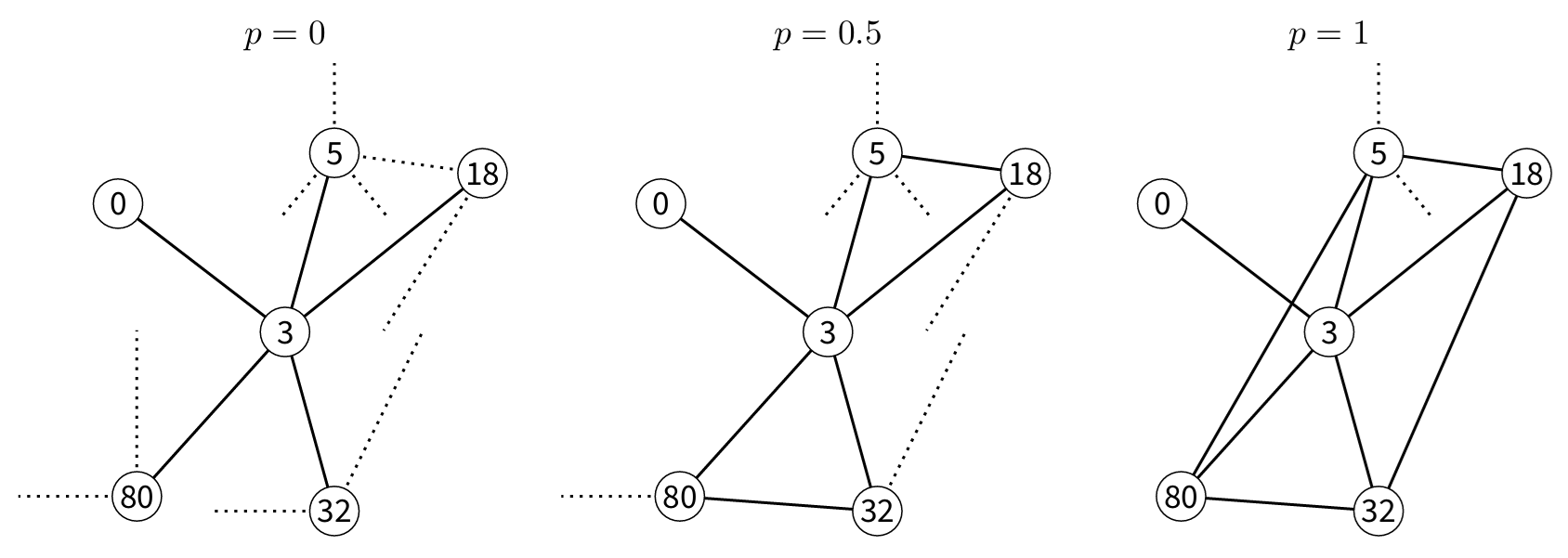
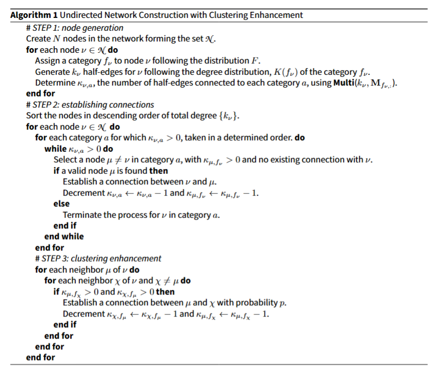
The STCM inherits from the CM the limitation of producing low clustering coefficient values. To overcome this problem, Manzo & van de Rijt (2020) propose an algorithm that increases the network’s clustering coefficient (see Figure 1). In general, when a vertex reaches its target degree or can no longer be connected to other nodes due to restrictions imposed by its neighbours (or successors), a new step is introduced: each pair of neighbours is connected with a probability \(p\). This strategy increases the likelihood of triangle formation, thereby enhancing the final clustering coefficient. Algorithm 1 presents the pseudocode of the STCM with the approach of Manzo & van de Rijt (2020).

It must be noted that there is no guarantee that all of the stubs or half-edges assigned to each node at the beginning of the algorithm will be connected. This fact is a result of choosing the values \(\kappa_{\nu,\cdot}\) for each node \(\nu\) independently. The consequence is a ‘loss’ in the total number of edges. Fortunately, as it will be shown later in this paper, the proportion of lost edges in real-world cases is small.

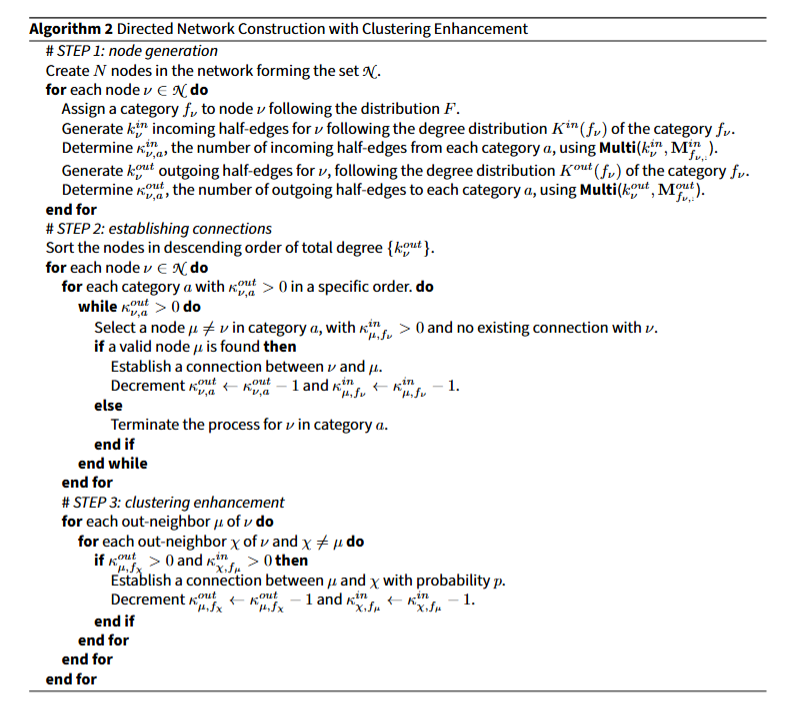
The Stratified Configuration Model can be extended to directed networks. For that purpose, it is necessary to consider two distinct distributions: \(K^{in}(f_\nu)\), which describes incoming connections, and \(K^{out}(f_\nu)\), which describes outgoing connections, as well as two matrices, \(\mathbf{M}^{in}_{f,a}\) and \(\mathbf{M}^{out}_{f,a}\), responsible for generating \(\kappa^{in}_{\nu,a}\) and \(\kappa^{out}_{\nu,a}\), respectively. Algorithm 2 presents the pseudocode for the directed STCM.

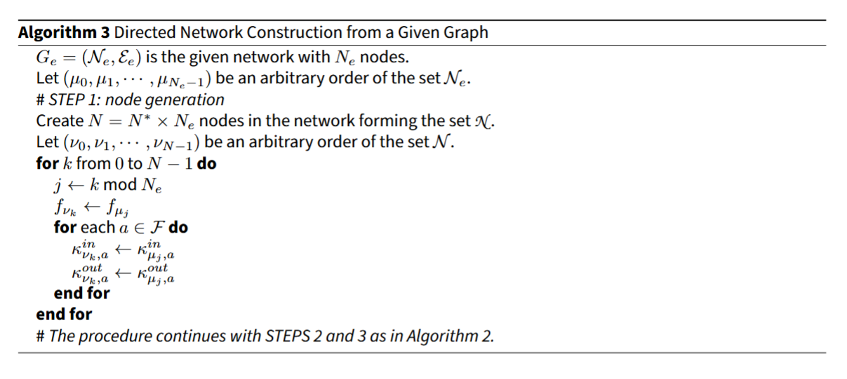
So far, we have assumed that network parameters such as \(F\), \(K(f)\) and \(\mathbf{M}\) are either known or estimated from empirical data, e.g., a set of surveyed graphs. However, in occasions we have access to a single network which is completely known and we need to artificially generate new graphs with similar characteristics. Under this setting, we can extract the values of \(\kappa_{\nu,a}\) and the category \(f_\nu\) for each node \(\nu\) directly from the original graph and, essentially, proceed as in Algorithm 1. Proceeding that way, we can generate a network with the same number of nodes as the original one. If larger networks with a similar structure are desired, we can proceed by first making several copies of the empirically known graph (in this sense, the construction resembles that of the Kronecker model). Algorithm 3 presents the details of the resulting procedure (for the sake of simplicity, only the directed case is presented).

Evaluation of the Proposed Generating Model

The evaluation of the STCM model involves its comparison with real-world networks and the analysis of its behaviour as a function of network size (scalability) and clustering properties. To this end, we utilized two datasets corresponding to two different application cases. Indeed, it is often the case that only some statistics of the network are known, but its complete structure is ignored. In those situations, it is useful to create artificial networks which are compatible with the given statistics using, e.g., Algorithm 1. Below, we use the Stratified Configuration Model with incomplete data on interpersonal contacts from the POLYMOD survey (Mossong et al. 2008). In other situations, the exemplary network (or a small part of it) is known in its entirety. The problem, then, is to create similar (but different) networks, sometimes larger than that known, using Algorithm 3. For the analysis of this case, we resort to a well-known network of political blogs (Adamic & Glance 2005). Furthermore, to comprehensively assess the performance of the proposed approach, the STCM model is compared against DCSBM and gHypEG. DCSBM was selected as it represents the established standard for integrating block structure with degree heterogeneity in community-structured networks, despite its limitations regarding edge independence and Poisson-distributed edge counts. gHypEG, in turn, represents a recent advancement that addresses these specific shortcomings by conditioning the graph ensemble on an exact number of edges through the multivariate hypergeometric distribution. Comparing STCM against both models allows us to evaluate its performance relative to a widely adopted benchmark and a state-of-the-art approach that shares the property of exactly preserving edge counts. However, we can only make the comparison in the case of the network of political blogs as it is completely known. Indeed, both DCSBM and gHypEG require complete knowledge of the graph in order to estimate the parameters.

Incomplete knowledge of the network: The POLYMOD case

Data

Aiming to study the influenza pandemic, the European Commission launched a project called POLYMOD, designed to collect data to understand the patterns of social contacts across Europe (Mossong et al. 2008). Based on this study, subsequent research was inspired by the POLYMOD framework (Mossong et al. 2017). This research was conducted using a survey between May 2005 and September 2006 in eight different European countries, utilizing random phone calls or face-to-face interviews. The participants were recruited to be broadly representative of the general population in terms of geographical distribution, age, and gender. However, there was an oversampling of children and adolescents due to their significant role in the spread of infectious agents. This oversampling was justified by the high number of contacts they maintain and the nature of these contacts, which tend to occur within their own age group and often involve prolonged interactions.

At the end of the day, participants were required to complete a diary, recording personal information, details about their environment (school, work, home, etc.), and the people they were physically close to during the day. This included the approximate (or exact) ages of those individuals, the duration of their conversations, the frequency of contact, and other relevant details. If the participant was employed, they also needed to report the average number of contacts at their workplace. If the number exceeded 20, only non-professional contacts were recorded in the diary. In total, 7238 individuals were interviewed with 48892 contacts in total.

Despite the data obtained from the POLYMOD study, it is crucial to note that it does not construct a network of connections between participants. This limitation is inherent in the methodology adopted by the study, which relies on random dialing and interviews for data collection. The choice of this method means that the connections between participants are not directly mapped as an interconnected network. The network generated from the data would approximately consist of multiple disconnected star graphs, where the central nodes of the stars represent the interview participants. Therefore, to form a network and make use of existing data, a model that considers the degree distribution, age, and connections between age groups is necessary.

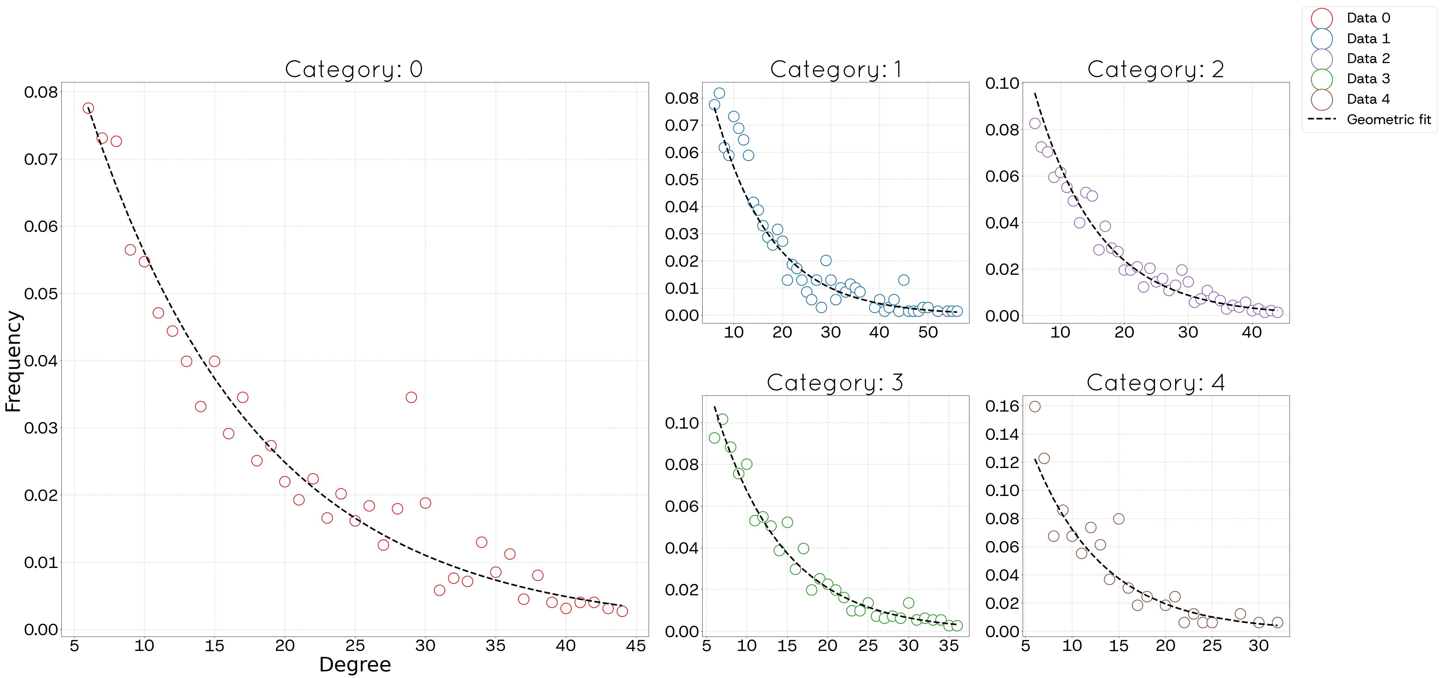
Each individual was categorized into 5 age groups, i.e., \(\mathcal{F} = \{0, 1,2,3,4\}\): [0,20) (youth, \(f=0\)), [20,30) (young adults, \(f=1\)), [30,50) (adults, \(f=2\)), [50,70) (senior adults, \(f=3\)), and 70 and older, representing the elderly (\(f=4\)). The left panel of Figure 2 shows the matrix, \(\mathbf{M}\), calculated from the average frequencies of connections from each age group in a row to an age group in a column. It is notable that the most frequent connections occur within the same age groups, as evidenced by the higher values along the main diagonal, with the exception of the last row. Additionally, there is a significant interaction with \(f=3\), likely because this group represents adults with children and those who may also care for elderly parents. Conversely, more distant age groups exhibit less interaction, as indicated by the lower values at the extremities of the matrix. The right panel of Figure 2 presents the distribution \(F\) of age groups. Figure 3 shows the degree distribution \(K(f)\) by age group of the respondents in the POLYMOD survey. Analysing the distribution of connections by age group reveals that the tail follows a geometric distribution, which can be written as \(P \propto (1 - \beta)^x \beta\) or \(P \propto e^{-\lambda x}(1 - e^\lambda)\). Considering the form \(P \propto e^{-\lambda x}(1 - e^\lambda)\), in Figure 3, the slope coefficient \(-\lambda\) and its corresponding \(R^2\) are determined for each age group using the least squares method.

Simulation results

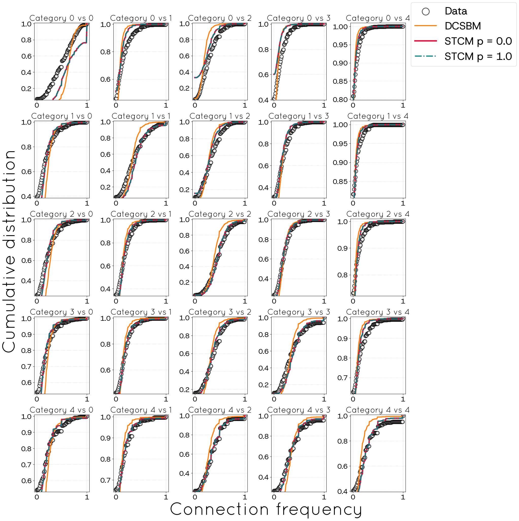
Since DCSBM and gHypEG require the knowledge of the complete graph for parameter estimation, we use the configuration model as a comparison benchmark. For both CM and STCM, nodes were distributed among groups according to the age distribution (see the right panel of Figure 2) and their degrees were selected at random according to age-dependent distributions (cf. Figure 3). STCM also makes use of the \(\mathbf{M}\) matrix (see left panel of Figure 2). We did our own implementation using the open source C library igraph. We start the study of the proposed algorithm by analysing the resulting frequency of connections between each pair of categories in the POLYMOD dataset. Figure 4 presents the cumulative frequency distributions taken from the empirical data, and the results the distribution of matrix of frequency of networks created using STCM (\(N= 300,000\) nodes) and CM (\(N= 100,000\) nodes) with a mean of 100 networks. As the results of the Stratified Configuration Model depend on the value of the clustering-enhancement probability \(p\), the results for the two extremes, \(p = 0\) and \(p = 1\), are presented, where it can be observed that the parameter \(p\) has no influence in the frequency of connection between categories. Observations indicate that the STCM yields a closer approximation to the original data than the CM, with the exception of interactions involving the first age category, where both algorithms present a similar performance.

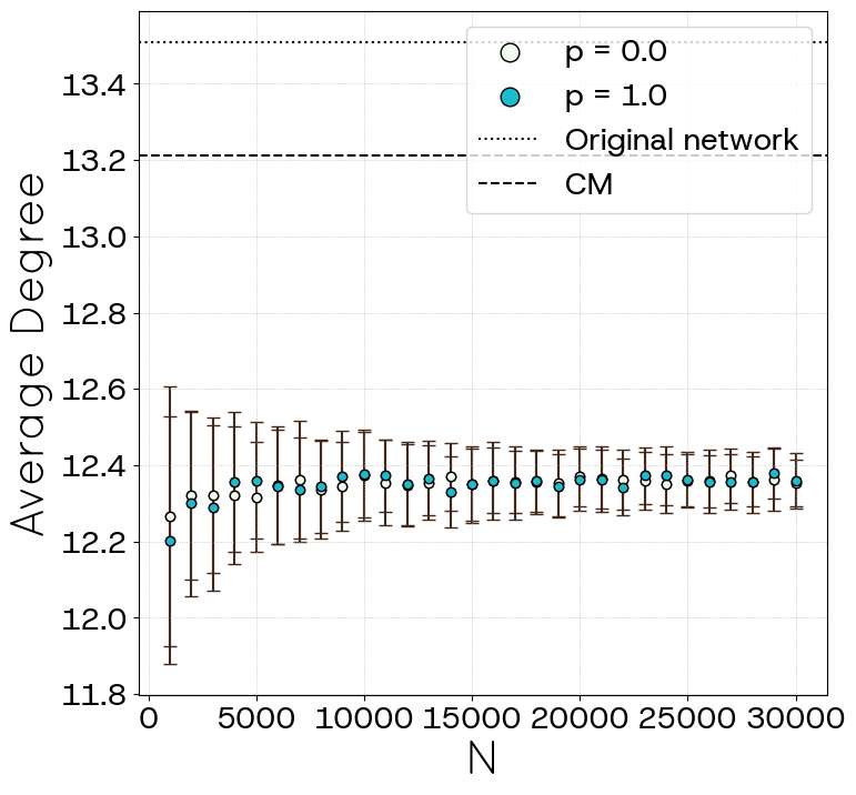
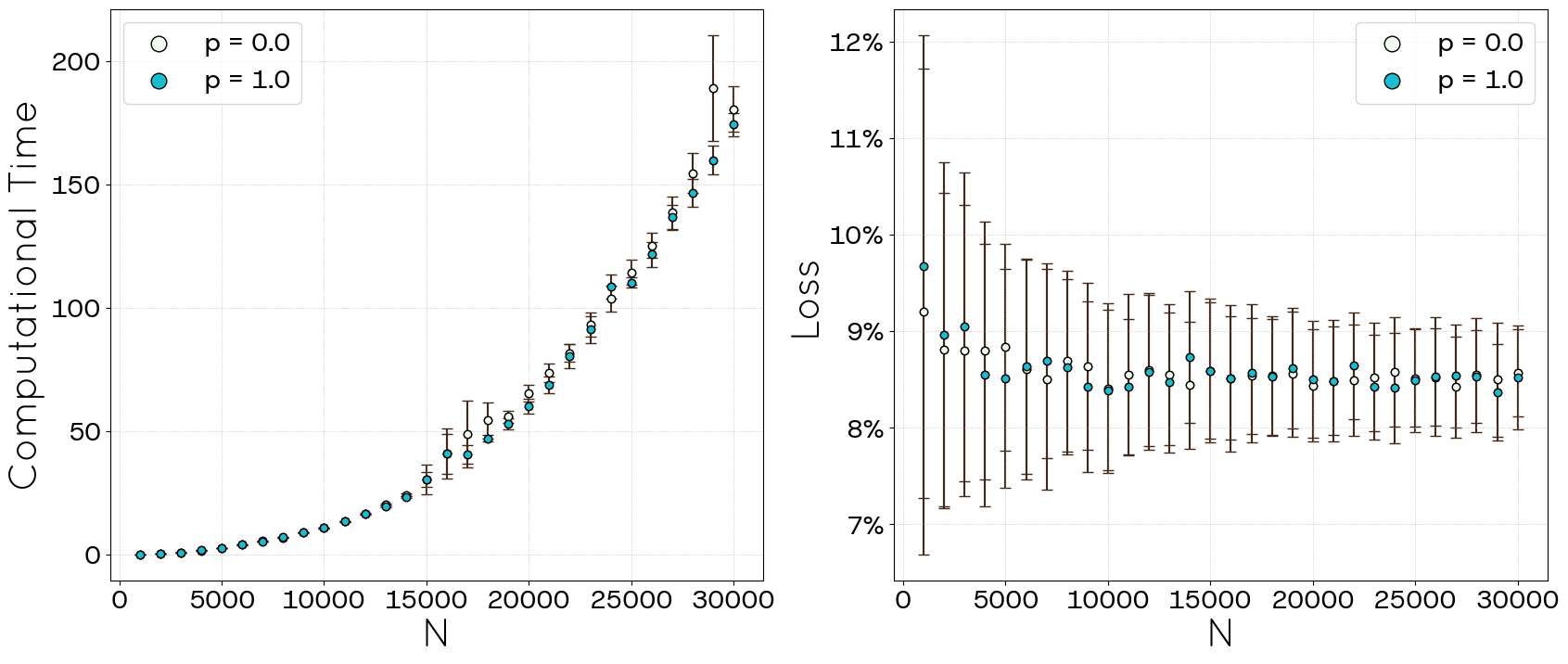
The mean degree obtained through STCM, depicted in Figure 5, deviates from the values documented in the collected data. This discrepancy, along with the performance observed in Figure 4, can be elucidated by examining Figure 6. The right panel of Figure 6 illustrates the percentage of discarded links (defined as the ratio of unallocated links to the total target number of links).

For smaller networks, this loss fraction approaches 9% but exhibits considerable fluctuation, reaching up to 12%. Conversely, for larger networks, the loss stabilizes near 8.5%. This link attrition is disproportionately concentrated within the first age category, which also possesses the highest connectivity. While this outcome represents an improvement over simpler models when input information is scarce, it remains suboptimal compared to the results achieved with the political blogs dataset where full network information is available. Furthermore, the left panel of Figure 6 displays the computation time as a function of network size (\(N\)). It reveals that the execution time exhibits weak dependence on the parameter \(p\) and scales polynomially with network size, approximately following \(t \propto N^{2.2}\). For the sake of reference, simulations were carried out on an INTEL H61 machine, with 16.0 GiB of RAM and an Intel Core i7-3770 CPU @ 3.40 GHz (8 processing cores). Programs were compiled in C using the igraph library for network simulations and executed in a single-threaded model. Graphs and averages were generated using Python, with data manipulation performed via NumPy and visualizations created using Matplotlib. The simulations were conducted under an Ubuntu 17.02 operating system.

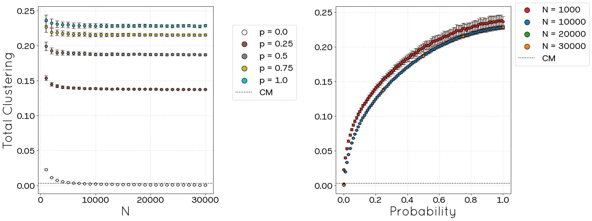
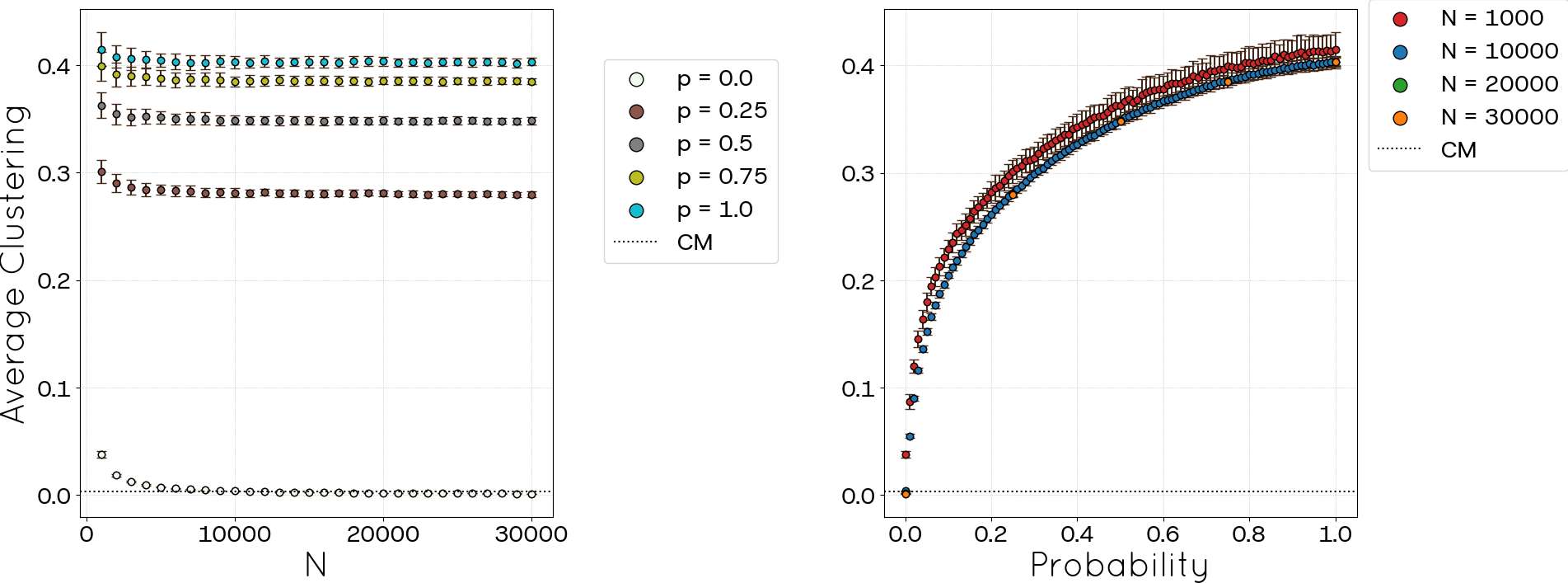
While the preceding metrics allowed for some comparison with empirical values, others, such as the global and average clustering coefficients, lack direct counterparts in the POLYMOD dataset; however, they can be compared against the CM baseline. Results for these metrics are presented in Figure 7 and Figure 8. The left panels in both figures illustrate the evolution of each clustering metric with network size (\(N\)) for different values of the parameter \(p\). Notably, for any given \(p\), the clustering coefficient initially decreases as \(N\) grows, eventually stabilizing. For \(p=0\), the total clustering coefficient stabilizes at approximately 0.03 (coinciding with the CM result), and the average clustering coefficient also reaches about 0.03. In contrast, at \(p=1.0\), these metrics attain significantly higher values, approximately 0.23 and 0.40, respectively, representing a roughly tenfold increase compared to the \(p=0\) case. The right panels demonstrate the variation of these metrics as a function of \(p\) for several network sizes. It is evident that for sufficiently large networks, the curves collapse onto a single trend, characterized by polynomial growth of the form \(Clustering \propto p^{\alpha}\), and the value of \(\alpha\) changes with \(N\).

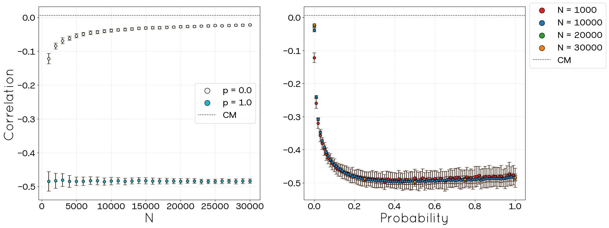
An analysis of the degree clustering correlation, presented in Figure 9, reveals a characteristic of the STCM in this context that is present in real networks (Bokányi et al. 2023). The algorithm effectively induces clustering primarily among low-degree nodes. High-degree nodes, which possess a larger number of potential neighbour combinations for triangle formation, exhibit comparatively lower clustering coefficients. This pattern appears to be independent of the network size \(N\).

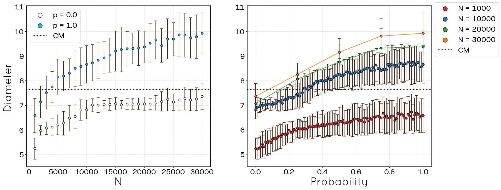
Two additional topological metrics investigated were the network diameter and the average shortest path length, shown in Figure 10 and Figure 11, respectively. Neither metric has a direct corresponding value in the original POLYMOD summary data. The diameter increases with both \(N\) and \(p\). For large \(N\), the diameter tends to stabilize around a value of 7 when \(p=0\), whereas for \(p=1.0\), it stabilizes near 10, albeit with greater variance. As the number of nodes in a network increases, it is expected that the number of peripheral nodes will grow, along with the network’s diameter. However, after reaching approximately 10.000 nodes, the diameter stabilizes. This stabilization occurs because the likelihood of adding connections to nodes that are not part of the diameter path is much higher than expanding the path itself or creating a new path of equivalent length. In sufficiently large networks, new links tend to connect nodes far from the diameter’s core, leading to denser structures without significantly altering the network’s diameter. The average shortest path length also demonstrates an increasing trend with both variables (\(N\) and \(p\)), in particular, the average shortest path grows with \(\log(N)\) for any value of \(p\), exhibiting a small-world trend.

Complete knowledge of the network: The political blogs case

Data

The second dataset is a study presented in the article of Adamic & Glance (2005) which analyses the interactions between political blogs during the 2004 U.S. presidential elections, a period when blogs exerted significant influence on political discourse and electoral engagement. The blogs were categorized into two main groups, i.e., \(\mathcal{F}=\{0,1\}\): liberal (\(f=0\)) and conservative (\(f=1\)), with the same amount of each (\(F(0)=F(1) = 0.5\)). The selection of the most influential blogs was based on metrics such as the number of citations in posts, using tools like BlogPulse. Additionally, the links between blogs, captured in a "snapshot" of a single day, included data extracted from blogrolls and citations found on main pages. Unlike the dataset used in previous studies, this database explicitly reflects the structural characteristics of a network, enabling detailed analyses of interactions and connectivity patterns among blogs.

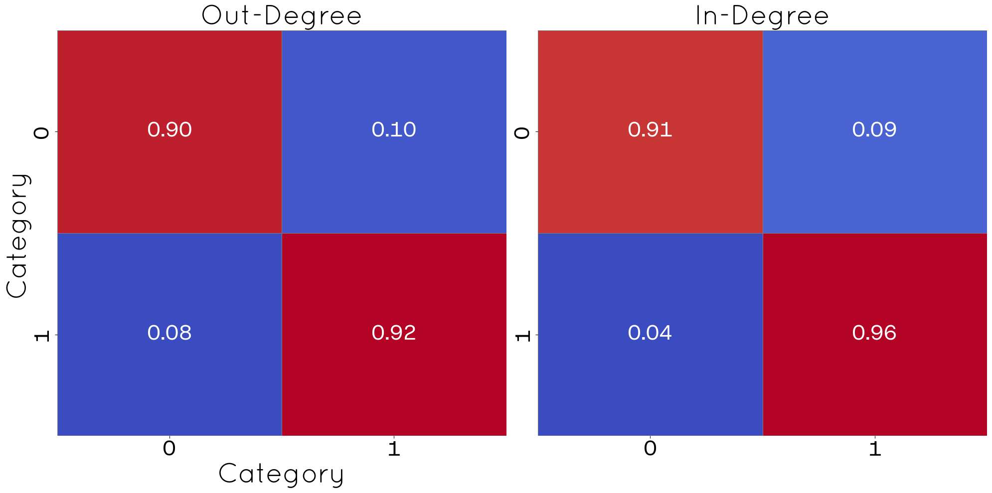
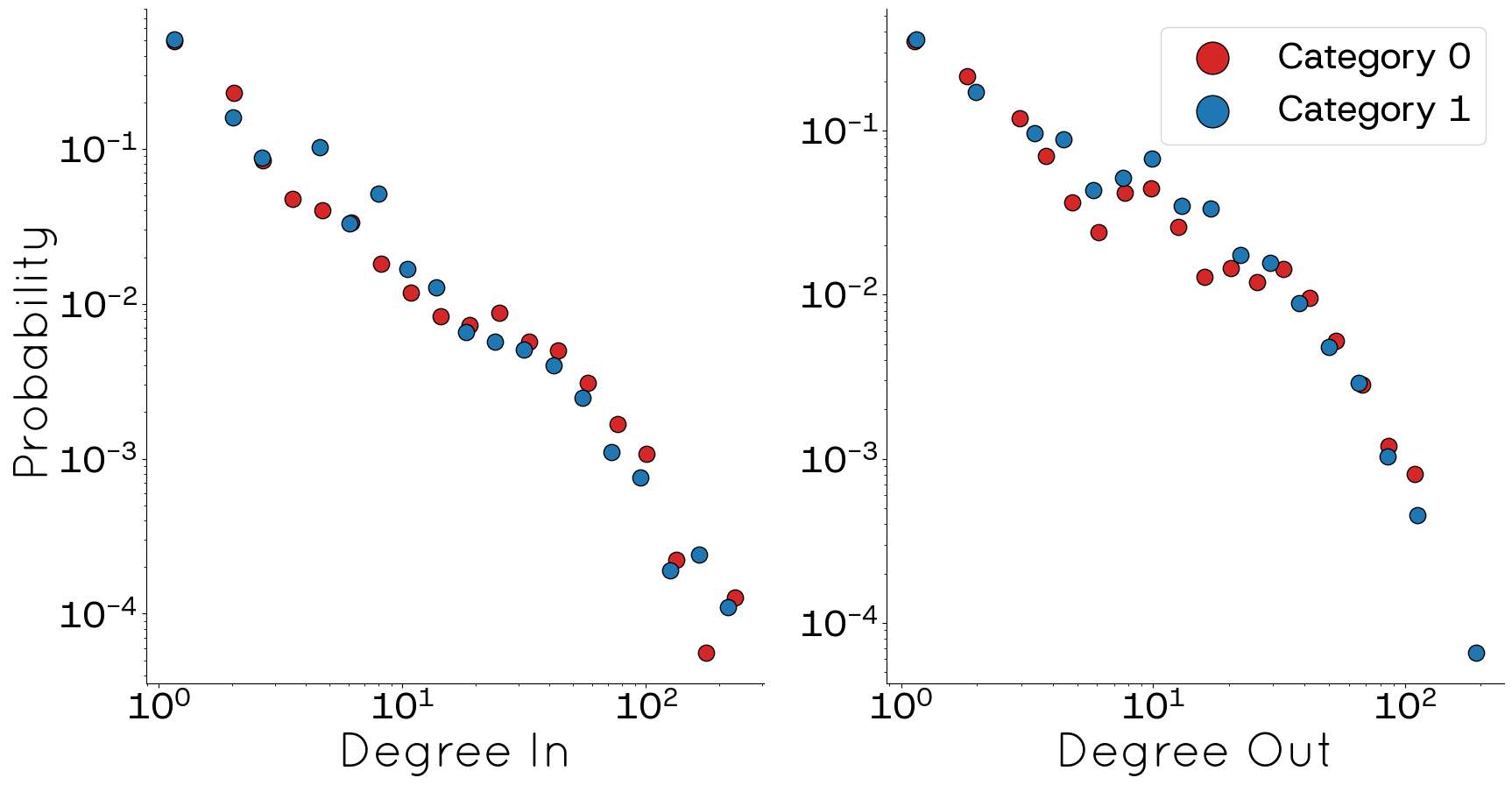
Since the original dataset is already structured as a network, it was possible to compute essential metrics for our analysis. For example, the network comprises 793 nodes and 15783 edges (the strongly connected component of the network), with a total clustering coefficient of 0.197, an average clustering coefficient of 0.21, and an average degree of 31. Figure 12 displays the matrices \(\mathbf{M}^{in}\) and \(\mathbf{M}^{out}\) of the blog network, highlighting that more than 80% of the connections occur between blogs sharing similar political views. It is noteworthy that, on average, blogs in both categories tend to be referenced more by their peers than they reference those within their own group. Finally, Figure 13 shows the degree distribution for both in-links (\(K^{in}\)) and out-links (\(K^{out}\)) in each category. Although the distribution exhibits a sharp decline, similar to that observed in POLYMOD, it does not exactly mirror the latter’s pattern.

Simulation results

Since we have complete knowledge of the graph, we can estimate the parameters of the Degree-Corrected Stochastic Block Model and the Block-Constrained Generalized Hypergeometric Model. In both cases, we changed the size of the generated network by making copies of the nodes in the dataset. For DCSBM, we used the graph-tool Python package; in the case of gHypEG, we used an open source library in R (Casiraghi & Nanumyan 2024). We must note that we do not present results with the CM as they do not give more information beyond that in the case of the POLYMOD dataset and for the sake of clarity in the following paragraphs.

In contrast to the POLYMOD case, the analysis of the political blogs dataset benefits from complete knowledge of the network structure. This allows for the evaluation of additional metrics and provides a different perspective on the STCM’s performance. Here, network size is often represented by \(N^*\), denoting the number of replications or copies of the original node set (see Algorithm 3).

For instance, Figure 14 illustrates the STCM’s (for \(p=0\) and \(p=1.0\)) capability (using \(N^{*} = 20\) copies) in reproducing the inter-category connection frequencies. The Stratified Configuration Model achieves a notably better replication of these mesoscale structures than observed in the POLYMOD case. Interestingly, the generalized hypergeometric model performs much worse than DCSBM and STCM.

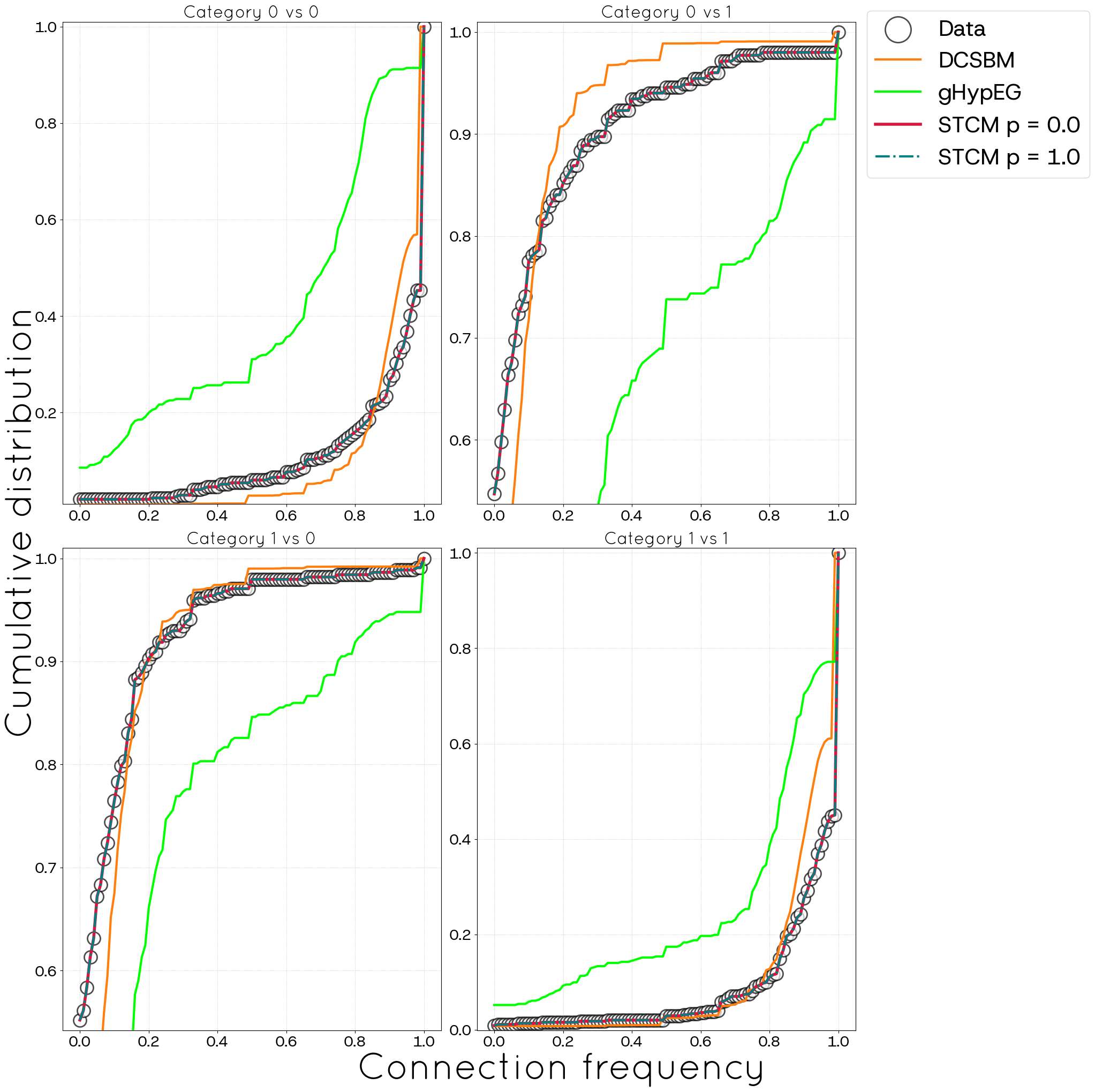
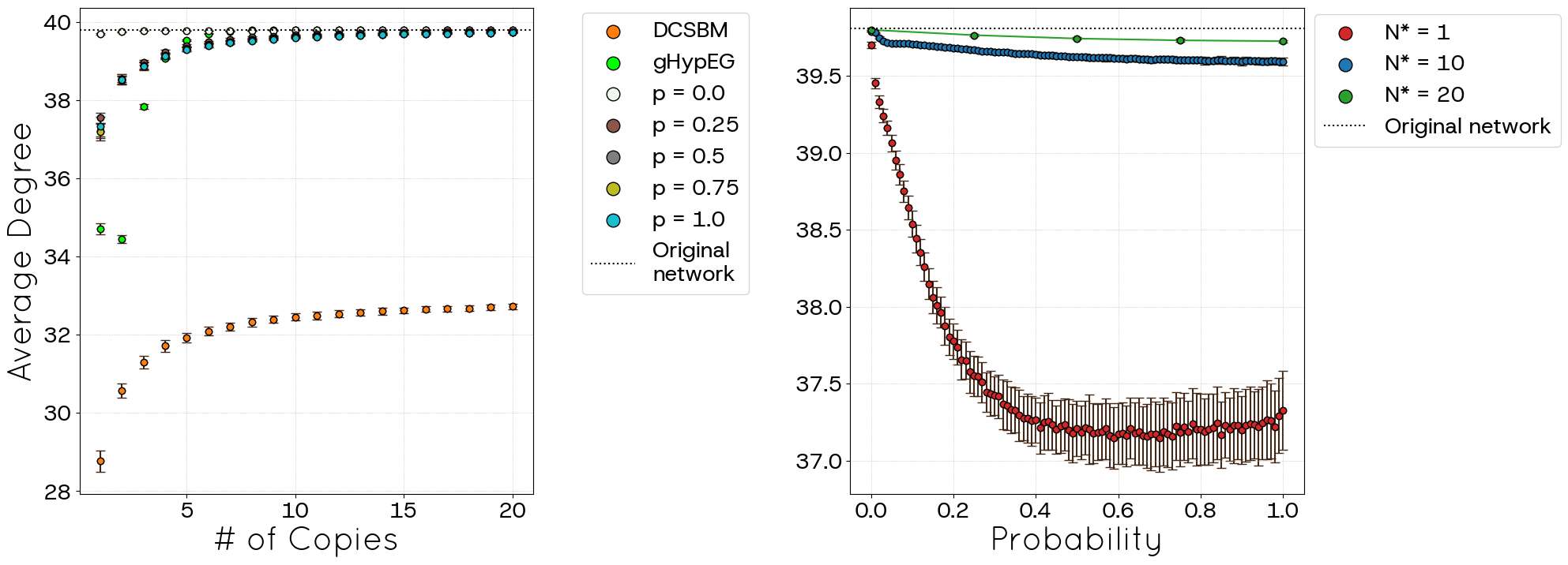
Figure 15 shows the mean degree as a function of \(N^{*}\) and \(p\). For \(p=0\), STCM accurately reproduces the empirical mean degree regardless of \(N^*\), outperforming DCSBM and gHypEG. Surprisingly, results for DCSBM are much worse than those for the gHypEG model and STCM, which exhibit a similar performance. Indeed, the degree-correlated stochastic block model generates self-loops and multiple links. As these types of connections do not make sense in the context of the political blogs dataset, they were removed, leading to a lower average degree as consequence. Since STCM does not produce self-loops and multiple links, the average degree is closer to that of the original network. When \(p=1.0\), however, a larger network size (i.e., greater \(N^*\)) is necessary for STCM to closely approximate the empirical value; smaller \(N^*\) values lead to larger deviations and increased variance. Please observe that, due to computational constraints for \(N^* > 10\), we restricted the analysis to the values of \(p\) in \(\{0.00, 0.25, 0.50, 0.75, 1.00\}\).

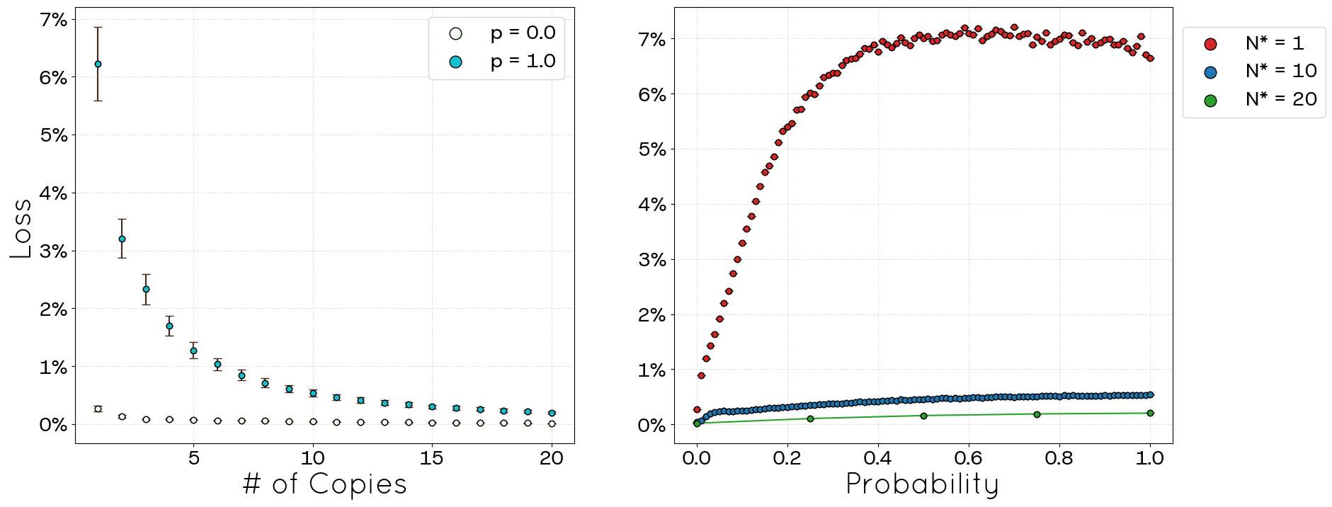
These observations are consistent with the link loss behaviour shown in Figure 16. For \(p=0\), the link loss is minimal, approximately 0.3%. As \(p\) increases, aiming for higher clustering, the loss fraction grows, reaching about 7% for \(p=1.0\) (still considerably lower than in the POLYMOD case). Importantly, this loss diminishes as the network size (\(N^*\)) increases. This suggests a trade-off inherent in the STCM: enhancing clustering (increasing \(p\)) while simultaneously attempting to precisely replicate the degree sequence and inter-category connection frequencies inevitably leads to a higher number of unallocated links.

Figures 17 and 18 display the results for global and average clustering, respectively, now with the benefit of empirical benchmark values (indicated by dotted lines). For average clustering, setting \(p=0\) and \(N^{*}=1\) yields a value (approx. \(0.38\)) exceeding that of the original network. However, as \(N^*\) increases, the average clustering rapidly declines, stabilizing around \(0.03\) for large \(N^*\). A similar trend occurs for \(p=1.0\), starting higher (approx. \(0.53\)) and decreasing towards \(0.50\) as \(N^*\) grows and the curve has a polynomial fit \(Clustering \propto p^{\alpha}\) where \(\alpha\) depends on \(N^*\). In all cases, higher values of \(p\) lead to higher clustering. As for DCSBM, observe that it exhibits very low clustering, never reaching the value of the original network. On the contrary, gHypEG always presents clustering values larger than that of the dataset.

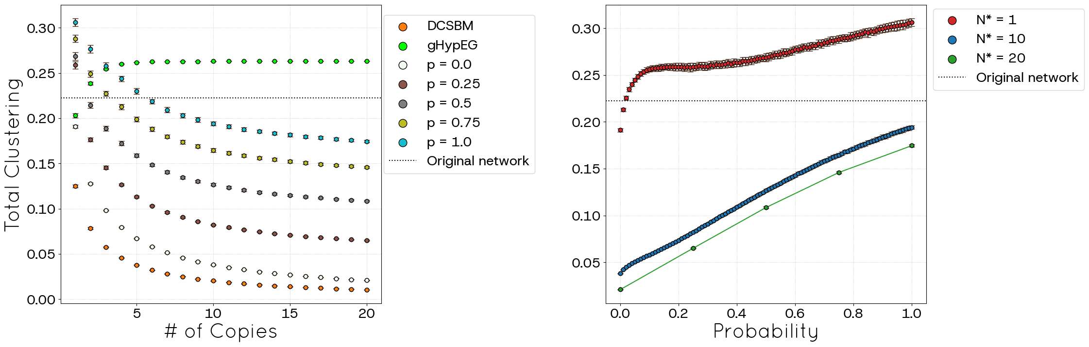
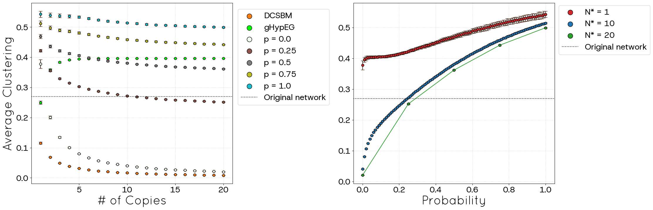
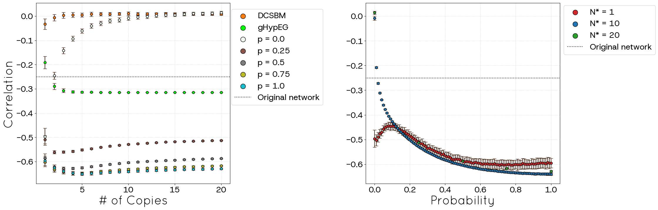
Figure 19 presents the degree-clustering correlation in the analysed network. With \(p=0\), networks generated with small \(N^*\) exhibit a negative correlation, indicating reduced clustering among high-degree nodes. However, as \(N^*\) increases, this correlation weakens, approaching an uncorrelated state similar to that of DCSBM. Although this result of the political blogs resembles that described in the POLYMOD case, in the latter case the correlation does not reach zero as it does in the former. Conversely, when \(p=1.0\), a strong negative correlation persists and is even more pronounced than that observed in the POLYMOD analysis, regardless of \(N^*\). Most interestingly, gHypEG also exhibits a negative correlation, but of a similar magnitude to that of the original dataset.

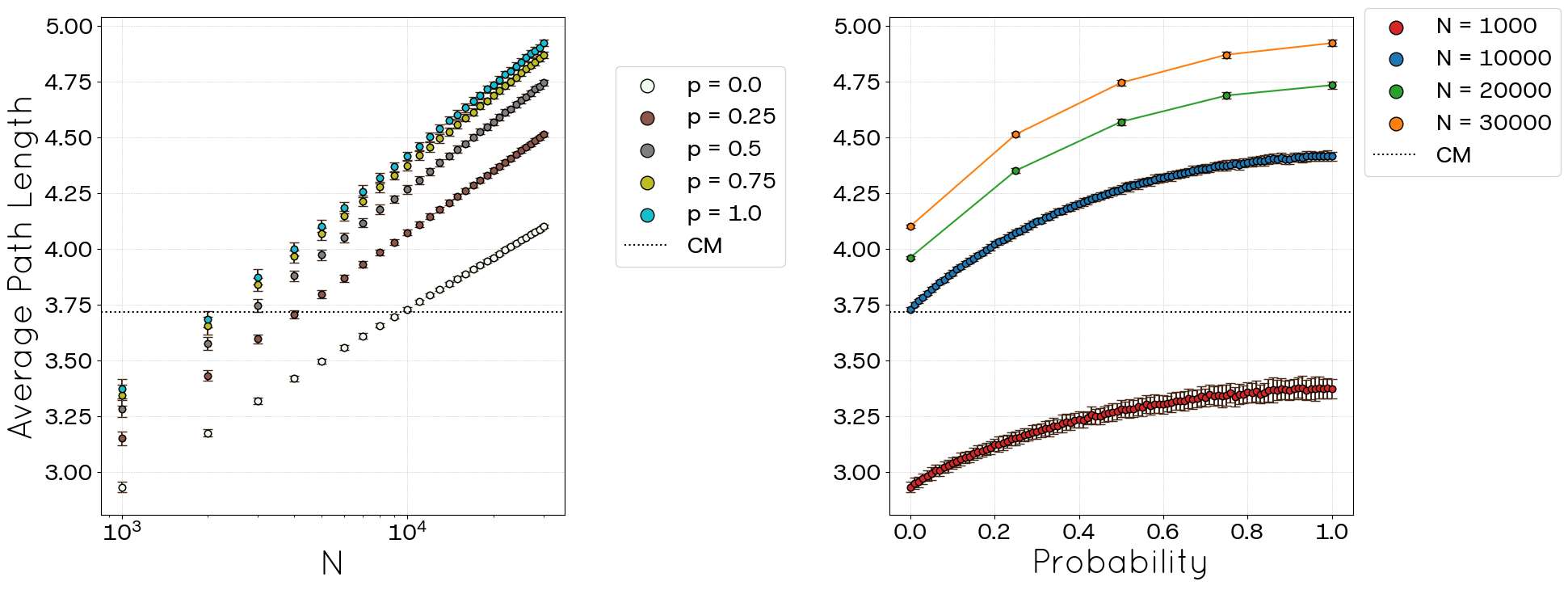
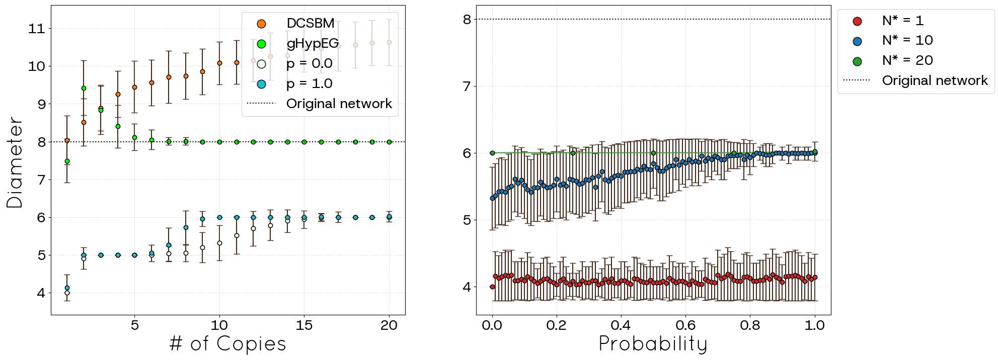
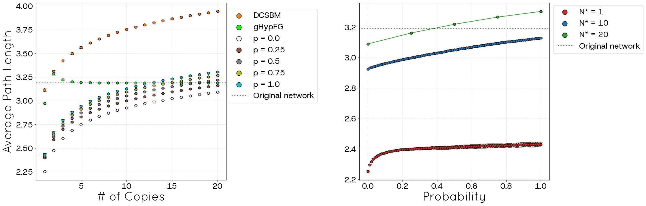
Figures 20 and 21 present the diameter and the average shortest path length, respectively. The diameter displays a distinct evolution compared to POLYMOD. For \(p=0\), starting from an average of 4 for \(N^{*}=1\), it stabilizes around 5 for \(N^*\) up to 8, and then increases slightly to stabilize around 6 for \(N^*\) up to 15. A similar, potentially faster, non-monotonic pattern is observed for \(p=1.0\). The right panel confirms the dependence on \(p\). In both scenarios, the generated diameters do not reach the empirical value of the original network because the model focuses on maintaining fidelity with the degree distribution and more complex metrics are not necessarily mimicked correctly. The average shortest path length follows the previously observed trend, increasing with both \(p\) and the number of copies \(N^*\) and exhibiting the same behaviour of POLYMOD. Let us note that the generalized hypergeometric model correctly reproduces the network diameter and the average shortest path length for most of the network sizes, outperforming both DCSBM and STCM.

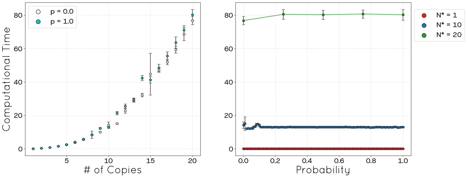
Finally, Figure 22 confirms that the computational time scaling for the political blogs dataset is analogous to the POLYMOD case. The time complexity shows only a weak dependence on the parameter \(p\) and exhibits polynomial growth with the effective network size (\(N^*\)), consistent with the \(t \propto N^{2.2}\) scaling observed earlier.

Conclusion

Existing network generation models, particularly the standard Configuration Model, often fall short in capturing crucial topological features observed in real-world networks, such as high clustering coefficients and the tendency for nodes with similar attributes to connect preferentially (homophily). The failure to incorporate node characteristics into the link formation process and the inherently low triangle formation in the CM limit its applicability for generating realistic synthetic graphs.

In this work, we introduced the Stratified Configuration Model, explicitly designed to overcome these limitations. The STCM directly integrates nodal attributes through network stratification into categories and implements a tunable mechanism, controlled by the parameter \(p\), to actively promote triad formation.

Our evaluations, utilizing the POLYMOD (partial information) and political blogs (full information) datasets, demonstrate the effectiveness of the STCM. The model significantly improves the ability to reproduce the observed frequency of connections between different node categories (Figures 4, 14), directly addressing the need to consider node characteristics. Furthermore, the STCM successfully generates networks with substantially higher global and average clustering coefficients than the CM, which are tunable via the parameter \(p\) (Figures 7, 8, 17, 18). In scenarios with complete information (e.g., the political blogs case), the STCM was able to achieve clustering levels comparable to the empirical network, overcoming the fundamental low-clustering limitation of the CM.

Despite these advancements, the STCM exhibits certain trade-offs. We observed a percentage of link loss (unallocated links), particularly pronounced when targeting high clustering values (high \(p\)) or operating with incomplete network information (POLYMOD), although this behaviour tends to decrease with increasing network size (Figures 6, 16). This loss can consequently affect the precise replication of the mean degree in some regimes (Figures 5, 15). Additionally, the current triad formation mechanism tends to favour low-degree nodes, resulting in a negative degree-clustering correlation that may not align with all empirical network structures (Figures 9, 19). Other global metrics, such as diameter and average path length, are also influenced by the introduction of clustering via parameter \(p\) (Figures 10, 11, 20, 21).

We performed a thorough comparison with the Configuration Model, the Degree-Corrected Stochastic Block Model and the Block-Constrained Generalized Hypergeometric Model. We have shown that STCM outperforms CM and DCSBM in all cases. However, the gHypEG model exhibits better results in terms of network diameter and average path degree. One problem of gHypEG, though, is that it requires the knowledge of the complete network in order to estimate its parameters. The Stratified Configuration Model, on the contrary, can deal with incomplete knowledge as it was shown in the POLYMOD example.

We must note that, as an anonymous reviewer observed, STCM can be used as a null model for the analysis of completely known networks. Indeed, the Stratified Configuration Model only assumes the knowledge of group-dependent input and output degree distributions and intergroup connection frequencies (at least for a rewiring probability \(p=0\)). Any structure found beyond that predicted by STCM must be assumed as not determined by that information.

All in all, the STCM represents a valuable step towards generating more realistic synthetic networks by integrating mesoscale group structures (stratification) and microscale clustering properties in a controlled manner. Its demonstrated polynomial time complexity (\(t \propto N^{2.2}\) or \(N^{*2.2}\)) (Figures 6, 22) ensures scalability for moderately sized networks.

Future research should focus on refining the link allocation process to minimize loss, especially under strong clustering constraints, and exploring alternative mechanisms to achieve desired clustering patterns across the degree spectrum, potentially addressing the observed bias in degree-clustering correlation. Continued improvement of models like the STCM is essential for providing robust tools for studying complex systems where both node attributes and local network structure play critical roles.

References

ABE, S., & Suzuki, N. (2004). Scale-free network of earthquakes. Europhysics Letters (EPL), 65(4), 581–586.

ADAMIC, L. A., & Glance, N. (2005). The political blogosphere and the 2004 U.S. election: Divided they blog. Proceedings of the 3rd International Workshop on Link Discovery.

ALBERT, R. (2005). Scale-free networks in cell biology. Journal of Cell Science, 118(21), 4947–4957.

BARABÁSI, A.-L., & Albert, R. (1999). Emergence of scaling in random networks. Science, 286(5439), 509–512.

BASSETT, D. S., & Bullmore, E. (2006). Small-world brain networks. The Neuroscientist, 12(6), 512–523.

BESAG, J. (1986). On the statistical analysis of dirty pictures. Journal of the Royal Statistical Society Series B: Statistical Methodology, 48(3), 259–279.

BHATTACHARYA, K., Mukherjee, G., Saramäki, J., Kaski, K., & Manna, S. S. (2008). The international trade network: Weighted network analysis and modelling. Journal of Statistical Mechanics: Theory and Experiment, 2008(02), P02002.

BIANCONI, G. (2007). The entropy of randomized network ensembles. Europhysics Letters (EPL), 81(2), 28005.

BOKÁNYI, E., Heemskerk, E. M., & Takes, F. W. (2023). The anatomy of a population-scale social network. Scientific Reports, 13(1).

CASIRAGHI, G. (2019). The block-constrained configuration model. Applied Network Science, 4(1), 123.

CASIRAGHI, G., & Nanumyan, V. (2021). Configuration models as an urn problem. Scientific Reports, 11(1), 13416.

CASIRAGHI, G., & Nanumyan, V. (2024). ghypernet: Fit and simulate generalised hypergeometric ensembles of graphs. Available at: https://ghyper.net

CASIRAGHI, G., Nanumyan, V., Scholtes, I., & Schweitzer, F. (2016). Generalized hypergeometric ensembles: Statistical hypothesis testing in complex networks. arXiv preprint. Available at: https://arxiv.org/abs/1607.02441

CHATTERJEE, S., & Diaconis, P. (2013). Estimating and understanding exponential random graph models. The Annals of Statistics, 41(5), 2428–2461.

CHRISTAKIS, N. A., & Fowler, J. H. (2007). The spread of obesity in a large social network over 32 years. New England Journal of Medicine, 357(4), 370–379.

CHUNG, F., & Lu, L. (2002a). Connected components in random graphs with given expected degree sequences. Annals of Combinatorics, 6(2), 125–145.

CHUNG, F., & Lu, L. (2002b). The average distances in random graphs with given expected degrees. Proceedings of the National Academy of Sciences, 99(25), 15879–15882.

DROBYSHEVSKIY, M., & Turdakov, D. (2019). Random graph modeling: A survey of the concepts. ACM Computing Surveys, 52(6), 1–36.

ERDŐS, P., & Rényi, A. (1959). On random graphs. I. Publicationes Mathematicae, 6(3–4), 290–297.

FRANK, O., & Strauss, D. (1986). Markov graphs. Journal of the American Statistical Association, 81(395), 832–842.

GEYER, C. J., & Thompson, E. A. (1992). Constrained Monte Carlo maximum likelihood for dependent data. Journal of the Royal Statistical Society: Series B (Methodological), 54(3), 657–683.

GONÇALVES, M., Fierens, P. I., & Rêgo, L. C. (2026). A new take on optimal vaccine prioritization: When age-based strategy is efficient? International Journal of Data Science and Analytics, 22, 95.

GOODREAU, S. M. (2007). Advances in exponential random graph (p*) models applied to a large social network. Social Networks, 29(2), 231–248.

HANDCOCK, M. S. (2003). Assessing degeneracy in statistical models of social networks. Center for Statistics and the Social Sciences, University of Washington, Working paper no. 39.

HE, R., & Zheng, T. (2013). Estimation of exponential random graph models for large social networks via graph limits. Proceedings of the 2013 IEEE/ACM International Conference on Advances in Social Networks Analysisand Mining

KARRER, B., & Newman, M. E. J. (2011). Stochastic blockmodels and community structure in networks. Physical Review E, 83(1).

KIM, K., & Altmann, J. (2017). Effect of homophily on network formation. Communications in Nonlinear Science and Numerical Simulation, 44, 482–494.

KLISE, K., Beyeler, W., Acquesta, E., Thelen, H., Makvandi, M., & Finley, P. (2022). Prioritizing vaccination based on analysis of community networks. Applied Network Science, 7(1).

LATORA, V., & Marchiori, M. (2002). Is the Boston subway a small-world network? Physica A: Statistical Mechanics and Its Applications, 314(1), 109–113.

LEE, C., & Wilkinson, D. J. (2019). A review of stochastic block models and extensions for graph clustering. Applied Network Science, 4(1), 122.

LESKOVEC, J., Chakrabarti, D., Kleinberg, J., Faloutsos, C., & Ghahramani, Z. (2010). Kronecker graphs: An approach to modeling networks. Journal of Machine Learning Research, 11(33), 985–1042.

MANZO, G., & van de Rijt, A. (2020). Halting SARS-CoV-2 by targeting high-contact individuals. Journal of Artificial Societies and Social Simulation, 23(4), 10.

MCPHERSON, M., Smith-Lovin, L., & Cook, J. M. (2001). Birds of a feather: Homophily in social networks. Annual Review of Dociology, 27(1), 415–444.

MOSSONG, J., Hens, N., Jit, M., Beutels, P., Auranen, K., Mikolajczyk, R., Massari, M., Salmaso, S., Scalia Tomba, G., Wallinga, J., Heijne, J., Sadkowska-Todys, M., Rosinska, M., & Edmunds, W. J. (2017). POLYMOD social contact data. Available at: https://doi.org/10.5281/zenodo.3746312

MOSSONG, J., Hens, N., Jit, M., Beutels, P., Auranen, K., Mikolajczyk, R., Massari, M., Salmaso, S., Tomba, G. S., Wallinga, J., Heijne, J., Sadkowska-Todys, M., Rosinska, M., & Edmunds, W. J. (2008). Social contacts and mixing patterns relevant to the spread of infectious diseases. PLoS Medicine, 5(3), e74.

NEWMAN, M. (2018). Networks. Oxford: Oxford University Press.

OLIVEIRA, R., Brito, S., da Silva, L. R., & Tsallis, C. (2022). Statistical mechanical approach of complex networks with weighted links. Journal of Statistical Mechanics: Theory and Experiment, 2022(6), 063402.

PARK, J., & Newman, M. E. J. (2004). Statistical mechanics of networks. Physical Review E, 70(6).

PEIXOTO, T. P. (2014). Hierarchical block structures and high-resolution model selection in large networks. Physical Review X, 4(1).

PEIXOTO, T. P. (2019). Bayesian stochastic blockmodeling. In Advances in Network Clustering and Blockmodeling (pp. 289–332). Hoboken, NJ: John Wiley & Sons.

ROBINS, G., Pattison, P., Kalish, Y., & Lusher, D. (2007). An introduction to exponential random graph (p*) models for social networks. Social Networks, 29(2), 173–191.

SNIJDERS, T. A. (2002). Markov chain Monte Carlo estimation of exponential random graph models. Journal of Social Structure, 3(2), 1–40.

STRAUSS, D., & Ikeda, M. (1990). Pseudolikelihood estimation for social networks. Journal of the American Statistical Association, 85(409), 204–212.

VAN der Hoorn, P., Lippner, G., & Krioukov, D. (2017). Sparse maximum-entropy random graphs with a given power-law degree distribution. Journal of Statistical Physics, 173(3–4), 806–844.

WATTS, D. J., & Strogatz, S. H. (1998). Collective dynamics of small-world networks. Nature, 393(6684), 440–442.

ZHOU, Y., & ZHOU, J. (2018). Algorithm for multiplex network generation with shared links. Physica A: Statistical Mechanics and Its Applications, 509, 945–954.