S-Frame Vs. I-Frame Interventions: The Transformation-Robustness Trade-off in Behavioural Policy

aNational University of Singapore, Singapore; b University of Trento, Italy
Journal of Artificial
Societies and Social Simulation 29 (3) 1
<https://www.jasss.org/29/3/1.html>
DOI: 10.18564/jasss.6041
Received: 18-Oct-2025 Accepted: 31-Mar-2026 Published: 30-Jun-2026
Abstract
This paper evaluates the risk–benefit profiles of individual-level (i-frame) and system-level (s-frame) behavioural interventions using an agent-based model (ABM). The i-frame/s-frame distinction refers to whether policy targets individual behaviour change (e.g., nudges, information campaigns) or systemic structures (e.g., regulations, network-based seeding). We formalise and test three policy-relevant risks: (A) structural misspecification risk (errors in the network used for targeting), (B) heterogeneity risk (adverse or weakly responsive subpopulations), and (C) shock risk (temporary dampening vs. backsliding of behaviour). For each dimension, we track four outcomes: adoption levels achieved, diffusion speed, cost-efficiency, and downside risk (measured by the share of runs ending below 10% adoption). Two findings stand out. First, when structural assumptions are approximately correct, targeted s-frame seeding ignites cascades and is markedly more transformative and cost-efficient than i-frame benchmarks. Second, the same reliance on social spillovers creates fragility:mis-targeting and backsliding shocks substantially reduce performance, whereas i-frame designs deliver smaller but steadier gains and degrade more gently. The results imply a portfolio approach: measurement-first targeting and staged rollout to earn the right to scale s-frame power, coupled with i-frame backstops and simple shock absorbers to keep systems in a safe-to-fail corridor. The framework provides actionable guidance for choosing and sequencing policy levers under uncertainty while making risk explicit.I-frame (individual frame): Policy interventions targeting individual behaviour change through mechanisms such as nudges, defaults, information provision, or incentives that operate at the person level.
S-frame (system frame): Policy interventions targeting systemic structures through mechanisms such as regulation, taxation, institutional reform, or network-based seeding that reshape the environment in which choices occur.
Misspecification: A mismatch between a policy's intended logic and the conditions under which it is designed or implemented, so that intended effects do not materialise or unintended effects dominate.
Spillovers: Indirect effects whereby an intervention's impact on targeted individuals spreads to non-targeted individuals through social networks or environmental changes.
Introduction
The debate opened by Chater & Loewenstein (2022) in Behavioral and Brain Sciences (BBS) has pushed behavioural public policy to confront a fundamental question: should policy focus primarily on changing individual behaviour, or on changing the wider systems within which behaviour occurs? In this literature, these alternatives are referred to as i-frame and s-frame interventions. The former refers to person-level tools such as nudges, defaults, or information campaigns, while the latter aims to alter the broader environment through regulation, taxation, institutional redesign, or targeted changes to social structure. Related distinctions between downstream and upstream interventions, and between higher- and lower-agency policy instruments, have also been developed in adjacent public health and policy literatures (Adams et al. 2016; Lorenc et al. 2013). These differences also tend to map onto disciplinary specialisms, with behavioural scientists and experimental economists more often focusing on person-level instruments, and sociologists, economists, legal scholars, and political scientists more often emphasising systemic levers (Chater & Loewenstein 2022; Connolly et al. 2025). This debate echoes parallel questions about how micro-level decisions generate macro-level patterns, which have long been central to sociology and to the literature on policy diffusion (Berry & Berry 1990; Coleman 1990; Shipan & Volden 2008; Walker 1969).
While providing a full synthesis of these debates for an interdisciplinary audience would be an important contribution in itself, our aim here is narrower and more specific to behavioural public policy. Although alternative policy frames have fuelled a lively debate, evidence to compare them systematically has remained largely qualitative. A formal comparative account of when system-level interventions outperform individual-level ones, and when their broader reach makes them more fragile, is still missing.
The present paper does not attempt a full synthesis with those broader literatures. Instead, it uses the i-/s-frame vocabulary to speak directly to the behavioural public policy audience that has engaged with the BBS exchange, while translating the debate into a transparent mechanism-based model. Our starting point is policy misspecification. By this, we mean failures that arise when the assumptions built into a policy do not match the social structure, behavioural response, implementation conditions, or wider environment in which the policy is deployed. This framing matters because the central practical question is not simply whether system-level interventions can produce larger effects. Rather, it is whether their larger reach also amplifies the consequences of error. Person-level interventions often yield modest gains, but they are typically easier to reverse and their failures remain relatively localised. System-level interventions can be far more transformative, yet they can also propagate mistakes through networks, institutions, and implementation chains (Arthur 1989; Howlett 2012; McConnell 2014; Pierson 2000).
Agent-based modelling (ABM) is useful for studying this problem because the relevant trade-off depends on interaction effects that cannot be read off average treatment effects alone. Spillovers, local reinforcement, threshold effects, heterogeneous response, and external shocks can all change whether an intervention remains small and steady or becomes self-reinforcing and fragile. A simulation framework therefore allows us to compare intervention families under controlled changes in the conditions that matter most for misspecification.
The paper examines three experimental dimensions that correspond to recurring sources of misspecification in the policy literature. The first is network information error: how system-level targeting performs when policy-makers have an inaccurate view of the social structure they are trying to influence. The second is heterogeneous response: how results change when part of the population responds weakly or adversely to the intervention. The third is shock resilience: whether temporary external disturbances merely slow progress or instead induce behavioural backsliding. Across these dimensions, we compare final adoption, diffusion speed, cost-efficiency, and downside risk.
Scoping Review: Sources of Policy Misspecification
Review methodology
This scoping review synthesises documented cases of public policy misspecification that led to adverse effects, with a particular focus on the underlying reasons for these failures. Following established scoping review guidelines (Arksey & O’Malley 2005), we searched the policy studies, public administration, and behavioural policy literatures using terms including “policy failure,” “implementation failure,” “unintended consequences,” and “policy misspecification.” We focused on sources that: (a) documented specific cases or categories of policy failure, (b) analysed the mechanisms underlying failure, and (c) offered conceptual frameworks for understanding misspecification. The review prioritised foundational works in policy studies (Matland 1995; Pressman & Wildavsky 1973; Sabatier & Mazmanian 1980) and influential syntheses (Howlett 2012; McConnell 2010, 2014). The purpose of the review is not to produce an exhaustive census of all policy failures. Rather, it identifies the types of misspecification most relevant to comparing i-frame and s-frame interventions and uses them to motivate the simulation design.
Seven categories of misspecification
The review revealed seven recurring ways in which policies become misspecified. The categories are described first in plain language and only then translated into model components.
Conceptual and design problems. These arise when policy goals, instruments, and target populations are poorly aligned. The classic problem is not merely that a policy is weak or strong, but that its logic does not fit the mechanism through which change is supposed to occur. Overinclusive targeting, poor proxy measures, or a mismatch between the policy tool and the behavioural process all belong in this category (Howlett 2012).
Information and knowledge deficits. Policies are often designed with incomplete or misleading information about the populations, organisations, or social structures they seek to change. In behavioural policy, this includes weak knowledge of who influences whom, how fast effects decay, or which groups are likely to respond. Failures of this kind are especially consequential when policy depends on accurate targeting or on assumptions about diffusion pathways.
Political and institutional distortions. Even when policymakers understand the problem, political incentives and institutional pressures can redirect implementation toward administratively convenient or politically valuable targets rather than substantively appropriate ones. Interest-group influence, electoral time pressure, or centralised decision-making without local adaptation are common examples (Flyvbjerg 2009).
Capacity and resource constraints. Policies can also fail because implementing organisations lack the time, staff, funding, or coordination capacity needed to deliver them as designed. A strategy that is sound in principle may still underperform if it cannot be deployed at the right scale, in the right places, or for long enough.
Process and stakeholder failures. Policies frequently depend on cooperation, legitimacy, and local learning. Weak participation, poor communication, or a failure to anticipate how subgroups will react can lower responsiveness and undermine adaptation during implementation (Moynihan et al. 2015).
Complexity and uncertainty challenges. Some policy settings are characterised by strong interdependence, delayed effects, or external shocks that are difficult to anticipate in advance. In these settings, the problem is not only imperfect information but also genuine instability in the environment, which can weaken or reverse the expected trajectory of change (Head 2008; Rittel & Webber 1973).
Governance and implementation gaps. Finally, policies may fail because they are not monitored, adjusted, or coordinated once deployment begins. The greater the reach of the intervention, the more costly it can be when errors are locked in and allowed to propagate through administrative routines or path-dependent institutional arrangements (Arthur 1989; Matland 1995; McConnell 2010; Pierson 2000; Pressman & Wildavsky 1973; Sabatier & Mazmanian 1980).
Linking misspecification categories to the simulation design
The ABM does not attempt to represent all seven categories in their full real-world complexity. Instead, it uses them to define a smaller set of experimentally tractable questions. Network information errors represent the informational side of misspecification; heterogeneous response captures design, process, and stakeholder problems; and external shocks capture complexity, uncertainty, and implementation stress. The crosswalk in Table 1 shows how each category is represented and which outcome dimensions it is expected to affect most strongly.
| Misspecification Category | Illustrative Sources | How it is Represented in the Model | Main Outcomes Most Affected |
|---|---|---|---|
| Conceptual and design problems | Howlett (2012); McConnell (2014) | Intervention intensity and reinforcement conditions can be poorly matched to the behavioural process, especially when policies rely on local reinforcement or heterogeneous response. | Final adoption; diffusion speed; downside risk. |
| Information and knowledge deficits | Howlett (2012); McConnell (2010) | System-level targeting is compared under correct and corrupted network information, with random and low-value placement as baselines. | Diffusion speed; cost-efficiency; downside risk. |
| Political and institutional distortions | Flyvbjerg (2009); McConnell (2014) | Non-merit placement is represented by random targeting or targeting low-value nodes rather than influential ones. | Cost-efficiency; final adoption. |
| Capacity and resource constraints | Pressman & Wildavsky (1973); Sabatier & Mazmanian (1980) | Limited seed budgets, one-shot delivery, and imperfect local clustering constrain how far a system intervention can reach. | Diffusion speed; final adoption; efficiency. |
| Process and stakeholder failures | Moynihan et al. (2015); Matland (1995) | A weakly responsive subgroup reduces or slows behavioural uptake, testing whether spillovers compensate for uneven response. | Final adoption; threshold times; downside risk. |
| Complexity and uncertainty challenges | Rittel & Webber (1973); Head (2008) | Temporary dampening and backsliding shocks disturb diffusion after implementation has begun. | Time paths; downside risk; final adoption. |
| Governance and implementation gaps | Pressman & Wildavsky (1973); Pierson (2000) | Interventions do not adapt once deployed: there is no reseeding, retargeting, or parameter adjustment when diffusion stalls. | Downside risk; persistence of failure. |
Methodology
Modelling purpose and approach
Following the modelling-purpose typology discussed by Edmonds et al. (2019), the present study is best understood as a mechanism-oriented comparative model with a theoretical exposition purpose. The aim is not to estimate a single real-world policy, nor to provide a fully exhaustive map of the entire parameter space. Instead, the model formalises a debated conceptual distinction – i-frame versus s-frame intervention logic –and compares the two families across a focused set of misspecification scenarios. This is appropriate because the paper asks conditional questions: under what circumstances does system-level design produce larger gains, and under what circumstances do the same mechanisms make it less robust?
The value of this approach is analytic clarity. Abstract scenarios allow us to isolate the role of network information, heterogeneous response, and shocks without tying the argument to one empirical sector. The limitation is equally important: the results should be read as mechanism-level propositions that motivate empirical testing and design diagnostics, not as direct forecasts for a specific policy case.
Design overview
The model treats behavioural change as a bounded adoption process. Each agent has an adoption level that can increase because of policy exposure or social reinforcement and can decrease because of decay or adverse shocks. In this sense, a gain is an increase in adoption generated by the intervention or by influence from neighbours, whereas a loss is a reduction in adoption caused by decay or by temporary backsliding. We compare two broad intervention families. I-frame interventions operate directly on individuals through repeated person-level inputs. S-frame interventions operate at the level of the surrounding system, either through uniform structural levers or through targeted seeding intended to trigger wider diffusion.
The analysis is organised around three experimental dimensions. Experimental dimension A asks what happens when policymakers target a system intervention using imperfect information about the social network. Experimental dimension B asks how robust each intervention family is when part of the population responds weakly. Experimental dimension C asks whether temporary disturbances mainly slow diffusion or instead reverse it. Table 2 summarises the experimental design in plain language.
| Experimental dimension | Conceptual question | What varies | Horizon |
|---|---|---|---|
| A. Network information errors | How dependent is targeted system intervention on accurate structural knowledge? | Hub targeting based on the true network is compared with targeting based on a corrupted network, plus random and deliberately poor placement baselines. A small-effect individual benchmark and a rotating individual micro-targeting design are included for comparison. | \(T=80\) |
| B. Heterogeneous response | What happens when part of the population responds weakly or adversely? | The share of weak responders varies from \(0\%\) to \(20\%\) while the core individual and system intervention families are held fixed. | \(T=120\) |
| C. Shock resilience | Which interventions are more resilient to temporary disturbances? | Two shock types are considered: dampening shocks that reduce gains and backsliding shocks that increase losses. Shock timing, duration, and intensity are drawn stochastically within prespecified ranges. | \(T=120\) |
Intervention families and scenario labels
We use the term family because several closely related scenarios share the same substantive intervention logic while differing in experimental condition or implementation detail. To keep the prose readable, the text refers to descriptive family names first and uses scenario codes only where precision is needed for figures, tables, and replication. In the two tables below, the scenario naming convention column shows how the base family label is combined with suffixes for heterogeneity, shocks, or targeting variants, while cost mode indicates whether delivery costs recur each period or are concentrated upfront. Tables 3 and 4 summarise the intervention families.
| Family | What it represents | Scenario naming convention | Cost mode |
|---|---|---|---|
| Low-dose universal individual intervention (I1) | Small repeated person-level input applied to the whole population; produces gradual aggregate change. | Base label I1; suffixes indicate heterogeneity or shock conditions. |
Per-step |
| Medium-dose universal individual intervention (I2) | Stronger repeated person-level input with faster take-off than I1. | Base label I2; suffixes indicate heterogeneity or shock conditions. |
Per-step |
| Sustained high-dose individual intervention (I3) | Strong and persistent person-level input; the most intensive steady I-frame design among I1–I4. | Base label I3; suffixes indicate heterogeneity or shock conditions. |
Per-step |
| Burst-then-maintain individual intervention (I4) | Front-loaded push followed by maintenance; designed to separate early acceleration from later upkeep. | Base label I4; suffixes indicate heterogeneity or shock conditions. |
Per-step |
| Information-only individual intervention (I5) | Low-intensity informational stream with faster decay and correspondingly lower sustained effects. | Base label I5; suffixes indicate heterogeneity or shock conditions. |
Per-step |
| Small-effect benchmark individual intervention (I6_ATE8) | Calibrated micro-dose designed to produce roughly an eight-percentage-point gain by \(T=120\); included as a realistic modest-effect benchmark. | I6_ATE8 plus heterogeneity or shock suffixes. |
Per-step |
| Rotating individual micro-targeting (I6t) | A small subset of agents is retreated each period; corr uses the correct network view and misspec a corrupted one. |
I6t_corr, I6t_misspec |
Per-step |
| Family | What it represents | Scenario naming convention | Cost mode |
|---|---|---|---|
| Mild uniform structural lever (S1) | Low-intensity system-wide change applied to everyone each period; serves as a baseline structural policy. | Base label S1; suffixes indicate heterogeneity or shock conditions. |
Per-step |
| Uniform structural variant (S2) | Slightly altered baseline structural setting included to test whether conclusions depend on one mild specification. | Base label S2; suffixes indicate heterogeneity or shock conditions. |
Per-step |
| Uniform structural variant (S3) | Third mild structural baseline used to test robustness across closely related non-targeted s-frame settings. | Base label S3; suffixes indicate heterogeneity or shock conditions. |
Per-step |
| Hub-targeted seeding (S4) | One-shot placement of a small number of high-adoption seeds intended to trigger wider diffusion through local reinforcement. | S4_correct_degree, S4_misspec_degree, S4_randomk, S4_bottomk_degree, plus shock variants. |
One-shot |
Outcome metrics
Each scenario is repeated \(R\) times, where \(R\) denotes the number of Monte Carlo runs. The trajectory figures report the run-averaged adoption level over time together with 95% confidence intervals. These time-series plots are necessary because two policies can end at similar final adoption levels while differing sharply in diffusion speed, uncertainty, or the point at which diffusion stalls.
For aggregate performance, we report final mean adoption \(\bar{A}(T)\) and time-to-threshold measures \(t_{20}\), \(t_{30}\), and \(t_{50}\), defined as the first time step at which mean adoption reaches 20%, 30%, or 50%. These measures distinguish policies that eventually reach similar levels from those that do so much faster. We also report two efficiency measures: final efficiency \(E_f = \bar{A}(T)/C\) and area-under-the-curve efficiency \(E_{\mathrm{auc}} = \big(\tfrac{1}{T}\sum_{t=1}^{T}\bar{A}(t)\big)/C\), where \(C\) is total cost. The first summarises end-state return per unit cost, while the second rewards earlier gains that accumulate over the whole policy horizon.
Downside risk is reported in two complementary ways. The first is \(\mathrm{CVaR}_{10}\), the mean final adoption among the worst 10% of runs: \(\mathrm{CVaR}_{10} = \mathbb{E}[\bar{A}(T) \mid \bar{A}(T) \le Q_{0.10}]\), where \(Q_{0.10}\) is the 10th percentile. The second is the catastrophe rate, \(\Pr[\bar{A}(T) < 0.10]\), the share of runs that finish below 10% adoption. We use 10% as a pragmatic “failure-to-diffuse” threshold: it is clearly above the initial seed fraction but well below plausible policy targets. Reporting \({CVaR}_{10}\) alongside it ensures that the analysis does not depend on one cutoff alone.
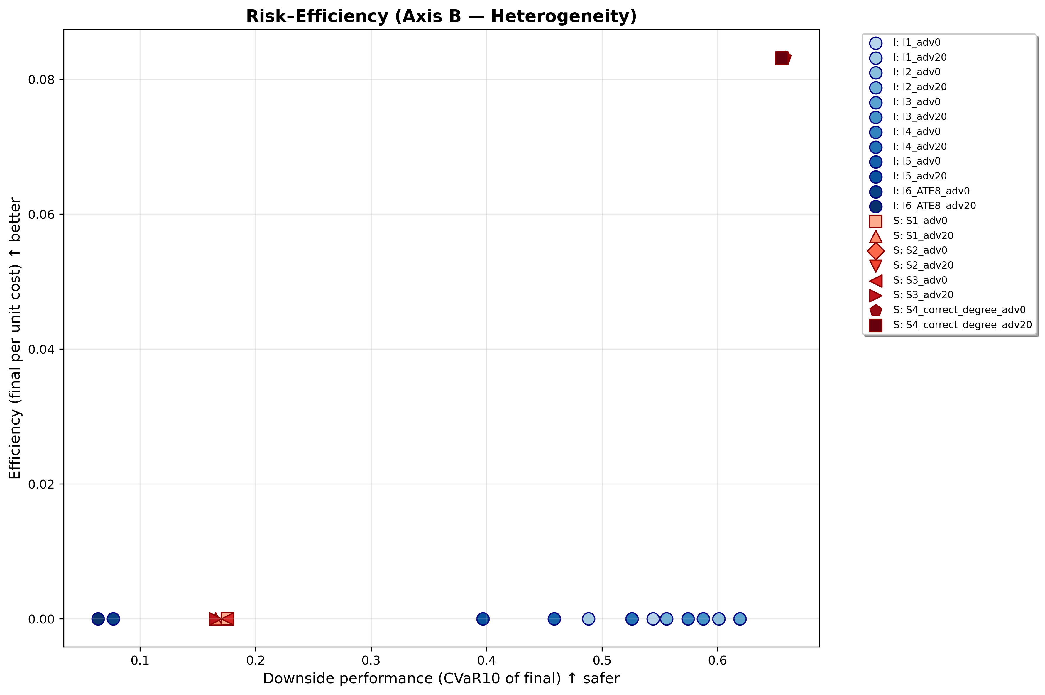
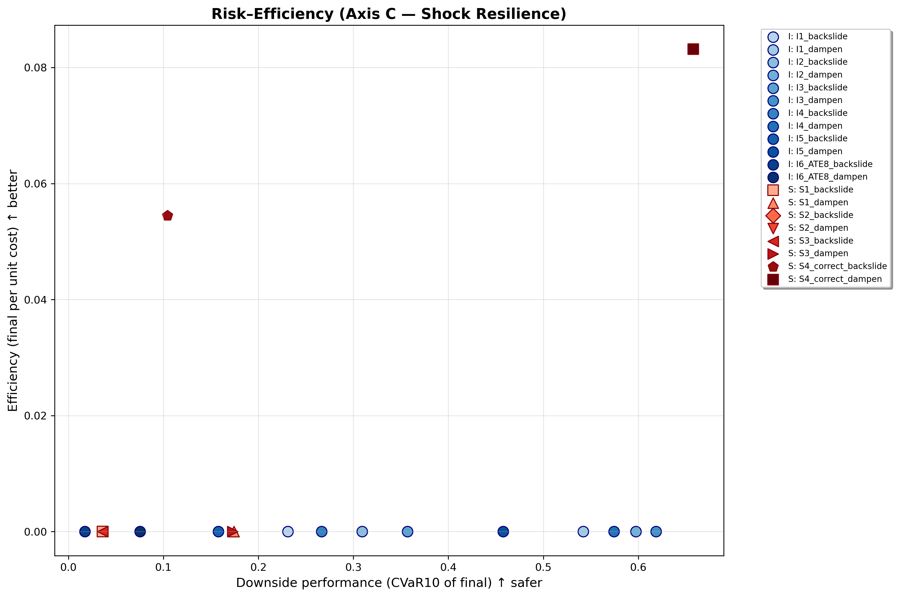
Finally, the appendix reports risk-efficiency frontiers. These plots place efficiency on the vertical axis and downside safety on the horizontal axis so that policies in the upper-right region combine stronger gains with safer worst-case performance.
Agents and dynamics
The model can be read as a simple sequence. At the start of each run, agents receive heterogeneous ceilings for how far adoption can increase, heterogeneous susceptibility to intervention, and heterogeneous social thresholds. An intervention then produces a direct gain. In the absence of reinforcement, adoption decays. For system-level interventions, neighbours can amplify gains, and once enough nearby adoption has accumulated an additional reinforcement effect can occur. Adverse response and external shocks then weaken gains or increase losses. The equations below formalise this sequence.
Each agent \(i=1,\dots,N\) has an adoption level \(A_i(t)\in[0,A^{\max}_i]\). The ceiling \(A^{\max}_i\in[0.4,0.9]\) captures heterogeneity in how far adoption can rise. Agents also differ in susceptibility \(s_i \sim U[0.5,1.5]\), which scales how strongly they respond, and in cascade threshold \(\tau_i \sim U[0.15,0.30]\), which determines how much neighbouring activation is needed before local reinforcement becomes strong. In the absence of intervention, adoption decays toward the baseline \(A_i^{\text{base}}=0\).
The population mean adoption at time \(t\) is \(\bar{A}(t)=\tfrac{1}{N}\sum_i A_i(t)\). At each step, adoption updates according to:
| \[A_i(t{+}1) = \mathrm{clip}_{[0,\,A^{\max}_i]}\Big\{A_i(t) + \mathrm{Gain}_i(t) - \delta\max\{0,\,A_i(t)-A^{\text{base}}_i\}\Big\}\] | \[(1)\] |
For i-frame interventions, the gain is:
| \[\mathrm{Gain}^{\mathrm{I}}_i(t) = s_i\, d(t)\, (A^{\max}_i - A_i(t))\] | \[(2)\] |
For s-frame interventions, the gain is:
| \[\mathrm{Gain}^{\mathrm{S}}_i(t) = s_i\, \alpha(t)\, (A^{\max}_i - A_i(t))\] | \[(3)\] |
| \[\alpha(t) = \alpha_0 + \lambda\,\bar{A}_{\mathcal{N}_i}(t) + \alpha_{\text{cascade}}\cdot\mathbf{1}\{\mathrm{cascade}_i(t)\}\] | \[(4)\] |
Here \(\bar{A}_{\mathcal{N}_i}(t)\) is mean adoption among agent \(i\)’s neighbours, \(\lambda\) is the social-reinforcement term, and \(\alpha_{\text{cascade}}\) is an additional reinforcement increment that activates when the local neighbourhood reaches a tipping point.
A cascade is therefore a local reinforcement event: enough of an agent’s neighbours have already reached relatively high adoption that diffusion becomes easier to sustain. We use a dual-gate rule,
| \[\mathrm{cascade}_i(t) = \left[\frac{\#\{j\in\mathcal{N}_i: A_j(t)\ge 0.5\}}{|\mathcal{N}_i|} \ge \tau_i\right] \;\text{or}\; \left[\#\{j\in\mathcal{N}_i: A_j(t)\ge 0.5\} \ge m\right]\] | \[(5)\] |
All updates occur in random asynchronous order at each time step: agents are randomly permuted, and each agent updates once per period.
Simulation sequence and pseudocode
The simulation sequence is straightforward. Each run begins by drawing agent attributes and constructing the relevant network information. If the scenario includes targeted seeding, the seeds are chosen before the first update. The model then iterates through time, applying intervention gains, adverse-response penalties, shocks, and decay in random asynchronous order. Algorithm 1 summarises the main simulation loop. Detailed pseudocode for the targeted seeding routine appears in Appendix A (Algorithm 2).
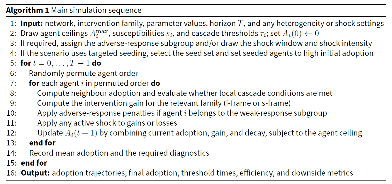
At initialization all agents start from zero adoption. In the targeted-seeding scenarios, a small number of agents are set to high adoption at \(t=0\) in order to test whether diffusion can ignite. Runs stop after the fixed horizon \(T\). Threshold times are recorded only when the corresponding threshold is actually reached.
Networks, targeting, and misspecification
The true social network \(G^{\text{true}}\) is a modular stochastic block model with equal-sized communities, within-community edge probability \(p_{\text{in}}=0.04\), between-community edge probability \(p_{\text{out}}=0.001\), and \(N=400\) nodes (Newman 2010). This creates clustered but connected social structure: targeted seeds can spread locally within communities and, if well placed, propagate across bridging ties.
To represent imperfect structural knowledge, we construct a corrupted policy network \(G^{\text{pol}}\) by rewiring edges in \(G^{\text{true}}\) with probability \(p\). Rankings based on \(G^{\text{pol}}\) need not match the truly influential nodes. This is the core manipulation in experimental dimension A.
The targeted s-frame intervention seeds \(k = \lfloor fN \rfloor\) agents at \(t=0\). When targeting is correct, nodes are ranked by degree in \(G^{\text{true}}\). Under misspecification, they are ranked by degree in \(G^{\text{pol}}\). Two additional baselines are included: purely random placement and deliberately poor placement on low-degree nodes. A clustering parameter \(q\) means that some seeds are placed near previously selected ones, which captures the fact that real implementation often concentrates activity locally rather than scattering it uniformly.
Before turning to the results, we record three placement diagnostics: overlap with the true top-\(k\) nodes, a quality ratio summarising how many high-value positions are captured, and Spearman rank correlation \(\rho\) between policy and true degree rankings (Valente 2012). These diagnostics translate the abstract idea of “structural knowledge” into quantities that could, in principle, be assessed before scaling up a targeted intervention.
Shocks, adverse response, costs, and calibration
Experimental dimension C introduces temporary disturbances. A dampening shock multiplies gains by \((1-\theta)\) during the shock window, representing a setting in which progress becomes harder but not necessarily reversible. A backsliding shock instead increases effective loss rates during the window, representing a setting in which existing adopters are more likely to revert. Shock onset is drawn from the middle portion of the policy horizon, duration is drawn from 10 to 25 periods, and intensity \(\theta\) is drawn from \([0.10,0.25]\).
Experimental dimension B introduces heterogeneous response by assigning a share \(\phi\in\{0,0.2\}\) of agents a responsiveness penalty \(\gamma\). These agents still participate in diffusion, but they convert policy exposure into adoption more weakly than the rest of the population. This captures uneven uptake without requiring a domain-specific behavioural theory for every subgroup.
Cost accounting is intentionally simple but substantively motivated. Individual interventions and mild uniform structural levers incur recurring delivery costs each period. Hub-targeted seeding incurs an upfront cost at the moment seeds are placed. The purpose is not to estimate administrative budgets in detail, but to distinguish interventions that require continuous delivery from those that rely on a concentrated initial push.
The small-effect benchmark individual intervention, I6_ATE8, is calibrated by Monte Carlo search on the true network to achieve approximately an eight-percentage-point improvement in adoption by \(T=120\), matching the scale of modest average effects often reported in the nudge literature (Della Vigna & Linos 2022; Mertens et al. 2022). The mild structural baseline S1 is tuned to remain low and non-saturating so that the targeted seeding design is not compared only against implausibly weak system alternatives.
The main text intentionally foregrounds a small set of core parameters. Table 5 summarises the defaults and their role in the model. The choices are meant to be transparent rather than optimised: the population is large enough to display meaningful network diffusion, community structure creates a realistic need for bridge placement, heterogeneous ceilings and thresholds prevent identical responses, decay makes maintenance relevant, and the small seed fraction tests whether social reinforcement can amplify a limited initial intervention.
| Component | Default specification | Interpretation | |
|---|---|---|---|
| Population and network | \(N=400\); modular stochastic block model with \(p_{\text{in}}\approx 0.04\) and \(p_{\text{out}}\approx 0.001\) | Clustered but connected social structure in which local reinforcement and bridge placement both matter. | |
| Policy horizon | \(T=80\) for network targeting experiments; \(T=120\) for heterogeneity and shock experiments | Shorter horizon for structural-information tests, longer horizon where slower adaptation and shocks matter. | |
| Agent heterogeneity | \(s_i\sim U[0.5,1.5]\); \(\tau_i\sim U[0.15,0.30]\); \(A^{\max}_i\in[0.4,0.9]\) | Agents differ in responsiveness, social threshold, and adoption ceiling. | |
| Decay | I-frame \(\delta_I\approx 0.01\); s-frame \(\delta_S\approx 0.005\); \(A_i^{\text{base}}=0\) | Adoption fades without reinforcement; system settings decay more slowly than person-level effects. | |
| Targeted seeding | Fraction \(f\approx 0.015\); seeded state \(0.90\); clustering parameter \(q\approx 0.25\) | Small initial push used to test whether local spillovers can ignite wider diffusion. | |
| Cascade rule | Fractional threshold \(\tau_i\) or at least \(m=3\) neighbours above 0.5 | Captures neighbourhood tipping without relying on only one gate. | |
| Calibration | S1 baseline strength and I6 benchmark dose calibrated on the true network | Ensures interpretable baselines rather than arbitrary magnitudes. | |
| Cost accounting | Recurring costs for I-frame and mild structural families; one-shot cost for targeted seeding | Distinguishes continuous delivery from concentrated initial placement. | |
In addition to the outcome metrics, we record target-quality diagnostics and the maximum share of agents in cascade over time. These diagnostics help connect macro outcomes back to the quality of placement and local reinforcement.
Reproducibility and robustness
Random seeds for network generation, agent attributes, and shocks are recorded per run, and update order is redrawn each period. The model was implemented in Mesa 3.2.0 (ter Hoeven et al. 2025).
Robustness checks reported in the appendix vary network structure (Watts-Strogatz and Barabási-Albert graphs) (Barabási & Albert 1999; Newman 2010; Watts & Strogatz 1998), the cascade count gate \(m\), and the social-reinforcement parameter \(\lambda\). The qualitative ordering of the main findings persists across these alternatives.
Results
The results are organised around the three experimental dimensions introduced in Table 2. Experimental dimension A concerns network information errors: it asks how much hub-targeted system intervention depends on accurate structural knowledge. Experimental dimension B concerns heterogeneous response: it asks whether weakly responsive subpopulations erode individual and system interventions in the same way. Experimental dimension C concerns shock resilience: it asks whether temporary disruptions merely slow diffusion or instead induce behavioural reversal. These dimensions correspond directly to the misspecification categories summarised in Table 1.
The figures report mean adoption trajectories with 95% confidence intervals across runs. They are complemented by the numerical summary tables in Appendix A (Tables 7, 8, 9) and by risk-efficiency frontiers in Appendix B. For readability, the prose uses descriptive names first and introduces scenario codes only where they are needed to identify a specific curve or table entry.
Across the three dimensions, a consistent pattern emerges. When system-level targeting is based on reasonably accurate structural information, it produces the fastest and most cost-efficient diffusion. When success depends on fragile local reinforcement, however, targeting errors and backsliding shocks become more damaging. Individual-level interventions remain smaller in scale, but they are also steadier and easier to predict.
Experimental dimension A: Network information errors
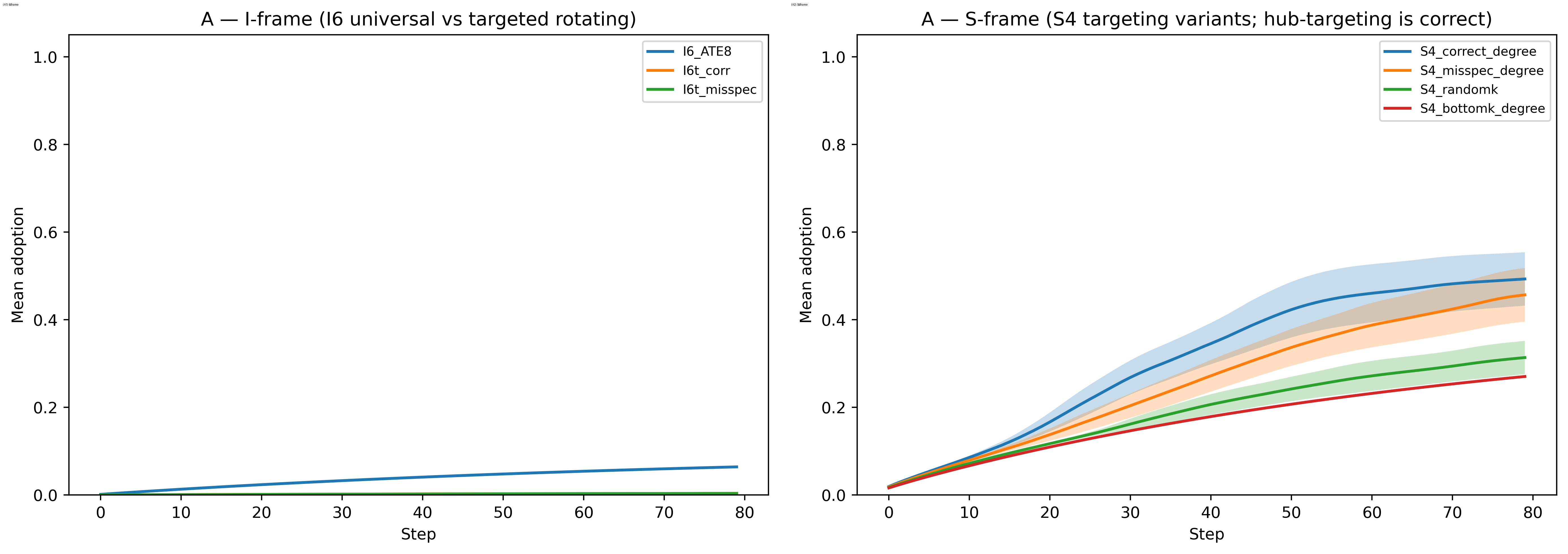
Figure 1 shows that the main advantage of targeted seeding depends on placement quality. When policymakers seed genuinely central nodes, adoption rises quickly and reaches much higher levels than the individual benchmarks. When policymakers rely on a corrupted network view, diffusion remains substantial but becomes slower and less efficient. Random placement and deliberate placement on low-value nodes perform much worse. The message is straightforward: system-level targeting can be highly effective, but it is effective conditional on usable structural knowledge. This is precisely the informational form of misspecification highlighted in the scoping review.
Experimental dimension B: heterogeneous response
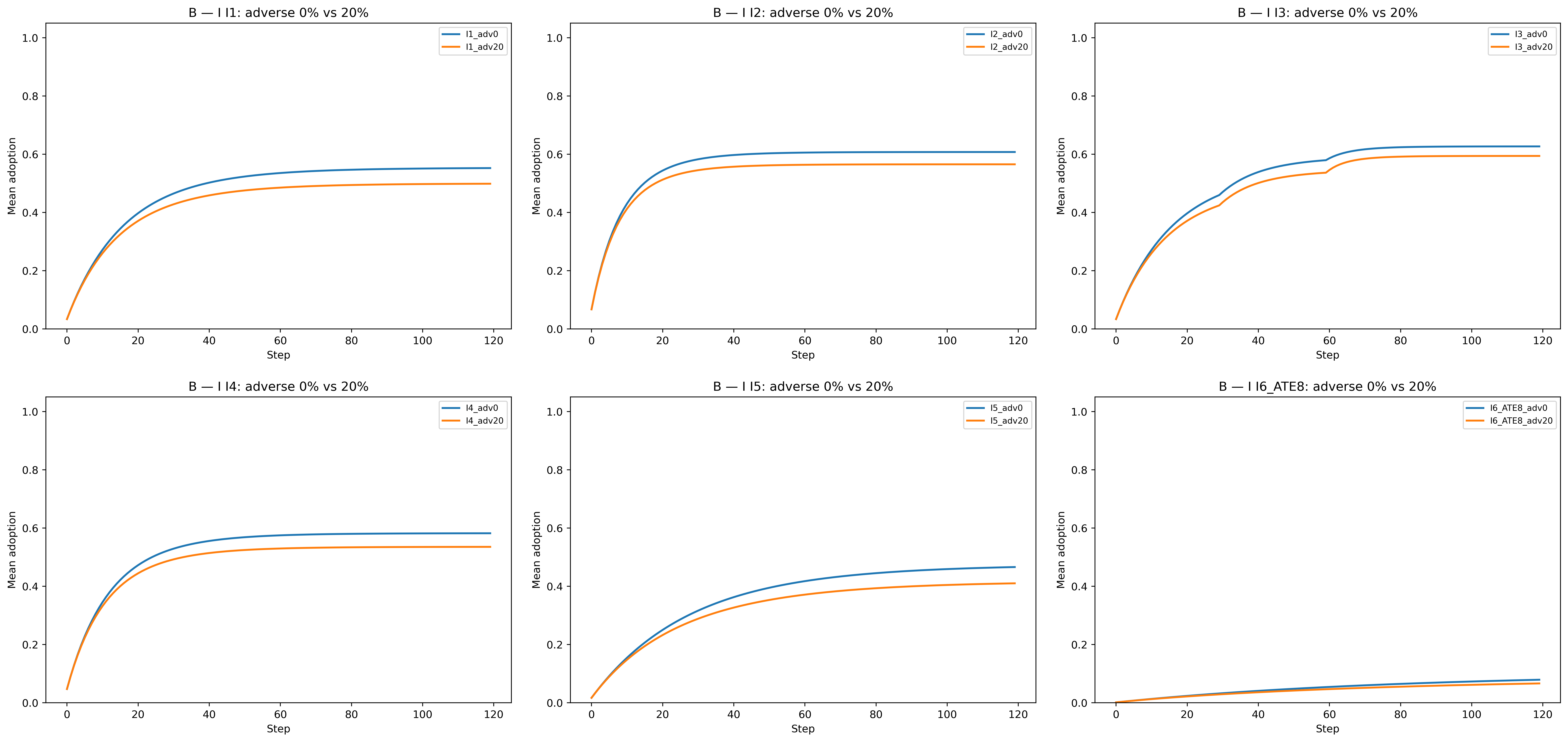
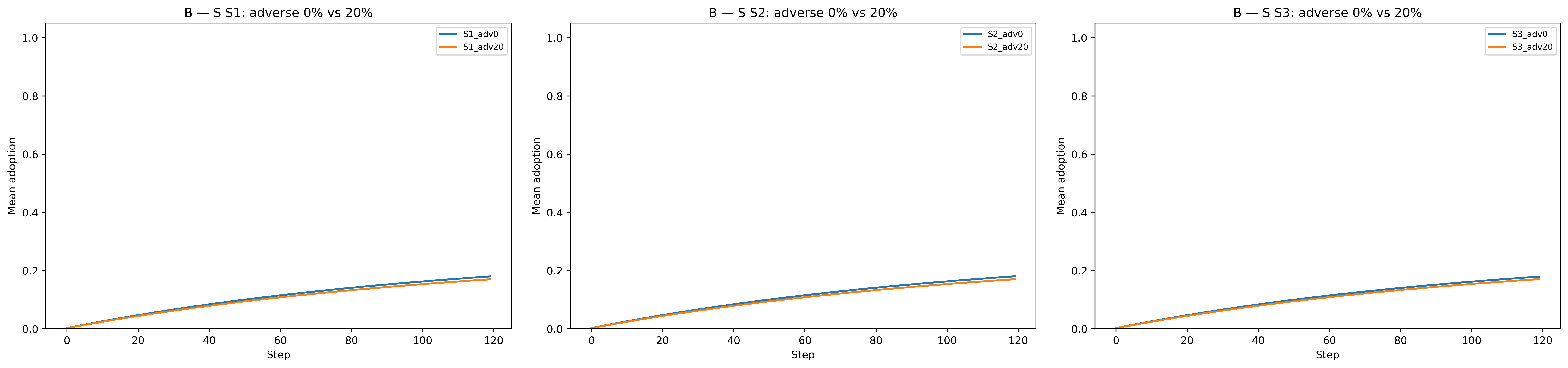
Experimental dimension B shows that weak response matters differently across intervention families. The individual-level families shift downward when 20% of the population responds weakly: adoption rises more slowly and ends at lower levels. The mild uniform structural levers remain low in both conditions. By contrast, hub-targeted seeding changes relatively little at the parameter values studied. Once well-placed seeds have activated neighbourhood reinforcement, some of the burden of change is carried by local spillovers rather than by repeated direct treatment of each individual. In substantive terms, this means that heterogeneous response can erode individual interventions directly, whereas system interventions can sometimes buffer it through social reinforcement.
Experimental dimension C: shock resilience
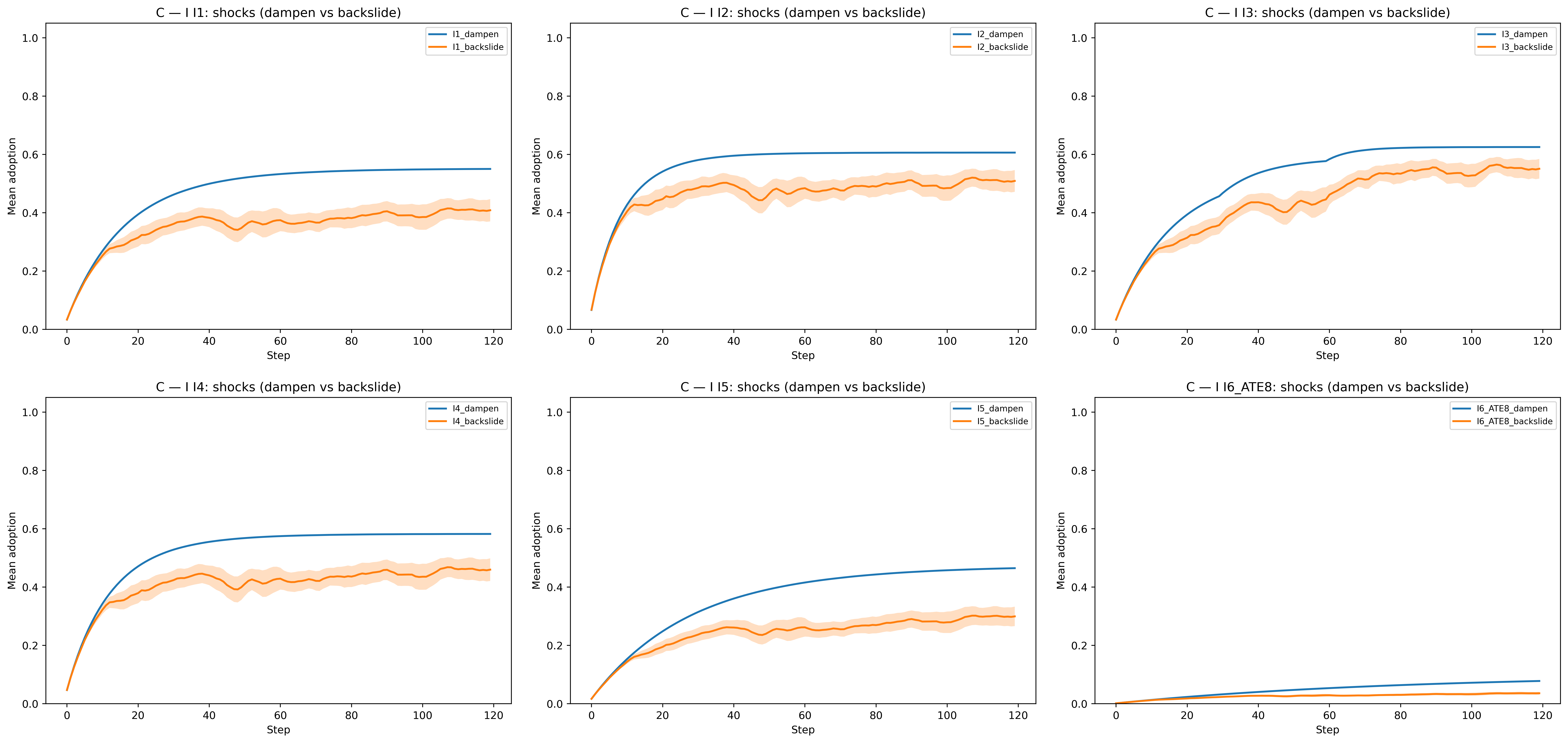
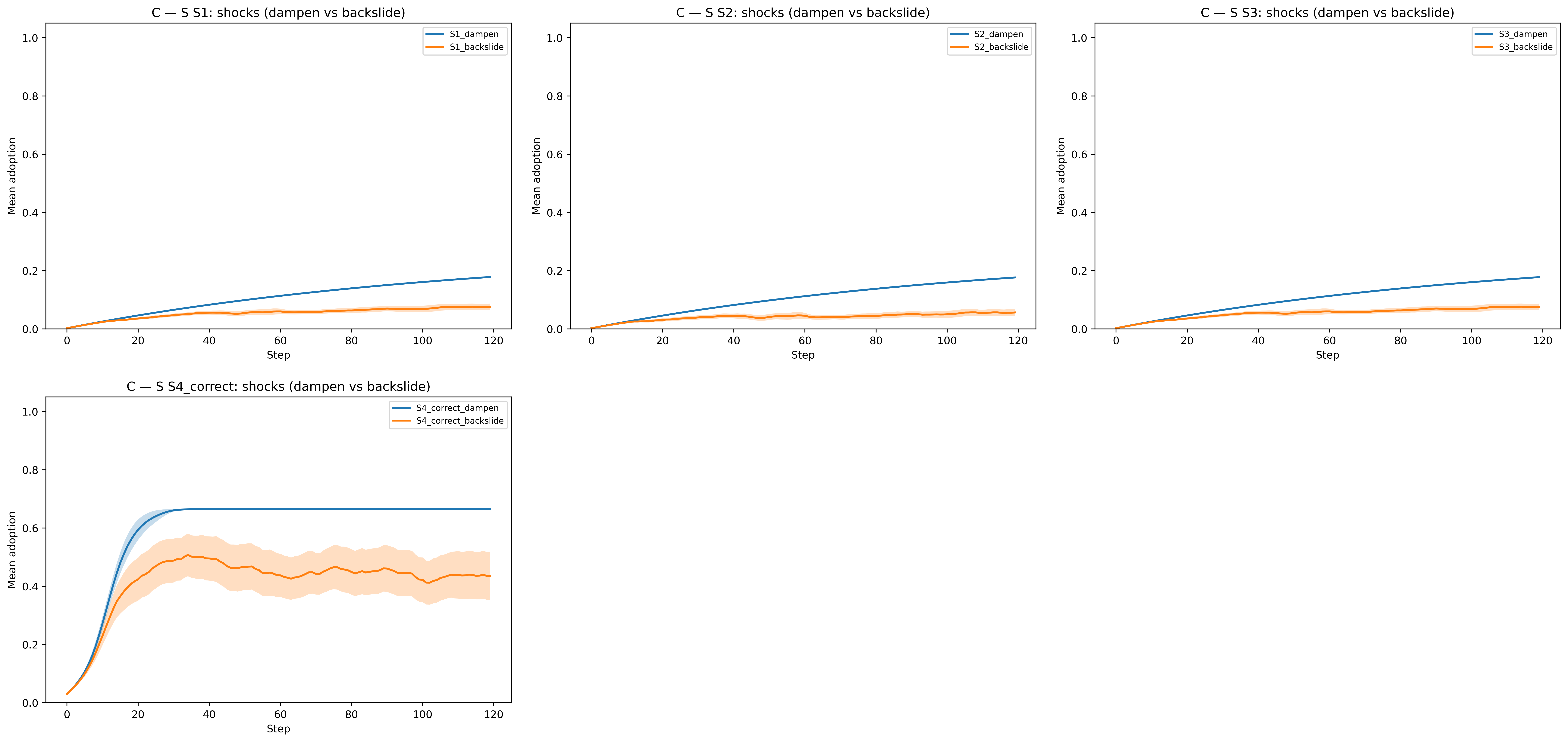
The shock experiments reveal a more asymmetric pattern. Dampening shocks mainly slow diffusion: they postpone gains but do not fundamentally alter the ranking of interventions. Backsliding shocks are more consequential. They reduce the performance of individual interventions, but they are especially damaging for system-level diffusion that depends on neighbourhoods remaining above local reinforcement thresholds. When backsliding pushes enough agents below those thresholds, the self-reinforcing logic that made targeted seeding powerful becomes a source of fragility. The numerical summaries in Table 9and the risk-efficiency frontier in Appendix B (Figure 8) make this shift visible.
Discussion
The paper set out to clarify a question that is often implied but rarely formalised in the i-/s-frame debate: are system-level interventions preferable because they can produce larger change, or do the conditions that make them powerful also make them more fragile? The simulations suggest that both claims are true, depending on the form of misspecification. In other words, the relevant comparison is not simply “larger effects” versus “smaller effects.” It is a comparison between transformation and robustness.
Taken together, the scoping review and the model show that system-level interventions are most attractive when policymakers have usable structural information and when the surrounding environment is stable enough for local reinforcement to accumulate. Under those conditions, targeted seeding can convert a small initial intervention into a much larger population effect. The same dependence on social reinforcement, however, makes system-level diffusion more exposed to certain kinds of error and instability than person-level interventions are.
What the three experimental dimensions show
Network information errors. Experimental dimension A translates the scoping review’s informational and institutional concerns into a direct targeting problem. When influential nodes are identified reasonably well, targeted seeding is both fast and cost-efficient. When policymakers target using corrupted structural information, the intervention still works, but it works more slowly and less efficiently. Random or low-value placement performs markedly worse. The substantive implication is that structural information is not a minor implementation detail. For targeted system intervention, it is a first-order input. Read against the network-intervention literature, this sharpens a point already implicit in arguments that placement within social structure can decisively shape intervention performance (Centola 2018; Valente 2012). It also aligns with field evidence that injection points and network-informed targeting can materially alter population-level diffusion outcomes (Airoldi & Christakis 2024; Banerjee et al. 2013; Kim et al. 2015). Our contribution is to show that the same dependence on placement quality is also a source of policy vulnerability: errors in structural knowledge degrade system-level strategies more sharply than they degrade person-level benchmarks.
Heterogeneous response. Experimental dimension B shows that weak response harms intervention families differently. Individual-level interventions depend heavily on repeated direct gains to the treated person, so a sizeable weak-response subgroup lowers both speed and final adoption. The well-targeted seeding design is less affected because some of the work of diffusion is shifted from repeated direct treatment to social reinforcement among neighbours. This does not mean that system interventions are generally immune to heterogeneity. It means that heterogeneity matters through a different pathway when diffusion is sustained by local spillovers. This speaks to evidence that choice-architecture and nudge interventions often generate positive but modest average effects, especially at scale and across heterogeneous settings (Beshears & Kosowsky 2020; Della Vigna & Linos 2022; Mertens et al. 2022). The present results add a mechanism-level interpretation: when response is uneven, person-level treatment may remain bounded unless local reinforcement amplifies change (Centola 2018; Centola & Macy 2007).
Shock resilience. Experimental dimension C is the clearest illustration of the transformation-robustness trade-off. Temporary dampening mainly slows diffusion for both families. Backsliding shocks are different because they threaten the persistence of already-achieved adoption. The targeted seeding design loses more under these conditions because it relies on neighbourhoods staying above local reinforcement thresholds. Individual-level interventions deliver smaller gains, but their logic does not depend on maintaining the same kind of network-driven momentum. In that sense, the results bring threshold and cascade models (Granovetter 1978; Watts 2002) into direct conversation with policy literatures on uncertainty, turbulence, and instability (Cairney 2012; Geyer & Cairney 2015; Head 2008; Room 2011): the same local reinforcement that enables large gains also makes diffusion more sensitive to reversals that push neighbourhoods below activation thresholds.
A brief note on cost accounting is warranted because cost-efficiency is central to the argument. The model compares recurrent delivery costs for person-level interventions and mild uniform structural levers with an upfront cost for targeted seeding. This distinction is substantively motivated: many behavioural campaigns require continuous outreach, whereas seeding-style interventions often concentrate effort early. The results should therefore be interpreted as showing that spillovers can make an upfront intervention highly productive when targeting is good, not that all system interventions are universally cheap. This reading is also consistent with implementation scholarship emphasising that delivery burdens and administrative demands shape realised policy performance (Moynihan et al. 2015; Pressman & Wildavsky 1973), and with network-intervention work showing that strategic placement can substitute for repeated blanket contact (Valente 2012).
Implications for policy design and empirical research
For policy design, the main implication is that structural knowledge should be treated as a practical precondition for scaling system-level targeting. Before a policy relies on hub targeting or other network-sensitive mechanisms, policymakers need evidence that the network information they hold is good enough for the intervention logic they propose. In applied settings, this means measuring not only whether an intervention can work in principle, but whether the available information is sufficient to place it effectively, a lesson consistent with network-targeting field studies (Airoldi & Christakis 2024; Kim et al. 2015).
A second implication is that uncertainty should change how system interventions are deployed. The results support a staged approach rather than an all-or-nothing choice. When structural information is good and external disruption is limited, system-level intervention can justifiably be used more aggressively. When information is weak or backsliding is plausible, a more cautious design is warranted: pilot placement, learn before scaling, and pair system-level measures with steadier person-level components that provide a floor while knowledge improves (Cairney 2012; Geyer & Cairney 2015; Haynes et al. 2012; Room 2011).
The model also generates empirical propositions. Field studies could examine whether targeting quality predicts diffusion success when system interventions rely on social structure, building on experimental designs that vary injection points or targeting algorithms in real networks (Airoldi & Christakis 2024; Banerjee et al. 2013; Kim et al. 2015). Comparative policy analyses could test whether system-level interventions exhibit greater cross-context variance than person-level ones. Natural experiments around crises or competing campaigns could examine whether network-dependent policies are disproportionately vulnerable to behavioural backsliding. These are feasible ways to move from a mechanism-oriented model toward empirically grounded comparative evidence.
Limitations and future research
The first limitation is that networks are held fixed over the policy horizon. In reality, social ties can change as adoption spreads, and policies can themselves alter the structure through which later influence travels. Relatedly, the model does not capture meso-level drivers of behavioural adaptation such as dynamic network externalities, changing local norms, or shifting payoffs as adoption accumulates. Recent network-targeting field studies suggest that these meso-level dynamics are empirically consequential, not merely theoretical (Airoldi & Christakis 2024; Kim et al. 2015). Complexity-oriented policy scholarship argues that effective public policy often works by creating conditions for adaptive, pro-social network externalities rather than by acting only on isolated individuals (Cairney 2012; Colander & Kupers 2014; Geyer & Cairney 2015; Room 2011). Extending the model to co-evolving networks and endogenous externalities is therefore an important next step.
A second limitation is cognitive and organisational simplicity. Agents do not learn, reinterpret the intervention, or strategically adapt to it, and policymakers do not monitor results and retarget in real time. The model therefore captures one important aspect of social diffusion – local reinforcement – but not the full interpretive, strategic, or administrative complexity of real implementation, themes that are central in the implementation literature (Matland 1995; McConnell 2014; Pressman & Wildavsky 1973).
A third limitation concerns abstraction. Costs are stylised rather than administratively detailed, heterogeneous response is represented in reduced form, and the model focuses on aggregate adoption rather than on distributional outcomes. It therefore cannot tell us who benefits first, who bears downside risk, or how political transaction costs alter the attractiveness of different policy bundles. These omissions matter because distributional burdens and administrative frictions are often decisive in real policy evaluation (Della Vigna & Linos 2022; Moynihan et al. 2015).
Finally, downside risk is summarised partly through a 10% failure-to-diffuse threshold. That cutoff is useful for comparative purposes, but it will not be substantively appropriate in every policy domain. For that reason, the analysis also reports \(\mathrm{CVaR}_{10}\) and interprets conclusions in terms of the broader ranking of intervention families rather than one threshold alone.
Taken together, these limitations do not undermine the main contribution. They locate it more precisely: the paper offers a transparent comparative framework for thinking about when larger system effects are worth the added exposure to misspecification, and which forms of uncertainty are most consequential for that judgement. In that sense, the model serves the clarifying role of a mechanism-oriented comparative exposition: it makes the conditional trade-offs visible before they are tested in richer empirical settings (Edmonds et al. 2019; Epstein 2008).
Conclusions
This paper revisits the i-/s-frame debate (Chater & Loewenstein 2022) by asking a narrower and more operational question than the debate is usually asked in prose: how do individual-level and system-level interventions compare once misspecification risk is made explicit? The answer is not that one family is always better. It is that they solve different problems under different informational and environmental conditions.
System-level interventions can deliver much larger and more cost-efficient gains when they are well aligned with the social structure through which influence travels (Centola 2018; Chater & Loewenstein 2022; Valente 2012). In the model, a small number of well-placed seeds can trigger broader diffusion that no similarly modest person-level benchmark can match, echoing work on network interventions and injection-point selection (Airoldi & Christakis 2024; Banerjee et al. 2013; Kim et al. 2015). This is the main source of their transformative promise.
The same result also explains their fragility. When policymakers target the wrong parts of the network, or when external conditions make already-achieved adoption harder to maintain, system-level diffusion loses momentum more quickly. Individual-level interventions usually do less, but they also fail in smaller and more predictable ways, a pattern consistent with evidence that many choice-architecture and information interventions produce positive but comparatively modest effects at scale (Beshears & Kosowsky 2020; Della Vigna & Linos 2022; Mertens et al. 2022), even as critics note their limited capacity to address structurally generated problems (Chater & Loewenstein 2022). The central policy trade-off is therefore between the scale of possible gains and the robustness of those gains to misspecification.
The practical implication is not to choose once and for all between person-level and system-level policy. It is to sequence and combine them more intelligently. System-level interventions are most defensible when structural knowledge is good, the implementation environment is sufficiently stable, and policymakers are willing to learn before scaling. Individual-level interventions remain valuable as steadier background measures and as safeguards when uncertainty is high. Future work should extend this comparison to dynamic networks, richer behavioural adaptation, and distributional outcomes so that the transformation–robustness trade-off can be assessed in more realistic policy settings. More broadly, the paper’s methodological contribution is to show that an ABM framework for comparing intervention families provides a cumulative way to incorporate precisely those advances—dynamic networks, adaptation, and richer contexts—without losing sight of the original i-/s-frame policy question (Edmonds et al. 2019; Epstein 2008). In that sense, the framework is valuable not only because it compares existing intervention logics, but also because it provides a disciplined way to extend that comparison as the surrounding literatures advance.
Model Documentation
The model was developed using the Python library Mesa 3.2.0 (ter Hoeven et al. 2025). Documentation and the code in the format of an annotated Jupyter notebook are available here: https://osf.io/4zexa/overview?view_only=ae3db91b10d7427ea9aa01d4962bfea9. The repository includes extensive inline documentation for replication and inspection.Funding
The authors have not received specific funds for this work.Conflict of Interest
The authors declare no conflict of interest.Ethics Approval
Not applicable, use of synthetic data.Consent to Participate
Not applicable, use of synthetic data.Appendix A: Parameters and Implementation
| Population and network | \(N=400\); modular SBM (\(p_{\text{in}}\approx 0.04\), \(p_{\text{out}}\approx 0.001\)) |
| Activation and horizon | Random agent activation; \(T \in \{80,120\}\) depending on the experimental dimension |
| Heterogeneity | \(s_i\sim U[0.5,1.5]\); \(\tau_i\sim U[0.15,0.30]\); \(A^{\max}_i\in[0.4,0.9]\) |
| Decay | I: \(\delta_I\approx 0.01\); S: \(\delta_S\approx 0.005\); \(A^{\text{base}}_i=0\) |
| S4 targeting | fraction \(f\approx 0.015\); seed-to-state level \(0.90\); cluster prob \(q\approx 0.25\) |
| Cascade gate | fraction threshold \(\tau_i\) or \(\ge m\) contacts above \(0.5\) (experimental dimension A: \(m{=}3\)) |
| Calibration | S1 baseline \(\alpha_0\) and I6_ATE8 dose via Monte-Carlo on the actual graph |
| Costs | I: per-step delivery; S1/S3: per-step; S4: one-shot seeding at \(t=0\) |
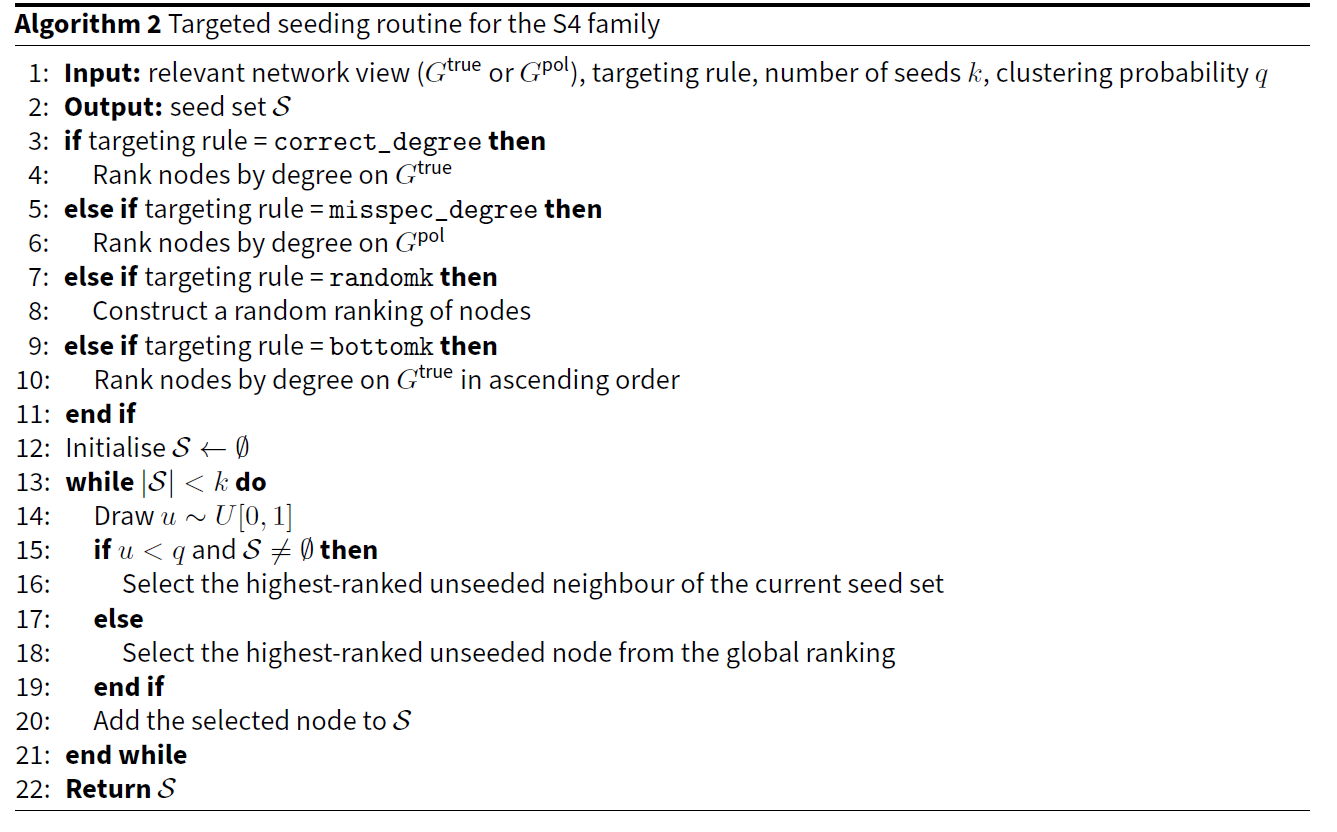
Detailed targeted-seeding routine. The targeted seeding logic used by the S4 family is reported here because it is important for replication but not necessary for following the main argument in the body of the paper.
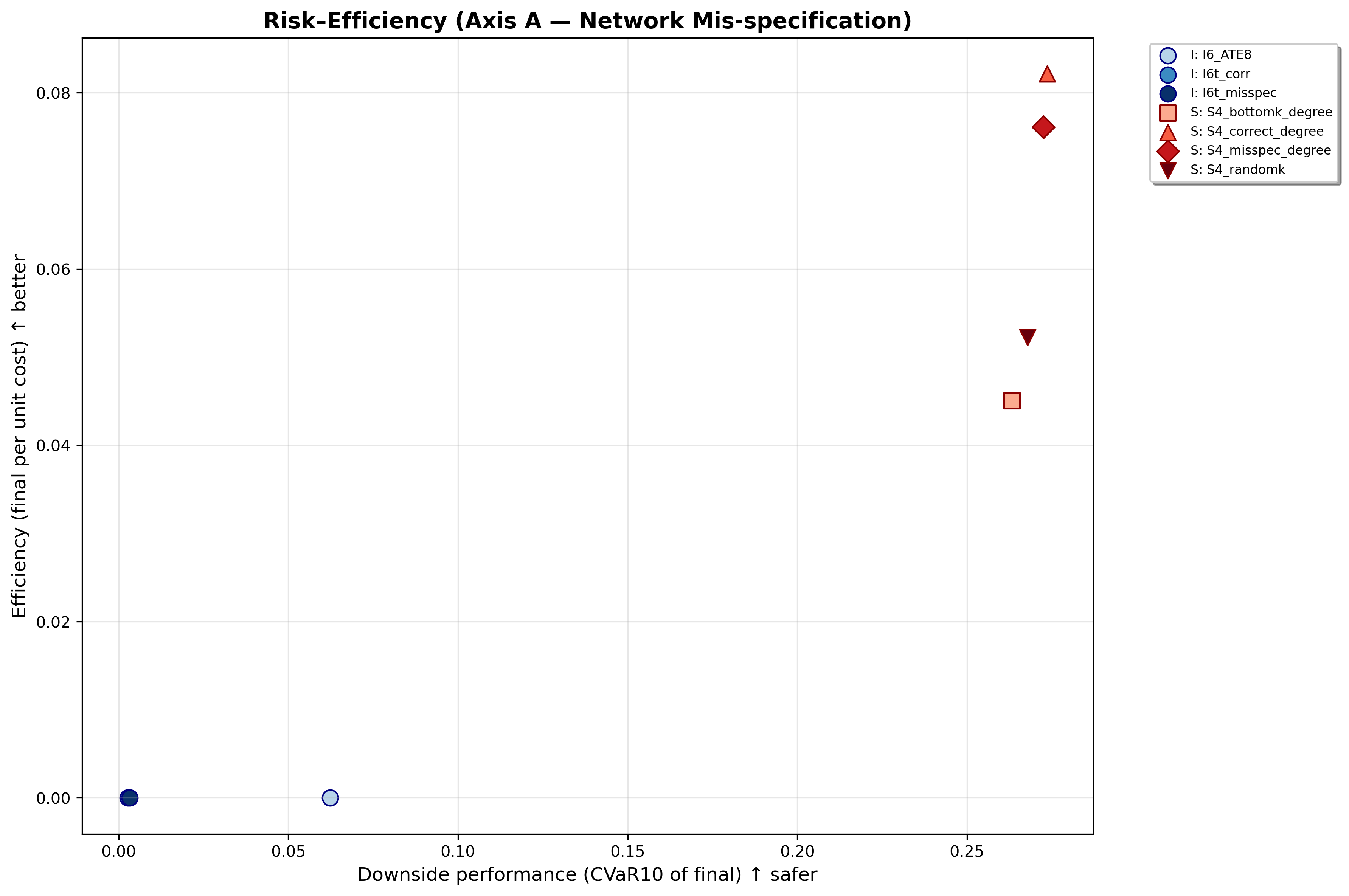
| Scenario | Final | t50 | Eff(final) | Eff(AUC) | CVaR10 | Catastrophe (%) |
|---|---|---|---|---|---|---|
| S4_correct_degree | 0.493 | 45.500 | 8.21e-02 | 5.14e-02 | 0.274 | 0.0 |
| S4_misspec_degree | 0.457 | 63.000 | 7.61e-02 | 4.29e-02 | 0.273 | 0.0 |
| S4_randomk | 0.313 | 60.000 | 5.22e-02 | 3.17e-02 | 0.268 | 0.0 |
| S4_bottomk_degree | 0.270 | — | 4.50e-02 | 2.77e-02 | 0.263 | 0.0 |
| I6_ATE8 | 0.064 | — | 1.92e-06 | 1.14e-06 | 0.062 | 100.0 |
| I6t_corr | 0.003 | — | 1.93e-06 | 1.14e-06 | 0.003 | 100.0 |
| I6t_misspec | 0.003 | — | 1.99e-06 | 1.14e-06 | 0.003 | 100.0 |
| Scenario | Final | t50 | Eff(final) | Eff(AUC) | CVaR10 | Catastrophe (%) |
|---|---|---|---|---|---|---|
| I1_adv0 | 0.552 | 40.000 | 1.15e-05 | 9.95e-06 | 0.544 | 0.0 |
| I1_adv20 | 0.499 | 87.000 | 1.04e-05 | 9.07e-06 | 0.488 | 0.0 |
| I2_adv0 | 0.607 | 16.000 | 1.26e-05 | 1.17e-05 | 0.599 | 0.0 |
| I2_adv20 | 0.574 | 17.000 | 1.19e-05 | 1.10e-05 | 0.566 | 0.0 |
| I3_adv0 | 0.628 | 34.000 | 1.30e-05 | 1.21e-05 | 0.620 | 0.0 |
| I3_adv20 | 0.596 | 41.000 | 1.24e-05 | 1.15e-05 | 0.588 | 0.0 |
| I4_adv0 | 0.582 | 24.000 | 1.20e-05 | 1.10e-05 | 0.575 | 0.0 |
| I4_adv20 | 0.549 | 25.000 | 1.13e-05 | 1.03e-05 | 0.543 | 0.0 |
| I5_adv0 | 0.464 | — | 9.57e-06 | 8.05e-06 | 0.456 | 0.0 |
| I5_adv20 | 0.422 | — | 8.82e-06 | 7.39e-06 | 0.404 | 0.0 |
| I6_ATE8_adv0 | 0.063 | — | 1.88e-06 | 1.12e-06 | 0.061 | 100.0 |
| I6_ATE8_adv20 | 0.058 | — | 1.74e-06 | 1.06e-06 | 0.056 | 100.0 |
| S1_adv0 | 0.198 | — | 1.10e-05 | 6.36e-06 | 0.194 | 0.0 |
| S1_adv20 | 0.187 | — | 1.04e-05 | 6.00e-06 | 0.181 | 0.0 |
| S2_adv0 | 0.181 | — | 1.00e-05 | 5.78e-06 | 0.176 | 0.0 |
| S2_adv20 | 0.170 | — | 9.39e-06 | 5.47e-06 | 0.166 | 0.0 |
| S3_adv0 | 0.175 | — | 9.67e-06 | 5.60e-06 | 0.170 | 0.0 |
| S3_adv20 | 0.165 | — | 9.12e-06 | 5.30e-06 | 0.160 | 0.0 |
| S4_correct_degree_adv0 | 0.666 | 16.000 | 8.33e-02 | 7.51e-02 | 0.659 | 0.0 |
| S4_correct_degree_adv20 | 0.665 | 18.000 | 8.31e-02 | 7.40e-02 | 0.656 | 0.0 |
| Scenario | Final | t50 | Eff(final) | Eff(AUC) | CVaR10 | Catastrophe (%) |
|---|---|---|---|---|---|---|
| I1_dampen | 0.550 | 40.500 | 1.15e-05 | 9.89e-06 | 0.542 | 0.0 |
| I1_backslide | 0.408 | 79.500 | 8.51e-06 | 7.31e-06 | 0.231 | 0.0 |
| I2_dampen | 0.606 | 15.500 | 1.26e-05 | 1.17e-05 | 0.597 | 0.0 |
| I2_backslide | 0.503 | 16.500 | 1.05e-05 | 9.06e-06 | 0.293 | 0.0 |
| I3_dampen | 0.628 | 34.000 | 1.30e-05 | 1.21e-05 | 0.619 | 0.0 |
| I3_backslide | 0.573 | — | 1.19e-05 | 1.09e-05 | 0.311 | 0.0 |
| I4_dampen | 0.582 | 24.000 | 1.20e-05 | 1.10e-05 | 0.575 | 0.0 |
| I4_backslide | 0.458 | 31.000 | 9.45e-06 | 8.25e-06 | 0.252 | 0.0 |
| I5_dampen | 0.464 | — | 9.58e-06 | 8.05e-06 | 0.460 | 0.0 |
| I5_backslide | 0.300 | — | 6.20e-06 | 4.64e-06 | 0.146 | 0.0 |
| I6_ATE8_dampen | 0.064 | — | 1.83e-06 | 1.12e-06 | 0.062 | 100.0 |
| I6_ATE8_backslide | 0.037 | — | 1.06e-06 | 7.81e-07 | 0.017 | 100.0 |
| S1_dampen | 0.198 | — | 1.10e-05 | 6.36e-06 | 0.194 | 0.0 |
| S1_backslide | 0.050 | — | 2.77e-06 | 2.03e-06 | 0.024 | 93.3 |
| S2_dampen | 0.181 | — | 9.98e-06 | 5.80e-06 | 0.177 | 0.0 |
| S2_backslide | 0.056 | — | 3.06e-06 | 2.33e-06 | 0.026 | 83.3 |
| S3_dampen | 0.175 | — | 9.58e-06 | 5.79e-06 | 0.171 | 0.0 |
| S3_backslide | 0.076 | — | 1.58e-06 | 1.13e-06 | 0.036 | 76.7 |
| S4_correct_dampen | 0.665 | 16.000 | 8.32e-02 | 7.47e-02 | 0.658 | 0.0 |
| S4_correct_backslide | 0.436 | 17.000 | 5.45e-02 | 5.19e-02 | 0.104 | 3.3 |
Appendix B: Additional Figures, Risk-Efficiency Frontiers
The following figures display the risk-efficiency trade-off for each experimental dimension. In each plot, the vertical axis shows efficiency (final adoption per unit cost; higher is better) and the horizontal axis shows downside safety measured by CVaR\(_{10}\) (the average final adoption in the worst 10% of runs; higher is safer). Interventions closer to the upper-right corner combine stronger gains with safer downside performance.
References
ADAMS, J., Mytton, O., White, M., & Monsivais, P. (2016). Why are some population interventions for diet and obesity more equitable and effective than others? The role of individual agency. PLoS Medicine, 13(4), e1001990. [doi:10.1371/journal.pmed.1001990]
AIROLDI, E. M., & Christakis, N. A. (2024). Induction of social contagion for diverse outcomes in structured experiments in isolated villages. Science, 384(6695), eadi5147. [doi:10.1126/science.adi5147]
ARKSEY, H., & O’Malley, L. (2005). Scoping studies: Towards a methodological framework. International Journal of Social Research Methodology, 8(1), 19–32. [doi:10.1080/1364557032000119616]
ARTHUR, W. B. (1989). Competing technologies, increasing returns, and lock-in by historical events. The Economic Journal, 99(394), 116–131. [doi:10.2307/2234208]
BANERJEE, A., Chandrasekhar, A. G., Duflo, E., & Jackson, M. O. (2013). The diffusion of microfinance. Science, 341(6144), 1236498. [doi:10.1126/science.1236498]
BARABÁSI, A.-L., & Albert, R. (1999). Emergence of scaling in random networks. Science, 286(5439), 509–512.
BERRY, F. S., & BERRY, W. D. (1990). State lottery adoptions as policy innovations: An event history analysis. American Political Science Review, 84(2), 395–415. [doi:10.2307/1963526]
BESHEARS, J., & Kosowsky, H. (2020). Nudging: Progress to date and future directions. Organizational Behavior and Human Decision Processes, 161, 3–19. [doi:10.1016/j.obhdp.2020.09.001]
CAIRNEY, P. (2012). Complexity theory in political science and public policy. Political Studies Review, 10(3), 346–358. [doi:10.1111/j.1478-9302.2012.00270.x]
CENTOLA, D. (2018). How Behavior Spreads: The Science of Complex Contagions. Princeton, NJ: Princeton University Press.
CENTOLA, D., & Macy, M. (2007). Complex contagions and the weakness of long ties. American Journal of Sociology, 113(3), 702–734. [doi:10.1086/521848]
CHATER, N., & Loewenstein, G. (2022). The i-frame and the s-frame: How focusing on individual-level solutions has led behavioral public policy astray. Behavioral and Brain Sciences, 46, e147. [doi:10.1017/s0140525x22002023]
COLANDER, D., & Kupers, R. (2014). Complexity and the Art of Public Policy: Solving Society’s Problems from the Bottom Up. Princeton, NJ: Princeton University Press.
COLEMAN, J. S. (1990). Foundations of Social Theory. Cambridge, MA: Harvard University Press.
CONNOLLY, D. J., Loewenstein, G., & Chater, N. (2025). An s-frame agenda for behavioral public policy research. Behavioural Public Policy, 9(3), 593–613. [doi:10.1017/bpp.2024.58]
DELLA Vigna, S., & Linos, E. (2022). RCTs to scale: Comprehensive evidence from two nudge units. The Quarterly Journal of Economics, 137(4), 2305–2348. [doi:10.3386/w27594]
EDMONDS, B., Le Page, C., Bithell, M., Chattoe-Brown, E., Grimm, V., Meyer, R., Montañola-Sales, C., Ormerod, P., Root, H., & Squazzoni, F. (2019). Different modelling purposes. Journal of Artificial Societies and Social Simulation, 22(3), 6. [doi:10.18564/jasss.3993]
EPSTEIN, J. M. (2008). Why model? Journal of Artificial Societies and Social Simulation, 11(4), 12.
FLYVBJERG, B. (2009). Survival of the unfittest: Why the worst infrastructure gets built—and what we can do about it. Oxford Review of Economic Policy, 25(3), 344–367. [doi:10.1093/oxrep/grp024]
GEYER, R., & Cairney, P. (2015). Handbook on Complexity and Public Policy. Cheltenham: Edward Elgar.
GRANOVETTER, M. (1978). Threshold models of collective behavior. American Journal of Sociology, 83(6), 1420–1443. [doi:10.1086/226707]
HAYNES, L., Service, O., Goldacre, B., & Torgerson, D. (2012). Test, learn, adapt: Developing public policy with randomised controlled trials. [doi:10.2139/ssrn.2131581]
HEAD, B. W. (2008). Wicked problems in public policy. Australian Journal of Public Administration, 67(4), 441–450.
HOWLETT, M. (2012). The lessons of failure: Learning and blame avoidance in public policy-making. International Political Science Review, 33(5), 539–555. [doi:10.1177/0192512112453603]
LORENC, T., Petticrew, M., Welch, V., & Tugwell, P. (2013). What types of interventions generate inequalities? Evidence from systematic reviews. Journal of Epidemiology and Community Health, 67(2), 190–193. [doi:10.1136/jech-2012-201257]
MATLAND, R. E. (1995). Synthesizing the implementation literature: The ambiguity-conflict model of policy implementation. Journal of Public Administration Research and Theory, 5(2), 145–174.
MCCONNELL, A. (2010). Policy success, policy failure and grey areas in-between. Journal of Public Policy, 30(3), 345–362. [doi:10.1017/s0143814x10000152]
MCCONNELL, A. (2014). Two orders of governance failure: Design mismatches and policy–implementation gaps. Policy & Society, 33(4), 317–327.
MERTENS, S., Herberz, M., Hahnel, U. J. J., & Brosch, T. (2022). The effectiveness of nudging: A meta-analysis of choice architecture interventions across behavioral domains. Proceedings of the National Academy of Sciences, 119(1), e2107346118. [doi:10.1073/pnas.2107346118]
MOYNIHAN, D. P., Herd, P., & Harvey, T. (2015). Administrative burden: Learning, psychological, and compliance costs in citizen–state interactions. Journal of Public Administration Research and Theory, 25(1), 43–69. [doi:10.1093/jopart/muu009]
NEWMAN, M. E. J. (2010). Networks: An Introduction. Oxford: Oxford University Press.
PIERSON, P. (2000). Increasing returns, path dependence, and the study of politics. American Political Science Review, 94(2), 251–267. [doi:10.2307/2586011]
PRESSMAN, J. L., & Wildavsky, A. (1973). Implementation: How Great Expectations in Washington are Dashed in Oakland. Berkeley, CA: University of California Press.
RITTEL, H. W. J., & Webber, M. M. (1973). Dilemmas in a general theory of planning. Policy Sciences, 4(2), 155–169. [doi:10.1007/bf01405730]
ROOM, G. (2011). Complexity, Institutions and Public Policy: Agile Decision-Making in a Turbulent World. Cheltenham: Edward Elgar.
SABATIER, P. A., & Mazmanian, D. (1980). The implementation of public policy: A framework of analysis. Policy Studies Journal, 8(4), 538–560. [doi:10.1111/j.1541-0072.1980.tb01266.x]
SHIPAN, C. R., & Volden, C. (2008). The mechanisms of policy diffusion. American Journal of Political Science, 52(4), 840–857. [doi:10.1111/j.1540-5907.2008.00346.x]
TER Hoeven, E., Kwakkel, J., Hess, V., Pike, T., Wang, B., rht, & Kazil, J. (2025). Mesa 3: Agent-based modeling with Python in 2025. Journal of Open Source Software, 10(107), 7668. [doi:10.21105/joss.07668]
VALENTE, T. W. (2012). Network interventions. Science, 337(6090), 49–53.
WALKER, J. L. (1969). The diffusion of innovations among the american states. American Political Science Review, 63(3), 880–899. [doi:10.2307/1954434]
WATTS, D. J. (2002). A simple model of global cascades on random networks. Proceedings of the National Academy of Sciences, 99(9), 5766–5771. [doi:10.1073/pnas.082090499]
WATTS, D. J., & Strogatz, S. H. (1998). Collective dynamics of “small-world” networks. Nature, 393(6684), 440–442. [doi:10.1038/30918]