From Population Diversity to Contact Diversity: A Network-Based Generalization of the Greenberg Index

Université de Genève, Switzerland
Journal of Artificial
Societies and Social Simulation 29 (4) 1
<https://www.jasss.org/29/4/1.html>
DOI: 10.18564/jasss.6155
Received: 28-Mar-2026 Accepted: 19-Jul-2026 Published: 31-Oct-2026
Abstract
Quantifying linguistic diversity is central to the analysis of multilingual societies, yet widely used measures such as the Greenberg Diversity Index abstract from patterns of social interaction. As a result, demographic diversity may diverge substantially from the diversity individuals actually experience through everyday contact. This paper introduces the Network-based Greenberg Diversity Index (N-GDI), which measures linguistic diversity at the level of social ties rather than population composition. The index is defined as the probability that a randomly selected interaction connects speakers of different languages, thereby capturing realized or contact-based diversity. We formally relate the N-GDI to the classic Greenberg index and to standard network measures of mixing, and we develop extensions that condition contact diversity on linguistic competences and on multiple interaction domains. Using simulations on stylized network archetypes, we show that populations with identical demographic diversity can exhibit markedly different levels of contact diversity depending on interaction structure. Bridging ties, network centralization, and domain-specific interaction patterns systematically affect the gap between potential and realized diversity. Competence-conditioned simulations further demonstrate that increased bilingualism reduces communicative distance without necessarily increasing social mixing. By distinguishing demographic diversity, structural exposure, and communicative overlap, the proposed framework provides a simple and interpretable tool for computational social science and for the evaluation of language policies. It highlights how interaction structures shape multilingual experience and offers a diagnostic perspective on whether limited exposure arises from segregation or from lack of shared linguistic resources.Introduction
Linguistic diversity is a central feature of many contemporary societies. It shapes, among other things, how people communicate, how they access education and public services, how institutions organize multilingual interaction, and how individuals experience social inclusion or exclusion in everyday life. For this reason, linguistic diversity is not only a demographic fact, but also a social and institutional phenomenon. A society may contain several language groups, yet the practical consequences of this diversity depend on whether speakers of different languages actually meet and interact. Measuring linguistic diversity therefore matters because it provides a way to describe and compare multilingual settings, as well as to evaluate the conditions under which diversity becomes socially and politically relevant.
Against this backdrop, quantifying linguistic diversity is a central task in the analysis of multilingual societies. One of the most widely used measures for this purpose is the Greenberg Diversity Index (GDI) (Greenberg 1956), also known as the fractionalization index (Steele et al. 2022). The GDI is defined as the probability that two individuals selected at random from a population have different mother tongues. Formally, it is given by:
| \[H = 1 - \sum_{l=1}^{L} p_\ell^2, \] | \[(1)\] |
A well-known limitation of the classic GDI is that it abstracts entirely from patterns of social interaction. By construction, the index assumes random mixing, treating every pair of individuals as equally likely to come into contact. This amounts to representing society as fully mixed and internally unstructured. In practice, however, social interactions are highly patterned. Individuals interact through networks shaped by family relations, geography, institutions, and social norms, and these networks frequently exhibit homophily, that is, a tendency for individuals to associate with others who share similar characteristics, including language (McPherson et al. 2001). As a result, linguistic communities often form clusters or partially segregated subgroups in neighborhoods, schools, workplaces, or online environments. In such contexts, demographic diversity does not necessarily translate into cross-linguistic contact.
This paper builds on this observation by distinguishing between potential linguistic diversity and realized or contact diversity. The classic Greenberg index captures the former, insofar as it reflects population composition alone. To capture the latter, we introduce a network-based version of the index, referred to here as the Network-based Greenberg Diversity Index (N-GDI). Rather than sampling two individuals at random from the population, the N-GDI is defined as the probability that a randomly selected social tie connects speakers of different languages. In other words, it measures diversity at the level of actual contacts, conditional on an underlying interaction network.
The distinction between demographic and contact-based diversity has important analytical implications. Two societies may display identical values of GDI while differing substantially in their interaction structures. In one case, linguistic groups may remain largely segregated, interacting primarily within their own communities. In another, speakers of different languages may be routinely connected through family, work, or institutional ties. The demographic index treats these cases as equivalent, whereas a network-based measure differentiates between them by reflecting the extent of cross-linguistic contact. This perspective is consistent with a large body of social science research showing that outcomes such as trust, social capital, and integration depend not only on group proportions but also on patterns of interaction and the presence of bridging ties between groups (Putnam 2007).
The contribution of this paper is primarily methodological. First, we formally define the N-GDI and clarify its relationship to the classic Greenberg index and to standard network-based measures of mixing. Second, we use simulations on stylized synthetic networks to illustrate how the N-GDI responds to different forms of network structure, including homophily, clustering, segregation, and multilayer interaction contexts. The simulations are not intended as empirical models of specific societies, but as diagnostic exercises that highlight how identical demographic compositions can give rise to markedly different levels of contact diversity.
The remainder of the paper is organized as follows. Section 2 reviews related work on diversity indices, social networks, and contact structure. Section 3 introduces the formal definition of the N-GDI and its extensions. Sections 4 and 5 present, respectively, the general model and the simulation results for a range of stylized network archetypes. Sections 6 and 7 conclude by discussing implications, limitations, and directions for future research.
Literature Review
Greenberg’s original diversity index occupies a central place in the measurement of linguistic and cultural diversity. Initially proposed as a probabilistic measure of the likelihood that two randomly selected individuals belong to different linguistic groups (Greenberg 1956), it has been widely adopted across disciplines under different labels, including fractionalization in political science, Blau’s index in sociology, the Herfindahl-Hirschman index in economics, and the Gini–Simpson index in ecology. Despite these terminological differences, all such indices share a common mathematical structure, defined as one minus the sum of squared group proportions. As noted by Stirling (2007), this formulation captures diversity in terms of richness and evenness, while abstracting from any relational or structural features of the system being studied.
A number of extensions have sought to enrich this compositional logic. Multi-level decompositions distinguish diversity across nested settings, while competence-weighted or communicative formulations incorporate information about language skills rather than relying exclusively on mother tongue. Although these approaches refine the measurement of diversity at the population level, they remain fundamentally compositional. They describe the distribution of attributes across individuals, not the structure of interaction among them. As a result, they quantify potential diversity but do not say much on how diversity is actually experienced through social contact.
In contrast, a large body of research in sociology and network science has focused explicitly on patterns of interaction. Social ties are formed under spatial, institutional, and social constraints, and frequently exhibit homophily, that is, a systematic tendency for individuals to connect with others who share similar characteristics, including language (McPherson et al. 2001). In network analysis, such tendencies are commonly captured by assortativity coefficients, which measure the correlation between node attributes across edges (Newman 2003). The complementary notion of heterophily refers to the prevalence of cross-group ties and is often operationalized as the proportion of edges connecting nodes belonging to different categories.
Related concepts appear in several strands of the social sciences. Coleman’s index (Coleman 1958) and the E–I index proposed by Krackhardt & Stern (1988) compare within-group and between-group connections in order to assess integration or segregation. In the segregation literature, exposure indices measure the probability that an individual encounters members of other groups within their local environment (Massey & Denton 1988; Reardon & O’Sullivan 2004). While developed in different contexts, these measures share a common focus on realized contact rather than population composition. They provide structural descriptions of interaction patterns, indicating whether groups are segregated or integrated in practice.
What these approaches typically lack, however, is a direct demographic benchmark. Measures of heterophily or exposure describe how frequently cross-group interactions occur, but they do not indicate whether a given level of mixing is high or low relative to the underlying population distribution. The same proportion of cross-group ties can reflect strong segregation in a balanced population or unusually intense integration in a highly asymmetric one. Without an explicit reference point derived from population composition, it is difficult to assess how far observed interaction patterns depart from random mixing. Expressing heterophily in probabilistic terms makes it possible to address this issue by placing contact-based measures on the same conceptual scale as population-based diversity indices.
Network-based perspectives on linguistic diversity have gained increasing prominence in recent years. At the macro level, multilingual contact networks derived from translation flows, online interactions, or collaborative platforms such as Wikipedia reveal how languages are connected through bilingual users and institutions (Ronen et al. 2014). At the micro level, research in bilingualism and psycholinguistics has introduced entropy-based measures to quantify the diversity of language experiences across interlocutors and communicative contexts (Gullifer & Titone 2020). Eagle et al. (2010) applied contact entropy to mobile phone data to capture individual-level diversity in social ties and relate it to economic behavior and performance. Together, these approaches reinforce the importance of evaluating diversity along the edges of interaction, not only across population categories.
Recent theoretical work has begun to formalize the relationship between classic diversity indices and interaction structures. Fontan et al. (2024) show that fractionalization measures can be interpreted as probabilities over pairwise interactions in fully mixed networks and relate this interpretation to properties of signed graphs. Their contribution provides a formal precedent for expressing population-based diversity indices in network terms, although it does not explicitly address segregation, homophily, or deviations from random mixing.
Empirical research further highlights the relevance of contact structure. Cross-country studies link ethnic and linguistic segregation to weaker governance outcomes, particularly when diversity coincides with spatial clustering (Alesina & Zhuravskaya 2011). In education, quasi-random assignment reveals that the effects of linguistic diversity depend critically on opportunities for interaction within classrooms (Bredtmann et al. 2021; Chevalier et al. 2020). Using econometric methods that control for endogeneity, Ottaviano & Peri (2006) and Bellini et al. (2013) provide evidence that cultural diversity exerts a causal positive effect on productivity in U.S. and European cities, respectively. These findings consistently point to the role of interaction patterns in shaping the consequences of diversity.
In the European multilingual context, where linguistic diversity is both widespread and institutionally embedded, several studies have examined how interaction and competence translate into effective diversity. Measures of communicative reach based on shared language skills (Gazzola et al. 2020) and multi-level frameworks that decompose diversity across domains and settings (Grin & Fürst 2022) emphasize the need for contact-sensitive approaches. Using large-scale spatial data from Twitter and censuses, Louf et al. (2021) show that multilingual societies can exhibit a wide range of coexistence patterns, from well-mixed linguistic populations to sharply segregated regions, with bilingual speakers often concentrated at the boundaries between linguistic domains. These results illustrate that similar demographic compositions can generate very different patterns of interaction.
The Network-based Greenberg Diversity Index builds on these insights by embedding a measure of contact diversity within a probabilistic framework derived from the Greenberg index. By expressing heterophily as the probability that two connected individuals differ in language, the N-GDI provides a direct point of comparison between demographic diversity and interaction-based diversity. Rather than replacing existing network measures, it offers a way to relate them systematically to population composition, thereby clarifying how structural features of networks translate potential diversity into realized contact.
Definition of the Network-based Greenberg Diversity Index
The original Greenberg Diversity Index is defined as the probability that two individuals selected at random from a population do not share the same language (Equation 1). This probabilistic interpretation relies on the implicit assumption of random mixing, under which every unordered pair of individuals is equally likely to interact. As discussed in the previous section, this abstraction neglects the structured nature of social contact, where interactions are shaped by networks, institutions, and preferences. When interaction is not random, population-level diversity does not necessarily translate into diversity of contact.
Network-based formulation
To formalize contact diversity, consider an undirected graph \(G=(V,E)\) representing a network of social interactions, where \(V\) denotes the set of individuals and \(E\) the set of undirected edges. Each node \(u \in V\) is associated with a language \(s(u) \in \{1,\dots,L\}\). Rather than sampling unordered pairs from the population as a whole, diversity is evaluated over the set of observed interactions represented by the edges of the network.
Define the probability that a randomly selected edge connects two speakers of the same language as
| \[P_{\text{same}} = \frac{1}{|E|} \sum_{(u,v) \in E} \mathbf{1}_{\{s(u) = s(v)\}},\] | \[(2)\] |
| \[H_{N} = 1 - P_{\text{same}}.\] | \[(3)\] |
In probabilistic terms, \(H_{N}\) represents the probability that two individuals who are connected by a social tie do not share the same language.
Since every edge is either within-group or cross-group, \(H_{N}\) can equivalently be written as
| \[H_{N} = \frac{E_{\text{cross}}}{|E|}\] | \[(4)\] |
When edges are formed independently of linguistic attributes, the expected value of \(H_{N}\) coincides with the population-level Greenberg index \(H\), up to finite-size effects. More generally, deviations between \(H_{N}\) and \(H\) reflect the extent to which interaction patterns depart from random mixing along linguistic lines. In the limiting case of a complete graph, where every individual is connected to every other, \(H_{N}\) converges exactly to \(H\) as population size grows (see Example (???)). In sparse, clustered, or segregated networks, however, the two measures may differ substantially even when population composition is held constant.
Illustrative examples
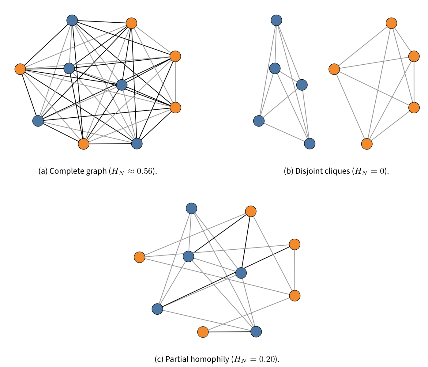
To illustrate how the network-based index behaves relative to the classic Greenberg index, consider three stylized network configurations in a population of \(n=10\) individuals, evenly divided between two language groups (\(n_A=n_B=5\), so \(p_A=p_B=\tfrac{1}{2}\) and \(H=0.5\)).
Example 1. Complete graph, equal groups. Suppose the interaction network is complete, so that every individual is connected to every other. The total number of edges is \[|E|=\binom{10}{2}=45,\] and the number of cross-language edges is \[E_{AB}=n_A n_B = 5 \times 5 = 25.\] The resulting network-based diversity index is \[H_N = \frac{E_{AB}}{|E|} = \frac{25}{45} \approx 0.56.\]
This value exceeds the population-level index \(H=0.5\) due to finite-size effects. In a complete graph, interaction pairs are formed without replacement, which slightly inflates the proportion of cross-language ties in small populations. More generally, for a complete graph the network-based index satisfies \[H_N = \frac{n}{n-1}\,H, \] so that \(H_N \to H\) as \(n \to \infty\). In large populations, the network-based and population-based indices therefore coincide (see Section ¿sec:gen_form?).
Example 2. Two disjoint cliques, equal groups. Now suppose that individuals form two separate, fully connected cliques, one consisting only of A-speakers and the other only of B-speakers. Each clique of size 5 contains \[\binom{5}{2}=10\] edges, so that the total number of edges is \[|E|=20.\] Since no edges connect individuals from different language groups, \(E_{AB}=0\) and \[H_N=\frac{0}{20}=0.\] Population composition remains unchanged, so \(H=0.5\). This example shows that effective contact diversity can be zero under complete segregation, even when population-level diversity is moderate.
Example 3. Partial homophily with a given edge split. Finally, suppose that the network contains \(|E|=20\) edges in total, of which only 20% are cross-language, corresponding to a low degree of heterophily. Then \[E_{AB}=0.2 \times 20=4 \quad \leftrightarrow \quad H_N=\frac{4}{20}=0.2.\] At the population level, \(H=0.5\), so the gap \[H-H_N=0.5-0.2=0.3\] quantifies the deficit of cross-group contact relative to the random-mixing benchmark implied by population shares.
Under a two-group stochastic block model (SBM),2 where within-group edges appear with probability \(a\) and cross-group edges with probability \(b\), the expected value of the network-based index is \[\mathbb{E}[H_N]=\frac{b\, n_A n_B}{a\binom{n_A}{2}+a\binom{n_B}{2}+b\, n_A n_B}.\] With \(n_A=n_B=5\), \(a=0.8\) and \(b=0.2\), this expression yields \(\mathbb{E}[H_N]\approx 0.238\), close to the value implied by the assumed edge split.3
The three examples are summarized in Figure 1. They illustrate how identical population-level diversity can correspond to markedly different levels of contact diversity, depending exclusively on network structure.
General formula
The illustrative cases above can be generalized by considering the benchmark case of a complete graph. Let the population consist of \(n\) individuals partitioned into \(L\) language groups, with \(n_\ell\) denoting the size of group \(\ell\) and \(n=\sum_{\ell=1}^{L} n_\ell\) the total population.
In a complete graph, the total number of edges is
| \[|E|=\binom{n}{2}=\frac{n(n-1)}{2}.\] | \[(15)\] |
| \[E_{\text{cross}}=\sum_{\ell<\ell'} n_\ell n_{\ell'}=\frac{n^2-\sum_{\ell} n_\ell^2}{2},\] | \[(16)\] |
| \[H_N = \frac{E_{\text{cross}}}{|E|} = \frac{n^2-\sum_{\ell} n_\ell^2}{n(n-1)}. \] | \[(17)\] |
By comparison, the population-level Greenberg index can be written as
| \[H = 1 - \sum_{\ell} \left(\frac{n_\ell}{n}\right)^2 = \frac{n^2-\sum_{\ell} n_\ell^2}{n^2}.\] | \[(18)\] |
| \[H_N = \frac{n}{n-1}\,H. \] | \[(19)\] |
This relationship shows that, in a complete graph, the network-based index differs from the population index only by a finite-size correction factor. As population size increases, this correction vanishes and \(H_N\) converges to \(H\). The finite-size correction arises because the Greenberg index is defined in terms of independent sampling with replacement from the population, whereas \(H_N\) is computed over a fixed set of unordered pairs formed without replacement. For large populations, this distinction becomes negligible, and the two measures coincide.
Competence-conditioned extension
The baseline formulation of the N-GDI treats linguistic difference as categorical, assigning each individual to a single language group. In many multilingual settings, however, individuals possess competences in multiple languages, and the effective linguistic distance between interlocutors depends not only on group membership but also on the overlap of their linguistic repertoires. To account for this dimension, the network-based index can be extended by replacing the binary linguistic difference with a competence-weighted measure of communicative distance.
Let \(c_{\ell u} \in [0,1]\) denote the competence in language \(\ell\) of individual \(u\), where \(c_{\ell u}=1\) indicates full mastery and \(c_{\ell u}=0\) indicates no knowledge. For each pair of individuals \((u,v)\) connected by an edge, define their communicative similarity as
| \[\text{sim}(u,v) = \max_{\ell \in \{1,\dots,L\}} \min\{c_{\ell u}, c_{\ell v}\}. \] | \[(20)\] |
The competence-conditioned N-GDI is then defined as
| \[H_N^{*} = 1 - \frac{1}{|E|} \sum_{(u,v)\in E} \text{sim}(u,v). \] | \[(21)\] |
While the binary index \(H_N\) treats all cross-language ties as equally distant, \(H_N^{*}\) discounts the contribution of an interaction whenever interlocutors share linguistic resources that enable communication.
It is important to clarify the interpretation of \(H_N^{*}\). The index does not measure whether interactions are cross-linguistic in a categorical sense. Two individuals belonging to different language groups may still interact using a shared second language, and such an interaction remains cross-linguistic from a demographic perspective. Instead, \(H_N^{*}\) measures the effective communicative distance along interaction edges. When individuals share linguistic competences that allow communication, the communicative distance between them is reduced, even though the interaction still occurs across linguistic groups.
Accordingly, \(H_N\) and \(H_N^{*}\) capture two distinct dimensions of multilingual interaction. The binary index \(H_N\) measures the extent of cross-group contact, while the competence-conditioned index \(H_N^{*}\) measures how linguistically distant those contacts are. Increasing multilingual competences therefore does not reduce cross-linguistic interaction, but reduces communicative distance within cross-linguistic interaction.
This formulation is closely related to, but distinct from, the co-competence extension of the Greenberg index discussed in Civico (2026). While the latter aggregates individual competences across the entire population, the present extension operates at the level of interactions, conditioning the contribution of each edge on the communicative overlap between its endpoints.
Example 4. Consider two individuals connected by an edge. Individual \(u\) is a native speaker of language A with partial competence in B (\(c_{Au}=1\), \(c_{Bu}=0.5\)), while individual \(v\) is a native speaker of B with no knowledge of A (\(c_{Av}=0\), \(c_{Bv}=1\)). Their communicative similarity is \[\text{sim}(u,v) = \max\{\min(1,0.5), \min(0,1)\} = 0.5.\] The edge contributes only partially to contact diversity, reflecting the fact that communication is possible, albeit imperfectly. If individual \(u\)’s competence in B were zero, the similarity between \(u\) and \(v\) would be zero and the edge would be fully counted as cross-linguistic.
By construction, \(H_N^{*}\) allows one to examine how bilingualism, second-language acquisition, or proficiency in a lingua franca alter experienced contact diversity without modifying the underlying structure of social interaction.
Multi-layer networks
In many settings, social interaction is distributed across multiple domains, such as family, workplace, school, or online communication. Each domain may exhibit distinct patterns of linguistic mixing. To account for this heterogeneity, the N-GDI can be extended to a multi-layer framework, in which each layer represents a distinct interaction context.
Let \(K\) denote the number of interaction layers. Each layer \(k \in \{1,\dots,K\}\) is represented by an undirected graph with edge set \(E^{(k)}\), defined over the same set of individuals. Let \(\alpha_k \ge 0\) denote the relative weight of layer \(k\), with \(\sum_{k=1}^{K} \alpha_k = 1\). The weights reflect the relative importance or frequency of interactions in each domain.
The multi-layer Network-based Greenberg Diversity Index is defined as
| \[H_{N}^{\text{multi}} = 1 - \sum_{k=1}^{K} \alpha_k \left( \frac{1}{|E^{(k)}|} \sum_{(u,v)\in E^{(k)}} \text{sim}(u,v) \right), \] | \[(23)\] |
The multi-layer formulation does not introduce a new notion of network structure. Rather, it aggregates contact diversity across domains while preserving the probabilistic interpretation of the index. Importantly, this definition differs from computing \(H_N\) on the union of all edges across layers, i.e. as the conflation of language use patterns occurring across all layers. By averaging layer-specific contributions, it allows domains with different interaction frequencies or social relevance to affect overall contact diversity in proportion to their assigned weights.
Example 5. Two-layer network (family and workplace). Consider a population divided into two equally sized language groups. In the family layer, all edges are within-group, so \(H_N^{\text{family}}=0\). In the workplace layer, suppose that half of the ties are cross-language, so \(H_N^{\text{work}}=0.5\). If family and workplace interactions are equally weighted (\(\alpha_{\text{family}}=\alpha_{\text{work}}=0.5\)), then \[H_N^{\text{multi}} = 0.5 \times 0 + 0.5 \times 0.5 = 0.25.\] The aggregate contact diversity lies between the two layer-specific values, reflecting the combined influence of the two domains.
Example 6. Adding an online layer. Suppose a third layer captures online interactions, where linguistic mixing is frequent and \(H_N^{\text{online}}=0.7\). If the weights are \(\alpha_{\text{family}}=0.2\), \(\alpha_{\text{work}}=0.5\), and \(\alpha_{\text{online}}=0.3\), then \[H_N^{\text{multi}} = 0.2 \times 0 + 0.5 \times 0.5 + 0.3 \times 0.7 = 0.46.\] Compared with the two-layer case, the inclusion of online interactions increases overall contact diversity, even though family interactions remain fully homogeneous.
Objective and subjective diversity
The N-GDI makes it possible to distinguish formally between objective and subjective diversity, following the conceptual distinction proposed by Grin (2003). Objective diversity refers to the stock and distribution of languages within a population, as captured by population-based indices such as \(H\). Subjective diversity refers to the diversity individuals are exposed to through their actual social interactions.
Because subjective diversity depends on contact structure, the two dimensions need not move in the same direction. Changes in mobility, institutional organization, or communication practices may alter interaction patterns without modifying population composition. Conversely, demographic change may affect objective diversity without substantially altering everyday contact.
The N-GDI captures this distinction directly. For a fixed population composition, \(H_N\) decreases under segregation and increases as interaction across language groups intensifies. As a result, subjective diversity may increase even when objective diversity declines, or vice versa.
Example 7. Consider two periods. At time \(t_0\), there are three equally sized language groups that are fully segregated into disjoint cliques. Objective diversity is relatively high, with \[H = 1 - 3\cdot\left(\tfrac{1}{3}\right)^2 = \tfrac{2}{3},\] but since all interactions occur within groups, \(H_N=0\), indicating that individuals experience no subjective diversity through direct interaction, even though diversity is still present in the broader social environment.
At time \(t_1\), assume that homogenizing forces have led to the survival of only two language groups of equal size. In this case, objective diversity decreases to: \[H = 1 - 2\cdot\left(\tfrac{1}{2}\right)^2 = \tfrac{1}{2}.\] If interaction is now well mixed across the two groups, the network-based index satisfies \(H_N \approx 0.5\). Between \(t_0\) and \(t_1\), objective diversity decreased, while subjective diversity increased. This example illustrates how demographic composition and contact structure may evolve in different directions.
Taken together, these definitions establish the Network-based Greenberg Diversity Index as a tool for distinguishing between diversity embedded in population composition and diversity experienced through social interaction.
Model
To examine how contact diversity responds to different patterns of social interaction, we analyze a set of stylized contact network archetypes. These archetypes serve as controlled constructions designed to isolate the effect of network structure on the Network-based Greenberg Diversity Index.
Across all scenarios, total population is held fixed (though group proportions are allowed to change), while interaction patterns vary systematically. For each configuration, we compute the population-based Greenberg index \(H\), the network-based index \(H_N\), and their difference \(\Delta = H - H_N\). This design allows us to distinguish the role of demographic composition from that of contact structure, and to assess how departures from random mixing affect realized diversity.
We focus on four baseline network archetypes that differ in topology and mixing patterns: complete graphs, complete segregation, bridged segregation, and core–periphery structures. In addition, the competence-conditioned and multi-layer formulations introduced above are used to examine how linguistic repertoires and multiple interaction domains modulate contact diversity.
The competence-conditioned extension is applied as an overlay on a fixed network: node labels and edges are held constant, while language-competence vectors modify the communicative distance associated with each edge. The multi-layer extension, by contrast, represents distinct interaction domains through separate family and work layers, and then aggregates layer-specific contact diversity using predefined weights.
Complete graph
As a benchmark, we consider a complete graph in which every individual is connected to every other. Edges are formed independently of linguistic attributes, so interaction is unconstrained by group membership. This configuration corresponds to the random-mixing assumption underlying the classic Greenberg index and serves as a reference case for the network-based formulation.
In a complete graph, the network-based index \(H_N\) differs from the population-level index \(H\) only through the finite-size correction derived in Section 3. As population size increases, this correction vanishes and the two measures coincide. Any divergence between \(H_N\) and \(H\) observed in the remaining archetypes can therefore be attributed to structural constraints on contact rather than to population composition.
Complete segregation
At the opposite extreme of the benchmark case, we consider complete segregation. The population is partitioned into disjoint subgraphs, one for each language group, with no edges connecting individuals across groups. Within each group, all individuals are connected to one another, forming fully connected cliques.
In this configuration, the population-level index \(H\) remains strictly positive whenever more than one language group is present. By contrast, the network-based index satisfies \(H_N=0\), because all observed interactions occur within groups. The resulting gap \(\Delta = H - H_N\) therefore reflects the full divergence between demographic diversity and contact diversity induced by complete structural separation.
Bridged segregation
An intermediate configuration between complete segregation and random mixing is obtained by introducing a limited number of cross-group ties between otherwise segregated groups. In this archetype, individuals within each language group form a dense subgraph, while a small number of edges connect individuals belonging to different groups.
Formally, the network consists of two within-group cliques, one for each language group, augmented by a set of cross-group edges. The number of such bridging edges is treated as a free parameter. All other aspects of population composition are held constant.
In this configuration, the network-based index \(H_N\) is strictly positive but typically remains below the population-level index \(H\) when the number of cross-group ties is small. As additional bridging edges are added, the proportion of cross-group interactions increases and \(H_N\) rises monotonically, reducing the gap \(\Delta = H - H_N\). This construction allows us to trace how contact diversity responds to incremental increases in cross-group connectivity, holding within-group cohesion fixed.
Core–periphery structure
We next consider a core–periphery topology. The population is divided into two subsets: a densely connected core and a sparsely connected periphery. Core nodes form a tightly knit subgraph, while peripheral nodes have few connections and are linked mainly to the core rather than to one another.
Unlike the bridged segregation archetype, which models separation through explicit clustering by language, the core–periphery configuration is used here to introduce a positional contrast within the network. More precisely, we impose an asymmetry between central and peripheral locations by assigning language groups differently across these two structural zones. The purpose is not to assume that the core is “naturally” more diverse than the periphery, but to examine how the placement of linguistic heterogeneity within the network affects realized contact diversity.5
In this setting, any deviation of \(H_N\) from the demographic benchmark \(H\) arises not from an explicit preference for same-language ties, but from the way contacts are distributed across structurally unequal positions. Because interactions are concentrated in the core, which dominates the flow of information and contact, the location of cross-group ties matters in addition to their overall number. Peripheral nodes may therefore remain relatively isolated from linguistic diversity even when they are connected to a more heterogeneous center, simply because of asymmetries in degree and network centrality.
Extensions
The competence-conditioned and multi-layer formulations are applied to the baseline network archetypes in order to examine how contact diversity is affected by additional dimensions of heterogeneity. These extensions refine the measurement of contact diversity in two different ways. The competence-conditioned extension modifies the evaluation of edges within a given topology by conditioning linguistic distance on shared competences. The multi-layer extension represents interaction domains as distinct layers and aggregates the corresponding layer-specific indices. Together, they allow us to assess how linguistic competences and multiple interaction contexts affect the relation between population diversity and realized contact.
The competence-conditioned extension relaxes the categorical treatment of linguistic difference by allowing each interaction to contribute to contact diversity in proportion to the strength of the best shared communicative channel between the connected individuals. Network structure is held fixed, while linguistic repertoires vary across nodes. In this way, the extension isolates the effect of multilingual competences on effective contact diversity.
The multi-layer extension accounts for the fact that interactions may occur across multiple domains, each characterized by its own pattern of linguistic mixing. Contact diversity is computed separately within each layer and then aggregated using predefined weights. This formulation preserves the probabilistic interpretation of the index while allowing different domains to contribute unevenly to overall exposure.
Together, these extensions allow us to assess how linguistic competences and multiple interaction contexts affects the relation between population diversity and realized contact.
Diagnostics
In addition to the diversity indices, we record a number of standard network statistics that characterize the structure of the contact networks generated under each archetype. These diagnostics provide complementary information about connectivity patterns and are reported alongside \(H\) and \(H_N\). We focus on three measures:
- Assortativity by language, defined following Newman (2003) as
where \(e_{\ell\ell'}\) denotes the proportion of edges linking nodes of language \(\ell\) to nodes of language \(\ell'\). In an undirected network, \(a_{\ell}=b_{\ell}\). Positive values indicate an excess of within-language ties relative to random mixing, values near zero indicate mixing patterns that are approximately independent of language, and negative values indicate a relative prevalence of cross-language ties. In other words, assortativity compares the observed share of same-language ties to the share that would be expected if edges were formed independently of language composition.6\[r=\frac{\sum_{\ell} e_{\ell\ell}-\sum_{\ell} a_{\ell}b_{\ell}} {1-\sum_{\ell} a_{\ell}b_{\ell}}, \qquad a_{\ell}=\sum_{\ell'} e_{\ell\ell'}, \qquad b_{\ell}=\sum_{\ell'} e_{\ell'\ell},\] \[(28)\] - Average degree, defined as \(\bar{k} = 2|E|/n\), which summarizes the overall density of the network. This measure reflects the average number of interaction partners per individual.
- Transitivity-based clustering coefficient, defined as \(3\frac{\text{number of triangles}}{\text{number of connected triples}}\). This statistic measures the global tendency of connected triples to close into triangles and is used here as a network-level indicator of local closure.
These diagnostics are computed for all baseline archetypes. When applicable, they are also reported for competence-conditioned and multi-layer configurations, using the same underlying network structure. Together, they provide a concise description of network properties that may co-vary with contact diversity across scenarios.
Simulation protocol
For each network archetype described above, we generate contact networks, compute the corresponding diversity indices, and record the diagnostics defined in Section (???). The simulation procedure follows three steps.
- Setup. We fix the population size \(n\) and the group sizes \(\{n_\ell\}\), which determine the population-level Greenberg index \(H\). Languages are assigned to individuals according to the specified population composition. For each archetype, we also specify the parameters governing network construction, such as the number of bridging edges, the size of the core, the probabilities of edge formation, competence levels, or layer weights.
- Network generation. Some configurations yield deterministic structures, such as complete graphs or disjoint cliques, while others involve stochastic elements, such as probabilistic core–periphery ties or rewired multi-layer networks. In the latter case, each simulation run corresponds to an independent realization of the same underlying generative process.
- Measurement. For each generated network, we compute the population-based index \(H\), the network-based index \(H_N\), and their difference \(\Delta = H - H_N\). When competence-conditioned or multi-layer extensions are applied, we compute the corresponding indices \(H_N^{*}\) or \(H_N^{\text{multi}}\) as defined in Section ¿sec:definition?. We also record the diagnostic network statistics for each realization.
For stochastic archetypes, the same parameter setting is simulated repeatedly, since each run may generate a different network. Reported results therefore summarize the distribution of outcomes across replications, typically through sample means and dispersion measures. By contrast, deterministic archetypes generate a single network for each parameter setting, so the reported values correspond directly to that unique realization. Within each archetype, parameters are then varied systematically to examine how the indices respond to changes in network structure.7
Simulation Results
Tables 1, 2 and 3 provide a synthetic overview of the main archetypes.
| Archetype | \(n_{\text{bridges}}\) | \(H\) | \(H_N\) | \(\Delta\) | Assort. | \(C\) |
|---|---|---|---|---|---|---|
| Baseline archetypes | ||||||
| Complete graph | – | 0.50 | 0.508 | \(-0.008\) | \(-0.017\) | 1.000 |
| Disjoint cliques | – | 0.50 | 0.000 | 0.500 | 1.000 | 1.000 |
| Bridged segregation sweep | ||||||
| Bridged cliques | 1 | 0.50 | 0.001 | 0.499 | 0.998 | 0.998 |
| Bridged cliques | 5 | 0.50 | 0.006 | 0.494 | 0.989 | 0.988 |
| Bridged cliques | 10 | 0.50 | 0.011 | 0.489 | 0.977 | 0.977 |
| Bridged cliques | 30 | 0.50 | 0.033 | 0.467 | 0.933 | 0.936 |
| Bridged cliques | 100 | 0.50 | 0.103 | 0.397 | 0.794 | 0.831 |
Benchmarks: Complete graph and complete segregation
We begin with the two benchmark configurations. In the complete graph, where every individual is connected to every other, the network-based index \(H_N\) coincides with the population-based index \(H\) up to the finite-size correction discussed in Section 3. In our simulations with \(n=60\) and two equally sized language groups, \(H=0.5\) and \(H_N \approx 0.508\), with zero variance across replications. This confirms that the N-GDI reproduces the classic Greenberg index under random mixing.
At the opposite extreme, complete segregation yields \(H_N=0\) despite \(H=0.5\). All interactions occur within language groups, and the gap \(\Delta\) reaches its maximum value.
These two configurations provide the range of possible divergences between demographic diversity and contact diversity and serve as reference points for the bridged segregation structures discussed below.
Bridged segregation
The bridged segregation archetype introduces a controlled number of cross-group ties between otherwise segregated language communities. As expected, the network-based index \(H_N\) increases monotonically with the number of bridging edges, while the demographic index \(H\) remains constant by construction. When bridges are sparse, contact diversity remains substantially below population diversity. As additional bridges are added, \(H_N\) rises and the gap \(\Delta = H - H_N\) narrows. We plot this relationship (for a population of \(n=60\)) in Figure 2, which reports \(H_N\) as a function of the number of cross-group bridges together with the corresponding gap \(\Delta\).
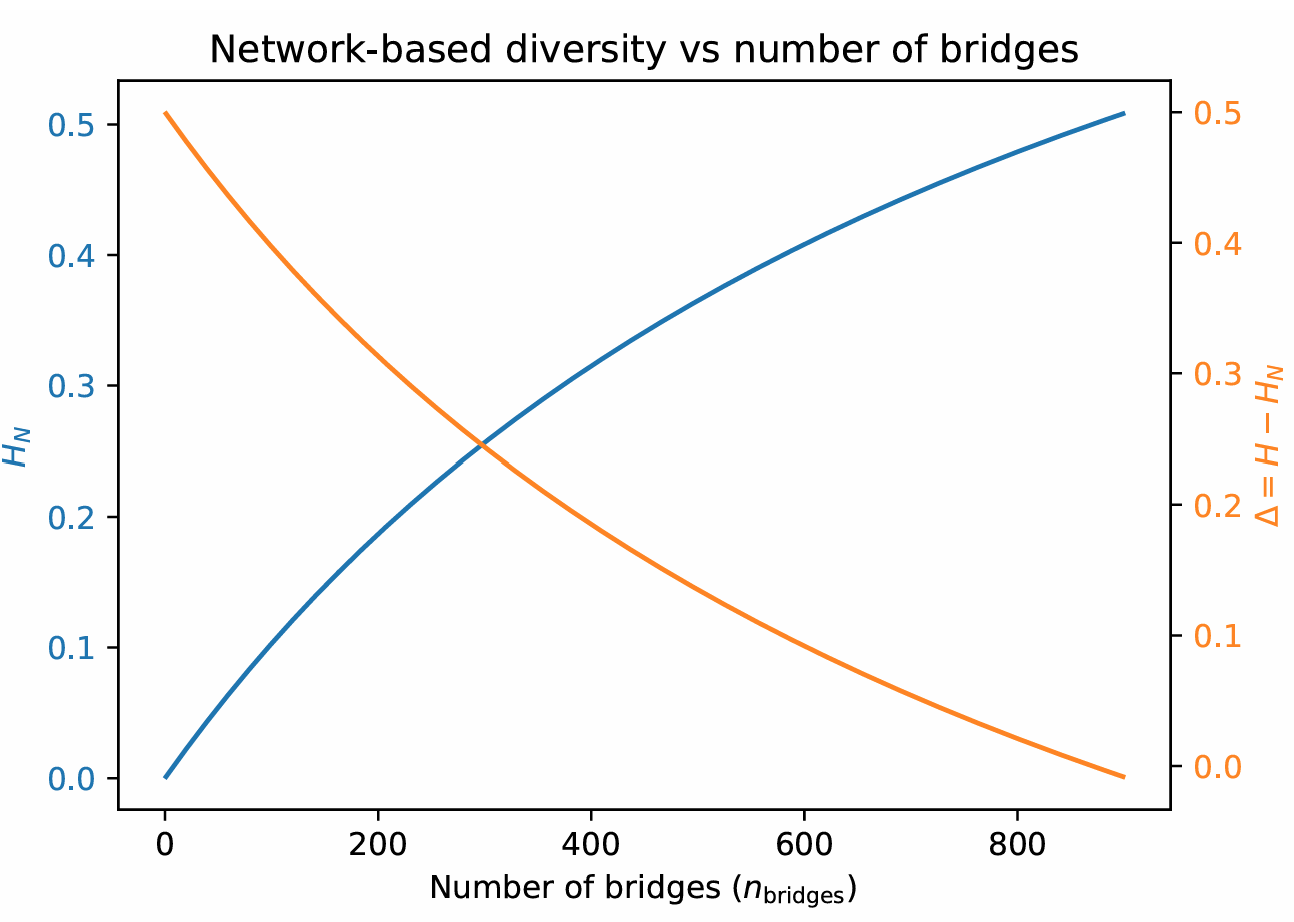
The figure shows that even very few bridging ties can generate measurable increases in contact diversity, while further additions produce progressively smaller gains. At the same time, the results highlight that demographic diversity alone is not informative about realized interaction: configurations with identical \(H\) may exhibit very different levels of \(H_N\) depending on the prevalence of cross-group connectivity.
Core–periphery
We now examine how the core–periphery structure affects contact diversity in simulated networks. Two parameters control the topology: the core fraction \(\mathit{cf} \in \{0.20, 0.30, 0.40, 0.50, 0.60\}\), which specifies the share of individuals assigned to the densely connected core, and the core–periphery connection probability \(p_{cp} \in \{0.04, 0.06, 0.10, 0.20\}\), which determines the likelihood of ties between core and peripheral nodes. The probability of internal core edges is fixed at \(p_{\text{core}} = 0.25\), and periphery–periphery edges are sparse (\(p_{\text{per}} = 0.02\)).
Language groups are assigned asymmetrically across structural positions. The core is internally mixed, with 50% of its nodes assigned to each language, while the periphery is entirely monolingual in language A. As a result, demographic diversity is not held constant across simulations. Instead, it increases mechanically with the size of the core, because a larger core contains a larger share of B-speakers. In the present setup, realized population diversity rises from \(H=0.180\) when \(\mathit{cf}=0.20\) to \(H=0.420\) when \(\mathit{cf}=0.60\).
| Archetype | \(\mathit{cf}\) | \(p_{cp}\) | \(H\) | \(H_N\) | \(\Delta\) | Assort. |
|---|---|---|---|---|---|---|
| Core–periphery | 0.20 | 0.04 | 0.180 | 0.319 | \(-0.139\) | 0.083 |
| Core–periphery | 0.20 | 0.06 | 0.180 | 0.337 | \(-0.157\) | 0.032 |
| Core–periphery | 0.20 | 0.10 | 0.180 | 0.365 | \(-0.185\) | \(-0.087\) |
| Core–periphery | 0.20 | 0.20 | 0.180 | 0.429 | \(-0.249\) | \(-0.174\) |
| Core–periphery | 0.30 | 0.04 | 0.255 | 0.413 | \(-0.158\) | 0.031 |
| Core–periphery | 0.30 | 0.06 | 0.255 | 0.427 | \(-0.172\) | \(-0.009\) |
| Core–periphery | 0.30 | 0.10 | 0.255 | 0.445 | \(-0.190\) | \(-0.082\) |
| Core–periphery | 0.30 | 0.20 | 0.255 | 0.464 | \(-0.209\) | \(-0.150\) |
| Core–periphery | 0.40 | 0.04 | 0.320 | 0.458 | \(-0.138\) | 0.024 |
| Core–periphery | 0.40 | 0.06 | 0.320 | 0.476 | \(-0.156\) | \(-0.036\) |
| Core–periphery | 0.40 | 0.10 | 0.320 | 0.478 | \(-0.158\) | \(-0.087\) |
| Core–periphery | 0.40 | 0.20 | 0.320 | 0.479 | \(-0.159\) | \(-0.137\) |
| Core–periphery | 0.50 | 0.04 | 0.375 | 0.482 | \(-0.107\) | \(-0.008\) |
| Core–periphery | 0.50 | 0.06 | 0.375 | 0.480 | \(-0.105\) | \(-0.017\) |
| Core–periphery | 0.50 | 0.10 | 0.375 | 0.496 | \(-0.121\) | \(-0.065\) |
| Core–periphery | 0.50 | 0.20 | 0.375 | 0.499 | \(-0.124\) | \(-0.126\) |
| Core–periphery | 0.60 | 0.04 | 0.420 | 0.497 | \(-0.077\) | \(-0.006\) |
| Core–periphery | 0.60 | 0.06 | 0.420 | 0.498 | \(-0.078\) | \(-0.020\) |
| Core–periphery | 0.60 | 0.10 | 0.420 | 0.513 | \(-0.093\) | \(-0.066\) |
| Core–periphery | 0.60 | 0.20 | 0.420 | 0.505 | \(-0.085\) | \(-0.089\) |
Figure 3 reports average contact diversity \(H_N\) across parameter settings together with the corresponding realized value of \(H\) for each core fraction. Several patterns emerge. First, for a given core size, increasing \(p_{cp}\) generally leads to higher \(H_N\). Indeed, greater coupling gives peripheral nodes more access to the mixed core, thereby increasing the share of cross-language ties. Second, for fixed \(p_{cp}\), increasing the size of the core also raises \(H_N\), because a larger share of the network is occupied by diverse and highly connected individuals.
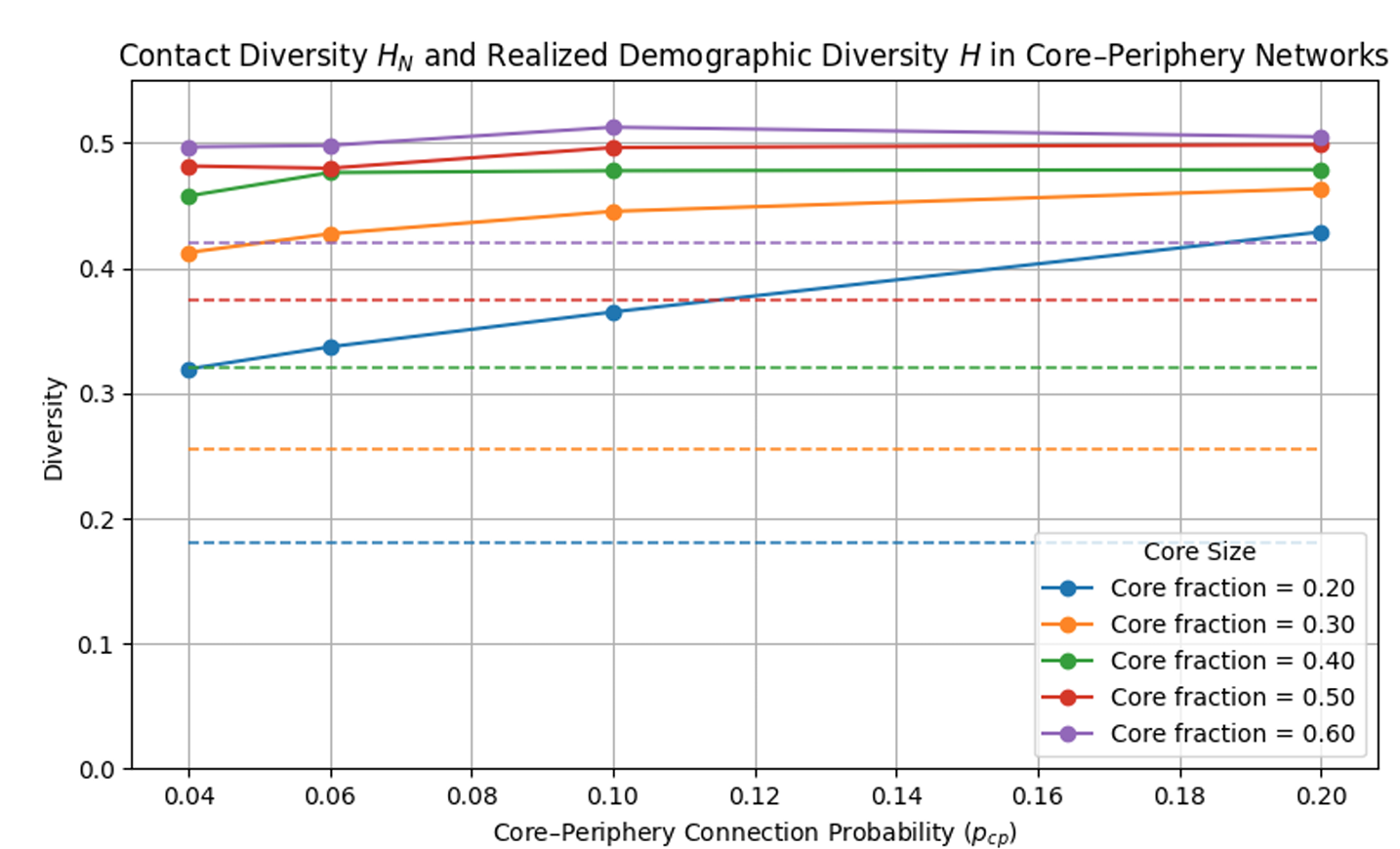
The fact that \(H_N\) exceeds \(H\) in all configurations is not surprising. The two indices sample different objects. The quantity \(H\) is computed from node shares, whereas \(H_N\) is computed from edges. In the present setup, linguistic heterogeneity is concentrated in the core, which is also the structurally dominant part of the network in terms of connectivity. As a result, B-speakers account for a larger share of interactions than of the population. Cross-language encounters are therefore overrepresented in the edge sample relative to the node sample, which pushes \(H_N\) above \(H\).
This result clarifies that contact diversity is shaped not only by the prevalence of cross-group ties but also by their structural location. In a core–periphery network, diversity concentrated in the most connected part of the graph can generate a level of contact diversity that exceeds what one would infer from population shares alone. The mechanism is therefore distinct from the bridged-segregation case. There, increases in \(H_N\) come from adding direct links between otherwise segregated groups. Here, by contrast, cross-group exposure is amplified because the mixed group occupies the central and interaction-rich portion of the network.
Competence-conditioned contact diversity
We next consider the competence-conditioned extension of the N-GDI. In this scenario, the underlying network structure and the assignment of language labels are held fixed, using a core–periphery topology with a nominally imbalanced two-group population of sizes \((20,40)\). If these group sizes were realized directly in the graph, they would imply a demographic diversity of
| \[H = 1 - \left(\frac{20}{60}\right)^2 - \left(\frac{40}{60}\right)^2 \approx 0.444.\] | \[(29)\] |
Because the language labels are fixed across the sweep, realized demographic diversity is constant across all \(L_2\) values. In the present setup, however, realized population diversity is not equal to the nominal benchmark implied by the input group sizes. Under the current core–periphery assignment rule, the core is internally mixed while the periphery is entirely assigned to language A. With a core fraction of \(0.35\) in a population of \(60\) nodes, this produces a realized distribution of \(50\) A-speakers and \(10\) B-speakers, yielding
| \[H = 1 - \left(\frac{50}{60}\right)^2 - \left(\frac{10}{60}\right)^2 \approx 0.278,\] | \[(30)\] |
| (a) Competence-conditioned contact diversity | |||||
|---|---|---|---|---|---|
| Archetype | \(L_2\) | \(H\) | \(H_N\) | \(H_N^*\) | \(\Delta\) |
| Core–periphery + competence | 0.00 | 0.278 | 0.435 | 0.435 | \(-0.157\) |
| Core–periphery + competence | 0.10 | 0.278 | 0.435 | 0.391 | \(-0.157\) |
| Core–periphery + competence | 0.20 | 0.278 | 0.435 | 0.348 | \(-0.157\) |
| Core–periphery + competence | 0.30 | 0.278 | 0.435 | 0.304 | \(-0.157\) |
| Core–periphery + competence | 0.40 | 0.278 | 0.435 | 0.261 | \(-0.157\) |
| Core–periphery + competence | 0.50 | 0.278 | 0.435 | 0.217 | \(-0.157\) |
| Core–periphery + competence | 0.60 | 0.278 | 0.435 | 0.174 | \(-0.157\) |
| Core–periphery + competence | 0.70 | 0.278 | 0.435 | 0.130 | \(-0.157\) |
| Core–periphery + competence | 0.80 | 0.278 | 0.435 | 0.087 | \(-0.157\) |
| Core–periphery + competence | 0.90 | 0.278 | 0.435 | 0.043 | \(-0.157\) |
| Core–periphery + competence | 1.00 | 0.278 | 0.435 | 0.000 | \(-0.157\) |
| (b) Multi-layer contact networks | |||||
| Archetype | \(\alpha_{\text{family}}\) | \(H\) | \(H_N\) (union) | \(H_N^{\text{multi}}\) | \(\Delta\) |
| Family–work multilayer | 0.2 | 0.50 | 0.337 | 0.401 | 0.163 |
| Family–work multilayer | 0.4 | 0.50 | 0.334 | 0.351 | 0.166 |
| Family–work multilayer | 0.6 | 0.50 | 0.331 | 0.302 | 0.169 |
| Family–work multilayer | 0.8 | 0.50 | 0.330 | 0.252 | 0.170 |
As expected, the binary network-based index \(H_N\) remains constant across all competence levels (\(H_N \approx 0.435\)), since the structure of social ties and the placement of language groups are unchanged by construction. By contrast, the competence-conditioned index \(H_N^*\) decreases smoothly from approximately \(0.435\) to \(0\) as second-language competence increases. When second-language competence is zero, \(H_N^*\) coincides exactly with \(H_N\); as competence rises, linguistic overlap across existing ties increases, reducing effective communicative distance. Under full mutual intelligibility, all interactions become linguistically transparent and \(H_N^*\) converges to zero.
This result illustrates that the competence-conditioned measure of contact diversity can collapse even in the absence of any change in network structure. In the present setup, both realized demographic diversity and contact structure remain fixed, yet experienced communicative distance declines continuously due to the expansion of shared linguistic repertoires. The distinction between \(H_N\) and \(H_N^*\) is therefore crucial: the former captures the extent of cross-group interaction, whereas the latter captures how linguistically distant those interactions remain once communicative overlap is taken into account.
It is also worth noting that, in this configuration, \(H_N\) exceeds \(H\). The quantity \(H\) is computed from node shares, whereas \(H_N\) is computed from edges. Since minority-language speakers are concentrated in the mixed and highly connected core, they account for a larger share of interactions than of the population. Cross-language ties are therefore overrepresented in the edge sample relative to the node sample, which is why \(\Delta = H - H_N\) is negative throughout.
Multi-layer contact networks
We now turn to the multi-layer extension of the N-GDI, which accounts for the fact that individuals interact across multiple social domains. We consider a two-layer configuration in which the same individuals, with the same language labels, are embedded in two distinct interaction networks. The first layer represents family or intimate ties and is characterized by strong homophily by language. The second layer represents professional or workplace ties and exhibits weaker homophily, with more frequent cross-group contact.
Both layers are generated from a common baseline network and then modified by edge rewiring in order to produce different levels of assortativity by language. In other words, the total number of ties attached to each individual is kept fixed, but some ties are redirected so that they connect different pairs of nodes. In this way, each person retains the same degree, that is, the same number of contacts, while the linguistic composition of those contacts can change. The procedure therefore isolates mixing patterns by language from overall variation in network density or individual connectedness.8
In the family layer, rewiring is used to increase assortativity, so that ties are concentrated more strongly within language groups. This produces a more segregated structure and, accordingly, a lower level of contact diversity \(H_N^{\mathrm{fam}}\). In the workplace layer, rewiring instead targets a lower assortativity level, so that a larger share of ties runs across language groups. This yields a more integrated structure and a higher level of contact diversity \(H_N^{\mathrm{work}}\). The same language assignment is used in both layers, reflecting the fact that individuals do not change group membership across domains. Operationally, one may think of the rewiring step as replacing two ties, such as \((u,v)\) and \((x,y)\), with two new ties, such as \((u,x)\) and \((v,y)\), whenever this moves the network closer to the desired level of assortativity. Because each node remains incident to the same number of ties, degrees are preserved throughout.
Contact diversity in the multi-layer setting is summarized by a weighted index
| \[H_N^{\mathrm{multi}} = \alpha_{\mathrm{family}} \, H_N^{\mathrm{fam}} + (1 - \alpha_{\mathrm{family}})\, H_N^{\mathrm{work}}\] | \[(31)\] |
Across these parameter conditions, average \(H_N^{\mathrm{multi}}\) decreases as more interaction weight is assigned to the homophilic family layer. In our parameter sweep, the multi-layer index declines from approximately \(0.40\) when \(\alpha_{\mathrm{family}} = 0.2\) to about \(0.25\) when \(\alpha_{\mathrm{family}} = 0.8\). Throughout, \(H_N^{\mathrm{multi}}\) remains well below the demographic benchmark \(H = 0.5\), indicating that even when professional ties are relatively more mixed, domain-specific homophily and limited cross-group contact in the family layer substantially reduce overall exposure.
These results underscore two distinct sources of diversity distortion. First, segregation in specific domains directly lowers contact diversity, as seen in the strongly homophilic family layer. Second, even domains that are only partially integrated, such as the workplace layer, do not fully propagate demographic diversity when homophily is non-zero. The multi-layer N-GDI captures both effects by preserving the probabilistic interpretation of exposure while allowing different spheres of interaction to contribute unequally. This flexible framework reflects the layered nature of real-world contact patterns and highlights how domain-specific homophily and the allocation of interaction across domains jointly shape experienced linguistic diversity.
Discussion
This paper proposed a network-based extension of the Greenberg Diversity Index to distinguish between demographic linguistic diversity and effective communicative exposure. By embedding linguistic attributes in explicit contact structures, the Network-based Greenberg Index and its extensions make it possible to identify how interaction patterns translate population heterogeneity into experienced diversity. The simulation results clarify several conceptual and methodological issues that are directly relevant for computational social science and for the analysis and evaluation of language policies.
Relation to existing work
The proposed index is related to, but distinct from, several existing traditions in the quantitative study of language contact and linguistic diversity. Early quantitative approaches to language comparison, such as Swadesh’s work on lexicostatistics and glottochronology, used pairwise lexical similarities to study historical relationships, diversification, and contact between languages (Swadesh 1952, 1955, 1971). The present paper adopts a different unit of analysis. It does not measure similarity between languages, but diversity across social ties connecting speakers. In this sense, the N-GDI shifts attention from linguistic relatedness to interactional exposure.
The framework also differs from agent-based and mathematical models of language competition, language change, and the emergence of contact languages. Models such as those developed by Baxter et al. (2009), Castelló et al. (2013), Tria et al. (2015), Rosillo-Rodes et al. (2023), Charalambous et al. (2023), and Buzato & Cunha (2024) typically examine how language use, linguistic variants, language ideologies, or language preferences evolve through interaction. The N-GDI has a more limited but complementary purpose. It does not model language shift or language change directly. Rather, it provides a diagnostic measure of how much linguistic diversity is realized through a given contact structure. It can therefore be used as an outcome, baseline, or descriptive statistic within dynamic models of multilingual societies.
The paper is also connected to work that treats language as a complex adaptive system and emphasizes the role of interaction in linguistic change and social cognition (Beckner et al. 2009; Hruschka et al. 2009). The N-GDI follows this general orientation by treating diversity not only as a property of populations, but also as a property of interaction systems. However, its specific contribution is measurement-oriented: it translates the probabilistic logic of the Greenberg index into network terms.
Finally, the proposed framework complements recent research on bilingualism and social networks. Studies such as Gullifer & Titone (2020), Tiv et al. (2022), Kałamała et al. (2023), Cuartero et al. (2023), and Iniesta et al. (2025) show that bilingual experience is socially structured and that language use varies across interlocutors, domains, and networks. The N-GDI is consistent with this perspective, but operates at a different level. Rather than characterizing individual bilingual experience, it provides a population-level or network-level measure of contact diversity. The competence-conditioned extension then links the two perspectives by distinguishing cross-group exposure from communicative overlap.
Diversity as an interaction-dependent property
A central result of the simulations is that linguistic diversity is not simply a property of populations, but of interaction systems. Across the baseline archetypes with fixed group shares, populations with identical demographic composition exhibit systematically different levels of contact diversity depending on how social ties are structured. The contrast between benchmark cases already makes this point: a complete graph yields \(H_N \approx H\), while disjoint cliques with the same group shares reduce contact diversity to zero. In the bridged segregation archetype, adding a handful of cross-group bridges between otherwise segregated cliques is sufficient to generate a smooth gradient of contact diversity, from almost complete isolation to partial integration, while population-level diversity remains constant.
From a modeling perspective, this reinforces the idea that diversity should be treated as an emergent property of interaction rather than as an exogenous attribute of agents. In agent-based and network-based models of multilingual societies, distributions of linguistic attributes are therefore insufficient to characterize diversity unless they are combined with explicit representations of contact. The proposed framework complements existing computational approaches to language dynamics by providing a way to quantify exposure along interaction edges rather than across populations.
The results further show that different structural mechanisms can generate different relationships between demographic and contact diversity. In the bridged segregation archetype, the key driver is the prevalence of cross-group ties: \(H_N\) increases monotonically as bridges are added and the gap \(\Delta = H - H_N\) narrows accordingly. In the core–periphery archetype, by contrast, the mechanism operates through asymmetries in both access to diversity and the structural placement of diversity. The core is internally mixed, while the periphery is monolingual and sparsely connected to the core. As the core grows and core–periphery ties become denser, \(H_N\) increases, reflecting greater exposure to cross-group interaction. At the same time, realized demographic diversity \(H\) also rises with core size, because a larger core contains a larger share of minority-language speakers under the current positional assignment rule.
This distinction is important because it shows that contact diversity need not be lower than demographic diversity. In the bridged segregation case, \(H_N < H\) because cross-group interaction is restricted by construction. In the core–periphery case, however, the mixed portion of the population is concentrated in the most connected part of the graph. Since \(H\) is computed from node shares whereas \(H_N\) is computed from edges, minority-language speakers may account for a larger share of interactions than of the population. Cross-language ties can therefore be overrepresented in the edge sample relative to the node sample, so that \(H_N > H\). The simulations thus identify at least two analytically distinct dimensions shaping contact diversity: the prevalence of cross-group ties and the concentration of interaction pathways. Bridged segregation primarily varies the former, while the core–periphery archetype varies the latter. Both dimensions affect \(H_N\), but through different structural channels.
The competence-conditioned extension highlights a second distinction, namely between structural integration and communicative overlap. Structural integration operates by reshaping who interacts with whom, as illustrated by the bridged segregation and core–periphery configurations. Communicative overlap operates by altering how interactions are experienced linguistically while holding the network structure and language labels fixed. In the competence sweep, the binary contact index \(H_N\) therefore remains constant across competence levels. By contrast, the competence-conditioned index \(H_N^*\) decreases smoothly from \(H_N\) to zero as second-language competence increases from no mutual intelligibility to full bilingualism. In this setting, realized demographic diversity and contact structure remain fixed, yet effective communicative distance collapses continuously as shared repertoires expand. This makes explicit a distinction that is often blurred in empirical and policy discussions, where bi/multilingualism and social mixing are implicitly treated as interchangeable.
The competence-conditioned results also clarify how diversity indices should be interpreted. A decline in \(H_N^*\) does not signal increased segregation or reduced integration. Rather, it reflects communicative convergence: interactions become less linguistically differentiated because shared resources increase. Linguistic diversity, communicative distance, and communicative barriers are therefore analytically distinct dimensions that need not move in the same direction. By conditioning diversity on competence at the level of interactions, the proposed index avoids conflating heterogeneity with lack of mutual intelligibility. This distinction is particularly relevant for multilingual societies in which stable group identities coexist with widespread bilingualism. In such settings, population-level diversity may remain high while communicative barriers are low, or vice versa.
The multi-layer extension adds a further refinement by showing how domain-specific homophily and the allocation of interaction across domains jointly shape exposure. In the two-layer family–work configuration, the same individuals appear in both layers with identical language labels, but edges are rewired to produce stronger homophily in the family domain and weaker homophily in the professional domain. The resulting layer-specific indices satisfy \(H_N^{\mathrm{fam}} < H_N^{\mathrm{work}} < H\), and the multi-layer index \(H_N^{\mathrm{multi}}\) decreases monotonically as more interaction weight is assigned to the family layer. In the simulations, \(H_N^{\mathrm{multi}}\) falls from about \(0.40\) to \(0.25\) as the share of family-based interaction increases from \(20\%\) to \(80\%\), while \(H\) remains fixed at \(0.5\). This demonstrates that even when a more integrated domain exists, strongly homophilic interactions in another domain can substantially depress overall contact diversity if they occupy a large share of everyday interaction.
Taken together, these results show that demographic diversity, structural exposure, and communicative overlap are separable components of linguistic diversity. Population composition remains a useful reference point, but network structure and domain-specific homophily determine how much of that potential is realized, and communicative competences determine how differentiated interactions remain once contact occurs. The N-GDI and its extensions provide a set of coordinated indices that make these distinctions explicit and quantifiable.
Implications for language policy and policy evaluation
Although the contribution is primarily methodological, the results have direct implications for language policy analysis and evaluation. First, policies that target population composition, formal language status, or symbolic recognition alone are unlikely to affect communicative exposure unless they also reshape interaction structures. The disjoint cliques and bridged segregation results illustrate how strong structural separation across schools, neighborhoods, institutions, or social domains can reduce contact diversity to near zero even in demographically diverse societies, and how modest increases in intergroup connectivity can yield non-linear gains in exposure.
Second, the core–periphery simulations highlight the relevance of access to diverse centers. Settings in which a mixed and highly connected core coexists with a large monolingual periphery are compatible with substantial cross-group contact at the center, but with very unequal exposure across structural positions. Policies that concentrate diversity in a few central institutions or neighborhoods, without ensuring broad access to those spaces, may therefore produce less evenly distributed exposure than aggregate indicators suggest. Conversely, policies that expand access to diverse cores, for instance through transport, schooling, or institutional design, can increase contact diversity even without changes in nominal population composition. At the same time, the simulations also show that when diversity is concentrated in highly connected locations, cross-group contact may be overrepresented in interaction terms relative to population shares alone.
Third, policies that promote structural integration and policies that promote language learning operate on different levels. Structural interventions affect who interacts with whom, while competence-oriented interventions affect how distant those interactions are linguistically. The simulations suggest that these two levers are not functionally equivalent. Increasing bilingual competence does not create contact where none exists, and increasing contact does not by itself remove communicative distance in the absence of shared linguistic resources. The competence-conditioned results show that high levels of bilingualism can substantially reduce communicative distance without altering network structure, whereas changes in structure can raise or lower exposure independently of competence.
Fourth, the distinction between \(H_N\) and \(H_N^*\) offers a diagnostic tool for policy evaluation. Low values of \(H_N\) point to structural barriers limiting interaction across groups. Large gaps between \(H_N\) and \(H_N^*\) indicate unrealized communicative potential within existing networks: individuals have the competences needed to communicate across groups, but interaction opportunities remain limited or segregated. This distinction can help identify whether limited exposure arises primarily from lack of contact or from lack of shared competences, and thus guide the choice and sequencing of policy instruments.
The multi-layer analysis further suggests that policy interventions should be domain-sensitive. Family, neighborhood, workplace, education, and civic participation may exhibit different levels of homophily and different weights in everyday contact. Policies that act on only one domain may therefore have limited effects on overall exposure if other domains remain highly segregated and occupy a large share of interaction. The multi-layer N-GDI provides a way to formalize this intuition by weighting domain-specific indices according to their relative importance in individuals’ interactions.
Limitations and directions for future research
The proposed framework is intentionally stylized and subject to several limitations that point to promising directions for future work. First, the simulation analysis relies on synthetic network archetypes rather than empirical interaction data. The complete graph, disjoint cliques, bridged cliques, core–periphery structures, and multi-layer family–work networks are deliberately simplified representations designed to isolate particular mechanisms. Applying the N-GDI to empirical contact data, for instance from surveys, administrative records, or digital trace data, is a necessary next step to assess its descriptive and explanatory power in applied settings.
Second, the simulations treat language attributes and network structure as exogenous and static. In many real contexts, however, interaction patterns and linguistic competences co-evolve over time. Contact across groups may foster language learning, while increased competence may in turn reshape interaction opportunities and institutional arrangements. Extending the framework to dynamic models in which networks and competences jointly evolve would allow the N-GDI and its extensions to be used not only as descriptive measures, but also as outcome variables in models of language change, integration, and policy intervention.
Third, the present analysis focuses on categorical languages and on a specific competence-based similarity function that captures the strongest shared communicative channel between interlocutors. While this choice is well suited to illustrate the distinction between structural exposure and communicative overlap, alternative formulations are possible. Future research could explore different similarity functions, asymmetric communication costs, task- or domain-specific language requirements, or measures of linguistic distance, depending on the context under study. Another possible extension concerns relations of symbolic domination between languages. Even where speakers share a language that could facilitate communication, that language may be marginalized, stigmatized, or excluded from legitimate public use. In such cases, communicative distance is shaped not only by competences and network structure, but also by unequal linguistic legitimacy.
Finally, the core–periphery and multi-layer configurations are themselves stylized. The assumption of a mixed core and monolingual periphery captures one possible type of center–periphery asymmetry, but does not exhaust the range of empirically relevant structures. Likewise, the two-layer family–work model abstracts from differences in tie strength, temporal dynamics, and institutional constraints across domains. Incorporating weighted ties, role-specific interactions, richer multi-layer architectures, or alternative rules linking demographic composition to structural position would further enrich the interpretation of contact diversity and broaden the applicability of the index to policy-relevant settings.
Conclusions
This paper introduced a network-based approach to linguistic diversity that shifts the analytical focus from population composition to realized patterns of interaction. By extending the Greenberg Diversity Index to contact networks, and by conditioning it on linguistic competences and interaction domains, the framework highlights three analytically distinct dimensions: demographic diversity, structural exposure, and communicative overlap. Consistent with the diagnostic perspective outlined in the introduction, the simulations are not intended as empirical models of specific societies, but as controlled exercises that isolate the mechanisms through which interaction structures shape experienced diversity.
The simulation results show that contact diversity may diverge substantially from demographic diversity, and that this divergence depends on how social ties are organized. In the benchmark and bridged-segregation cases, populations with identical demographic composition exhibit markedly different levels of contact diversity depending on network structure. In the core–periphery configuration, the results further show that not only the prevalence of cross-group ties but also their structural location matters: when linguistic heterogeneity is concentrated in the highly connected core of the network, contact diversity can exceed the level suggested by node-based population shares alone. The competence-conditioned extension shows that multilingual competences can transform communicative exposure without altering social mixing, and the multi-layer extension shows that domain-specific homophily and the allocation of interaction across domains can further modulate realized diversity.
Taken together, these findings stress the importance of treating linguistic diversity as a relational and interaction-dependent phenomenon rather than as a purely compositional one. Population composition remains an important reference point, but it is insufficient on its own to characterize the diversity individuals actually experience through contact. Network structure determines how much of potential diversity is converted into exposure, and communicative competences determine how differentiated those interactions remain once they occur.
From a methodological perspective, the proposed indices are simple, interpretable, and compatible with standard tools in computational social science. They can be applied to stylized models, empirical networks, or hybrid settings combining survey, administrative, and digital trace data. They provide a structured way to analyze how institutions, policies, and social environments shape multilingual interaction, and to diagnose whether limited exposure is driven by population composition, structural separation, or lack of shared competences.
More broadly, the framework contributes to ongoing efforts to integrate sociolinguistics, the economics of language, and computational modeling. By making explicit the mechanisms linking diversity, interaction, and communication, it offers a common analytical language for studying multilingual societies as complex systems and for evaluating the effects of language policies beyond population-level indicators.
Acknowledgements
This work was supported by the Swiss National Science Foundation under Grant 226064 (Project GLAD). The author wishes to thank Prof. François Grin and Dr. Salim Hirèche (University of Geneva) for their insightful comments and suggestions on earlier versions of this work. The author is also grateful to the two anonymous reviewers for their constructive feedback, which helped improve the clarity and precision of the manuscript.Appendix A: Large-Population Approximation for \(H_N\) Under a Two-Group SBM
Consider a population divided into two groups of size \(n_A\) and \(n_B\) (\(n=n_A+n_B\)). In a stochastic block model, each potential edge is drawn independently, with probability \(a\) if both endpoints are in the same group, and probability \(b\) if the endpoints belong to different groups. We show that \(H_N\) converges in probability to
| \[\mathbb{E}[H_N] = \frac{b\, n_A n_B}{a \binom{n_A}{2} + a \binom{n_B}{2} + b\, n_A n_B}. \] | \[(32)\] |
Step 1: Expected number of cross-group edges.
There are \(n_A n_B\) potential cross-group edges. Each appears with probability \(b\). Therefore
| \[\mathbb{E}[E_{\text{cross}}] = b \, n_A n_B.\] | \[(33)\] |
Step 2: Expected total number of edges.
Within group \(A\), there are \(\binom{n_A}{2}\) potential edges, each appearing with probability \(a\), so the expected number of within-\(A\) edges is \(a \binom{n_A}{2}\). Similarly, for group \(B\) we have \(a \binom{n_B}{2}\). Adding the expected cross-group edges yields
| \[\mathbb{E}[|E|] = a \binom{n_A}{2} + a \binom{n_B}{2} + b \, n_A n_B.\] | \[(34)\] |
Step 3: Expected contact diversity.
By definition,
| \[H_N = \frac{E_{\text{cross}}}{|E|}.\] | \[(35)\] |
Taking expectations and invoking the law of large numbers, the ratio \(E_{\text{cross}}/|E|\) converges in probability to the ratio of expectations as \(n\) grows. Hence,
| \[\mathbb{E}[H_N] \;\approx\; \frac{\mathbb{E}[E_{\text{cross}}]}{\mathbb{E}[|E|]} = \frac{b \, n_A n_B}{a \binom{n_A}{2} + a \binom{n_B}{2} + b \, n_A n_B}.\] | \[(36)\] |
This proves Equation 32.
Corollary 1. When \(a=b\) (no homophily, random mixing), the formula reduces to \[\mathbb{E}[H_N] = \frac{n_A n_B}{\binom{n}{2}} = \frac{n}{n-1}\,H,\] which coincides with the complete-graph formula in the main text. In the limit \(n \to \infty\), \(\mathbb{E}[H_N]\to H\).
Proof. Start from Equation 32. Under random mixing we have \(a=b=p\in(0,1)\), hence
| \[\mathbb{E}[H_N] = \frac{p\, n_A n_B}{p \binom{n_A}{2} + p \binom{n_B}{2} + p\, n_A n_B} = \frac{n_A n_B}{\binom{n_A}{2} + \binom{n_B}{2} + n_A n_B}.\] | \[(38)\] |
Use the binomial identity to simplify the denominator:
| \[\binom{n_A}{2} + \binom{n_B}{2} + n_A n_B = \frac{n_A(n_A-1)}{2} + \frac{n_B(n_B-1)}{2} + n_A n_B = \frac{(n_A+n_B)\big((n_A+n_B)-1\big)}{2} = \binom{n}{2},\] | \[(39)\] |
so
| \[\mathbb{E}[H_N] = \frac{n_A n_B}{\binom{n}{2}}.\] | \[(40)\] |
Next, write the classic Greenberg index for two groups as
| \[H \;=\; 1 - \left(\tfrac{n_A}{n}\right)^2 - \left(\tfrac{n_B}{n}\right)^2 = \frac{n^2 - n_A^2 - n_B^2}{n^2} = \frac{(n_A + n_B)^2 - n_A^2 - n_B^2}{n^2} = \frac{2\,n_A n_B}{n^2}.\] | \[(41)\] |
Therefore,
| \[\frac{n}{n-1}\, H = \frac{n}{n-1}\cdot \frac{2\, n_A n_B}{n^2} = \frac{2\,n_A n_B}{n(n-1)} = \frac{n_A n_B}{\binom{n}{2}} = \mathbb{E}[H_N].\] | \[(42)\] |
Finally, since \(\frac{n}{n-1}\to 1\) as \(n\to\infty\), we obtain \(\mathbb{E}[H_N]\to H\) in the large-population limit. ◻
Appendix B: Counting Cross-Language Edges in a Complete Graph
Proposition 1. Let a population be partitioned into \(L\) groups with sizes \(\{n_\ell\}_{\ell=1}^{L}\) and total size \(n=\sum_{\ell} n_\ell\). In a complete graph on \(n\) nodes, the number of edges whose endpoints belong to different groups is \[E_{\text{cross}}=\sum_{\ell<\ell'} n_\ell n_{\ell'}=\frac{n^2-\sum_{\ell} n_\ell^2}{2}.\]
Proof.. The total number of unordered pairs of individuals in a population of size \(n\) is
| \[\binom{n}{2} \;=\; \frac{n(n-1)}{2}.\] | \[(44)\] |
For each group \(\ell\) of size \(n_\ell\), the number of within-group pairs is
| \[\binom{n_\ell}{2} \;=\; \frac{n_\ell(n_\ell-1)}{2}.\] | \[(45)\] |
Summing across all groups gives the total number of within-group pairs:
| \[\sum_{\ell=1}^{L} \binom{n_\ell}{2} \;=\; \sum_{\ell=1}^{L} \frac{n_\ell(n_\ell-1)}{2}.\] | \[(46)\] |
Therefore, the number of cross-language pairs is obtained by subtracting within-group pairs from the total:
| \[E_{\text{cross}} \;=\; \binom{n}{2} - \sum_{\ell=1}^{L} \binom{n_\ell}{2}.\] | \[(47)\] |
Substituting the explicit formulas for the binomial coefficients yields
| \[E_{\text{cross}} = \frac{n(n-1)}{2} - \sum_{\ell=1}^{L} \frac{n_\ell(n_\ell-1)}{2}.\] | \[(48)\] |
Expanding terms in the sum gives
| \[E_{\text{cross}} = \frac{n(n-1)}{2} - \frac{1}{2}\sum_{\ell=1}^{L} (n_\ell^2 - n_\ell).\] | \[(49)\] |
Since \(\sum_{\ell=1}^{L} n_\ell = n\), this simplifies to
| \[E_{\text{cross}} = \frac{n(n-1)}{2} + \frac{1}{2}\left(n-\sum_{\ell=1}^{L} n_\ell^2\right).\] | \[(50)\] |
Rearranging terms leads to
| \[E_{\text{cross}} = \frac{n^2 - n}{2} + \frac{n-\sum_{\ell=1}^{L} n_\ell^2}{2} = \frac{n^2 - \sum_{\ell=1}^{L} n_\ell^2}{2}.\] | \[(51)\] |
This proves the claim.
Appendix C: Model Documentation
This appendix documents the implementation of the simulations reported in the paper. The model is implemented in Python as a single executable script that defines the diversity indices, network diagnostics, network generators, competence and multilayer extensions, simulation loops, output routines, and selected plotting routines. The complete code and the associated replication materials are publicly available in the CoMSES Net repository.
Software environment
The simulations were implemented in Python 3. The main packages used are numpy for numerical computation, pandas for tabular data handling, networkx for graph construction and network diagnostics, and matplotlib for visualization. The script creates an output directory containing replication-level and scenario-level results in .csv format, together with selected figures in image format.
Core functions
The implementation contains three main groups of functions. First, index functions compute the population-based Greenberg Diversity Index, the binary Network-based Greenberg Diversity Index, and the competence-conditioned version of the index. In all reported simulations, demographic diversity \(H\) is computed from the language labels actually realized in the generated graph rather than directly from the nominal input group sizes.
Second, diagnostic functions compute categorical assortativity by language, average degree, and graph transitivity. These diagnostics characterize the structure of the simulated networks and help interpret differences between demographic diversity and contact diversity.
Third, network-construction functions generate the stylized structures used in the simulations. These include complete graphs, disjoint language-group cliques, bridged cliques, and stochastic core–periphery networks. The multilayer simulations additionally use a common Erdős–Rényi baseline graph and degree-preserving rewiring to construct family and work layers with different levels of linguistic assortativity. Language competences are introduced as an overlay on an existing network rather than through a separate network generator.
Simulation design and parameters
All simulations contain \(n=60\) nodes. The complete-graph, disjoint-clique, bridged-clique, core–periphery, and multilayer experiments use the nominal input vector
| \[(n_A,n_B)=(30,30).\] | \[(52)\] |
The competence-conditioned experiments use the nominal input vector
| \[(n_A,n_B)=(20,40).\] | \[(53)\] |
In the core–periphery and competence-conditioned experiments, language labels are assigned according to structural position. The core is linguistically mixed, while the periphery is assigned entirely to language A. Consequently, the realized linguistic composition may differ from the nominal input vector, and \(H\) is calculated from the realized node labels.
For each generated network, the script computes demographic diversity \(H\), binary contact diversity \(H_N\), the difference
| \[\Delta = H-H_N,\] | \[(54)\] |
assortativity by language, average degree, and transitivity. Where applicable, it also computes the competence-conditioned index \(H_N^*\) or the multilayer index \(H_N^{\mathrm{multi}}\).
Each stochastic parameter configuration is simulated using \(R=10\) replications. The script sets a global seed of 7 and uses deterministic experiment-level seeds. For most experiments, the seed is a function of the experiment index and replication number. In the competence-conditioned sweep, the seed depends only on the replication number, so that the same network and language assignment are retained across all values of second-language competence within a replication.
The principal parameter settings are as follows:
Complete graph: all possible edges between the 60 nodes are present.
Disjoint cliques: all within-group edges are present and no cross-group edges are present.
Bridged cliques: two cliques of 30 nodes are connected by \(1\), \(5\), \(10\), \(30\), or \(100\) distinct cross-group edges sampled without replacement.
Core–periphery sweep: the core fraction takes the values
\[0.20,\ 0.30,\ 0.40,\ 0.50,\ 0.60,\] \[(55)\] and the core–periphery connection probability takes the values
\[0.04,\ 0.06,\ 0.10,\ 0.20.\] \[(56)\] The within-core and within-periphery connection probabilities are fixed at \(p_{\mathrm{core}}=0.25\) and \(p_{\mathrm{per}}=0.02\), respectively. The core is assigned equal proportions of languages A and B, subject to integer rounding, while the periphery is assigned entirely to language A.
Competence-conditioned sweep: a core–periphery graph is generated using a core fraction of \(0.35\), \(p_{\mathrm{core}}=0.25\), \(p_{\mathrm{cp}}=0.06\), and \(p_{\mathrm{per}}=0.02\). Minority second-language competence varies from \(0\) to \(1\) in increments of \(0.1\). Within each replication, the network and node labels are held fixed across competence levels.
Multilayer extension: family and work layers are constructed from copies of a common Erdős–Rényi baseline graph with edge probability \(0.05\). Degree-preserving rewiring is used to approach target language-assortativity values of \(0.6\) for the family layer and \(0.1\) for the work layer. The family-layer weight takes the values
\[0.2,\ 0.4,\ 0.6,\ 0.8,\] \[(57)\] while the work-layer weight is \(1-\alpha_{\mathrm{family}}\). The rewiring procedure uses at most \(50{,}000\) iterations and a stopping tolerance of \(0.01\). The realized assortativity may differ slightly from the target.
Simulation algorithm
Algorithm 1 summarizes the simulation procedure implemented in the replication script. The experiment registry specifies the network generator, nominal group sizes, parameter values, and any competence or multilayer extension associated with each scenario.
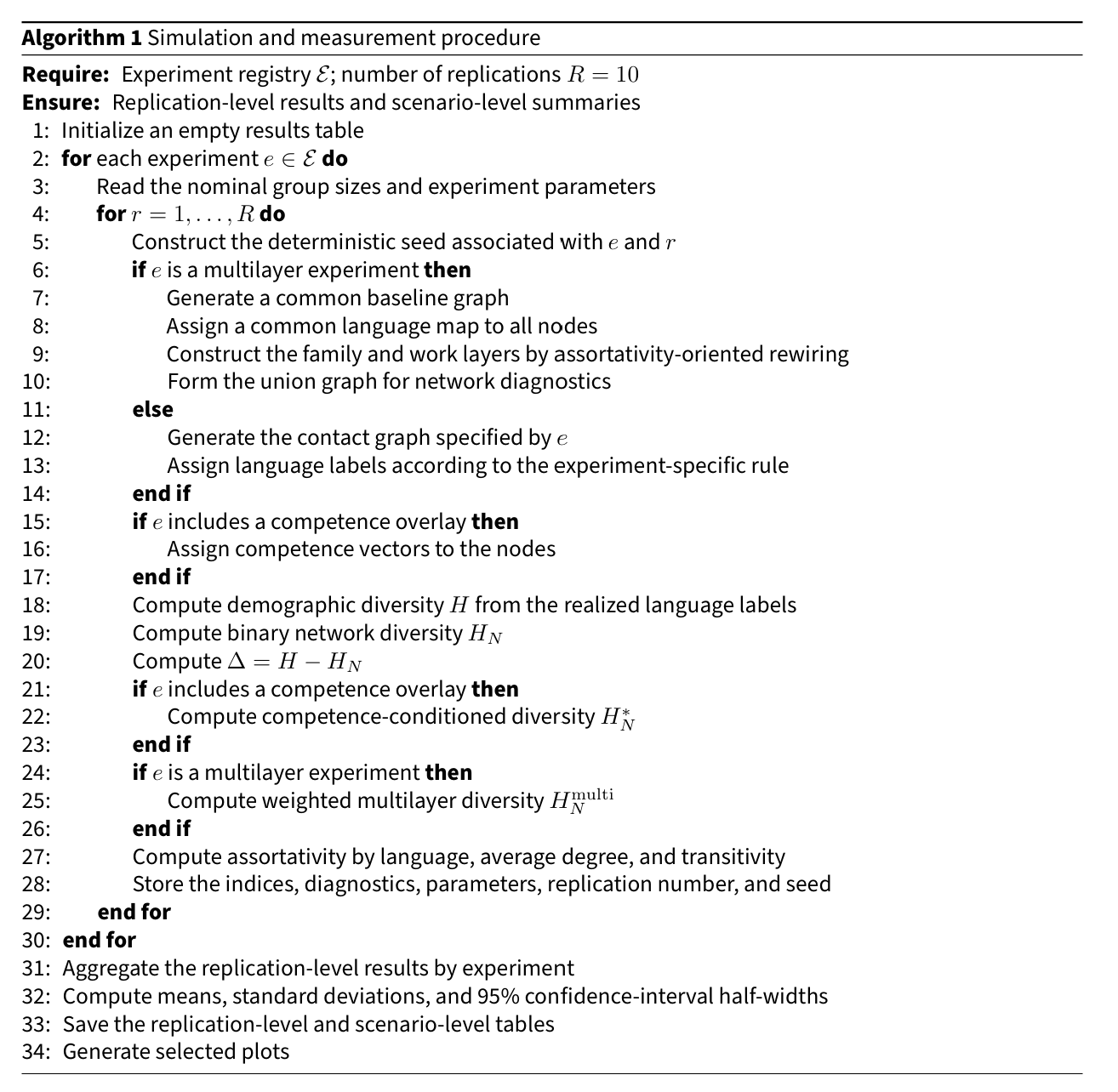
Outputs
Following the procedure summarized in Algorithm 1, the script produces two principal tabular outputs. The first is a long-format file containing one row for each experiment and replication, including the diversity indices, network diagnostics, replication number, and random seed. The second is a scenario-level summary file reporting the mean, standard deviation, and normal-approximation 95% confidence-interval half-width for each available measure.
The current output files are:
model_outputs/archetype_results_long_9.csv;model_outputs/archetype_results_summary_9.csv.
The script also generates the competence-conditioned plot showing \(H_N^*\) across second-language competence levels and a diagnostic core–periphery plot. The saved tabular outputs provide the numerical results used to construct the simulation tables and the remaining visualizations discussed in the paper.
Footnotes
- For a detailed discussion of the Greenberg index, its interpretation, and its limitations, see Civico (2026).↩︎
- The stochastic block model is a standard random-graph model in which the population is partitioned into groups and each potential edge is placed independently with a probability that depends only on the group memberships of its endpoints. See Holland et al. (1983) for the original formulation and Abbe (2018) for a more recent overview.↩︎
- The small difference arises because the stochastic block model specifies edge probabilities \(a\) and \(b\) rather than fixed counts. As a result, the expected total number of edges slightly differs from the imposed value (\(|E|=20\)), making the expected cross-edge fraction \(\mathbb{E}[H_N]\approx 0.238\) instead of exactly \(0.2\). For a proof see Appendix A.↩︎
- The complete proof is provided in Appendix B.↩︎
- This is only one possible stylized configuration. The reverse pattern also occurs empirically. In Ireland, for example, stronger Irish-language use is concentrated in peripheral Gaeltacht areas rather than in the main urban centres. In the canton of Grisons, Romansh is traditionally associated with peripheral valleys such as the Engadin, the Val Müstair, Central Grisons, and the Surselva, while the main urban centre of Chur is predominantly German-speaking. More generally, the point of the archetype is not to reproduce a universal empirical regularity, but to isolate the effect of placing linguistic heterogeneity in structurally different parts of the network.↩︎
- The reader may notice that this concept is closely related to the previously discussed notion of homophily. The two are not identical, however: homophily is the broader sociological concept referring to the tendency of similar individuals to associate, whereas assortativity is its network-level statistical expression, summarizing the extent to which ties are concentrated among nodes sharing the same attribute.↩︎
- For reproducibility, the full implementation of these steps is documented in Appendix C. The simulation code specifies all network generators, index functions, diagnostic measures, parameter settings, random seeds, replications, and output files. The purpose of the simulations is diagnostic rather than empirical: the models are designed to isolate how different contact structures affect the relationship between demographic diversity and contact diversity.↩︎
- For each value of \(\alpha_{\mathrm{family}}\), the simulations generate independent realizations of the family and work layers from the same stochastic design. The comparison across values of \(\alpha_{\mathrm{family}}\) should therefore be interpreted as a comparison of average outcomes under the same generative assumptions and different domain weights, rather than as a reweighting of one fixed pair of layers.↩︎
References
ABBE, E. (2018). Community detection and stochastic block models: Recent developments. Journal of Machine Learning Research, 18(177), 1–86.
ALESINA, A., & Zhuravskaya, E. (2011). Segregation and the quality of government in a cross-section of countries. American Economic Review, 101(5), 1872–1911. [doi:10.1257/aer.101.5.1872]
BAXTER, G. J., Blythe, R. A., Croft, W., & McKane, A. J. (2009). Modeling language change: An evaluation of Trudgill’s theory of the emergence of New Zealand English. Language Variation and Change, 21(2), 257–296. [doi:10.1017/s095439450999010x]
BECKNER, C., Blythe, R., Bybee, J., Christiansen, M. H., Croft, W., Ellis, N. C., Holland, J., Ke, J., Larsen-Freeman, D., & Schoenemann, T. (2009). Language is a complex adaptive system: Position paper. Language Learning, 59(s1), 1–26.
BELLINI, E., Ottaviano, G. I. P., Pinelli, D., & Prarolo, G. (2013). Cultural diversity and economic performance: Evidence from european regions. In R. Crescenzi & M. Percoco (Eds.), Geography, Institutions and Regional Economic Performance (pp. 121–141). Springer. [doi:10.1007/978-3-642-33395-8_7]
BREDTMANN, J., Otten, S., & Vonnahme, C. (2021). Linguistic diversity in the classroom, student achievement, and social integration. Education Economics, 29(2), 121–142. [doi:10.1080/09645292.2020.1866499]
BUZATO, D., & Cunha, E. (2024). Agent-based modeling of language change in a small-world network.
CASTELLÓ, X., Loureiro-Porto, L., & San Miguel, M. (2013). Agent-based models of language competition. International Journal of the Sociology of Language, 2013(221), 21–51.
CHARALAMBOUS, C., Sánchez, D., & Toral, R. (2023). Language dynamics within adaptive networks: An agent-based approach of nodes and links coevolution. Frontiers in Complex Systems, 1, 1304448. [doi:10.3389/fcpxs.2023.1304448]
CHEVALIER, A., Isphording, I. E., & Lisauskaite, E. (2020). Peer diversity, college performance and educational choices. Labour Economics, 64, 101833. [doi:10.1016/j.labeco.2020.101833]
CIVICO, M. (2026). Measuring linguistic diversity: Limits and extensions of the Greenberg index. Journal of Quantitative Linguistics, 33(2), 117–144. [doi:10.1080/09296174.2025.2567699]
COLEMAN, J. S. (1958). Relational analysis: The study of social organizations with survey methods. Human Organization, 17(4), 28–36. [doi:10.17730/humo.17.4.q5604m676260q8n7]
CUARTERO, M., Rossi, E., Navarro, E., & Pascual y Cabo, D. (2023). Mind the net! Unpacking the contributions of social network science for heritage and bilingualism research. Research Methods in Applied Linguistics, 2(1), 100041. [doi:10.1016/j.rmal.2023.100041]
EAGLE, N., Macy, M., & Claxton, R. (2010). Network diversity and economic development. Science, 328(5981), 1029–1031. [doi:10.1126/science.1186605]
FONTAN, A., Ratta, M., & Altafini, C. (2024). From populations to networks: Relating diversity indices and frustration in signed graphs. PNAS Nexus, 3(2), pgae046. [doi:10.1093/pnasnexus/pgae046]
GAZZOLA, M., Templin, T., & McEntee-Atalianis, L. J. (2020). Measuring diversity in multilingual communication. Social Indicators Research, 147(2), 545–566. [doi:10.1007/s11205-019-02161-5]
GREENBERG, J. H. (1956). The measurement of linguistic diversity. Language, 32(1), 109–115.
GRIN, F. (2003). Diversity as paradigm, analytical device, and policy goal. In W. Kymlicka & A. Patten (Eds.), Language Rights and Political Theory (pp. 169–188). Oxford University Press. [doi:10.1093/oso/9780199262908.003.0007]
GRIN, F., & Fürst, G. (2022). Measuring linguistic diversity: A multi-level metric. Social Indicators Research, 164(2), 601–621. [doi:10.1007/s11205-022-02934-5]
GULLIFER, J. W., & Titone, D. (2020). Characterizing the social diversity of bilingualism using language entropy. Bilingualism: Language and Cognition, 23(2), 283–294. [doi:10.1017/s1366728919000026]
HOLLAND, P. W., Laskey, K. B., & Leinhardt, S. (1983). Stochastic blockmodels: First steps. Social Networks, 5(2), 109–137. [doi:10.1016/0378-8733(83)90021-7]
HRUSCHKA, D. J., Christiansen, M. H., Blythe, R. A., Croft, W., Heggarty, P., Mufwene, S. S., Pierrehumbert, J. B., & Poplack, S. (2009). Building social cognitive models of language change. Trends in Cognitive Sciences, 13(11), 464–469. [doi:10.1016/j.tics.2009.08.008]
INIESTA, A., Yang, M., Beatty-Martínez, A. L., Itzhak, I., Gullifer, J. W., & Titone, D. A. (2025). Leveraging social network data to ground multilingual background measures: The case of general and socially based language entropy. Canadian Journal of Experimental Psychology, 79(1), 15–27. [doi:10.1037/cep0000352]
KAŁAMAŁA, P., Chuderski, A., Szewczyk, J., Senderecka, M., & Wodniecka, Z. (2023). Bilingualism caught in a net: A new approach to understanding the complexity of bilingual experience. Journal of Experimental Psychology: General, 152(1), 157–174.
KRACKHARDT, D., & Stern, R. N. (1988). Informal networks and organizational crises: An experimental simulation. Social Psychology Quarterly, 123–140. [doi:10.2307/2786835]
LOUF, T., Sánchez, D., & Ramasco, J. J. (2021). Capturing the diversity of multilingual societies. Physical Review Research, 3, 043146. [doi:10.1103/physrevresearch.3.043146]
MASSEY, D. S., & Denton, N. A. (1988). The dimensions of residential segregation. Social Forces, 67(2), 281–315. [doi:10.2307/2579183]
MCPHERSON, M., Smith-Lovin, L., & Cook, J. M. (2001). Birds of a feather: Homophily in social networks. Annual Review of Sociology, 27, 415–444. [doi:10.1146/annurev.soc.27.1.415]
NEWMAN, M. E. J. (2003). Mixing patterns in networks. Physical Review E, 67(2), 026126.
OTTAVIANO, G. I. P., & Peri, G. (2006). The economic value of cultural diversity: Evidence from US cities. Journal of Economic Geography, 6(1), 9–44. [doi:10.1093/jeg/lbi002]
PUTNAM, R. D. (2007). E pluribus unum: Diversity and community in the twenty-first century. Scandinavian Political Studies, 30(2), 137–174. [doi:10.1111/j.1467-9477.2007.00176.x]
REARDON, S. F., & O’Sullivan, D. (2004). Measures of spatial segregation. Sociological Methodology, 34(1), 121–162. [doi:10.1111/j.0081-1750.2004.00150.x]
RONEN, S., Gonçalves, B., Hu, K. Z., Vespignani, A., Pinker, S., & Hidalgo, C. A. (2014). Links that speak: The global language network and its association with global fame. Proceedings of the National Academy of Sciences, 111(52), E5616–E5622. [doi:10.1073/pnas.1410931111]
ROSILLO-RODES, P., San Miguel, M., & Sánchez, D. (2023). Modeling language ideologies for the dynamics of languages in contact. Chaos, 33(11), 113117. [doi:10.1063/5.0166636]
STEELE, L. G., Bostic, A., Lynch, S. M., & Abdelaaty, L. (2022). Measuring ethnic diversity. Annual Review of Sociology, 48(1), 43–63. [doi:10.1146/annurev-soc-030420-015435]
STIRLING, A. (2007). A general framework for analysing diversity in science, technology and society. Journal of the Royal Society Interface, 4(15), 707–719. [doi:10.1098/rsif.2007.0213]
SWADESH, M. (1952). Lexico-statistic dating of prehistoric ethnic contacts: With special reference to north american indians and eskimos. Proceedings of the American Philosophical Society, 96(4), 452–463.
SWADESH, M. (1955). Towards greater accuracy in lexicostatistic dating. International Journal of American Linguistics, 21(2), 121–137. [doi:10.1086/464321]
SWADESH, M. (1971). The Origin and Diversification of Language (J. F. Sherzer, Ed.). Aldine-Atherton.
TIV, M., Kutlu, E., Gullifer, J. W., Feng, R. Y., Doucerain, M. M., & Titone, D. A. (2022). Bridging interpersonal and ecological dynamics of cognition through a systems framework of bilingualism. Journal of Experimental Psychology: General, 151(9), 2128–2143. [doi:10.1037/xge0001174]
TRIA, F., Servedio, V. D. P., Mufwene, S. S., & Loreto, V. (2015). Modeling the emergence of contact languages. PLoS One, 10(4), e0120771. [doi:10.1371/journal.pone.0120771]