Assessing Parameter Identifiability in Agent-Based Models with Bayesian Amortized Inference

aDepartment of Social and Political Sciences, University of Milan, Italy
Journal of Artificial
Societies and Social Simulation 29 (4) 10
<https://www.jasss.org/29/4/10.html>
DOI: 10.18564/jasss.6393
Received: 16-Feb-2026 Accepted: 25-Oct-2026 Published: 31-Oct-2026
Abstract
Estimating the parameters of agent-based models from empirical data is of fundamental importance, as uncertainty in these estimates can expose non-identifiability issues that undermine inferences drawn from the underlying generative mechanism. This has implications for out-of-sample prediction, policy recommendations, and decision-making. In this study, we present an amortized Bayesian parameter estimation pipeline based on the generative artificial intelligence framework of normalizing flows, which enables a fast and systematic assessment of parameter identifiability. This approach can be scaled efficiently across multiple datasets and can be used for both rapid theory testing and computationally intensive Bayesian diagnostics, including parameter recoverability tests and simulation-based calibration. Using the Python packageBayesFlow, we demonstrate the pipeline using two illustrative models: one from opinion dynamics and one from infectious disease modelling. Furthermore, we provide a general introduction to BayesFlow for agent-based models, integrating identifiability assessment into a comprehensive Bayesian workflow and emphasizing its significance at every stage of the inference process.
Introduction
Agent-based models (ABMs) can serve a wide range of purposes (Edmonds et al. 2019), among which explanation is particularly important. By taking advantage of the flexibility and expressivity of programming languages, researchers across disciplines use ABMs to implement, in an explicit and procedural manner, the logical steps of a theory intended to account for a phenomenon of interest (Cranmer et al. 2020; Epstein 2008; Renzini et al. 2023). Starting from a set of input ingredients – agents, their attributes, behavioral rules, and initial conditions – modelers specify how these components interact and combine, through action and scheduling protocols, to generate outcomes of interest (Epstein 2006; Epstein 2008). Therefore, ABMs "grow" or algorithmically construct macro-level phenomena from the interactions between hypothesized micro-level constituents (Borrill & Tesfatsion 2011; Epstein 2006; Manzo 2022).
The scientific relevance of an explanation implemented within an ABM ultimately depends on the degree to which simulation outputs can be meaningfully related to the corresponding empirical observables (Collins et al. 2024; Edmonds et al. 2019; Epstein 2006; Grimm et al. 2005; Hines et al. 2014; Lux & Zwinkels 2018). This process typically involves algorithms that systematically explore the model’s parameter space to identify the combination of parameters that minimize a specified distance between simulated and observed outcomes (Hines et al. 2014; Lueckmann et al. 2017; Shan & Wang 2010).
A wide range of approaches has been proposed to this end (Carrella 2021; Hazelbag et al. 2020; Platt 2020), including genetic algorithms (Reuillon et al. 2015; Stonedahl & Wilensky 2010; Thiele et al. 2014), simulated annealing (Thiele et al. 2014), particle swarm optimization (Michels et al. 2022; Vlad et al. 2024), the method of simulated moments (Franke 2009; Platt 2020), Nelder-Mead (Hunter & Duggan 2025; Platt & Gebbie 2018), and gradient-based methods (Kotthoff & Hamacher 2022). All are heuristic in nature: their performance depends on the specific characteristics of the model and data, implying that no single search algorithm performs optimally across all possible ABMs for a given set of empirical observables (Carrella 2021).
These approaches also share a more fundamental limitation: they recover only a single parameter combination that best matches simulation outputs to empirical data, without natively providing estimates of the uncertainty associated with that solution (Hines et al. 2014; Lueckmann et al. 2017; McCulloch et al. 2022; Poole & Raftery 2000; Robertson et al. 2025). This matters because multiple parameter combinations may fit the data equally well – a situation that gives rise to non-identifiability, whereby the available data are insufficient to distinguish reliably between alternative parameterizations and, consequently, between the competing theoretical explanations they imply (Daly et al. 2018; Hines et al. 2014; Preston et al. 2025; Rannala 2002; Rothenberg 1971; Wechsler et al. 2013).
For instance, in a model of financial markets, non-identifiability would arise if the observed asset price data were equally consistent with retail investors being highly risk-averse or highly risk-taking, preventing researchers from determining which behavioral regime actually generated the observed patterns, given the model’s specification and level of detail. Inferences drawn from such ambiguous estimates may therefore be misleading or incorrect, potentially resulting in flawed model-based predictions or decisions (Alarid-Escudero et al. 2018; Preston et al. 2025; Raue et al. 2009; Semochkina & Walsh 2025; Siekmann et al. 2012; Villaverde 2019). Indeed, although both parameterizations may reproduce historical price movements equally well, they could imply substantially different market responses to future events. For example, a sudden increase in market uncertainty might trigger widespread selling and a sharp price decline under one parameterization, while producing a more moderate response under the other. Similarly, a policy intervention, such as a temporary restriction on trading, might stabilize prices under one parameterization but have little effect, or even amplify volatility, under another.
Assessing non-identifiability therefore requires search algorithms that explore the model’s parameter space while explicitly quantifying uncertainty in the parameter values that best reproduce the empirical data (Hines et al. 2014; McCulloch et al. 2022; Olukan et al. 2026; Poole & Raftery 2000; Preston et al. 2025; Raue et al. 2009). Such algorithms make it possible to characterize the full range of parameter values consistent with the observations and to determine whether the resulting uncertainty primarily reflects stochasticity and noise in model evaluation or instead indicates deeper structural identifiability problems. In the latter case, the modeler may need to reconsider key assumptions, incorporate additional data, or revise the model itself (Anstett-Collin et al. 2020; Daly et al. 2018; Olukan et al. 2026; Preston et al. 2025).
A Bayesian approach provides a natural framework for quantifying uncertainty and assessing identifiability in ABM parameter estimates (Olukan et al. 2026). Rather than a single point estimate, Bayesian inference yields a posterior distribution for each parameter, along with their joint distributions, encoding everything the data reveal about the plausible range of model parametrizations (Hines et al. 2014; Lam et al. 2022; Lueckmann et al. 2017; Semochkina & Walsh 2025; Siekmann et al. 2012). In this work, we present a Bayesian pipeline for parameter estimation and uncertainty quantification for agent-based models based on normalizing flows (Kobyzev et al. 2020; Papamakarios et al. 2021; Rezende & Mohamed 2015), following the approach originally introduced by Radev et al. (2020). This pipeline enables a fast and systematic assessment of parameter identifiability.
The core idea behind normalizing flows is that an arbitrarily complex target distribution can be represented as a sequence of non-linear, bijective transformations of a simple latent distribution (e.g., a standard Gaussian), from which sampling is straightforward (Rezende & Mohamed 2015). This principle has influenced much of the recent progress in generative artificial intelligence (Kobyzev et al. 2020). In the context of Bayesian inference, it recasts approximating the posterior distribution of model parameters given observations as the problem of learning an invertible mapping between a simple latent distribution and the target posterior, a task implemented using appropriate neural architectures (Dyer et al. 2024; Min et al. 2026), such as a conditional invertible neural network (cINN) (Radev et al. 2020). Once trained, these architectures enable computationally inexpensive, amortized posterior inference for new observations, making it possible to conduct systematic parameter identifiability assessments through recoverability tests (Betancourt 2020). More generally, they also facilitate the efficient application of computationally intensive Bayesian diagnostics, such as simulation-based calibration (SBC) and posterior contraction, to assess posterior quality and the extent to which the data constrain parameter uncertainty (Betancourt 2020; Talts et al. 2018).
Building on these capabilities, we implement a complete estimation pipeline in which the assessment of identifiability is central throughout the inference process, using the BayesFlow Python package (Kühmichel et al. 2026; Radev et al. 2023). We apply it to two case studies: (i) a version of the bounded confidence opinion dynamics model of Hegselmann & Krause (2002), featuring agents with heterogeneous bounds of confidence as proposed by Lorenz (2012); and (ii) a susceptible–infected–recovered (SIR) model of infectious disease spread, extended to account for reporting delays and noisy observations of infected and recovered cases (Radev et al. 2021).
In the first case study, agents hold an opinion on a topic of public interest and are subject to peer influence, dynamically updating their views by assimilating the mean opinion of individuals they consider sufficiently similar to themselves — namely, those falling within their bound of confidence. We show how BayesFlow can be used to infer posterior distributions over the maximum bound of confidence from observed opinion distributions across different groups, and to assess whether, and under which conditions, this parameter can be identified from opinion data. In the second case study, agents have an equal probability of encountering every other agent in a population, from whom they may contract a disease with a specified probability of infection, and from which they may subsequently recover with a specified recovery probability. Observations on cases are assumed to arrive with a reporting delay. We jointly estimate the parameters governing transmission dynamics and the reporting delay from the resulting delayed epidemic curves, examining the non-identifiability of certain parameters, proposing solutions, and discussing potential remedies when the problem cannot be resolved.
The remainder of the manuscript is organized as follows. Section 2 formulates the parameter estimation problem for ABMs, develops the Bayesian framework, and briefly surveys alternative computational Bayesian methods, highlighting the limitations that hinder comprehensive and fast identifiability checks. Section 3 describes the estimation framework based on normalizing flows, following Radev et al. (2020). Sections 4 and 5 apply this framework using the BayesFlow Python package (Kühmichel et al. 2026; Radev et al. 2023) to the two illustrative toy examples. Finally, Section 6 discusses limitations and outlines directions for future research.
Parameter Estimation in Agent-Based Models
Preliminaries: Intractable likelihoods
An agent-based model can be formalized as an arbitrarily complex function or generative mechanism \(g(\cdot)\), which maps a set of inputs to outputs (Carrella 2021; Epstein 2006; Hooten et al. 2020; Poole & Raftery 2000).1 The inputs to \(g(\cdot)\) are parameters, which can be classified into two non-overlapping classes (Calvez & Hutzler 2005; Payette 2024). The first, denoted by \(\Theta\), represents the space of all behavioral parameters, consisting of \(D\)-dimensional numeric vector elements \(\theta \in \Theta\) with \(D \geq 1\), which directly govern agents’ choices.2 The second comprises model design parameters \(\zeta = (\Sigma, \Gamma, Z_{0}, \Omega)\), encompassing scheduling rules \(\Sigma\), stopping conditions \(\Gamma\), initial conditions \(Z_{0}\), and stochastic elements \(\Omega\) (Chapron et al. 2026; Cranmer et al. 2020; Payette 2024).
The output of the generative mechanism, denoted as \(\boldsymbol{x}\), can take highly expressive and potentially complex forms (Carrella 2021). These may include time series, network structures (e.g., Renzini 2025), distributions of attributes within the artificial population, spatial patterns (e.g., Gunaratne et al. 2023), or even textual data (e.g., Betz 2022). Putting everything together, an agent-based model can be formalized as the following mapping:
| \[ g: (\theta, \sigma, \gamma, z_{0}, \omega) \mapsto \boldsymbol{x}\] | \[(1)\] |
Now suppose we observe \(\boldsymbol{x^{*}}\), the empirical counterpart of \(\boldsymbol{x}\). Our goal is to identify parameter combinations that produce simulated outputs closely matching \(\boldsymbol{x^{*}}\), while quantifying the associated parameter uncertainty in order to diagnose potential non-identifiability issues (Raue et al. 2009). A conventional statistical approach would define a likelihood function, maximize it, and use the Fisher information matrix to quantify this uncertainty (Brehmer 2021; Carrella 2021; Cowan 2013; Rothenberg 1971; Snijders et al. 2010). Since inferential interest typically centers on behavioral parameters \(\theta\) rather than design components \(\zeta\) (Berger et al. 1999; Payette 2024; Shiono 2021), an ideal strategy would treat \(\zeta\) as a nuisance and marginalize over all of its elements (Berger et al. 1999; Cranmer et al. 2020; Kühmichel et al. 2026; Louppe 2026; Rezende & Mohamed 2015). The resulting marginal likelihood would evaluate how well a given behavioral specification explains the observed data, averaged over all possible design specifications. In practice, however, evaluating this quantity is computationally intractable. The high dimensionality of \(\zeta\), together with the analytical complexity of \(g(\cdot)\) in most ABMs, precludes direct evaluation (Banks & Hooten 2021; Brehmer 2021; Cranmer et al. 2020; Louppe 2026).
The intractability of the marginal likelihood does not, however, preclude inference altogether. Diggle & Gratton (1984) recognized that running \(g(\cdot)\) is equivalent to drawing samples from an implicit likelihood function that cannot be evaluated in closed form (Deistler et al. 2025; Gutmann & Corander 2016; Kühmichel et al. 2026). This insight laid the foundations of simulation-based inference (SBI) (Cranmer et al. 2020). Although Diggle & Gratton (1984) adopted a frequentist perspective, Bayesian formulations have since become predominant in SBI (Deistler et al. 2025; Kühmichel et al. 2026; Lueckmann et al. 2017) — and it is within this Bayesian SBI framework that the approach presented in this paper operates.
The Bayesian approach
The posterior distribution of the \(D\)-dimensional parameter vector \(\theta = (\theta_1, \theta_2, \dots, \theta_D)\) given the observed data \(\boldsymbol{x}^*\), denoted \(p(\theta \mid \boldsymbol{x}^*)\), characterizes all parameter combinations – along with their inter-parameter dependencies and correlations – that are compatible with the observations according to the model, and quantifies their relative plausibility or weight under the posterior. Once a posterior has been estimated, we can therefore assess whether the parameter values compatible with the data point to a single, behaviorally coherent generative mechanism, or whether several distinct theoretical explanations encoded in the parameters remain plausible, with the posterior weighting each explanation by its relative probability.
A Bayesian estimation process begins with prior distributions, which encode initial beliefs and guide the exploration of the behavioral parameters space (Deistler et al. 2025). In the following, we assume that estimation is conditional on a fixed specification of \(\zeta\). Each forward simulation of the model is then executed with its own random seed (Kühmichel et al. 2026). For simplicity, and without loss of generality, we omit this conditioning from the equations presented below.
Our inferential target is therefore:
| \[ p(\theta \mid \boldsymbol{x^{*}}) = \frac{p (\boldsymbol{x^{*}} \mid \theta) \; p(\theta)}{p(\boldsymbol{x^{*}})} = \frac{p (\boldsymbol{x^{*}} \mid \theta) \; p(\theta)}{\int_{\Theta} p (\boldsymbol{x^{*}} \mid \theta) \; p(\theta) \; d\theta}\] | \[(2)\] |
Building on the insight of Diggle & Gratton (1984), simulation-based methods can be used to approximate the posterior distribution, or key moments thereof, without directly evaluating the likelihood. Parameters are drawn from the prior and used to run forward simulations, generating synthetic datasets \(\boldsymbol{x}\). The resulting pairs of prior-sampled parameters and corresponding simulation outputs constitute joint draws from the prior predictive distribution (Raynal et al. 2019), formally expressed as \((\theta, \boldsymbol{x}) \sim p(\boldsymbol{x} \mid \theta)\, p(\theta) = p(\boldsymbol{x}, \theta) = p(\theta, \boldsymbol{x})\).
These samples can be exploited in two broad ways (Min et al. 2026). The first applies a filtering or acceptance criterion to retain only those parameter combinations that generate outputs sufficiently close to the observed data \(\boldsymbol{x}^{*}\) (Carrella 2021; Cranmer et al. 2020; Gutmann & Corander 2016). By discarding implausible parameter draws, this procedure updates the prior in light of the observations, yielding an approximation to the joint posterior distribution \(p(\theta \mid \boldsymbol{x}^{*})\) without explicitly evaluating the likelihood. The approximation can be progressively refined through importance sampling techniques (Sisson et al. 2007; Toni et al. 2009). The second approach leverages machine-learning algorithms to learn the relationship between simulated outputs and each individual parameter in \(\theta\) within the prior predictive samples. The learned mapping is then applied to the observed data \(\boldsymbol{x}^{*}\) to approximate the marginal posterior and relevant posterior summaries (Raynal et al. 2019).
Computational Bayesian techniques
Approximate Bayesian Computation - Sequential Monte Carlo (ABC-SMC) is one of the most widely used methods in the modelling community for implementing the first approach (Beaumont 2019; Csilléry et al. 2010; Gozzi et al. 2025; McCulloch et al. 2022; Olukan et al. 2026; Schälte et al. 2022; Sisson et al. 2007; Toni et al. 2009). Starting from the prior distributions, parameters are repeatedly sampled and the model is simulated until \(\rho\) parameter combinations (e.g., \(\rho = 100\)) that generate simulated outputs sufficiently close to the observed data are found. Closeness is assessed via a tolerance threshold \(\tau_{1}\), such that retained parameters satisfy \(d(\boldsymbol{x}, \boldsymbol{x^{*}}) \leq \tau_1\), for a user-defined distance function \(d(\cdot, \cdot)\). In practice, however, it is rarely feasible to compare raw outputs and observations directly. Instead, inference is typically performed on a set of summary statistics \(S(\cdot)\) computed on both simulated and observed data. The acceptance criterion therefore becomes \(\hat{d}(S(\boldsymbol{x}), S(\boldsymbol{x^{*}})) \leq \tau_1\), which effectively filters the prior distribution by retaining only those \(\rho\) parameter combinations that generate simulated summaries sufficiently close to their empirical counterparts under a canonical \(\hat{d}(\cdot, \cdot)\).
At this stage, we obtain a first approximation of the joint posterior density by filtering the prior using empirical evidence. Unless the tolerance \(\tau_{1}\) is already very small, this approximation is generally coarse. Moreover, imposing a very strict tolerance threshold from the outset – corresponding to pure ABC rejection sampling – is computationally prohibitive in most practical applications (Cranmer et al. 2020). A more efficient strategy is therefore to start with a relatively large tolerance and progressively refine the approximation through a sequence of intermediate distributions (Sisson et al. 2007; Toni et al. 2009).
Specifically, subsequent approximations are generated by sampling parameters from the current approximation of the posterior with associated importance weights3 and then perturbing the sampled parameters using a kernel – most commonly a Gaussian kernel (Sisson et al. 2007) – to promote local exploration of the parameter space. Let \(\theta^{\prime}\) denote a parameter vector sampled from the first posterior approximation, and let \(\theta^{\prime\prime}\) denote the perturbed parameter obtained after applying the kernel. The perturbed parameter \(\theta^{\prime\prime}\) is then used as input to \(g(\cdot)\) to produce simulated data. If \(\theta^{\prime\prime}\) yields simulated summaries satisfying \(\hat{d}(S(\boldsymbol{x}), S(\boldsymbol{x^{*}})) \leq \tau_2\), with \(\tau_2 < \tau_1\), then \(\theta^{\prime\prime}\) is retained to form the second, refined approximation of the posterior distribution (Toni et al. 2009). This procedure is iterated over a sequence of decreasing tolerance thresholds \({\tau_1 > \tau_2 > \dots > \tau_N}\), until a target precision \(\tau_N\) is reached or a predefined computational budget is exhausted.
In the limit \(\tau_{N} \rightarrow 0\) and when \(S(\cdot)\) consists of sufficient summary statistics, the ABC-SMC approximation converges to the true posterior distribution (Cranmer et al. 2020; Sisson et al. 2007). In practice, however, reaching this limit can be computationally prohibitive. As the tolerance \(\tau\) becomes increasingly small, the probability of accepting parameter proposals from the previous approximation of the posterior rapidly vanishes, especially when \(S(\cdot)\) is high-dimensional (Cranmer et al. 2020). Moreover, this entire procedure must be repeated from scratch for every new dataset \(\boldsymbol{x}^{*,\prime}\), whether it comes from a different empirical setting or is generated synthetically for diagnostic checks, including parameter recoverability tests for diagnosing non-identifiability and simulation-based calibration (SBC) for assessing the overall quality of the estimated posterior (Betancourt 2020; Kühmichel et al. 2026; Radev et al. 2020; Talts et al. 2018).
For instance, recoverability tests for assessing parameter identifiability check whether the model can systematically recover its own parameters. This typically involves fixing a ground truth parameter combination, generating synthetic data from it, and fitting the model to these data to verify that the estimated posterior places sufficiently high probability mass near the original parameters (Betancourt 2020; Carrella 2020; van Ravenzwaaij & Oberauer 2009). Because this check must be repeated across many ground truth combinations, an ABC-SMC framework, such as the one proposed by Olukan et al. (2026), becomes prohibitively expensive, since each repetition requires a new, costly search to gradually transform the prior into an approximation of the posterior (Kühmichel et al. 2026; Radev et al. 2020). Beyond these computational considerations, the reliability of the identifiability diagnosis itself depends critically on the choice of the summary statistics \(S(\cdot)\), the distance function \(d(\cdot,\cdot)\), and the sequence of tolerance thresholds \(\tau_1 > \tau_2 > \dots > \tau_N\).
Raynal et al. (2019) introduced ABC-Random Forest (ABC-RF), one of the most prominent methods of the second approach. The method consists of drawing a sufficiently large number of samples from the prior predictive distribution and using random forest (RF) techniques to learn the nonlinear relationships between a set of summary statistics \(S(\cdot)\) computed from \(\boldsymbol{x}\), which serve as predictors, and each of the corresponding generating parameter values sampled from the prior, which constitute the prediction targets. Since RF techniques are robust to the inclusion of irrelevant predictors, ABC-RF can accommodate an arbitrarily large number of summary statistics, including non-informative ones, thereby effectively eliminating the need for careful manual selection of informative summaries (Collin et al. 2021; Raynal et al. 2019).
Once an accurate mapping is learned, any dataset \(\boldsymbol{x}^{*,\prime}\) can be compressed into \(S(\boldsymbol{x}^{*,\prime})\) and passed to the trained RF to obtain a marginal posterior distribution for the corresponding parameter (typically reported via its posterior mean and credible intervals; Raynal et al. 2019), without the need to specify distance functions or tolerance thresholds (Collin et al. 2021; Raynal et al. 2019). Crucially, the mapping is learned only once and can subsequently be applied to any new dataset at negligible computational cost — a property known as amortization, which shifts the computational burden to an upfront training phase and makes subsequent inference extremely efficient (Radev et al. 2020). For this reason, parameter recoverability tests that diagnose non-identifiability issues and SBC are also straightforward to perform (Betancourt 2020; Raynal et al. 2019; Talts et al. 2018).
However, because a separate forest is typically trained independently for each parameter \(\theta_{j} \in \theta\), ABC-RF only returns univariate marginal posterior distributions (Raynal et al. 2019), and does not directly provide the full joint posterior distribution capturing the dependencies between parameters. This limitation is particularly relevant for identifiability analysis, as joint posterior distributions can reveal strong parameter dependencies, which are often encountered in agent-based models. These may manifest as ridges or curved high-density regions in parameter space, along which different parameter combinations explain the observed data comparably well (Betancourt 2020; Daly et al. 2018; Hines et al. 2014; Olukan et al. 2026; Preston et al. 2025; Raue et al. 2009). Such patterns indicate that the data identify only certain combinations of parameters (e.g., their sum or ratio), so that several behaviorally distinct generative mechanisms may remain plausible. Marginal posteriors alone discard this information and can conceal these dependencies among parameters.
Moreover, while ABC-RF avoids explicit feature selection, it still relies on user-defined summary statistics derived from domain intuition, which may fail to capture subtle higher-order patterns or information-dense moments present in raw data (Min et al. 2026).
The BayesFlow pipeline presented here combines the key advantages of these two approaches. It approximates the full multivariate joint posterior distribution, explicitly capturing inter-parameter dependencies and correlations that are essential for identifiability analysis, while eliminating the need for hand-crafted summary statistics by learning informative embeddings directly from raw, multi-dimensional data. Because inference is amortized after an upfront training phase, the pipeline can be readily applied to new datasets at minimal computational cost. This makes near-instantaneous parameter recoverability tests for identifiability analysis feasible, while also making the broader suite of Bayesian diagnostic checks practical to perform at scale.
Bayesian Estimation via Normalizing Flows
The core idea
Following the framework introduced by Rezende & Mohamed (2015) and further developed by Radev et al. (2020), suppose that we have a parametrized function \(f_{\phi}(\cdot)\), with parameters \(\phi\), that defines a bijective and differentiable mapping between \(D\)-dimensional vectors4 in \(\mathbb{R}^{D}\). The inverse mapping \(f_{\phi}^{-1} : \mathbb{R}^{D} \to \mathbb{R}^{D}\) therefore exists and uniquely recovers the input vector from the output.
We generate pairs of observations \((\theta, \boldsymbol{x}) \sim p(\boldsymbol{x} \mid \theta)\, p(\theta)\) (Radev et al. 2021), where \(\theta \in \Theta \subseteq \mathbb{R}^{D}\). Simulations are performed conditional on a fixed specification of \(\zeta\), as discussed above, with the exception of the random seed (Kühmichel et al. 2026). We then provide \(f_{\phi}(\cdot)\) with the sampled parameter values \(\theta\), with the goal of transforming each \(D\)-dimensional vector of behavioral parameters into a \(D\)-dimensional latent variable \(\boldsymbol{z}\), assumed to follow a multivariate standard Gaussian distribution with zero mean and unit covariance matrix, that is, \(\boldsymbol{z} \sim \mathcal{N}(\boldsymbol{0}, \mathbf{I}_D)\). The transformation from \(\theta\) to \(\boldsymbol{z}\) is data-dependent, in the sense that the corresponding simulated observations \(\boldsymbol{x}\) are used to modulate the parameters of the invertible mapping (Radev et al. 2020).
The parameters \(\phi\) are tuned so that, for a given simulated output \(\boldsymbol{x}'\), the forward transformation \(f_{\phi}(\theta^{\prime}, \boldsymbol{x}')\) defines a bijection between the parameter space \(\Theta \subseteq \mathbb{R}^{D}\) and the latent space. For a particular parameter vector \(\theta^{\prime}\) that generated \(\boldsymbol{x}^{\prime}\), this mapping yields a corresponding latent representation \(\boldsymbol{z}^{\prime}\), i.e.,
| \[ \boldsymbol{z}^{\prime} = f_{\phi}(\theta^{\prime},\boldsymbol{x}^{\prime})\] | \[(3)\] |
By invertibility, the original parameter vector should be recovered exactly via the inverse transformation,
| \[ \theta^{\prime} = f_{\phi}^{-1}(\boldsymbol{z}^{\prime}, \boldsymbol{x}^{\prime})\] | \[(4)\] |
The key idea is that, if a sufficiently accurate mapping \(f_{\phi}(\cdot)\) can be learned using only samples \((\theta, \boldsymbol{x})\) from the prior predictive distribution, then posterior inference for an empirical observation \(\boldsymbol{x}^{*}\) becomes straightforward. In particular, we obtain an approximation \(p_{\phi}(\theta \mid \boldsymbol{x}^{*})\) to the true posterior \(p(\theta \mid \boldsymbol{x}^{*})\) by (i) sampling \(L\) latent vectors \(\boldsymbol{z}_{\ell}\) from the multivariate standard Gaussian distribution, (ii) passing each \(\boldsymbol{z}_{\ell}\) together with \(\boldsymbol{x}^{*}\) through the inverse transformation, and (iii) recovering the corresponding parameter samples \(\{\theta_{\ell}\}_{\ell=1}^{L}\) via Equation 4.
Importantly, once the mapping \(f_{\phi}(\cdot)\) has been learned, this procedure can be applied independently to any number of datasets, observed or synthetic, at negligible additional computational cost (Kühmichel et al. 2026), and without re-estimating the full posterior from scratch. In essence, a normalizing flow guarantees that drawing samples from a simple multivariate standard Gaussian and mapping them back, together with \(\boldsymbol{x}^{*}\), to the parameter space via the learned inverse transformation in Equation 4 corresponds to sampling from the approximated posterior \(p_{\phi}(\theta \mid \boldsymbol{x}^{*})\).
Radev et al. (2020) implemented \(f_{\phi}(\cdot)\) using a conditional invertible neural network architecture (cINN; Dinh et al. 2016) composed of a sequence of affine coupling blocks (ACBs). Within each block, neural networks parameterize invertible scaling and shifting transformations that progressively map the \(D\)-dimensional behavioral parameter vector \(\theta\) to a latent vector \(\boldsymbol{z}\), with the simulated data \(\boldsymbol{x}\) provided as conditioning information in each transformation step. Further technical details are provided by Dinh et al. (2016) and Radev et al. (2020).
Learning the posterior
Once we define a neural network architecture for the invertible mapping \(f_{\phi}(\cdot)\), the next step is to learn the parameters \(\phi\) (i.e., the neural network weights) governing the transformation. The goal is to ensure that the distribution of the \(L\) behavioral parameter vectors \(\{\theta_{\ell}\}_{\ell=1}^{L}\) obtained from \(f_{\phi}^{-1}(\boldsymbol{z}_{\ell}, \boldsymbol{x}^{*})\) closely matches the true posterior distribution \(p(\theta \mid \boldsymbol{x}^{*})\).
Since sampling \(L\) latent vectors \(\boldsymbol{z}_{\ell}\) from a multivariate standard Gaussian and passing them, together with \(\boldsymbol{x}^{*}\), through the cINN in the inverse direction (Equation 4) corresponds to drawing samples directly from the approximate posterior \(p_{\phi}(\theta \mid \boldsymbol{x}^{*})\) (Radev et al. 2020), we can enforce consistency between the true, unobserved posterior and the output of the inverse pass of the normalizing flow by selecting the parameters \(\phi\) to minimize the Kullback-Leibler (KL) divergence between \(p(\theta \mid \boldsymbol{x})\) and \(p_{\phi}(\theta \mid \boldsymbol{x})\) for each possible dataset \(\boldsymbol{x}\), that is,
| \[ \hat{\phi} = \underset{\phi}{\arg\min} \; \mathbb{E}_{p(\boldsymbol{x})}\!\left[\mathbb{KL}\!\left(p(\theta \mid \boldsymbol{x}) \,\|\, p_{\phi}(\theta \mid \boldsymbol{x})\right)\right]\] | \[(5)\] |
By construction of the normalizing flow and the change-of-variables formula, \(p_{\phi}(\theta \mid \boldsymbol{x})\) can equivalently be written as:
| \[ p_{\phi}(\theta \mid \boldsymbol{x}) = p\!\left(\boldsymbol{z} = f_{\phi}(\theta, \boldsymbol{x})\right) \left|\det\!\left(\frac{\partial f_{\phi}(\theta, \boldsymbol{x})}{\partial \theta}\right)\right|\] | \[(6)\] |
Expanding Equation 5 according to the definition of the KL divergence between continuous probability distributions, substituting the change-of-variables expression for the approximate posterior from Equation 6, and approximating the resulting expectation using Monte Carlo samples generated by the simulator \(g(\cdot)\), we obtain the following optimization objective:
| \[\begin{aligned} \hat{\phi} &= \underset{\phi}{\arg\min} \; \frac{1}{M} \sum_{m=1}^{M} \left( \frac{\left\| f_{\phi}(\theta^{(m)}, \boldsymbol{x}^{(m)}) \right\|_2^2}{2} - \log \left| \det J_{f_\phi}^{(m)} \right| \right)\end{aligned}\] | \[(7)\] |
This expression results from specifying the latent variable \(\boldsymbol{z}\) to follow a standard multivariate Gaussian distribution with zero mean and unit covariance. A full derivation is provided in the Supplementary Materials.
Equation 7 defines our training loss. Minimizing this loss using standard stochastic gradient–based optimization algorithms yields parameters \(\hat{\phi}\) such that the induced latent representations follow the prescribed standard multivariate Gaussian distribution, while simultaneously learning an accurate invertible mapping between the parameter space \(\Theta\) and the latent space. This, in turn, ensures that the resulting approximate posterior is as close as possible to the true posterior over behavioral parameters given the observed data \(\boldsymbol{x^*}\).
If the training procedure converges perfectly and the stochastic gradient–based optimization algorithm identifies the true global optimum \(\hat{\phi}^{*}\) (which is unlikely in practice; see Radev et al. 2020), then the learned approximate posterior coincides with the true posterior distribution.
Adding a summary neural network
The simulated output \(\boldsymbol{x}\) may take the form of a high-dimensional data structure, such as a long multivariate time series, a social network, or a spatial map. In such cases, it is often desirable to map \(\boldsymbol{x}\) to a lower-dimensional representation, commonly referred to as an embedding, in order to accelerate training and mitigate numerical instabilities arising from redundancies in high-dimensional data (Dyer et al. 2024; Radev et al. 2020).
Crucially, however, rather than relying on hand-crafted summary statistics, we aim to learn these representations directly from data using an appropriate neural architecture (Radev et al. 2020). The goal is to obtain a lower-dimensional embedding or representation that is sufficient for inference, in the sense that it preserves all information in \(\boldsymbol{x}\) relevant for recovering the full posterior distribution over behavioral parameters.
Let us denote as \(\tilde{\boldsymbol{x}}\) the learned lower-dimensional representation of \(\boldsymbol{x}\), and as \(\tilde{\boldsymbol{x}}^{*}\) the learned lower-dimensional representation of the empirical observations. Both representations are obtained by passing \(\boldsymbol{x}\) and \(\boldsymbol{x}^{*}\) through a neural network architecture \(h_{\psi}(\cdot)\), parameterized by a set of weights \(\psi\), which are distinct from \(\phi\). Hence, we have \(\tilde{\boldsymbol{x}} = h_{\psi}(\boldsymbol{x})\) and \(\tilde{\boldsymbol{x}}^{*} = h_{\psi}(\boldsymbol{x}^{*})\). The parameters \(\psi\) are optimized jointly with the parameters of the cINN, \(\phi\), such that the complete training loss, optimized via stochastic gradient descent, is:
| \[ \hat{\phi}, \hat{\psi} = \underset{\phi, \psi}{\arg\min} \; \frac{1}{M} \sum_{m=1}^{M} \left( \frac{\left\| f_{\phi}(\theta^{(m)}, h_{\psi}(\boldsymbol{x}^{(m)}) \right\|_2^2}{2} - \log \left| \det J_{f_\phi}^{(m)} \right| \right)\] | \[(8)\] |
Proposition 2 in Radev et al. (2020) guarantees that if the optimization algorithm is able to find the true global optima \((\hat{\phi}^{*}, \hat{\psi}^{*})\), and if \(h_{\psi^{*}}(\cdot)\) learns a lossless and sufficient lower-dimensional representation of the data, then the approximate posterior \(p_{\hat{\phi}^{*}, \hat{\psi}^{*}}(\theta \mid \boldsymbol{x})\) coincides with the true posterior. If instead \(h_{\psi^{*}}(\cdot)\) fails to capture certain relevant information in the data, the resulting posterior approximation may be systematically biased, and parameters that would otherwise be identifiable from the raw data may appear as non-identifiable.
Choosing the appropriate architecture
It is therefore crucial to choose an appropriate architecture for \(h_{\psi}(\cdot)\) that respects the probabilistic symmetries inherent in the simulated and observed data (Radev et al. 2020). For example, when the input consists of a single time series, recurrent architectures such as Gated Recurrent Units (GRUs) naturally capture sequential dependencies while accommodating inputs of variable length (Chung et al. 2014). For social network data, graph neural networks may be more suitable, as they can learn embeddings of edges and node attributes jointly, if necessary (Kipf & Welling 2017; Lin et al. 2023). Table 1 provides a representative, though non-exhaustive, overview of architectures commonly employed for various data structures. Additional examples can be found in the BayesFlow documentation (BayesFlow 2026; Kühmichel et al. 2026; Radev et al. 2023). It should be noted that these architectures are typically combined with pooling layers or other flattening and bottleneck operations to project \(\boldsymbol{x}\) or \(\boldsymbol{x}^{*}\) to a lower-dimensional representation of a user-defined size.
As shown in Table 1, multiple neural architectures are available for any given data structure, each with distinct performance characteristics and different sets of trainable parameters and hyperparameters. Choosing the most suitable architecture is therefore not straightforward a priori (Radev et al. 2020). In general, we recommend adopting the following principle: start with a standard, well-validated architecture that can reasonably represent the data and introduce additional complexity only when necessary (Radev et al. 2020). In practice, this decision can typically be made only after an estimation pipeline has been applied to the ABM and identifiability checks have been performed. We follow this approach in both case studies below.
To illustrate, when encoding a univariate distribution, should one use a DeepSet or a SetTransformer? When encoding spatial data, is a convolutional architecture preferable to an attention-based mechanism? Such questions arise for virtually any data structure \(\boldsymbol{x}\) generated by an ABM, as transformer- and attention-based architectures have been developed for a broad range of data modalities (Table 1). These architectures typically require substantially more parameters and longer training times than simpler alternatives, but can offer important advantages when the data contain higher-order dependencies, complex correlations, or multi-way interactions (Kühmichel et al. 2026). In line with the principle above, we recommend starting with a standard architecture and resorting to transformer- or attention-based alternatives only if identifiability checks or other diagnostics indicate that capturing such higher-order dependencies is necessary for the inference problem at hand.
The reason is that higher-order dependencies can carry the information needed to separate parameter values, or entire regimes of the parameter space, that lower-order features cannot distinguish. A summary network that is too simple may discard this information, so that an apparent identifiability problem may reflect information lost in the summary network rather than a limitation of the data or the model. However, whether this is the case can typically be assessed only after the pipeline has been trained and evaluated.
| Data Structure | Architecture |
|---|---|
| Time series (univariate or multivariate) | Recurrent Neural Networks (RNN), such as Long Short-Term Memory (LSTM) or Gated Recurrent Unit (GRU), Temporal Convolutional Networks (TCN), Time Series Transformer. Refs: Chung et al. (2014), Jozefowicz et al. (2015), Lea et al. (2016), Staudemeyer & Rothstein Morris (2019), Wen et al. (2022), Zhang & Mikelsons (2023). |
| Spatial map or distribution | Convolutional Neural Network (CNN), Variational Auto-Encoders (VAE), Transformer-Based Architectures. Refs: LeCun et al. (1998), Kingma & Welling (2013), Dosovitskiy et al. (2020). |
| (Social) network data (graphs) | Graph Neural Networks (GNN), such as Graph Convolutional Networks (GCN), Graph Variational Auto-Encoders (GVAE), Graph Attention Network (GAT), Gated Graph Sequence Neural Network (GGS-NN). Refs: Kipf & Welling (2017), Li et al. (2017), Veličković et al. (2018), Sanchez-Lengeling et al. (2021), Dyer et al. (2022), Lin et al. (2023), Dyer et al. (2024). |
| Distributions (univariate or multivariate) | DeepSet, SetTransformer. Refs: Zaheer et al. (2018), Lee et al. (2019). |
Once a suitable architecture for \(\boldsymbol{x}\) has been selected, a second key design decision concerns network depth. Deeper networks are more expressive (Lin & Jegelka 2018), learning increasingly abstract embeddings that capture complex patterns beyond the reach of shallower architectures (Radev et al. 2020). In graph convolutional networks for social network data (Kipf & Welling 2017), for instance, each additional layer aggregates information from nodes one hop further away, so that deeper architectures encode progressively more global structural properties. This yields richer low-dimensional representations, provided depth does not induce oversmoothing (Rusch et al. 2023). However, increasing depth raises the risk of overfitting, though the online learning strategy implemented in BayesFlow5 can mitigate this risk even in deeper architectures (Radev et al. 2020). Regarding depth and other network hyperparameters, such as activation functions and dropout rates, we recommend starting with the BayesFlow default settings (BayesFlow 2026), which are grounded in best practices from the literature underlying each architecture,6 and conducting sensitivity analyses, increasing depth only if diagnostic checks demonstrate that additional model capacity is required.
Regarding the number of affine coupling blocks (ACBs) in the cINN, we again recommend following the BayesFlow defaults. Additional ACBs increase the network’s ability to represent complex distributions but also increase training time. Radev et al. (2020) found that varying the number of ACBs between 5 and 10 generally has little effect on performance or training stability.
The whole procedure in a nutshell
Algorithms 1 and 2 summarize the training and amortized inference phases of the framework introduced by Radev et al. (2020) and implemented in the Python package BayesFlow (Kühmichel et al. 2026; Radev et al. 2023).
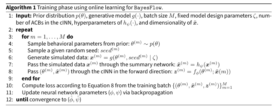
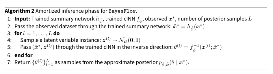
The resulting posterior enables inferential statements about the relevance of each component of the generative mechanism, as represented by the corresponding elements of \(\theta\), and facilitates the assessment of parameter non-identifiability (Bellotti et al. 2026; Daly et al. 2018; Hines et al. 2014; Olukan et al. 2026; Preston et al. 2025; Semochkina & Walsh 2025; Siekmann et al. 2012; Tang et al. 2025). For example, starting from a uniform prior that assigns equal probability to parameter values representing different generative explanations, the posterior may remain diffuse and assign non-negligible probability to parameter combinations that imply distinct agent behaviors, even when the estimation algorithm has converged (Olukan et al. 2026).
Systematic identifiability assessment and Simulation-Based Calibration (SBC)
The same procedure outlined in Algorithm 2 can also be used to assess parameter identifiability via recoverability tests and to check the fidelity of the BayesFlow estimates via SBC (Betancourt 2020; Carrella 2020; Kühmichel et al. 2026; Talts et al. 2018).
Both diagnostic pipelines begin with simulating \(N\) datasets \(\{\boldsymbol{x}^{(i)}\}_{i=1}^{N}\), obtained by passing \(N\) parameter vectors, sampled from the prior distributions, through the generative mechanism \(g(\cdot)\). The corresponding parameters used to generate each dataset are stored as “ground truth” values, \(\{\theta^{(i)}\}_{i=1}^{N}\). Each simulated dataset can then be treated as if it were an empirical observation \(\boldsymbol{x}^{*}\). For each dataset, we sample \(L\) latent vectors \(\{\boldsymbol{z}_{\ell}\}_{\ell=1}^{L}\) from the standard Gaussian, and pass them together with \(\boldsymbol{x}^{(i)}\) through the inverse transformations of the trained normalizing flow (Equation 4). This yields, almost instantaneously, \(L\) samples from the approximate posterior \(p_{\hat{\phi}, \hat{\psi}}(\theta \mid \boldsymbol{x}^{(i)})\), for each specific \(\boldsymbol{x}^{(i)}\). Because the true data-generating parameters are known, these approximate posteriors can be compared directly to the corresponding ground truth values in order to evaluate the behavior of the inference procedure.
First, we can compare the ground truth parameters \(\theta^{(i)}\) with measures of central tendency of the corresponding inferred posteriors \(p_{\hat{\phi}, \hat{\psi}}(\theta \mid \boldsymbol{x}^{(i)})\). In a well-identified model, the posterior should recover the true data-generating value \(\theta^{(i)}\) by concentrating substantial probability mass around it (Betancourt 2020). This agreement can be quantified with a variety of metrics, ranging from point-estimate errors (e.g., the raw or scaled differences between \(\theta^{(i)}\) and the posterior mean, mode, or median) to interval-based measures (e.g., whether \(\theta^{(i)}\) lies within a central posterior credible interval). In BayesFlow, this comparison is typically visualized using a bivariate scatter plot of posterior medians against the corresponding ground truth values, also reporting the posterior median absolute deviation (MAD). A Pearson correlation coefficient is then reported as a synthetic measure of the agreement between the ground truth values and the recovered posterior medians.
SBC evaluates the probabilistic integrity of the posterior as a whole. For each simulated dataset \(\boldsymbol{x}^{(i)}\), we determine the rank of the corresponding ground truth parameter \(\theta^{(i)}\) among the \(L\) posterior samples drawn from \(p_{\hat{\phi}, \hat{\psi}}(\theta \mid \boldsymbol{x}^{(i)})\), yielding a rank statistic \(r^{(i)}\). Specifically, \(r^{(i)}\) is defined as the number of posterior samples that are less than or equal to the ground truth value \(\theta^{(i)}\) extracted from the prior (Betancourt 2020; Talts et al. 2018). If the posterior coverage and uncertainty quantification are well calibrated, the distribution of rank statistics \(\{r^{(i)}\}_{i=1}^{N}\) should be approximately uniform over \(\{0,1,\dots,L\}\) (Talts et al. 2018). The theoretical foundation of this test lies in the self-consistency property of the Bayesian joint distribution. A technical derivation is provided in the Supplementary Materials.
To assess uniformity in practice, BayesFlow converts the discrete rank statistics into normalized ranks on the unit interval \([0,1]\) and computes their empirical cumulative distribution function (ECDF) across the \(N\) simulated datasets (Säilynoja et al. 2021). Rather than plotting the ECDF itself, it visualizes the ECDF difference plot, obtained by subtracting the theoretical CDF of a perfectly uniform distribution from the empirical ECDF. Under the null hypothesis of perfect calibration, the resulting curve fluctuates around zero and remains within finite-sample confidence bands (Säilynoja et al. 2021). In contrast, systematic deviations outside these bands indicate specific calibration failures or inferential pathologies (Betancourt 2020; Modrák 2025; Säilynoja et al. 2021; Talts et al. 2018). Illustrative examples of these deviation patterns, together with guidance on their interpretation, are provided in Figure S1 of the Supplementary Materials.
A Modified Bounded Confidence Model
Description
Public discourse on topics of societal importance can yield a wide spectrum of population-level opinion distributions, ranging from consensus, where most individuals share a similar position, to polarization, characterized by two opposing camps, to multipolarity, where opinions fragment into multiple distinct clusters. To explain the emergence of these collective dynamics, our first toy model simulates social interactions in which individuals exert assimilative influence on one another, adjusting their opinions accordingly (Flache et al. 2017). The model builds on the modifications proposed by Lorenz (2010, 2012) to the well-known bounded confidence model introduced by Hegselmann & Krause (2002). See also its application in Renzini & Squazzoni (2026).
We consider a population of \(A\) agents, indexed by \(i = 1, 2, \dots, A\). At time \(t = 0\), each agent holds an opinion \(o_i^{t_{0}}\) on a given topic of public interest, distributed within the unit interval \([0,1]\) according to a specified probability density function. Opinions are treated as dynamic attributes that evolve over successive time steps \(t\) until a predefined stopping condition is reached. Each agent updates their opinion considering the current opinions of other agents within a set of influencing agents, \(\nu_i^t\), which itself evolves as opinions change.
Each agent also possesses a fixed attribute, the bound of confidence \(\epsilon_i\), which remains constant throughout the simulation. Unlike in Hegselmann & Krause (2002), here \(\epsilon_i\) is heterogeneous across the population (Lorenz 2010), drawn from a specified distribution over the interval \([0,1]\). The bound of confidence acts as a filter in the opinion space, defining which agents belong to the set of influencing agents, \(\nu_i^t\), for each \(i = 1, 2, \dots, A\). Specifically, the model assumes that agents neither fully consider nor completely disregard the opinions of others within their reference population. Instead, each agent uses their bound of confidence, \(\epsilon_i\), to determine which opinions are relevant for them.
Operationally, each agent is influenced only by those agents \(j \neq i\) whose opinions differ from the agent’s current opinion \(o_i^t\) by at most \(\epsilon_i\) in either direction. In other words, agent \(i\) takes into account only those opinions that lie within \(\epsilon_i\) points above or below their own current opinion. Formally, the set of influencing agents is defined as:
| \[\nu_i^t = \{\, j \neq i : |o_j^t - o_i^t| < \epsilon_i \,\}\] | \[(9)\] |
Once the set of influencing agents \(\nu_i^t\) has been identified, each agent updates their opinion by taking the arithmetic mean of their own current opinion and the opinions of all agents in \(\nu_i^t\). Formally, the opinion update rule is given by:
| \[ o_i^{t+1} = \frac{1}{|\nu_i^t| + 1} \left( o_i^t + \sum_{j \in \nu_i^t} o_j^t \right)\] | \[(10)\] |
The bound of confidence can represent various social, psychological, or cognitive mechanisms (Renzini & Squazzoni 2026). Here, we interpret it as homophily, a social process in which individuals preferentially assimilate the opinions of like-minded peers while disregarding dissimilar ones (Bernardo et al. 2024; McPherson et al. 2001). Therefore, the magnitude of \(\epsilon_i\) reflects the strength of homophily. A lower \(\epsilon_i\) implies that agents consider and assimilate only opinions very close to their own, indicating stronger homophily. In contrast, as \(\epsilon_i\) increases, these effects weaken and agents begin to consider and assimilate opinions that are increasingly different from their own.
In this example, model parameters are set as follows. The number of agents is fixed at \(A = 200\), and the model is run for 50 iterations. Initial opinions \(o_{i}^{t_{0}}\) are independently drawn from a uniform distribution over \([0,1]\). Individual bounds of confidence, \(\epsilon_i\), are drawn from a Beta distribution with parameters \(\alpha = 2\) and \(\beta = 4\) (Lorenz 2012; Renzini & Squazzoni 2026). Subsequently, these values are scaled and shifted to lie within prescribed limits, \(\epsilon_{min}\) and \(\epsilon_{max}\), producing a right-skewed distribution, with deviations above the mode exhibiting exponential decay. We set \(\epsilon_{min} = 0\), while \(\epsilon_{max}\) is the behavioral parameter to be inferred using BayesFlow.
Substantively, \(\epsilon_{max}\) determines the maximum bound of confidence in the population and, together with the prescribed Beta distribution, shapes the heterogeneity of homophily among agents (Renzini & Squazzoni 2026). Higher values of \(\epsilon_{max}\) imply a greater prevalence of relatively open-minded agents in the population and, consequently, weaker homophily on average. Conversely, lower values of \(\epsilon_{max}\) generate populations in which agents, on average, assimilate only opinions that are already very similar to their own. At initialization, owing to the chosen distributional forms for \(o_i^{t_0}\) and \(\epsilon_i\), these two attributes are uncorrelated in expectation.
Regarding the scheduling rule, we adopt synchronous opinion updating. At each iteration, all agents determine their influencing sets \(\nu_i^t\) based on the current distribution of opinions and then update their opinions simultaneously (Equation 10).
The distribution of opinions in the final iteration, \(T = 50\), denoted by \(\{o_i^{T}\}_{i=1}^{200}\), emerges from the endogenous interactions described in Equation 10 and may differ substantially from the initial opinions in \(t = 0\). In empirical settings, observed opinions are often subject to measurement error or social desirability bias, so that reported opinions may not perfectly reflect the true positions of individuals. To account for this, we specify an observation model by adding an element-wise random shock drawn from a normal distribution with mean zero and standard deviation 0.07.7 Consequently, our \(\boldsymbol{x}\) corresponds to the perturbed opinions \(\{\hat{o}_i^{T}\}_{i=1}^{200}\). Importantly, this observation noise is added only after the simulation has reached the final time step.
This observation noise, together with the random initialization of \(\{o_i^{t_0}\}_{i = 1}^{200}\) and the individual bounds of confidence \(\{\epsilon_{i}\}_{i = 1}^{200}\), ensures that the model output is inherently stochastic even for a fixed value of \(\epsilon_{max}\) (Deistler et al. 2025; Hooten et al. 2020).
Defining priors and describing the generative outcomes
The first step of a BayesFlow pipeline consists of specifying the prior distribution for \(\epsilon_{max}\). We assume that \(\epsilon_{max}\) is drawn from a uniform distribution over the interval \([0.10, 0.60]\). In general, prior distributions may encode previous empirical findings, domain-specific or contextual knowledge, as well as theoretically informed plausibility assessments made by the researcher (Deistler et al. 2025; Gelman et al. 2013).
Conditional on a given draw of \(\epsilon_{max}\), individual bounds of confidence \(\epsilon_i\) are generated independently for each agent from a Beta distribution with parameters \(\alpha = 2\) and \(\beta = 4\), scaled and shifted to lie in the interval \([0, \epsilon_{max}]\). This construction yields right-skewed distributions of \(\epsilon_i\).
Given a draw of \(\epsilon_{max}\) and the corresponding distribution of individual bounds of confidence \(\{\epsilon_i\}_{i=1}^{200}\), the bounded confidence model is initialized by drawing initial opinions independently from a uniform distribution over \([0,1]\). Opinions are then updated synchronously for each agent for 50 iterations according to Equation 10.
The model output entering the inference pipeline is the perturbed distribution of opinions at \(T = 50\). This distribution is passed to a summary neural network, which maps it to a lower-dimensional embedding representation. The resulting embedding is subsequently used in the normalizing flow implemented via the cINN.
Different values of \(\epsilon_{max}\) generate distinct macroscopic opinion configurations at \(T = 50\), ranging from multipolar fragmentation to consensus, including intermediate regimes characterized by bimodal polarization (Renzini & Squazzoni 2026).
At this stage, we can assess how well an ensemble of simulated opinion distributions, obtained from multiple draws of the prior passed through the bounded confidence model, resemble the observed data by performing prior predictive checks. While such checks are valuable for evaluating the plausibility of modeling assumptions and the adequacy of domain knowledge (Gabry et al. 2019), they should not be used to construct or tune the prior based on the fit with observed data. Doing so would constitute a form of empirical Bayes (Petrone et al. 2014), which effectively uses the data twice and is prone to overfitting (Betancourt 2020).
Defining the summary neural network architecture
Next, we consider which neural architecture, \(h_{\psi}(\cdot)\), is most suitable for summarizing \(\boldsymbol{x}\), the perturbed distribution of opinions among the 200 agents, \(\{\hat{o_i}^{T}\}_{i=1}^{200}\). This distribution can naturally be interpreted as a set of elements, as the bracket notation suggests. Importantly, this set is permutation invariant, as the perturbed opinion distribution remains unchanged regardless of how agents are ordered. In other words, the model output depends solely on the values in the set, not on their ordering.8
This structure differs fundamentally from the tabular data typically used in supervised learning models such as random forests and multilayer perceptrons (MLPs). In tabular settings, each row corresponds to a specific observational unit with a given set of covariates, and permuting the elements in each row alters the meaning of the input and may disrupt learning. By contrast, in our case the ordering of agents carries no information, and our neural architecture must respect this symmetry (Radev et al. 2020).
Our goal is therefore to learn a lower-dimensional, permutation-invariant representation \(\tilde{\boldsymbol{x}}\) of the set of opinions across the 200 agents. Concretely, we want \(\tilde{\boldsymbol{x}}\) to be a vector of real-valued numbers that summarizes the opinion distribution by capturing those characteristics most informative for inference on \(\epsilon_{max}\), such as the central tendency, dispersion, shape and clustering in the opinion space. For data with this permutation-invariant structure, the most appropriate neural architectures are Deep Sets (Zaheer et al. 2018) or Set Transformers (Lee et al. 2019), as also reported in Table 1. Following the principle of simplicity outlined in Paragraphs 3.20-3.22, we start by adopting a Deep Set architecture.9
Specifically, we employed the default DeepSet implementation and hyperparameters provided by BayesFlow (BayesFlow 2026). A complete technical specification is provided in the Supplementary Materials. The architecture begins by independently projecting each scalar opinion \(\hat{o}_i^T \in [0,1]\) into a higher-dimensional latent vector and refining it through a sequence of MLPs, yielding an individual latent representation \(\hat{h}_i^{(1)} \in \mathbb{R}^{\kappa}\), with \(\kappa \gg 1\). To capture information about the overall opinion distribution, each latent representation is compressed through a bottleneck MLP, and the resulting vectors are averaged to produce a context vector \(\bar{c}^{(1)}\). Since this aggregation relies on mean pooling, the context vector is invariant to the ordering of the input opinions.
The context vector is then concatenated with each individual representation \(\hat{h}_i^{(1)}\) and processed through a second MLP to produce updated representations \(\hat{h}_{i,\mathrm{updated}}^{(1)}\). As a result, each updated representation encodes both agent-specific information and a summary of the global opinion distribution. A second module repeats this sequence of operations, taking \(\hat{h}_{i,\mathrm{updated}}^{(1)}\) as input and producing \(\hat{h}_{i,\mathrm{updated}}^{(2)}\) as output. This additional processing allows each agent’s latent representation to capture richer features of the opinion distribution while preserving permutation invariance with respect to the input set of opinions.
Finally, the representations \(\hat{h}_{i,\mathrm{updated}}^{(2)}\) are aggregated via mean pooling and mapped through a linear projection to obtain the embedding vector \(\tilde{\boldsymbol{x}} \in \mathbb{R}^{M}\). In our implementation, we set \(M = 16\), compressing the population-level opinion distribution into a 16-dimensional latent embedding. The embedding dimension \(M\) is itself a tunable hyperparameter.
Defining the cINN and the training schedule
Once the lower-dimensional representation \(\tilde{\boldsymbol{x}}\) of the perturbed opinion distribution is obtained via the DeepSet summary network, we feed it to a cINN architecture that learns a bijective mapping between the generating parameter \(\epsilon_{max}\) and a latent variable \(\boldsymbol{z}\), here a single scalar, distributed according to a standard Gaussian. We use the default CouplingFlow architecture implemented in BayesFlow (BayesFlow 2026), which consists of six Affine Coupling Blocks (Dinh et al. 2016).
To efficiently train the two networks without storing the entire simulated dataset, we adopt an online learning procedure (Radev et al. 2021). The key idea is to generate and use unique, newly simulated data in small batches, updating the parameters of the two networks incrementally. The procedure is outlined in Algorithm 1.
The online learning process is repeated for multiple batches within a single epoch. In our implementation, each batch contains 64 samples, and each epoch consists of 100 batches. After completing all batches in an epoch, both networks have effectively seen \(64 \times 100 = 6400\) simulated samples. We repeat this process for 50 epochs, generating new batches each time, which allows both networks to see fresh data continuously. Overall, the total number of simulated data points used to train both networks is: \(64 \times 100 \times 50 = 320000\).
The networks are trained using the Adam optimizer, with the initial learning rate set to \(5 \times 10^{-4}\).
Results
Training loss, diagnostic checks, and identifiability assessment
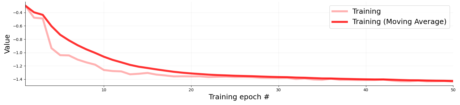
Figure 1 shows the loss defined in Equation 8 across the 50 training epochs (pink), together with its exponential moving average (red). The stabilization of the loss over epochs indicates that the training procedure has converged to a stable solution for the network parameters \((\hat{\phi}, \hat{\psi})\).10 As the loss has plateaued by 50 epochs, additional optimization is unlikely to yield substantial improvements.11 On average, updating the parameters of both neural networks during a single epoch took 122 seconds (95% interval: [99, 136] seconds). The hardware specifications are reported in Section 1 of the Supplementary Materials. A link to the learned network weights is provided in the Data Availability section below.
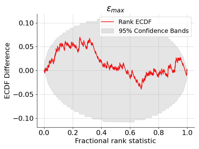
Once the parameters \((\hat{\phi}, \hat{\psi})\) have been learned, and before applying the model to empirical datasets to infer the values of \(\epsilon_{\max}\) most likely to have generated them, we use simulation-based calibration (SBC) to assess the self-consistency and precision of the learned approximate posterior, and recoverability tests to assess whether \(\epsilon_{\max}\) is identifiable from the learned summaries of the opinion distributions.
Specifically, we sampled \(200\) values of \(\epsilon_{max}\) from the corresponding prior and ran \(200\) instances of the bounded confidence model, generating \(200\) perturbed opinion distributions. We then treat each generated opinion distribution as if it were an empirical observation.
For each generated opinion distribution, we draw \(L = 3000\) realizations of the latent variable \(\boldsymbol{z}\) from a standard Gaussian distribution. These latent samples are then passed, together with the corresponding opinion distribution, through the trained normalizing flow with parameters \((\hat{\phi}, \hat{\psi})\) in the inverse direction (Equation 4, Algorithm 2). This procedure yields 200 estimated posterior distributions for \(\epsilon_{max}\), one for each opinion distribution, each consisting of 3000 posterior samples. The entire procedure is computationally inexpensive, taking an average of 5.35 seconds (95% interval: [5.29, 5.41] seconds).
Figure 2 reports the difference between the normalized ECDF of the rank statistics for the ground truth values of \(\epsilon_{max}\) within their corresponding posterior distributions and the cumulative distribution function of a normalized discrete uniform distribution over \(\{0,1,\dots,L\}\), with \(L=3000\) (see Section 3 and the Supplementary Materials for a detailed explanation of this statistic in the context of SBC).
As shown in Figure 2, the estimated posterior is well calibrated. The difference between the two cumulative distributions fluctuates around zero, and all deviations remain well within the confidence bands expected from finite-sample variability. This indicates that the posterior uncertainty and coverage can be considered reliable, with no evidence of systematic bias in the inferred posterior distributions (Betancourt 2020; Modrák 2025; Säilynoja et al. 2021; Talts et al. 2018).
Figure 3 assesses the identifiability of \(\epsilon_{\max}\) through a recoverability check (Betancourt 2020; van Ravenzwaaij & Oberauer 2009), which compares ground truth values of \(\epsilon_{\max}\) drawn from the prior with the posterior medians estimated from synthetic datasets generated under those values. The dotted diagonal line marks perfect recovery: if \(\epsilon_{\max}\) were fully identifiable, the posterior median obtained from each synthetic dataset would coincide with the ground-truth value that generated it, so that points would lie on the diagonal. The quantity \(r\) denotes the Pearson correlation coefficient between ground truth parameters and posterior median estimates. This correlation is high, indicating that larger ground truth values of \(\epsilon_{max}\) tend to be associated with larger posterior medians. However, the relationship is not linear: despite a correlation of \(r = 0.919\), there are substantial local deviations from exact one-to-one recovery across the parameter range.
More specifically, three distinct regimes can be identified. For ground truth values of \(\epsilon_{max}\) approximately between \(0.10\) and \(0.30\), the posterior median increases roughly linearly with the ground truth value, closely tracking the diagonal. In the context of the model, smaller values of \(\epsilon_{max}\) correspond to stronger homophily (i.e., greater narrow-mindedness) and give rise to multimodal opinion distributions that reflect fragmented societies (Hegselmann & Krause 2002; Renzini & Squazzoni 2026). The observed linear relationship in this range therefore indicates that the estimation algorithm is able to accurately discriminate between different degrees of narrow-mindedness in the population based on the resulting macroscopic opinion configurations.
For intermediate values between approximately \(0.30\) and \(0.40\), recovery quality deteriorates: posterior medians show a stronger tendency to fluctuate around \(0.35\) rather than tracking the diagonal. For ground truth values above approximately \(0.45\), posterior medians plateau around \(\approx 0.50\), irrespective of the generating value of \(\epsilon_{max}\). The transition region between \(0.40\) and \(0.45\) shows mixed behavior, with posterior medians alternating between approximately \(0.35\) and \(0.50\).
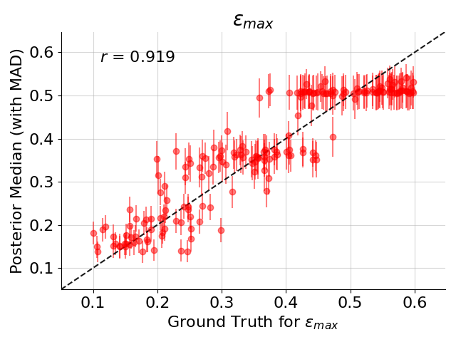
This cluster-like structure is consistent with the emergence of distinct macroscopic regimes for different values of \(\epsilon_{max}\) (Renzini & Squazzoni 2026). In particular, the clustering pattern reflects a transition between polarized states, characterized by bimodal opinion distributions, and consensus states, in which a single dominant opinion cluster emerges. This transition occurs around \(\epsilon_{max} \approx 0.45\), with both macroscopic states coexisting in the region \(\epsilon_{max} \in [0.40, 0.45]\).
Within these two regimes, the horizontal “streaks” of points indicate that distinct ground truth values of \(\epsilon_{max}\) yield very similar posterior medians. This pattern is suggestive of a loss of parameter identifiability when the estimation algorithm observes either a polarized or a consensus macroscopic opinion distribution. In other words, while the estimation algorithm can reliably distinguish whether the system exhibits polarization or consensus, it faces difficulties in discriminating between the specific parameter values within each regime that generated these macroscopic states, resulting in collapsed posterior median estimates around regime-typical values (\(\approx 0.35\) for polarization, \(\approx 0.50\) for consensus).
The extent to which this constitutes a substantive problem and warrants modifications to the model or the estimation pipeline must be assessed by jointly considering two factors. First, the recoverability test based on posterior medians is very stringent. In the two parameter clusters, posterior medians may differ from the ground truth values of \(\epsilon_{max}\), yet the true parameter values may still lie well within the central mass of the inferred posterior distributions (e.g., around the 35th or 60th percentile). From a Bayesian perspective, such deviations do not necessarily indicate poor inference, as ground truth values remain plausible under the posterior (Hines et al. 2014). Therefore, this test reveals whether our synthetic data contain sufficient information to pin down the generating parameter precisely at the posterior median. Strong agreement between the inferred posterior median and the ground truth values across the whole parameter space is desirable, but deviations may warrant further examination of the full posterior rather than reliance on point estimates alone.
Second, the practical relevance of this limited identifiability depends on both the research question and the empirical opinion distributions to which the model is applied (Preston et al. 2025). If empirical data predominantly reflect polarized systems, then making precise statements about the point estimate for the most frequent value12 of \(\epsilon_{max}\) that generated them is inherently difficult. This lack of resolution becomes problematic if the research question hinges on discriminating between such fine-grained differences in point estimates. By contrast, if empirical datasets span a broader range of macroscopic regimes, including fragmented, polarized, and consensus societies, and the inferential goal is to distinguish among these regimes rather than to pinpoint small parameter variations within a single regime, then the estimation algorithm retains sufficient discriminatory power to do so (Figure 3).
Inferring \(\epsilon_{max}\) from synthetic opinion distributions
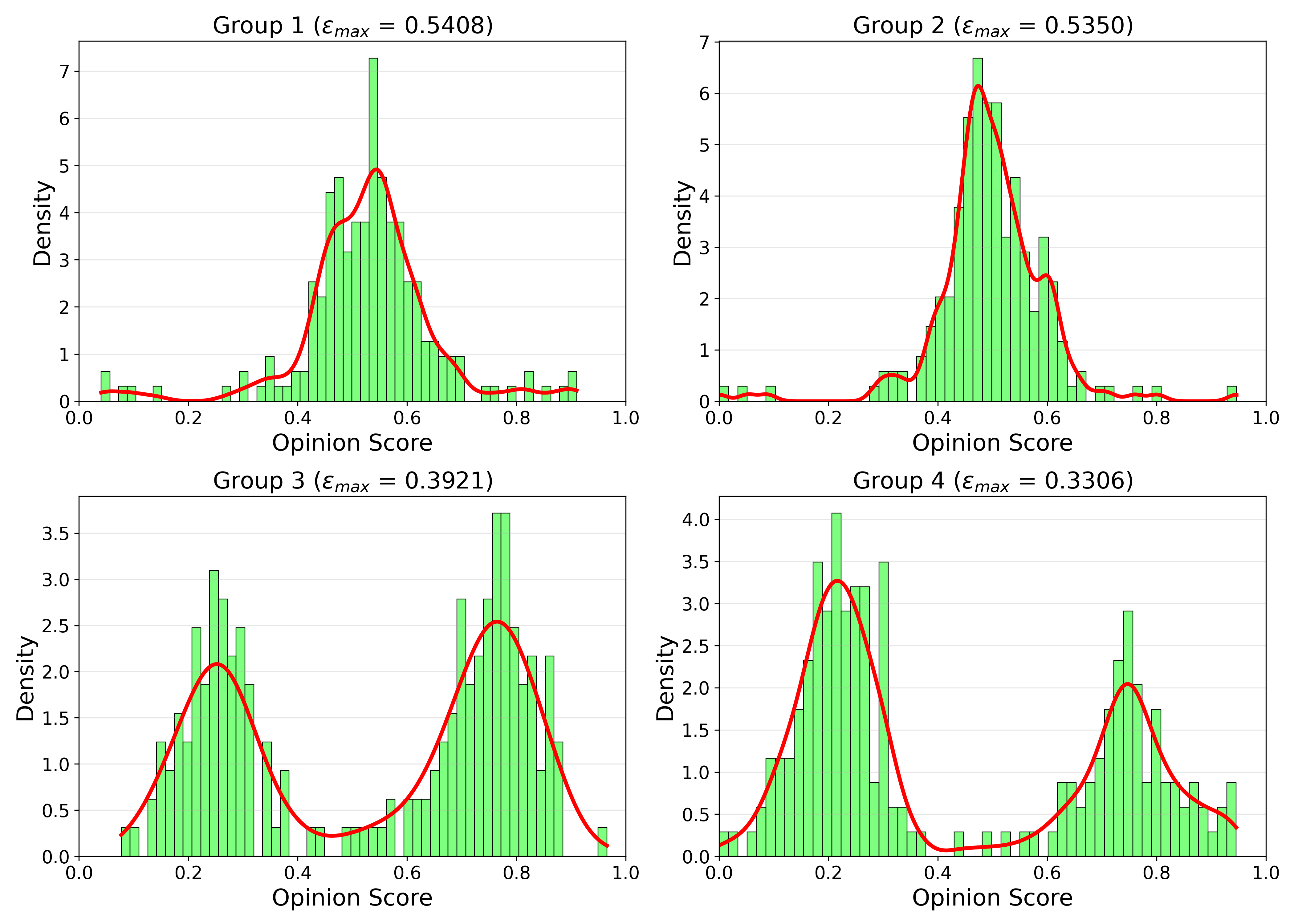
Figures 4 and 5 show, respectively, four empirical-like datasets and the corresponding posterior distributions for \(\epsilon_{max}\), each consisting of 3000 posterior samples, inferred using BayesFlow (Kühmichel et al. 2026) following Algorithm 2. Estimating the posterior distribution for each dataset took on average 0.0895 seconds (95% interval: [0.0729, 0.1061] seconds).
For illustrative purposes, the opinion distributions shown in Figure 4 are still synthetic, but we treat them as if they were sampled from four independent online communities discussing the same topic. Two of the datasets exhibit consensus, with most agents holding similar opinions, while the other two exhibit polarization, characterized by the emergence of bi-modal opinion clusters.
At first sight, the identifiability issues highlighted in Figure 3 appear less severe when examining the full posterior distributions rather than just point estimates (Olukan et al. 2026). As evident from Figure 5, while the ground truth \(\epsilon_{max}\) values do not fall exactly at the posterior median, they remain well-centered within the distributions, typically near the median percentiles.13 This pattern holds for both the communities that reached consensus (Groups 1 and 2) and those that split into two opposing, polarized camps (Groups 3 and 4).
However, parameter identifiability must also be assessed by examining the range of \(\epsilon_{max}\) values spanned by each posterior distribution (Hines et al. 2014; Olukan et al. 2026; Preston et al. 2025; Raue et al. 2009; Semochkina & Walsh 2025; Siekmann et al. 2012). Greater spread indicates that a greater number of distinct \(\epsilon_{max}\) values are capable of producing observationally similar opinion distributions under the model.
Whether higher variability constitutes a substantive problem depends on the implications of that variability for the underlying generative explanation. For the consensus groups (Groups 1 and 2), 91% of the posterior mass lies between \(0.40\) and \(0.60\). Substantively, this indicates that achieving consensus requires populations composed of open-minded agents with low levels of homophily. Importantly, the Beta distributions – and, consequently, the distributions of individual bounds of confidence \(\{\epsilon_i\}_{i=1}^{200}\) – generated by parameter values within this range are broadly similar. In these cases, a critical mass of agents effectively acts as bridges across different regions of the opinion space, remaining willing to assimilate opinions that differ substantially from their own. Thus, although the posterior spans multiple values of \(\epsilon_{max}\), these values are functionally equivalent and all support a common generative explanation: consensus emerges in populations that contain a variable but substantial proportion of open-minded agents characterized by weak homophily.
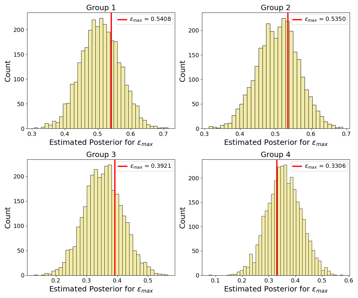
The polarized groups (Groups 3 and 4) present a potentially more concerning pattern. In both cases, a non-negligible fraction of the posterior mass (23% for Group 3 and 25% for Group 4) falls within the \([0.40, 0.60]\) interval. Parameter values in this range are more likely to produce consensus as the outcome. Consequently, conditional on a polarized opinion distribution, the estimation procedure assigns non-negligible posterior probability to values of \(\epsilon_{max}\) that are typically associated with consensus dynamics. This ambiguity may reflect genuine identifiability challenges.
Posterior contraction and retrodictive checks
Additional checks can be performed to assess the validity and performance of the estimation method, including posterior contraction and posterior retrodictive checks (Betancourt 2020). Posterior contraction, denoted by \(c\), addresses the question: how much information do the data provide beyond the prior? Specifically, it compares the variance of the posterior distribution of \(\epsilon_{max}\) to the variance of the prior distribution.
Posterior contraction is defined as:
| \[ c = 1 - \frac{\mathbb{V}_{\text{posterior}}[\epsilon_{\max}]}{\mathbb{V}_{\text{prior}}[\epsilon_{\max}]}\] | \[(11)\] |
Values of \(c\) close to zero indicate that the posterior closely resembles the prior distribution in terms of variance. Poor variance reduction, especially under a uniform prior spanning distinct behavioral regimes, is a further sign of non-identifiability. Conversely, values of \(c\) close to one indicate that the observations substantially reduce uncertainty about \(\epsilon_{max}\) beyond what is encoded in the prior model. However, a high \(c\) is not sufficient for identifiability, and should always be read together with recoverability checks and the shape of the posterior. Because \(c\) summarizes only the variance, a posterior with two nearby modes can still yield a high \(c\) while placing substantial probability mass on two distinct behavioral explanations, in which case fewer parameter values are consistent with the data but the parameter remains ambiguous between mechanisms.
In our application, we first drew \(3000\) samples from the prior distribution of \(\epsilon_{max}\) and computed the corresponding prior variance. We then computed posterior contraction for each of the four inferred posterior distributions shown in Figure 5, using this prior variance as denominator in Equation 11. The resulting contraction values are \(\{0.84, 0.84, 0.82, 0.81\}\), indicating substantial reduction in posterior uncertainty relative to the uniform prior. As noted above, however, posterior contraction should be interpreted jointly with the results shown in Figures 3 and 5, which provide complementary evidence for assessing whether \(\epsilon_{\max}\) is identifiable.
Posterior retrodictive checks proceed as follows. For each learned posterior distribution of \(\epsilon_{max}\) (Figure 5), we draw a fixed number of parameter samples (in our case, \(3000\)). Each sampled parameter value is then passed into the bounded confidence model to generate a corresponding simulated opinion distribution. This results in \(3000\) simulated datasets generated under each posterior, which are then compared to the original observed data (Figure 4). If the inferred posterior is well calibrated, the distributions generated from posterior samples should closely resemble the corresponding empirical opinion distributions (Betancourt 2020).
In our case, for simplicity, we compared the \(3000\) opinion distributions generated from posterior samples with the empirical data using the polarization metric introduced by Flache & Macy (2011). In Figure 6, we can see that posterior-generated simulations are able to reproduce this key macroscopic feature of the empirical opinion distributions. As expected, groups that exhibit polarization show higher values of this metric.
All results presented in this Section are potentially conditional on the architectures chosen for the summary neural network and the cINN, as well as on the dimensionality of the learned embedding \(\tilde{\boldsymbol{x}}\) and the model design parameters in \(\zeta\). The limitations highlighted in Figure 3 and the identifiability challenges illustrated in Figure 5 may therefore depend on these choices. For instance, if higher-order dependencies and correlations among agent opinions contain useful information to distinguish between consensus patterns when \(\epsilon_{max} \geq 0.45\), then using a SetTransformer may provide improved performance (see Sections 3.21 and 3.22). In the present analysis, we tried increasing the dimensionality of the embedding \(\tilde{\boldsymbol{x}}\) from 16 to 24, but this did not lead to improvements in this regard (see Figures S2 and S3 in the Supplementary Materials).
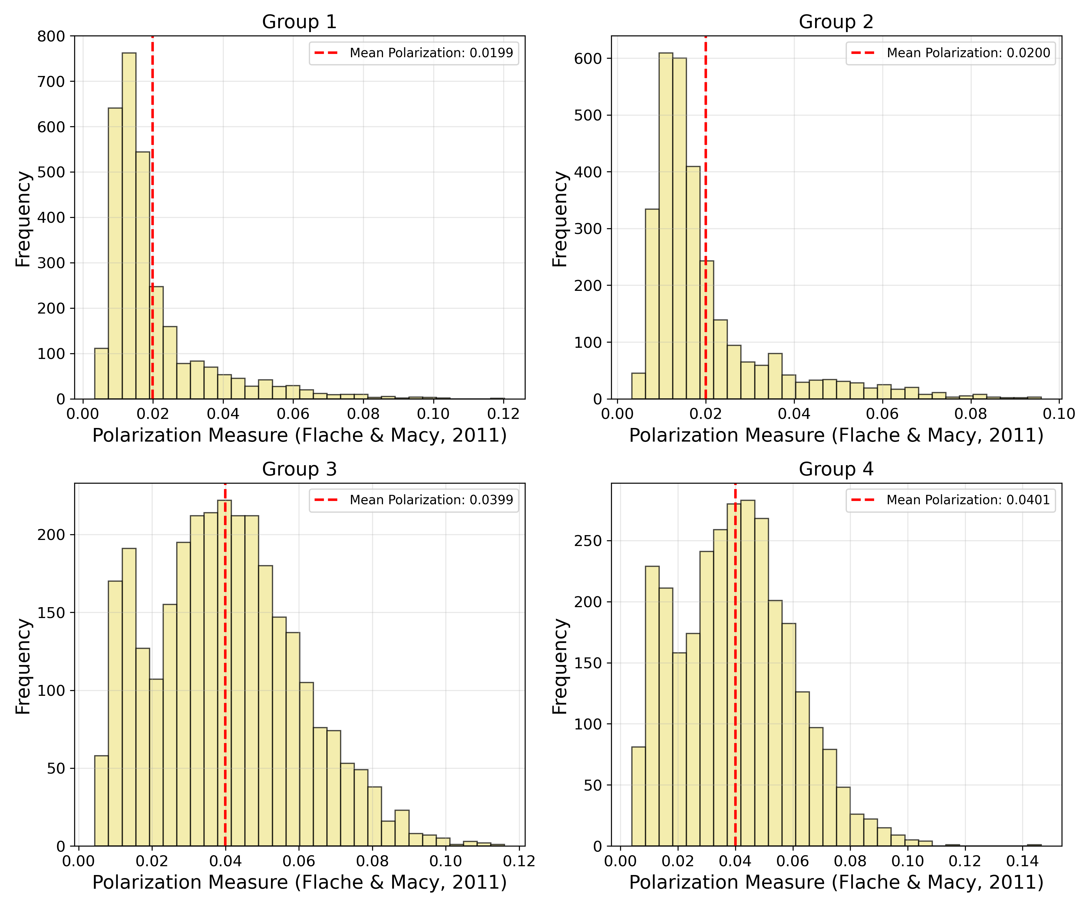
A SIR Model with Reporting Delays and Noisy Observations
Description
The second toy model is designed to explain the trajectory of an epidemic as the outcome of human-to-human transmission of an infectious disease (e.g., airborne transmission via droplets) within a population characterized by homogeneous mixing. Under this assumption, individuals have, on average, the same probability of encountering any other member of the population on a given day, implying comparable contact patterns across individuals and that encounters with infected individuals occur at a rate proportional to the overall disease prevalence in the population (Bansal et al. 2007; Radev et al. 2021).
We consider a population of \(A\) agents, indexed by \(i = 1, 2, \dots, A\). Each agent is characterized by a time-varying health status that can take one of three mutually exclusive values: susceptible, infected, or recovered. Susceptible agents are in good health but lack antibodies against the disease. Upon contact with an infected agent, a susceptible agent becomes infected with probability \(\lambda\), which captures the inherent infectiousness of the disease, net of any protective behaviors (Bansal et al. 2007). Higher values of \(\lambda\) correspond to a greater chance of infection upon contact. Once infected, agents remain ill until recovery occurs, which at each time step happens with probability \(\mu\). Upon recovery, agents transition to the recovered state and acquire immunity that prevents reinfection (Bansal et al. 2007).
We assume zero mortality, i.e., the disease is non-fatal, and permanent immunity following recovery. While these assumptions are stylized, a wide range of extensions that relax them, as well as the homogeneous mixing assumption, have been proposed in the literature (Bansal et al. 2007; Bostanci & Conrad 2025; Brauer 2008; Epstein et al. 2008; Eubank et al. 2008; Gozzi et al. 2025; Semochkina & Walsh 2025; Spooner et al. 2021).14
At time \(t_0\), a given number of "patient zero" agents is randomly assigned the infected status, so that the simulation starts with a total of \(I_{t_0}\) infected individuals. Under the homogeneous mixing assumption, each agent has an equal probability of encountering any other agent in the population. This allows for a description of the epidemic at the aggregate level, while still being directly grounded in the underlying individual-level movement rules and interaction patterns (Bicher & Popper 2013).
Let \(S_t\), \(I_t\), and \(R_t\) denote the total numbers of susceptible, infected, and recovered agents at time \(t\). The total number of infected agents evolves according to:
| \[ I_{t} = I_{t-1} - \mu I_{t-1} + I_{t-1 \rightarrow t}\] | \[(12)\] |
Time is modeled in discrete steps, where \(t-1\) and \(t\) represent two consecutive days. In Equation 12, \(I_{t-1 \rightarrow t}\) denotes the number of new cases that occur between day \(t-1\) and day \(t\), while \(\mu I_{t-1}\) represents the number of infected agents who transition to the recovered state during the same period, having developed immunity. The total number of new daily cases, \(I_{t-1 \rightarrow t}\), is determined as follows:
| \[ I_{t-1 \rightarrow t} = \lambda \frac{I_{t-1} S_{t-1}}{N}\] | \[(13)\] |
The total number of susceptible agents, \(S_t\), evolves according to the following:
| \[ S_{t} = S_{t-1} - I_{t-1 \rightarrow t}\] | \[(14)\] |
Finally, the total number of recovered agents, \(R_t\), evolves as:
| \[ R_{t} = R_{t-1} + \mu I_{t-1}\] | \[(15)\] |
From Equations 12–15 (Radev et al. 2021), it follows that as the number of infected agents increases, the number of susceptible agents decreases, while the number of recovered agents correspondingly increases. Equation 13 further implies that the peak in new daily cases occurs when there is both a sufficiently large number of infected agents circulating in the artificial population and a sufficiently large reservoir of immunologically naive agents who remain susceptible to infection.
We model an epidemic outbreak in a population of the same size as Germany (\(A = 83 \times 10^{6}\) agents; Radev et al. 2021). For each iteration, we first calculate the number of newly infected cases based on the previous state of the epidemic and the transmission probability \(\lambda\) (Equation 13), and then update the total numbers of susceptible, infected, and recovered agents accordingly. For each iteration, the model records two time series reporting the number of newly infected and newly recovered agents.15
In empirical settings, the actual number of individuals who become infected on a given day is rarely observed instantaneously (Radev et al. 2021). This is due to the incubation or symptom onset period, during which an individual is infected and capable of transmitting the disease while remaining asymptomatic or only mildly symptomatic. As a result, there is a delay of \(D\) days between the time an individual becomes infected – and thus can spread the disease if in contact with a susceptible agent – and the time at which the infection is likely to be detected by public health authorities.
Accordingly, we let the model evolve over a total period of \(50 + D\) days, but report as output \(\boldsymbol{x}\) only the two time series corresponding to days \(D\) through \(50 + D\). Hence, the reported time series have length 50, while the reporting delay \(D\), which determines the initial case detected by public health authorities, is treated as an unknown parameter to be estimated jointly with the transmission rate \(\lambda\), the recovery rate \(\mu\), and the initial number of infected agents \(I_{t_0}\) (Radev et al. 2021; Radev 2026). Fixing \((\lambda, \mu, I_{t_0})\) and varying \(D\) produces different reported epidemic trajectories, reflecting the effect of starting observations at different points given the same underlying epidemic dynamics (see Figure S4 in the Supplementary Materials).
Observed incidence data are subject to measurement error arising from misclassification, imperfections in diagnostic testing, and variations in testing capacity (e.g., fewer tests on certain days), resulting in noisy observations of both new infections and recoveries. To account for this, we specify an observation model in which each element of the observed time series is drawn from a negative binomial distribution (Radev et al. 2021). The mean of this distribution is given by the number of infected or recovered cases generated by the simulation, while the overdispersion parameter is fixed at 1.2, yielding a more irregular, "burstier" process than that implied by a Poisson distribution. The data entering the inference procedure therefore consist of these noisy observations. Importantly, observation noise affects only the reported data used for inference and does not feed back into the underlying epidemic dynamics governed by Equations 12–15.
Defining priors and describing the generative outcomes
For this model, we specify prior distributions over a four-dimensional parameter vector \(\theta = (\lambda, \mu, D, I_{t_0})\). For \(\lambda\), we assume a uniform distribution between 0.10 and 0.7, while the recovery probability \(\mu\) is drawn from a uniform distribution between 0.05 and 0.2. Following Radev et al. (2021), we assume that the reporting delay \(D\) is drawn from a lognormal distribution with mean \(\log(8)\) and standard deviation 0.2, while the initial number of infected agents \(I_{t_0}\) is drawn from a gamma distribution with shape 2 and scale 20. All prior draws are assumed to be mutually independent. Since both \(D\) and \(I_{t_0}\) must be integers but their prior distributions are continuous, we round the sampled values to the nearest integer after extraction (Radev et al. 2021).
We randomly assign the infected health status to a rounded number \(I_{t_0}\) of agents. Consequently, the initial number of susceptible individuals is \(A - I_{t_0}\), while the initial number of recovered individuals is assumed to be zero. Agents are then assumed to move and interact randomly with others in the artificial population, and the state of the population is updated using Equations 12–15, (Bicher & Popper 2013). The model output, \(\boldsymbol{x}\), consists of the noisy time series of incidence for newly infected and recovered cases.
Defining the summary neural network architecture
We begin estimating the model parameters \(\theta\) by considering only the time series of noisy new infected cases as data produced by the model (Radev 2026). Accordingly, our generated data \(\boldsymbol{x}\) is a sequence of 50 integers, \(\boldsymbol{x} = (x_{t_1}, x_{t_2}, \dots, x_{t_{50}})\). Our goal is to learn a lower-dimensional vector representation \(\tilde{\boldsymbol{x}}\) that captures the temporal dependencies among daily infected cases, as well as salient features of the epidemic dynamics such as peaks, troughs, growth rates and the presence of multiple waves. To this end, we employ a Gated Recurrent Unit (GRU; Chung et al. 2014; Radev 2026), a standard architecture for modeling sequential data that uses an adaptive gating mechanism to capture temporal dependencies (Lueckmann et al. 2017). We note that alternative standard recurrent architectures, such as LSTM networks (Table 1), could also have been employed (Radev et al. 2021). However, GRUs achieve comparable performance to LSTMs in many applications (Chung et al. 2014; Jozefowicz et al. 2015), while typically requiring fewer parameters and faster training.
The employed architecture is described in detail in the Supplementary Materials; here we provide an intuitive overview. A hidden state vector \(\mathbf{h}_0 = \mathbf{0}\in\mathbb{R}^{\kappa}\) is initialized and updated sequentially as the time series is processed (Radev 2026). At each time step \(t\in\{1,\ldots,50\}\), the GRU updates this hidden state through learnable gating mechanisms that regulate the flow of information between the current observation \(x_t\) and the previous hidden state. This allows to selectively retain or discard past information while incorporating new observations into the evolving representation. By recursively applying these updates across the sequence \(\boldsymbol{x}=(x_{t_{1}},x_{t_{2}},\dots,x_{t_{50}})\), the GRU learns features relevant for parameter inference from the temporal dynamics of the epidemic trajectory. For instance, it may capture long-range dependencies by associating early epidemic dynamics (e.g., at time step 10) with later behavior (e.g., at time step 40), while also identifying peaks, troughs, and multiple epidemic waves.
After processing all 50 time steps, the final hidden state \(\mathbf{h}_{50}\in\mathbb{R}^{\kappa}\) serves as a learned representation of the temporal information contained in the epidemic trajectory. This representation is subsequently compressed through a linear projection into the lower-dimensional summary vector \(\tilde{\boldsymbol{x}}\) (Lueckmann et al. 2017; Radev 2026). In our implementation, we choose \(\tilde{\boldsymbol{x}}\in\mathbb{R}^{8}\). The hyperparameters of the GRU architecture are reported in the Supplementary Materials.
Defining the cINN and the training schedule
The cINN architecture is identical to that used for the modified opinion dynamics model, and we adopt the same learning rate for the Adam optimizer. Training was performed for 100 epochs (Radev 2026), with each batch containing \(64\) simulated samples and each epoch comprising 120 batches. Therefore, each epoch processes \(64\times120=7680\) simulated trajectories, resulting in a total of \(64\times120\times100=768000\) simulated trajectories used to train the networks. The training schedule was adjusted according to the complexity of the inference problem. Since higher-dimensional parameter spaces often give rise to more complex posterior geometries and dependencies among parameters (Betancourt 2017), learning an accurate approximation of the posterior distribution may require additional simulated data and training iterations (Min et al. 2026; Radev et al. 2020).
Results
Training loss, diagnostic checks, and identifiability assessment
Figure 7 shows the loss function over the 100 training epochs (pink), together with its exponential moving average (red). The extension to 100 epochs was justified, as the loss continued to decrease beyond the first 50 epochs. The subsequent stabilization of the loss suggests that the training procedure converged to a stable set of network parameters \((\hat{\phi}, \hat{\psi})\), with further optimization unlikely to yield substantial improvements. On average, updating the parameters of both neural networks during a single epoch required 7.34 seconds (95% interval: [7.00, 9.00] seconds).
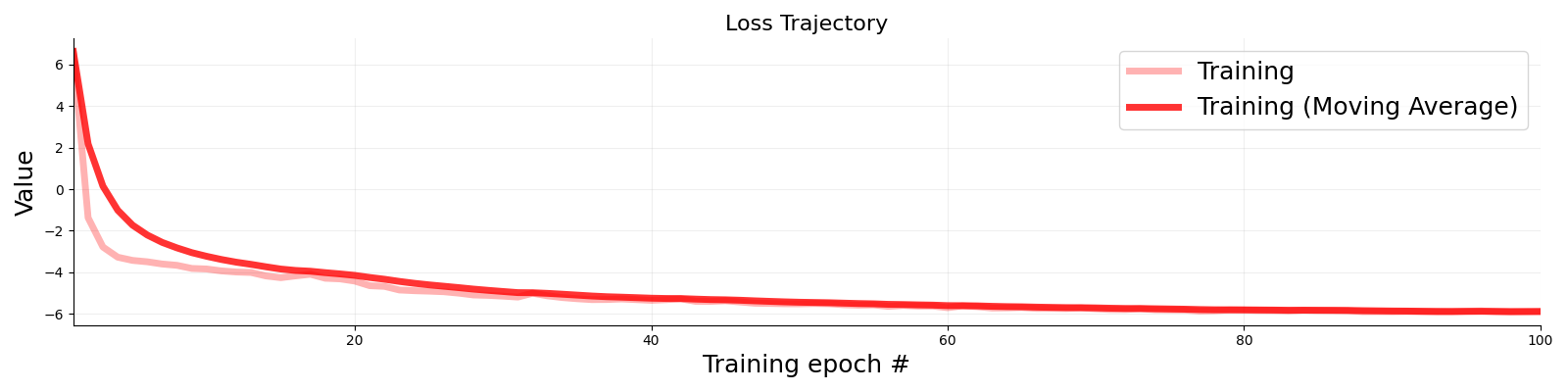
Figure 8 shows the ECDF difference plots for the marginal posterior distributions of the parameters in \(\theta = (\lambda, \mu, D, I_{t_0})\). The differences oscillate within the uncertainty bands around zero for all parameters, indicating that the uncertainty and coverage of the approximate posteriors are well calibrated (Betancourt 2020; Modrák 2025; Talts et al. 2018). The SBC test is constructed analogously to the case of the modified bounded confidence model. On average, the entire SBC procedure required 4.27 seconds (95% interval: [4.07, 4.47] seconds).
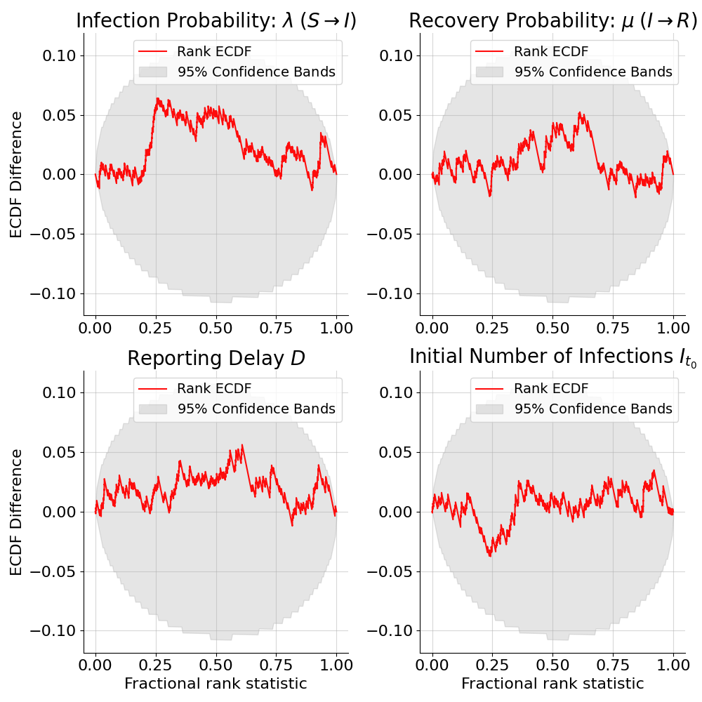
Figure 9 shows the relationship between the 200 ground truth parameter values also used in the SBC procedure and the medians of the corresponding approximate posterior distributions estimated from data simulated at those values. The infection probability \(\lambda\) is recovered almost exactly: for each ground truth value, the posterior median lies very close to the true value across the parameter space, producing a near-perfect linear relationship (\(r \approx 1\)). The initial number of infected individuals \(I_{t_0}\) is also recovered well, although with greater dispersion and lower precision than \(\lambda\).
We observe, however, that the recovery probability \(\mu\) and the reporting delay \(D\) appear to be weakly identified, as different ground truth values map, on average, to the same posterior medians across the parameter space (Radev 2026). We recall that the default recoverability diagnostic implemented in BayesFlow is very stringent. Passing this test – as in the case of \(\lambda\) – provides strong evidence that the inference procedure can accurately recover the corresponding model parameter. Failing the test does not necessarily indicate non-identifiability tout court; rather, it calls for a closer inspection of the posterior distributions at selected points in the parameter space. Indeed, the ground truth value may not coincide with the posterior median but can still be found near regions of high posterior density (Figures 3 and 5). Moreover, the posterior probability mass may shift in accordance with the true parameter value, such that as the ground truth increases, the mass moves toward higher values. In this sense, the model may still be able to capture qualitatively distinct regimes (Figures 3 and 5).
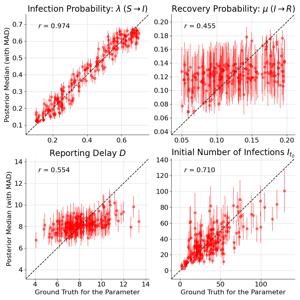
Figures 10 and 11 show the inferred posterior distributions for selected ground truth values spanning the parameter ranges of \(\mu\) and \(D\), respectively. In contrast to the behavior observed for \(\epsilon_{max}\) in Figure 5, many ground truth values now lie in the tails of the corresponding approximate posteriors.
Moreover, the inferred posteriors are largely invariant across the parameter space, exhibiting only weak sensitivity to changes in the underlying ground truth values. For instance, approximately halving \(\mu\) from \(0.19\) to \(0.10\) results in nearly indistinguishable posterior distributions (bottom row of Figure 10), while a similar lack of sensitivity is observed when approximately doubling \(D\) (top row of Figure 11). This pattern is further corroborated by posterior contraction diagnostics. For \(\mu\), with the exception of the top-left case (\(c = 0.74\)), contraction values are very small in the remaining cases (\(\{0.04, 0.13, 0.08\}\)), indicating little to no variance reduction relative to the prior. The situation is similar for \(D\), for which posterior contraction values are small (\(\{0.007, 0.17, 0.16, 0.26\}\)).
Taken together, these findings suggest that the estimation procedure is unlikely to reliably identify \(\mu\) and \(D\) when relying solely on time series of daily new infected cases (Radev 2026).
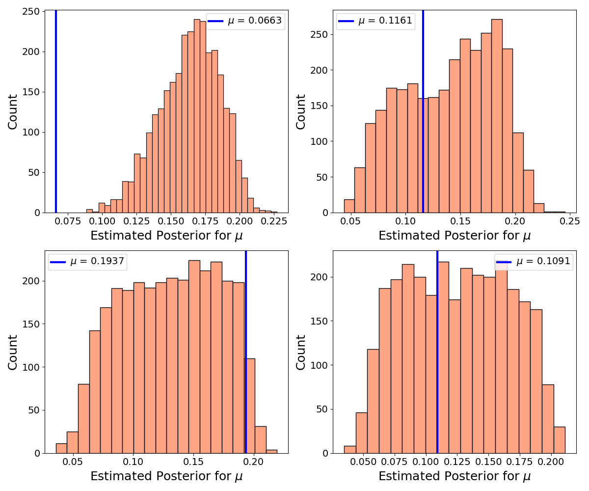
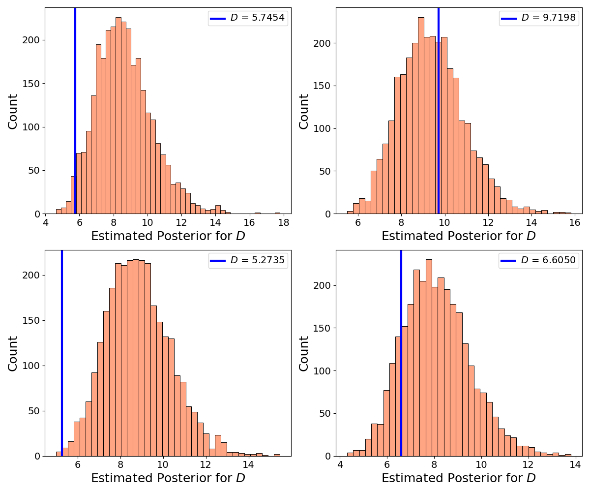
We investigate whether the identifiability issues can be mitigated by enriching the information provided to the estimation algorithm (Daly et al. 2018; Preston et al. 2025). Specifically, we train the inference pipeline on a multivariate time series comprising both daily new infected and daily new recovered cases. Including information on recoveries may provide the estimation algorithm with additional information to better identify the recovery probability \(\mu\) and the reporting delay \(D\) (Porthiyas et al. 2024; Preston et al. 2025).
We note that, in a Bayesian framework, identifiability is inherently tied to the choice of prior distributions (Gelman 2014; Neath & Samaniego 1997; Rannala 2002; Semochkina & Walsh 2025). For example, in the first toy model, suppose that the prior for \(\epsilon_{max}\) were a uniform distribution on the interval \([0.10, 0.25]\). If Figure 3 were restricted to this range, no apparent identifiability issues would emerge, as posterior medians within this interval are approximately linearly related to their corresponding ground truth values.
However, we deliberately refrain from modifying the prior distributions, as we argue that such a practice is warranted only when additional information becomes available from sources external to the model (Betancourt 2020; Semochkina & Walsh 2025), such as previously unavailable expert knowledge or new empirical estimates. Altering priors solely to render a model identifiable risks inducing overfitting, overstating inferential precision, or even excluding potentially valid explanations. Accordingly, we treat the chosen priors as the most plausible ex ante specifications and focus on assessing what can – and cannot – be learned from the data under these assumptions.
Introducing the time series of recovered cases
We adopt an architecture that first preprocesses the multivariate time series using a convolutional neural network (CNN) and then passes the extracted features to a GRU-based summary network followed by a linear projection layer (BayesFlow 2026; Zhang & Mikelsons 2023). Specifically, a convolutional layer operates on the \(2\times50\) matrix generated by the SIR simulator, extracting local cross-series features from the joint temporal dynamics of infected and recovered incidence. These features are then fed into the same GRU architecture as before. To provide greater representational capacity for modeling multivariate temporal dependencies, the resulting summary vector \(\tilde{\boldsymbol{x}}\) is chosen to be 16-dimensional (BayesFlow 2026). The corresponding hyperparameters are reported in the Supplementary Materials.
Using an identical training schedule as the univariate case, the increased architectural complexity resulted in an average epoch training time of 13.46 seconds (95% interval: [12.0, 18.0] seconds). Training proceeded stably, and the loss converged smoothly within 100 epochs (Figure 12).
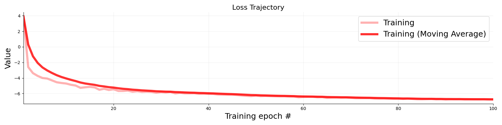
Turning to parameter identifiability, Figure 13 shows that recovery remains excellent for the transmission probability \(\lambda\) and generally improves for the initial number of infected individuals \(I_{t_{0}}\). As expected, incorporating the time series of newly recovered cases substantially improves the identifiability of the recovery probability \(\mu\), as the algorithm can now leverage additional observations to disentangle competing parameter configurations. The relationship between ground truth values and posterior medians is now markedly more linear than in Figure 9, with the Pearson correlation increasing from \(r = 0.455\) to \(r = 0.789\). By contrast, the reporting delay \(D\) remains poorly identified, with no improvement in recoverability despite the richer data (Radev 2026).
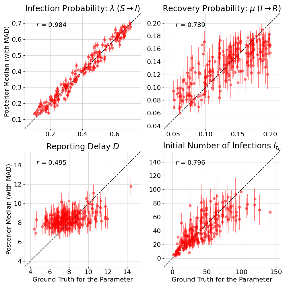
Because BayesFlow approximates the full multivariate posterior distribution \(p(\theta_1, \theta_2, \dots, \theta_D \mid \boldsymbol{x})\), we can inspect both marginal posterior distributions and their pairwise dependencies, providing additional information to understand why this may be the case. Figure 14 shows the pairwise dependency plot for a representative evaluation dataset simulated with ground-truth parameters \(\lambda = 0.439\), \(\mu = 0.149\), \(D = 9\), and \(I_{t_0} = 20\). The diagonal panels display the marginal posterior distributions (dark green) alongside the respective priors (lime), the upper triangular panels show pairwise scatter plots of posterior draws, and the lower triangular panels show the corresponding two-dimensional kernel density contours.
We can see that the posterior for \(D\) is updated only weakly compared to the prior, whereas the posteriors for the other parameters contract substantially. This is confirmed by the contraction statistics \(c(\lambda) = 0.97\), \(c(\mu) = 0.66\), \(c(D) = 0.26\), and \(c(I_{t_{0}}) = 0.85\). \(D\) is largely uncorrelated with the rates \(\lambda\) and \(\mu\), which directly govern the evolution and peaks of daily incident infections and recoveries (Equations 12–15). By contrast, \(D\) is negatively related to \(I_{t_{0}}\), suggesting a compensatory relationship whereby a shorter reporting delay combined with more initial cases produces observed trajectories similar to those from a longer delay combined with fewer initial cases. During early growth, \(I_{t_{0}}\) and \(D\) jointly set the level and starting point of the observed epidemic trajectory. Taken together, these results suggest that the two incidence series carry limited information about \(D\) separately from \(I_{t_{0}}\). In other words, the data allow \(I_{t_{0}}\) to absorb, or “mute”, much of the variation that would otherwise be attributed to \(D\).
Figure 15 further reinforces this interpretation through posterior retrodictive checks on the full time series of incident infections and recoveries across four synthetic datasets. The fit is excellent for all datasets, suggesting that accurate reproduction of the observed epidemic trajectories does not require \(D\) to be precisely identified. This confirms that aggregate time series alone carry insufficient signal to identify \(D\), and that additional data – such as line lists with precise diagnostic timestamps – would be necessary to do so.
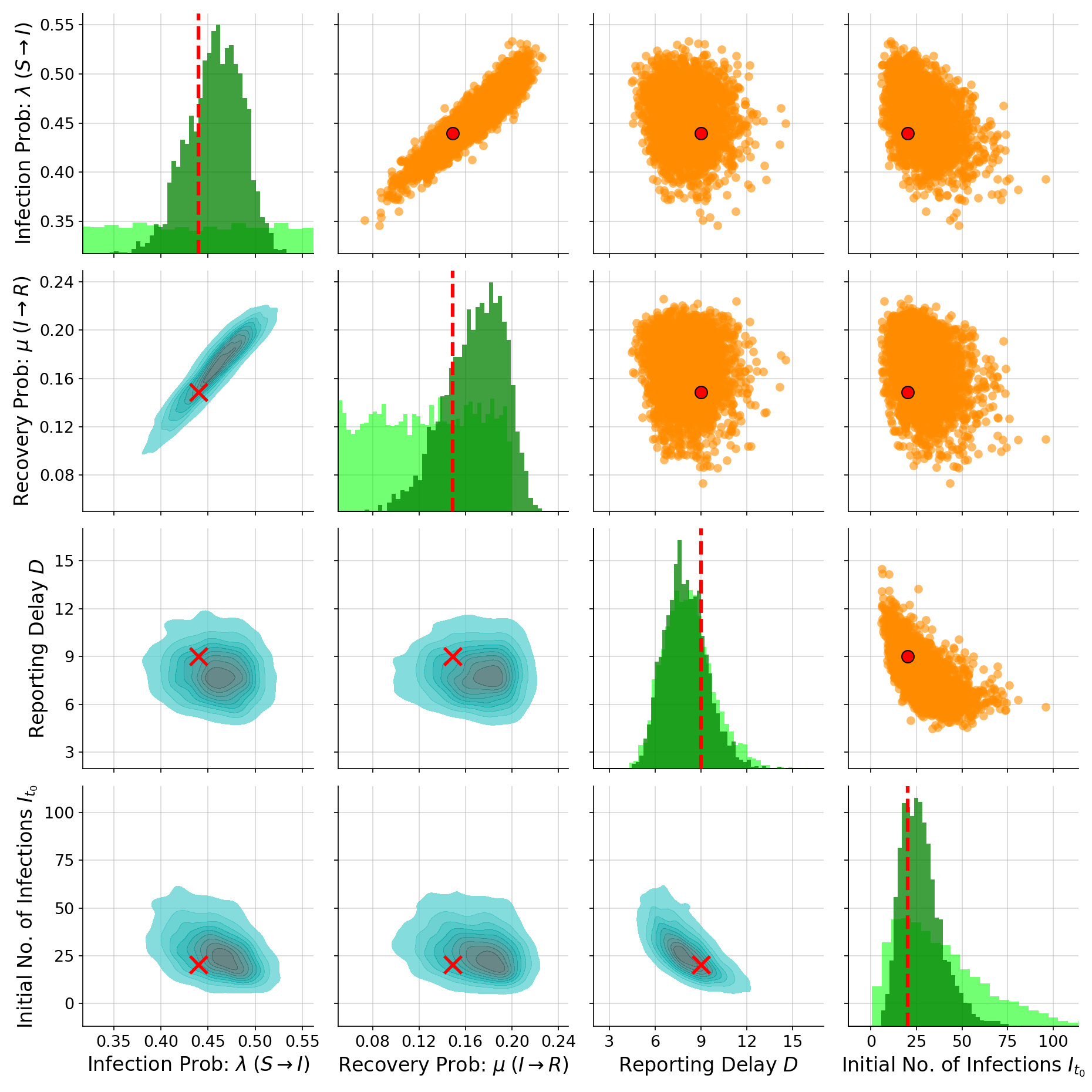
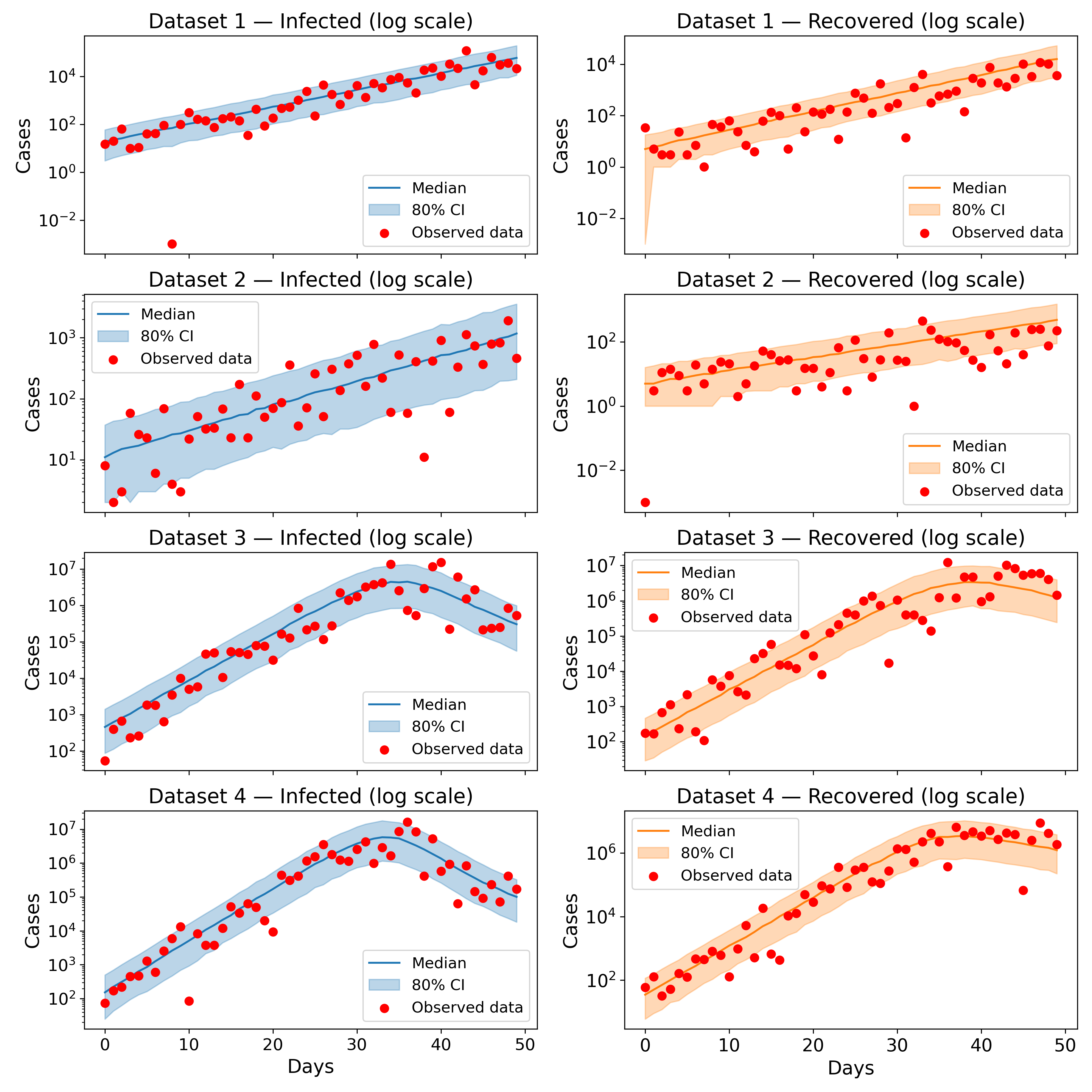
Dealing with the non-identifiability of parameter \(D\)
So far, we have established that identifiability is jointly determined by the structure of the model and the information content of the available data (Preston et al. 2025). Suppose now that the only information available for training the inference procedure consists of the two incidence time series of daily infected and recovered cases. Under this constraint, what strategies can be adopted to address the non-identifiability of \(D\)?
As already anticipated, one possible response is to revise the prior distributions (Neath & Samaniego 1997; Rannala 2002; Semochkina & Walsh 2025), ideally when new information becomes available. For example, newly published evidence or expert assessments may suggest that the symptom onset period is likely shorter than one week, thereby justifying a more informative prior for the reporting delay \(D\).
An alternative option is to reparameterize the model (Preston et al. 2025). For example, consider a model of the form:
| \[\text{output} = \theta_{1} e^{\left(\theta_{2} \cdot \text{input} + \theta_{3}\right)}\] | \[(16)\] |
In this specification, \(\theta_{1}\) and \(\theta_{3}\) are not separately identifiable, since they enter the model only through their product,
| \[\theta_{1} e^{\theta_{3}} e^{\left(\theta_{2} \cdot \text{input}\right)}\] | \[(17)\] |
However, the composite parameter given by their product, \(\theta_{1} e^{\theta_{3}}\), is identifiable (Collin et al. 2021; Preston et al. 2025).16 Analogously, in the present setting we may not be able to identify \(I_{t_{0}}\) and \(D\) separately, yet it may still be possible to identify composite functions of these parameters, such as their product or ratio.
A final option is to revise the generative mechanism itself, either by enriching it with additional processes that render \(D\) identifiable, or by simplifying the model in a way that better aligns its parameters with the available observable data.
Crucially, regardless of the chosen strategy, it is essential to transparently report the fact that parameter recoverability and identification failed under earlier model specifications and to document how subsequent modeling decisions were informed by this limitation. Concealing such failures would deprive the modeling community of valuable information and undermine scientific credibility. Selectively presenting only well-performing model specifications while omitting reasonable but unsuccessful alternatives would be akin to practices such as p-hacking or HARKing, and should be avoided.
It is important to note that augmenting the data to improve parameter recoverability and identifiability may come at the cost of degraded uncertainty quantification or the introduction of systematic biases for some parameters, as revealed by SBC (Figure 16, in particular for \(D\)). Several strategies could be pursued to mitigate this issue. These include modifying the observation model to increase stochasticity, training deeper or more expressive cINN architectures, extending training through additional epochs, or modifying the architecture of the summary network.
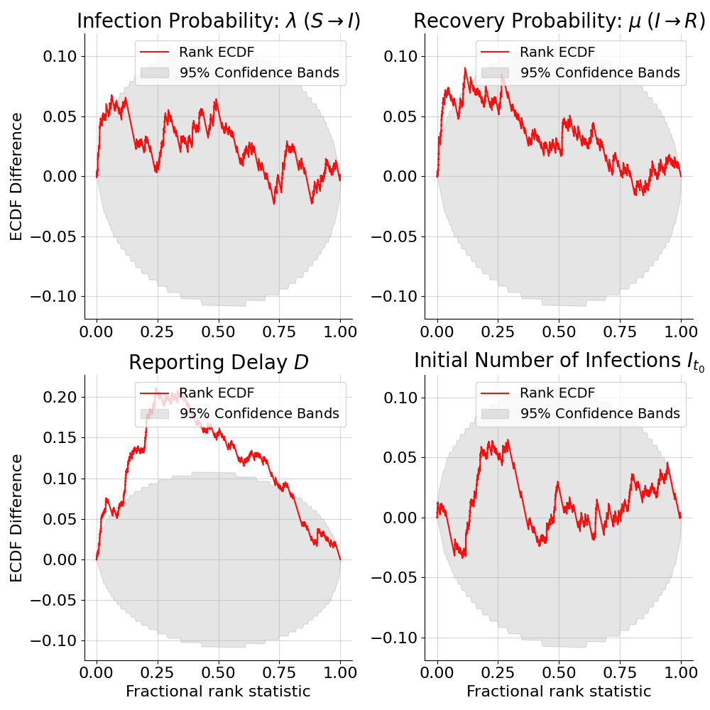
Discussion and Conclusions
Identifying the range of parameter combinations of a given model that are consistent with empirical observables is of paramount importance for agent-based modelers. This can expose important identifiability issues that might render inferences drawn from data about the hypothesized generative mechanisms ambiguous at best or entirely invalid. When such issues go unnoticed, they can lead to substantial prediction errors and, ultimately, to misleading downstream policy implications and recommendations (Alarid-Escudero et al. 2018; Preston et al. 2025; Raue et al. 2009; Semochkina & Walsh 2025; Villaverde 2019).
Bayesian statistics is a natural framework for addressing this challenge, as the target estimand is a distribution of parameter values – the posterior distribution – which researchers can inspect to detect identifiability issues and assess their severity through characteristics such as its width, shape, and the dependencies among parameters (Olukan et al. 2026). Moreover, the Bayesian framework supports principled diagnostic procedures to assess whether the inferred posterior distributions provide reliable parameter estimates (Betancourt 2020).
Here, we have presented a powerful algorithm based on normalizing flows for estimating posterior distributions of model parameters given data, originally introduced by Radev et al. (2020) and implemented in the Python package BayesFlow (Kühmichel et al. 2026; Radev et al. 2023). We illustrated its use through a step-by-step application to two toy models: (i) a bounded confidence model with heterogeneous bounds of confidence, and (ii) a SIR epidemiological model with reporting delays and noisy observations of the daily incidence of infected and recovered cases. Our modifications to these well-known models were designed to create settings in which the identifiability of certain parameters depended on the data available to the estimation algorithm.
Importantly, all the identifiability assessments through parameter recoverability checks (Betancourt 2020), as well as the posterior inferences themselves and other diagnostic checks such as SBC (Talts et al. 2018), were carried out systematically and almost instantaneously. This is because BayesFlow performs amortized inference (Radev et al. 2020): unlike methods such as ABC-SMC (Olukan et al. 2026), once the networks have been trained, they can be applied to any new dataset, empirical or synthetic, without re-running the estimation. This allowed us to perform a thorough and detailed diagnostic analysis, contextualize identifiability issues in light of the substantive aims of the modeler, and discuss a set of possible strategies to address them.
We summarize these strategies below as a list of questions, covering the possible actions we have implemented or discussed in this manuscript (Preston et al. 2025). Such actions are not mutually exclusive: several can be combined, and doing so may resolve non-identifiability more effectively than any single change alone, though this is not guaranteed, as this depends on the specific application.
- Has new information from external sources, rather than the data at hand, become available that would support a more informative prior?
- Is there existing information in the available data that the estimation procedure is not yet exploiting? For example, we found that incorporating the time series of newly recovered cases, in addition to infections alone, substantially improved the identifiability of the recovery rate \(\mu\) in the SIR model with reporting delays.
- Is the summary network architecture capturing all the relevant structure in the data? Which features of the data are particularly informative about the underlying generative process? Would a more expressive architecture (e.g., an attention-based or deeper network) help distinguish between competing parameter configurations?
- Can the model be reparametrized so that inference targets an identifiable combination of the original parameters, rather than each parameter individually (e.g., a ratio or product)?
- Can the generative mechanism itself be revised, either by enriching it with additional processes that render the parameter identifiable by better connecting it to the available data, or by simplifying it, including possibly dropping the parameter altogether, if it is not essential to the modeler’s substantive aims or to the model’s predictive capacity?
There are some limitations to the present work. First, the two toy models considered in this paper are computationally inexpensive to simulate, and the upfront training procedure could become substantially more demanding for computationally intensive ABMs with more complex dynamics or larger parameter spaces. In such settings, offline learning provides a possible alternative to online training: a fixed number of simulations is generated in advance according to the available computational budget and subsequently reused during training (Radev et al. 2020; Shiono 2021).
A more ambitious avenue for future research would be to combine BayesFlow with emulator- or surrogate-based approaches (Lamperti et al. 2018; Robertson et al. 2025). Rather than repeatedly evaluating the original ABM during training, a machine-learning model could be trained to approximate the mapping from model parameters to simulation outputs. The BayesFlow inference pipeline could operate on this computationally inexpensive emulator instead of directly on the simulator, reducing the overall training cost. Developing such an integrated framework would require jointly accounting for the approximation error introduced by the emulator and the training objectives of the summary and inference networks.
Second, because BayesFlow is amortized, it can be readily applied to multiple datasets, either observed or synthetic, once training is complete. However, reliable generalization requires that the training simulations adequately cover the range of observations likely to be encountered at inference time. For complex models, generating sufficiently diverse training data may be challenging, and the quality of the learned estimator inevitably depends on the choice of prior distributions from which the parameters used to generate the training simulations are sampled (Min et al. 2026).
Third, in some applications modelers may be primarily interested in matching domain-specific summary statistics identified through stakeholder input or established in the literature as relevant benchmarks. In such cases, the learned embeddings produced by the summary network may be less directly interpretable or comparable to these predefined quantities. Nevertheless, BayesFlow can also operate with hand-crafted summary statistics (Kühmichel et al. 2026; Olischläger 2026). Moreover, although we have focused on the quality of posterior inference and identifiability assessment, we have also shown that the inferred posteriors can support predictive analyses (Figures 6 and 15). When a modeler’s primary objective is to reproduce a single observed dataset, simpler optimization-based approaches may achieve comparable predictive performance at substantially lower computational cost (Figure S5 in the Supplementary Materials).
Finally, BayesFlow is not the only framework that integrates normalizing flows into Bayesian parameter estimation. For a broader perspective on this class of methods, we refer readers to Dyer et al. (2024) and Min et al. (2026). While BayesFlow specifically employs conditional invertible neural networks (cINNs), other conditional normalizing flow architectures can also be used, including RealNVP (Dinh et al. 2016), Masked Autoregressive Flows (Dyer et al. 2022; Papamakarios et al. 2017), and Neural Spline Flows (Durkan et al. 2017). Other neural-network-based simulation-based inference pipelines are also available (e.g., Dignum et al. 2025), although these do not rely on normalizing flows.
Concerning future developments, in this work we applied the inference procedure to multiple datasets independently and assessed the resulting posteriors separately. A natural extension would be to integrate hierarchical priors to account for the variation of model parameters between observed groups, in a manner akin to mixed-effects or multi-level models. An important step in this direction within the BayesFlow framework has been proposed by Habermann et al. (2025).
In conclusion, we expect parameter estimation to become an increasingly important part of ABM research in the era of big data and AI (Renzini et al. 2023). Fast and systematic uncertainty quantification, aimed at diagnosing potential identifiability issues, is therefore essential, because such issues can propagate to theoretical inferences, predictions, and policy recommendations. Despite its limitations, we hope that this study encourages researchers to consider BayesFlow as a practical tool for this purpose, and thereby fosters cumulative methodological development and more systematic applications of simulation-based inference in ABM research.
Supplementary Materials
The Supplementary Materials file can be found here: https://github.com/ceco51/Bayesian-Normalizing-Flows/blob/main/SM_JASSS_FR.pdf
Model Documentation
The Python code required to replicate the estimation and diagnostic checks for both toy models are available here: https://github.com/ceco51/Bayesian-Normalizing-Flows/blob/main/Bounded%20Confidence%20Model/BC-BF.ipynb (modified bounded confidence model), and here: https://github.com/ceco51/Bayesian-Normalizing-Flows/blob/main/SIR%20Model/PaperSIR.ipynb (SIR model).
The code is organized into two separate Jupyter (IPython) notebooks.
Data Availability
Here (https://github.com/ceco51/Bayesian-Normalizing-Flows/tree/main/Bounded%20Confidence%20Model), we provide the .csv files for the four empirical-like opinion distribution datasets shown in Figure 4, the corresponding recovered posteriors displayed in Figure 5, and the values of the loss function over epochs. In addition, we share the learned weights \((\hat{\phi}, \hat{\psi})\) for both the cINN and Deep Set networks in the modified bounded confidence model case as .pkl files here: https://github.com/ceco51/Bayesian-Normalizing-Flows/blob/main/Bounded%20Confidence%20Model/trained_weights_raw.pkl.
For the first estimated SIR model (using only the time series of newly infected cases), the learned weights \((\hat{\phi}, \hat{\psi})\) for both the cINN and the GRU networks are available as .pkl files here: https://github.com/ceco51/Bayesian-Normalizing-Flows/blob/main/SIR%20Model/trained_weights_raw_first_model.pkl. The corresponding loss over epochs is available as a .csv file here: https://github.com/ceco51/Bayesian-Normalizing-Flows/blob/main/SIR%20Model/training_loss_first_model.csv.
For the second SIR model (using the two time series), the learned weights \((\hat{\phi}, \hat{\psi})\) for both the cINN and the CNN+GRU networks are available as .pkl files here: https://github.com/ceco51/Bayesian-Normalizing-Flows/blob/main/SIR%20Model/trained_weights_raw_second_model.pkl. The corresponding loss over epochs is available as a .csv file here: https://github.com/ceco51/Bayesian-Normalizing-Flows/blob/main/SIR%20Model/training_loss_second_model.csv.
Notes
- Despite recent advances in inverse generative social science (iGSS; Epstein 2023), which aim to infer the generative mechanism itself from data, we assume here that \(g(\cdot)\) is specified a priori by the researcher (Poole & Raftery 2000; Radev et al. 2020).↩︎
- Each \(\theta \in \Theta\) may be a \(D\)-dimensional vector of integers, real numbers, or a mixture of both. Examples of such behavioral parameters include traders’ sensitivity to specific market signals (e.g., Gao et al. 2024; Renzini & Epstein 2026) and network formation preferences (e.g., Renzini et al. 2024; Renzini 2025).↩︎
- See Toni et al. (2009) for details on the calculation of the importance weights.↩︎
- Without loss of generality, we assume that the vectors are continuous, or may contain discrete elements that can be treated as continuous and re-discretized if necessary.↩︎
- Under online learning, the parameters of both the summary network and the cINN are updated iteratively using mini-batches of size \(M\) consisting of simulation-parameter-latent variable tuples over \(E\) epochs. This approach allows the networks to continuously incorporate newly simulated data, supports progressive refinement of the posterior approximation, and reduces overfitting relative to standard offline learning strategies, which rely on a fixed training dataset and a held-out validation set for parameter updates (Radev et al. 2021).↩︎
- For instance, the default configuration of a Gated Recurrent Unit (GRU) architecture reflects established recommendations and practices from the GRU literature.↩︎
- Accordingly, the observed opinion for agent \(i\) is given by \(\hat{o}_{i}^{T} = o_{i}^{T} + u_{i}\), where \(u_{i} \sim \mathcal{N}(0, 0.07^{2})\). The latent opinion \(o_{i}^{T}\) results from a sequence of 50 endogenous interactions with other agents, governed by the individual-specific bound of confidence \(\epsilon_{i}\). For simplicity, we assume that reporting noise is additive, independent across individuals, and of known variance. In the second toy model, parts of the observation model are estimated as well. Here, we emphasize that this specification is mainly illustrative: alternative assumptions (e.g., correlated reporting errors or heteroskedastic noise) could affect the estimation pipeline.↩︎
- Histograms, cumulative distribution functions, moments (e.g., mean, variance, skewness, kurtosis), indices derived from such moments (e.g., the Jarque-Bera statistic or polarization measures), positional statistics (e.g., median, percentiles, minimum, maximum), the mode, as well as moments and positional statistics of pairwise or groupwise differences (provided that groups are not defined by positional neighbors in the set, i.e., those immediately preceding or following a given element), are invariant under permutations of a given distribution.↩︎
- See https://www.scibits.blog/posts/deepsets/ for further details and an accessible tutorial.↩︎
- Note that \((\hat{\phi}, \hat{\psi})\) are not guaranteed to correspond to the global optimum of the objective function and may instead represent a local minimum or stationary point.↩︎
- Notably, the loss appears to stabilize around epoch 35, suggesting that a shorter training schedule may have achieved comparable performance in this setting.↩︎
- Assuming approximate normality, so that the posterior median coincides with its mode.↩︎
- Recomputing Figure 3 using other point estimates such as the mean or mode instead of the median produces similar results. As shown in Figure 5, the posteriors are approximately normal, so the mean, mode, and median largely coincide.↩︎
- We emphasize that the primary purpose of the two toy models considered here is to illustrate how
BayesFlowcan be used to conduct parameter inference and assess identifiability in agent-based models. Accordingly, simplicity of exposition and sufficient generality to ensure accessibility to a broad audience are prioritized over realism. Bounded-confidence and SIR models are well established in the literature and provide a suitable testbed for our methodological objectives.↩︎ - Note that we focus on incidence, i.e., the number of marginally new infected and recovered agents, rather than on prevalence, i.e., the stock or cumulative number of individuals in the \(I\) and \(R\) compartments.↩︎
- That is, the data may only allow us to infer that \(\theta_{1} e^{\theta_{3}} = 4\), while infinitely many combinations of \(\theta_{1}\) and \(e^{\theta_{3}}\) yield this same value when multiplied together.↩︎
References
ALARID-ESCUDERO, F., MacLehose, R. F., Peralta, Y., Kuntz, K. M., & Enns, E. A. (2018). Nonidentifiability in model calibration and implications for medical decision making. Medical Decision Making, 38(7). [doi:10.1177/0272989x18792283]
ANSTETT-COLLIN, F., Denis-Vidal, L., & Millérioux, G. (2020). A priori identifiability: An overview on definitions and approaches. Annual Reviews in Control, 50, 139–149. [doi:10.1016/j.arcontrol.2020.10.006]
BANKS, D. L., & Hooten, M. B. (2021). Statistical challenges in agent-based modeling. The American Statistician, 75(3), 235–242. [doi:10.1080/00031305.2021.1900914]
BANSAL, S., Grenfell, B. T., & Ancel Meyers, L. (2007). When individual behaviour matters: Homogeneous and network models in epidemiology. Journal of the Royal Society Interface, 19(4), 879–891. [doi:10.1098/rsif.2007.1100]
BAYESFLOW. (2026). Documentation for BayesFlow network architectures. Available at: https://bayesflow.org/v2.0.12/api/bayesflow.networks.html.
BEAUMONT, M. A. (2019). Approximate Bayesian Computation. Annual Review of Statistics and Its Application, 6, 379–403. [doi:10.1146/annurev-statistics-030718-105212]
BELLOTTI, E., Bianchi, F., Renzini, F., Nengnong, C. B., van Eijk, A. M., Kessler, A., Sarkar, R., Carlton, J. M., & Albert, S. (2026). Negative ties offset complex contagion effecton malaria preventive measure adoption in a hard-to-reach population. SocArXiv preprint. Available at: https://osf.io/preprints/socarxiv/nxqwy_v1. [doi:10.31235/osf.io/nxqwy_v1]
BERGER, J. O., Liseo, B., & Wolpert, R. L. (1999). Integrated likelihood methods for eliminating nuisance parameters. Statistical Science, 14(1), 1–22. [doi:10.1214/ss/1009211804]
BERNARDO, C., Altafini, C., Proskurnikov, A., & Vasca, F. (2024). Bounded confidence opinion dynamics: A survey. Automatica, 159, 111302. [doi:10.1016/j.automatica.2023.111302]
BETANCOURT, M. (2017). A conceptual introduction to Hamiltonian Monte Carlo. arXiv preprint. Available at: https://arxiv.org/abs/1701.02434.
BETANCOURT, M. (2020). Towards a principled Bayesian workflow. Available at: https://betanalpha.github.io/assets/case_studies/principled_bayesian_workflow.html.
BETZ, G. (2022). Natural-Language multi-Agent simulations of argumentative opinion dynamics. Journal of Artificial Societies and Social Simulation, 25(1), 2. [doi:10.18564/jasss.4725]
BICHER, M., & Popper, N. (2013). Agent-based derivation of the SIR-differential equations. Proceedings of the 2013 8th EUROSIM Congress on Modelling and Simulation. [doi:10.1109/eurosim.2013.62]
BORRILL, P., & Tesfatsion, L. (2011). Agent-based modeling: The right mathematics for the social sciences? In J. B. Davis & D. W. Hands (Eds.), Elgar Companion to Recent Economic Methodology. Cheltenham: Edward Elgar. [doi:10.4337/9780857938077.00018]
BOSTANCI, I., & Conrad, T. (2025). Integrating agent-based and compartmental models for infectious disease modeling: A novel hybrid approach. Journal of Artificial Societies and Social Simulation, 28(1), 5. [doi:10.18564/jasss.5567]
BRAUER, F. (2008). Compartmental models in epidemiology. In F. BRAUER, P. Driessche, & J. Wu (Eds.), Mathematical Epidemiology (Vol. 1, pp. 19–79). Berlin Heidelberg: Springer. [doi:10.1007/978-3-540-78911-6_2]
BREHMER, J. (2021). Simulation-based inference in particle physics. Nature Reviews Physics, 3, 305. [doi:10.1038/s42254-021-00305-6]
CALVEZ, B., & Hutzler, G. (2005). Automatic tuning of agent-based models using genetic algorithms. In International Workshop on Multi-Agent Systems and Agent-Based Simulation (Vol. 1, pp. 41–57). Berlin Heidelberg: Springer. [doi:10.1007/11734680_4]
CARRELLA, E. (2020). Estimating agent-based models. Available at: https://carrknight.github.io/abm/2020/09/22/estimation.html.
CARRELLA, E. (2021). No free lunch when estimating simulation parameters. Journal of Artificial Societies and Social Simulation, 24(2), 7. [doi:10.18564/jasss.4572]
CHAPRON, P., Leclaire, M., Scriban, A., Masse, D., Reuillon, R., Fallot, A., & Delay, E. (2026). Fallow land simulations to fight against soil degradation: Engaging stakeholders with model exploration. Journal of Artificial Societies and Social Simulation, 29(1), 3. [doi:10.18564/jasss.5816]
CHUNG, J., Gulcehre, C., Cho, K. H., & Bengio, Y. (2014). Empirical evaluation of gated recurrent neural networks on sequence modeling. arXiv preprint. Available at: https://arxiv.org/pdf/1412.3555.
COLLIN, F. D., Durif, G., Raynal, L., Lombaert, E., Gautier, M., Vitalis, R., Marin, J. M., & Estoup, A. (2021). Extending approximate Bayesian computation with supervised machine learning to infer demographic history from genetic polymorphisms using DIYABC Random Forest. Molecular Ecology Resources, 21(8), 2598–2613. [doi:10.1111/1755-0998.13413]
COLLINS, A., Koehler, M., & Lynch, C. (2024). Methods that support the validation of agent-Based models: An overview and discussion. Journal of Artificial Societies and Social Simulation, 27(1), 11. [doi:10.18564/jasss.5258]
COWAN, G. (2013). Introduction to likelihoods. Likelihood Workshop CERN, 21–23, 2013. Available at: https://indico.cern.ch/event/218693/contributions/1520325/attachments/353588/492541/cowan_cern_likelihood.pdf.
CRANMER, K., Brehmer, J., & Louppe, G. (2020). The frontier of simulation-based inference. Proceedings of the National Academy of Sciences, 117(48), 30055–30062. [doi:10.1073/pnas.1912789117]
CSILLÉRY, K., Blum, M. G. B., Gaggiotti, O. E., & François, O. (2010). Approximate Bayesian Computation (ABC) in practice. Trends in Ecology & Evolution, 25(7), 410–418. [doi:10.1016/j.tree.2010.04.001]
DALY, A. C., Gavaghan, D., Cooper, J., & Tavener, S. (2018). Inference-based assessment of parameter identifiability in nonlinear biological models. Journal of the Royal Society Interface, 15(144), 20180318. [doi:10.1098/rsif.2018.0318]
DEISTLER, M., Boelts, J., Steinbach, P., Moss, G., Moreau, T., Gloeckler, M., Rodrigues, P. L. C., Linhart, J., Lappalainen, J. K., Kurt Miller, B., Gonçalves, P. J., Lueckmann, J. M., Schröder, C., & Macke, J. H. (2025). Simulation-based inference: A practical guide. arXiv preprint. Available at: https://arxiv.org/abs/2508.12939. [doi:10.21105/joss.07754]
DIGGLE, P. J., & Gratton, R. J. (1984). Monte Carlo methods of inference for implicit statistical models. Journal of the Royal Statistical Society: Series B (Methodological), 46(2), 193–212. [doi:10.1111/j.2517-6161.1984.tb01290.x]
DIGNUM, E., Boterman, W., Flache, A., & Lees, M. (2025). Empirically estimating an agent-based model of school choice on household-level register data. Journal of Artificial Societies and Social Simulation, 28(4), 8. [doi:10.18564/jasss.5798]
DINH, L., Sohl-Dickstein, J., & Bengio, S. (2016). Density estimation using Real NVP. arXiv preprint. Available at: https://arxiv.org/abs/1605.08803.
DOSOVITSKIY, A., Beyer, L., Kolesnikov, A., Weissenborn, D., Zhai, X., Unterthiner, T., Dehghani, M., Minderer, M., Heigold, G., Gelly, S., Uszkoreit, J., & Houlsby, N. (2020). An image is worth 16x16 words: Transformers for image recognition at scale. arXiv preprint. Available at: https://arxiv.org/abs/2010.11929.
DURKAN, C., Bekasov, A., Murray, I., & Papamakarios, G. (2017). Neural spline flows. arXiv preprint. Available at: https://arxiv.org/abs/1906.04032.
DYER, J., Cannon, P., Farmer, J. D., & Schmon, S. M. (2022). Calibrating agent-based models to microdata with graph neural networks. ICML Workshop on AI for Agent-based Modelling.
DYER, J., Cannon, P., Farmer, J. D., & Schmon, S. M. (2024). Black-box Bayesian inference for agent-based models. Journal of Economic Dynamics and Control, 161, 104827. [doi:10.1016/j.jedc.2024.104827]
EDMONDS, B., Le Page, C., Bithell, M., Chattoe-Brown, E., Grimm, V., Meyer, R., Montañola-Sales, C., Ormerod, P., Root, H., & Squazzoni, F. (2019). Different modelling purposes. Journal of Artificial Societies and Social Simulation, 22(3), 6. [doi:10.18564/jasss.3993]
EPSTEIN, J. M. (2006). Generative Social Science: Studies in Agent-Based Computational Modeling. Princeton, NJ: Princeton University Press. [doi:10.23943/princeton/9780691158884.003.0003]
EPSTEIN, J. M. (2008). Why model? Journal of Artificial Societies and Social Simulation, 11(4), 12.
EPSTEIN, J. M. (2023). Inverse generative social science: Backward to the future. Journal of Artificial Societies and Social Simulation, 26(2), 9. [doi:10.18564/jasss.5083]
EPSTEIN, J. M., Parker, J., Cummings, D., & Hammond, R. A. (2008). Coupled contagion dynamics of fear and disease: Mathematical and computational explorations. PLoS One, 3(12), e3955. [doi:10.1371/journal.pone.0003955]
EUBANK, S., Guclu, H., Anil Kumar, V. S., Marathe, M. V., Srinivasan, A., Toroczkai, Z., & Wang, N. (2008). Modelling disease outbreaks in realistic urban social networks. Nature, 429, 180–184. [doi:10.1038/nature02541]
FLACHE, A., & Macy, M. (2011). Small worlds and cultural polarization. Journal of Mathematical Sociology, 35(1–3), 146–176. [doi:10.1080/0022250x.2010.532261]
FLACHE, A., Mäs, M., Feliciani, T., Chattoe-Brown, E., Deffuant, G., Huet, S., & Lorenz, J. (2017). Models of social influence: Towards the next frontiers. Journal of Artificial Societies and Social Simulation, 20(4), 2. [doi:10.18564/jasss.3521]
FRANKE, R. (2009). Applying the method of simulated moments to estimate a small agent-based asset pricing model. Journal of Empirical Finance, 16(5), 804–815. [doi:10.1016/j.jempfin.2009.06.006]
GABRY, J., Simpson, D., Vehtari, A., Betancourt, M., & Gelman, A. (2019). Visualization in Bayesian workflow. Journal of the Royal Statistical Society Series A: Statistics in Society, 182(2), 389–402. [doi:10.1111/rssa.12378]
GAO, K., Vytelingum, P., Weston, S., Luk, W., & Guo, C. (2024). High-Frequency financial market simulation and flash crash scenarios analysis: An agent-based modelling approach. Journal of Artificial Societies and Social Simulation, 27(2), 8. [doi:10.18564/jasss.5403]
GELMAN, A. (2014). How to think about “identifiability” in Bayesian inference? Available at: https://statmodeling.stat.columbia.edu/2014/02/12/think-identifiability-bayesian-inference/.
GELMAN, A., Carlin, J. B., Stern, H. S., Dunson, D. B., Vehtari, A., & Rubin, D. B. (2013). Bayesian Data Analysis. Chapman & Hall/CRC. [doi:10.1201/b16018]
GOZZI, N., Chinazzi, M., Davis, J. T., Gioannini, C., Rossi, L., Ajelli, M., Perra, N., & Vespignani, A. (2025). Epydemix: An open-source Python package for epidemic modeling with integrated approximate Bayesian calibration. PLoS Computational Biology, 21(11), e1013735. [doi:10.1371/journal.pcbi.1013735]
GRIMM, V., Revilla, E., Berger, U., Jeltsch, F., Mooij, W. M., Railsback, S. F., Thulke, H. H., Weiner, J., Wiegand, T., & DeAngelis, D. L. (2005). Pattern-oriented modeling of agent-based complex systems: Lessons from ecology. Science, 310(5750), 987–991. [doi:10.1126/science.1116681]
GUNARATNE, C., Hatna, E., Epstein, J. M., & Garibay, I. (2023). Generating mixed patterns of residential segregation: An evolutionary approach. Journal of Artificial Societies and Social Simulation, 26(2), 7. [doi:10.18564/jasss.5081]
GUTMANN, M. U., & Corander, J. (2016). Bayesian optimization for likelihood-free inference of simulator-Based statistical models. Journal of Machine Learning Research, 17, 1–47.
HABERMANN, D., Schmitt, M., Kühmichel, L., Bulling, A., Radev, S. T., & Bürkner, P. C. (2025). Amortized Bayesian multilevel models. arXiv preprint. Available at: https://arxiv.org/abs/2408.13230. [doi:10.1214/25-ba1570]
HAZELBAG, C. M., Dushoff, J., Dominic, E. M., Mthombothi, Z. E., & Delva, W. (2020). Calibration of individual-based models to epidemiological data: A systematic review. PLoS Computational Biology, 16(5), e1007893. [doi:10.1371/journal.pcbi.1007893]
HEGSELMANN, R., & Krause, U. (2002). Opinion dynamics and bounded confidence: Models, analysis and simulation. Journal of Artificial Societies and Social Simulation, 5(3), 2.
HINES, K. E., Middendorf, T. R., & Aldrich, R. W. (2014). Determination of parameter identifiability in nonlinear biophysical models: A Bayesian approach. Journal of General Physiology, 143(3), 401–416. [doi:10.1085/jgp.201311116]
HOOTEN, M., Wikle, C., & Schwob, M. (2020). Statistical implementations of agent-based demographic models. International Statistical Review, 88(2), 441–461. [doi:10.1111/insr.12399]
HUNTER, E., & Duggan, J. (2025). A multi-method study evaluating the inference of compartmental model parameters from a generative agent-based model. Infectious Disease Modelling, 11(1), 218–240. [doi:10.1016/j.idm.2025.10.002]
JOZEFOWICZ, R., Zaremba, W., & Sutskever, I. (2015). An empirical exploration of recurrent network architectures. Proceedings of the 32nd International Conference on Machine Learning, Lille, France, 2015.
KINGMA, D. P., & Welling, M. (2013). Auto-encoding variational Bayes. arXiv preprint. Available at: https://arxiv.org/abs/1312.6114.
KIPF, T. N., & Welling, M. (2017). Semi-supervised classification with graph convolutional networks. arXiv preprint. Available at: https://arxiv.org/abs/1609.02907.
KOBYZEV, I., Prince, S. J. D., & Brubaker, M. A. (2020). Normalizing flows: An introduction and review of current methods. arXiv preprint. Available at: https://arxiv.org/abs/1908.09257.
KOTTHOFF, F., & Hamacher, T. (2022). Calibrating agent-based models of innovation diffusion with gradients. Journal of Artificial Societies and Social Simulation, 25(3), 4. [doi:10.18564/jasss.4861]
KÜHMICHEL, L., Huang, J. M., Pratz, V., Arruda, J., Olischläger, H., Habermann, D., Kucharsky, S., Elsemüller, L., Mishra, A., Bracher, N., Jedhoff, S., Schmitt, M., Bürkner, P. C., & Radev, S. T. (2026). BayesFlow 2.0: Multi-backend amortized Bayesian inference in Python. arXiv preprint. Available at: https://www.arxiv.org/abs/2602.07098. [doi:10.21105/joss.05702]
LAM, N. N., Docherty, P. D., & Murray, R. (2022). Practical identifiability of parametrised models: A review of benefits and limitations of various approaches. Mathematics and Computers in Simulation, 199, 202–216. [doi:10.1016/j.matcom.2022.03.020]
LAMPERTI, F., Roventini, A., & Sani, A. (2018). Agent-based model calibration using machine learning surrogates. Journal of Economic Dynamics and Control, 90, 366–389. [doi:10.1016/j.jedc.2018.03.011]
LEA, C., Vidal, R., Reiter, A., & Hager, G. D. (2016). Temporal convolutional networks: A unified approach to action segmentation. arXiv preprint. Available at: https://arxiv.org/abs/1608.08242. [doi:10.1007/978-3-319-49409-8_7]
LECUN, Y., Bottou, L., Bengio, Y., & Haffner, P. (1998). Gradient-based learning applied to document recognition. Proceedings of the IEEE, 86, 2278–2324. [doi:10.1109/5.726791]
LEE, J., LEE, Y., Kim, J., Kosiorek, A. R., Choi, S., & Teh, Y. W. (2019). Set Transformer: A framework for attention-based permutation-Invariant neural networks. arXiv preprint. Available at: https://arxiv.org/abs/1810.00825.
LI, Y., Tarlow, D., Brockschmidt, M., & Zemel, R. (2017). Gated graph sequence neural networks. arXiv preprint. Available at: https://arxiv.org/abs/1511.05493.
LIN, H., & Jegelka, S. (2018). ResNet with one-neuron hidden layers is a universal approximator. arXiv preprint. Available at: https://arxiv.org/abs/1806.10909.
LIN, M., Wen, K., Zhu, X., Zhao, H., & Sun, X. (2023). Graph autoencoder with preserving node attribute similarity. Entropy, 25(4), 567. [doi:10.3390/e25040567]
LORENZ, J. (2010). Heterogeneous bounds of confidence: Meet, discuss and find consensus! Complexity, 15(4), 43–52. [doi:10.1002/cplx.20295]
LORENZ, J. (2012). Continuous opinion dynamics under bounded confidence. Available at: https://ccl.northwestern.edu/netlogo/models/community/bc.
LOUPPE, G. (2026). An introduction to simulation-based inference. Available at: https://glouppe.github.io/info8004-advanced-machine-learning/pdf/glouppe-sbi.pdf.
LUECKMANN, J. M., Goncalves, P. J., Bassetto, G., Öcal, K., Nonnenmacher, M., & Macke, J. H. (2017). Flexible statistical inference for mechanistic models of neural dynamics. arXiv preprint. Available at: https://arxiv.org/abs/1711.01861.
LUX, T., & Zwinkels, R. C. J. (2018). Empirical validation of agent-Based models. In C. Hommes & B. LeBaron (Eds.), Handbook of Computational Economics (Vol. 4, pp. 437–488). Amsterdam: Elsevier. [doi:10.1016/bs.hescom.2018.02.003]
MANZO, G. (2022). Agent-Based Models and Causal Inference. Hoboken, NJ: John Wiley Sons.
MCCULLOCH, J., Ge, J., Ward, J. A., Heppenstall, A., Polhill, J. G., & Malleson, N. (2022). Calibrating agent-based models using uncertainty quantification methods. Journal of Artificial Societies and Social Simulation, 25(2), 1. [doi:10.18564/jasss.4791]
MCPHERSON, M., Smith-Lovin, L., & Cook, J. M. (2001). Birds of a feather: Homophily in social networks. Annual Review of Sociology, 27, 415–444. [doi:10.1146/annurev.soc.27.1.415]
MICHELS, A. C., Kang, J. Y., & Wang, S. (2022). Particle swarm optimization for calibrating agent-based models: A case study on a spatially-explicit model of Influenza transmission. Journal of Artificial Societies and Social Simulation, 25(2), 8. [doi:10.18564/jasss.4796]
MIN, J., Ning, Y., Pope, N. S., Baumdicker, F., & Kern, A. D. (2026). Neural posterior estimation for population genetics. Genetics, 233(3), iyag107. [doi:10.1093/genetics/iyag107]
MODRÁK, M. (2025). SBC rank visualizations. Available at: https://hyunjimoon.github.io/SBC/articles/rank_visualizations.html.
NEATH, A. A., & Samaniego, F. J. (1997). On the efficacy of Bayesian inference for nonidentifiable models. The American Statistician, 51(3), 225–232. [doi:10.1080/00031305.1997.10473967]
OLISCHLÄGER, H. (2026). Rapid iteration with point estimation – Lotka-Volterra dynamics. BayesFlow documentation. Available at: https://bayesflow.org/v2.0.13/_examples/Lotka_Volterra_Point_Estimation.html.
OLUKAN, D., Ward, J., Malleson, N., & Ge, J. (2026). Heterogeneity in agent-based models. Journal of Artificial Societies and Social Simulation, 29(2), 5. [doi:10.18564/jasss.5872]
PAPAMAKARIOS, G., Nalisnick, E., Rezende, D. J., Mohamed, S., & Lakshminarayanan, B. (2021). Normalizing flows for probabilistic modeling and inference. Journal of Machine Learning Research, 22, 1–64.
PAPAMAKARIOS, G., Pavlakou, T., & Murray, I. (2017). Masked autoregressive flow for density estimation. arXiv preprint. Available at: https://arxiv.org/abs/1705.07057.
PAYETTE, N. (2024). The curse of possibilities. In C. Elsenbroich & H. Verhagen (Eds.), Advances in Social Simulation (Vol. 3, pp. 601–608). Berlin Heidelberg: Springer.
PETRONE, S., Rousseau, J., & Scricciolo, C. (2014). Bayes and emprical Bayes: Do they merge? Biometrika, 101, 285–302. [doi:10.1093/biomet/ast067]
PLATT, D. (2020). A comparison of economic agent-based model calibration methods. Journal of Economic Dynamics and Control, 113, 103859. [doi:10.1016/j.jedc.2020.103859]
PLATT, D., & Gebbie, T. (2018). Can agent-based models probe market microstructure? Physica A: Statistical Mechanics and Its Applications, 503, 1092–1106. [doi:10.1016/j.physa.2018.08.055]
POOLE, D., & Raftery, A. E. (2000). Inference for deterministic simulation models: The Bayesian melding approach. Journal of the American Statistical Association, 95(452), 1244–1255. [doi:10.1080/01621459.2000.10474324]
PORTHIYAS, J., Nussey, D., Beauchemin, C. A. A., Warren, D. C., Quirouette, C., & Wilkie, K. P. (2024). Practical parameter identifiability and handling of censored data with Bayesian inference in mathematical tumour models. npj Systems Biology and Applications, 10, 89. [doi:10.1038/s41540-024-00409-6]
PRESTON, S. P., Wilkinson, R. D., Clayton, R. H., Chappell, M. J., & Mirams, G. R. (2025). Think before you fit: Parameter identifiability, sensitivity and uncertainty in systems biology models. Current Opinion in Systems Biology, 42, 100563. [doi:10.1016/j.coisb.2025.100563]
RADEV, S. T. (2026). Posterior estimation for SIR-like models. BayesFlow documentation. Available at: https://bayesflow.org/v2.0.12/_examples/SIR_Posterior_Estimation.html.
RADEV, S. T., Graw, F., Chen, S., Mutters, N. T., Eichel, V. M., Bärnighausen, T., & Köthe, U. (2021). OutbreakFlow: Model-based Bayesian inference of disease outbreak dynamics with invertible neural networks and its application to the COVID-19 pandemics in Germany. PLoS Computational Biology, 17(10), e1009472. [doi:10.1371/journal.pcbi.1009472]
RADEV, S. T., Mertens, U. K., Voss, A., Ardizzone, L., & Köthe, U. (2020). BayesFlow: Learning complex stochastic models with invertible neural networks. arXiv preprint. Available at: https://arxiv.org/abs/2003.06281. [doi:10.1109/tnnls.2020.3042395]
RADEV, S. T., Schmitt, M., Schumacher, L., Elsemüller, L., Pratz, V., Schälte, Y., Köthe, U., & Bürkner, P. C. (2023). BayesFlow: Amortized Bayesian workflows with neural networks. Journal of Open Source Software, 8(89), 5702. [doi:10.21105/joss.05702]
RANNALA, B. (2002). Identifiability of parameters in MCMC Bayesian inference of phylogeny. Systematic Biology, 51(5), 754–760. [doi:10.1080/10635150290102429]
RAUE, A., Kreutz, C., Maiwald, T., Bachmann, J., Schilling, M., Klingmüller, U., & Timme, J. (2009). Structural and practical identifiability analysisn of partially observed dynamical models by exploiting the profile likelihood. Bioinformatics, 25(15), 1923–1929. [doi:10.1093/bioinformatics/btp358]
RAYNAL, L., Marin, J. M., Pudlo, P., Ribatet, M., Robert, C. P., & Estoup, A. (2019). ABC random forests for Bayesian parameter inference. Bioinformatics, 35(10), 1720–1728. [doi:10.1093/bioinformatics/bty867]
RENZINI, F. (2025). Network formation dynamics in asymmetric coordination games. Rationality & Society, 37(3), 356–394. [doi:10.1177/10434631241309265]
RENZINI, F., Bianchi, F., & Squazzoni, F. (2024). Status, cognitive overload, and incomplete information in advice-seeking networks: An agent-based model. Social Networks, 76, 150–159. [doi:10.1016/j.socnet.2023.09.001]
RENZINI, F., Debernardi, C., Bianchi, F., Cremonini, M., & Squazzoni, F. (2023). The new frontiers of social simulation in the data science era: An introduction to the proceedings. In F. Squazzoni (Ed.), Advances in Social Simulation (Vol. 3, pp. 1-10). Cham: Springer Nature Switzerland. [doi:10.1007/978-3-031-34920-1_1]
RENZINI, F., & Epstein, J. M. (2026). Fear and financial contagion: Modeling animal spirits in asset markets. SocArXiv preprint. Available at: https://osf.io/preprints/socarxiv/rqxhm_v1. [doi:10.31235/osf.io/rqxhm_v1]
RENZINI, F., & Squazzoni, F. (2026). Using computer simulations to study social dynamics. In A. L. Nichols & J. E. Edlund (Eds.), The Cambridge Handbook of Research Methods and Statistics for the Social and Behavioral Sciences (Vol. 3, pp. 684-708). Cambridge: Cambridge University Press. ISBN: 9781009000819.
REUILLON, R., Leclaire, M., & Rey-Coyrehourcq, S. (2015). OpenMOLE, a workflow engine specifically tailored for the distributed exploration of simulation models. Future Generation Computer Systems, 29(8), 1981–1990. [doi:10.1016/j.future.2013.05.003]
REZENDE, D. J., & Mohamed, S. (2015). Variational inference with normalizing flows. arXiv preprint. Available at: http://arxiv.org/abs/1505.05770.
ROBERTSON, C., Safta, C., Collier, N., Ozik, J., & Ray, J. (2025). Bayesian calibration of stochastic agent based model via random forest. Statistics in Medicine, 44(6), e70029. [doi:10.1002/sim.70029]
ROTHENBERG, T. J. (1971). Identification in parametric models. Econometrica, 39(3), 577–591. [doi:10.2307/1913267]
RUSCH, T. K., Bronstein, M. M., & Mishra, S. (2023). A survey on oversmoothing in Graph Neural Networks. arXiv preprint. Available at: https://arxiv.org/abs/2303.10993.
SANCHEZ-LENGELING, B., Reif, E., Pearce, A., & Wiltschko, A. B. (2021). A gentle introduction to graph neural networks. Distill publication. Available at: https://distill.pub/2021/gnn-intro. [doi:10.23915/distill.00033]
SÄILYNOJA, T., Bürkner, P. C., & Vehtari, A. (2021). Graphical test for discrete uniformity and its applications in goodness of fit evaluation and multiple sample comparison. arXiv preprint. Available at: https://arxiv.org/abs/2103.10522.
SCHÄLTE, Y., Klinger, E., Alamoudi, E., & Hasenauer, J. (2022). pyABC: Efficient and robust easy-to-use approximate Bayesian computation. Journal of Open Source Software, 7(74), 4304.
SEMOCHKINA, D., & Walsh, C. D. (2025). Incorporating additional evidence as prior information to resolve non-identifiability in Bayesian disease model calibration: A tutorial. Statistics in Medicine, 44(6), e70039. [doi:10.1002/sim.70039]
SHAN, S., & Wang, G. G. (2010). Survey of modeling and optimization strategies to solve high-dimensional design problems with computationally-expensive black-box functions. Structural and Multidisciplinary Optimization, 41, 219–241. [doi:10.1007/s00158-009-0420-2]
SHIONO, T. (2021). Estimation of agent-based models using Bayesian deep learning approach of BayesFlow. Journal of Economic Dynamics and Control, 125, 104082. [doi:10.1016/j.jedc.2021.104082]
SIEKMANN, I., Sneyd, J., & Crampin, E. J. (2012). MCMC can detect nonidentifiable models. Biophysical Journal, 103(11), 2275–2286. [doi:10.1016/j.bpj.2012.10.024]
SISSON, S. A., Fan, Y., & Tanaka, M. M. (2007). Sequential Monte Carlo without likelihoods. Proceedings of the National Academy of Sciences, 104(6), 1760–1765. [doi:10.1073/pnas.0607208104]
SNIJDERS, T. A. B., Koskinen, J., & Schweinberger, M. (2010). Maximum likelihood estimation for social network dynamics. The Annals of Applied Statistics, 4(2), 567–588. [doi:10.1214/09-aoas313]
SPOONER, F., Abrams, J. F., Morrissey, K., Shaddick, G., Batty, M., Milton, R., Dennett, A., Lomax, N., Malleson, N., Nelissen, N., Coleman, A., Nur, J., Jin, Y., Greig, R., Shenton, C., & Birkin, M. (2021). A dynamic microsimulation model for epidemics. Social Science & Medicine, 291, 114461. [doi:10.1016/j.socscimed.2021.114461]
STAUDEMEYER, R. C., & Rothstein Morris, E. (2019). Understanding LSTM - A tutorial into Long Short-Term Memory recurrent neural networks. arXiv preprint. Available at: https://arxiv.org/abs/1909.09586.
STONEDAHL, F., & Wilensky, U. (2010). Evolutionary robustness checking in the Artificial Anasazi model. Proceedings of the 2010 AAAI Fall Symposium on Complex Adaptive Systems. Arlington, VA.
TALTS, S., Betancourt, M., Simpson, D., Vehtari, A., & Gelman, A. (2018). Validating Bayesian inference algorithms with simulation-based calibration. arXiv preprint. Available at: https://arxiv.org/abs/1804.06788.
TANG, T., Snijders, T., & Flache, A. (2025). An empirical and simulation investigation of bounded confidence and negative influence in opinion dynamics using Stochastic Actor-Oriented Model. Journal of Artificial Societies and Social Simulation, 28(1), 2. [doi:10.18564/jasss.5566]
THIELE, J. C., Kurth, W., & Grimm, V. (2014). Facilitating parameter estimation and sensitivity analysis of agent-based models: A cookbook using NetLogo and R. Journal of Artificial Societies and Social Simulation, 17(3), 11. [doi:10.18564/jasss.2503]
TONI, T., Welch, D., Strelkowa, N., Ipsen, A., & Stumpf, M. P. H. (2009). Approximate Bayesian computation scheme for parameter inference and model selection in dynamical systems. Journal of the Royal Society Interface, 6, 187–202. [doi:10.1098/rsif.2008.0172]
VAN Ravenzwaaij, D., & Oberauer, K. (2009). How to use the diffusion model: Parameter recovery of three methods: EZ, fast-dm, and DMAT. Journal of Mathematical Psychology, 53(6), 463–473. [doi:10.1016/j.jmp.2009.09.004]
VELIČKOVIĆ, P., Cucurull, G., Casanova, A., Romero, A., Liò, P., & Bengio, Y. (2018). Graph attention networks. arXiv preprint. Available at: https://arxiv.org/abs/1710.10903.
VILLAVERDE, A. F. (2019). Observability and structural identifiability of nonlinear biological systems. Complexity, 2019, 8497093. [doi:10.1155/2019/8497093]
VLAD, A. I., Romanyukha, A. A., & Sannikova, T. E. (2024). Parameter tuning of agent-based models: Metaheuristic algorithms. Mathematics, 12(14), 2208. [doi:10.3390/math12142208]
WECHSLER, S., Izbicki, R., & Esteves, L. G. (2013). A Bayesian look at nonidentifiability: A simple example. The American Statistician, 63(2), 90–93. [doi:10.1080/00031305.2013.778787]
WEN, Q., Zhou, T., Zhang, C., Chen, W., Ma, Z., Yan, J., & Sun, L. (2022). Transformers in time series: A survey. arXiv preprint. Available at: https://arxiv.org/abs/2202.07125.
ZAHEER, M., Kottur, S., Ravanbakhsh, S., Poczos, B., Salakhutdinov, R., & Smola, A. (2018). Deep Sets. arXiv preprint. Available at: https://arxiv.org/abs/1703.06114.
ZHANG, Y., & Mikelsons, L. (2023). Solving stochastic inverse problems with stochastic BayesFlow. IEEE/ASME International Conference on Advanced Intelligent Mechatronics (AIM), Seattle, WA, USA. [doi:10.1109/aim46323.2023.10196190]