Work-From-Home Preferences in Labour Market Matching: Evidence from an Agent-Based Model

and
aBirkbeck College, University of London, London, United Kingdom
Journal of Artificial
Societies and Social Simulation 29 (4) 2
<https://www.jasss.org/29/4/2.html>
DOI: 10.18564/jasss.6142
Received: 03-Sep-2025 Accepted: 14-Jul-2026 Published: 31-Oct-2026
Abstract
This paper explores how personal preferences affect labour market outcomes using an agent-based simulation model of the IT sector. Our findings indicate that while remote work preferences have minimal impact on average industry wage levels, they significantly influence recruitment dynamics. Firms that adapt their hiring strategies to align with worker preferences do not experience a drop in productivity or salary competitiveness but gain an advantage in attracting talent. These results suggest that in high-productivity industries, where wages are largely driven by output, non-monetary preferences like remote work serve as a key differentiator in recruitment. The study highlights the strategic value of flexibility in hiring, with implications for future trends such as reduced workweeks in increasingly automated environments.Introduction
Few topics are arguably as central to economic discussion as labour. Even outside economics, labour -in all its different forms- is present in our everyday vocabulary, sometimes without us even noticing. For economically active people, work occupies a substantial part of the 24-hour day, and much of daily life is organised around employment, promotion, workplace injustice, working conditions, and other work-related concerns. For those not in work, education, or training, a significant part of the day may instead be spent searching for employment. This is particularly visible today, when accounts of young people struggling to find work even after hundreds of job applications have become increasingly common (Conway 2026). Labour is also tied to questions of intergenerational advantage. Older generations, particularly baby boomers, are often perceived as having benefited from economic and labour-market conditions that are no longer available to younger generations (The Economist 2024). Wage inequality forms another central part of this wider debate, often serving as an example of how working conditions, bargaining power, and labour-market outcomes have changed over time.
Given the breadth of the topic, why focus specifically on labour matching and working from home (WFH)? Beyond our own interest in the subject, the matching process is central to understanding how workers and firms find each other, why some vacancies remain unfilled, why some workers remain unemployed, and how job attributes other than wages affect recruitment. As we will argue throughout this paper, the implications go beyond the immediate case of WFH. They speak to future trends, including shorter working weeks, changing recruitment strategies, and the importance of non-monetary personal preferences in employment decisions. In this paper, WFH is used as a concrete example of such a preference: a job attribute that may shape labour-market matching not only by increasing worker satisfaction, but also by changing how firms compete for labour and how workers evaluate job offers.
Background
Labour matching can be understood as the process through which workers and firms find each other and form employment relationships. This process is not automatic or frictionless: workers do not observe all vacancies, firms do not observe all possible workers, applications and recruitment take time, vacancies and unemployment may coexist, and the final match depends on whether the offer is acceptable to both sides. This why search-and-matching theory has long treated unemployment and vacancies as outcomes of frictions rather than as simple failures of supply or demand (Mortensen & Pissarides 1994; Petrongolo & Pissarides 2001).
Once we recognise that jobs are not evaluated by wages alone, the matching problem becomes more complex. Workers also care about non-wage job attributes such as flexibility, location, autonomy, reputation, and working arrangements. On the other hand, firms compete not only by increasing pay but also by changing the quality or composition of the job offer, an idea related to compensating differences and to more recent evidence that workers attach value to alternative work arrangements (Rosen 1986).
Working from home is used in this paper as one concrete example of a wider category of non-monetary personal preferences, because WFH has become a structural feature of post-pandemic labour markets and may affect not only worker satisfaction but also recruitment, wage pressure, firm strategy, and access to employment opportunities (Barrero et al. 2021, 2022; Braesemann et al. 2022). Despite this, the existing literature tends to study these elements separately, either by modelling labour-market matching mainly through wages and search frictions, by estimating how workers value flexible work, or by examining the productivity and organisational consequences of WFH, while fewer studies examine WFH as part of a two-sided adaptive matching process in which heterogeneous workers and heterogeneous firms repeatedly interact, apply, reject, learn, and adjust their expectations.
The starting point of this paper is that wages remain central in labour-market matching, but they do not explain the whole employment decision. A large part of the labour-market literature has already moved in this direction by showing that workers also value job characteristics, amenities and working conditions. In search models, this is important because workers do not choose from a complete set of possible jobs, but from a limited and imperfect set of opportunities; the wage alone may not fully reveal the value of a job (Hwang et al. 1998). More recent evidence makes this point clearer in relation to remote work. Mas & Pallais (2017) show that workers attach value to alternative work arrangements, including flexibility and the possibility of working from home. Bloom et al. (2015) show that home working can affect productivity, satisfaction and attrition, while Barrero et al. (2023) and Aksoy et al. (2023) show that working from home has become a persistent feature of post-pandemic labour markets, with important differences across workers, firms and countries. This literature supports the idea that WFH is not simply a small benefit added to a wage offer, but a job attribute that can affect how workers evaluate employment.
In any case, most of this literature does not directly model WFH as part of the matching process itself. Some papers estimate how much workers value flexibility, some estimate productivity effects, and others examine how remote work changes labour supply, job amenities or worker-firm preferences. For example, Lewandowski et al. (2026) show that workers and employers may have different preferences for working from home, which is very close to the mechanism considered here. Emanuel & Harrington (2024) also examine remote work in relation to selection, treatment and the market for remote jobs, while Bagga et al. (2025) analyse how shocks to job amenities can generate labour reallocation. These papers are highly relevant because they move away from a purely wage-based view of employment. Still, they do not directly model the repeated micro-process through which workers apply to firms, compare wage and WFH offers, adapt their expectations after failed applications, and interact with firms that also learn from hiring outcomes.
This is the gap addressed by the present paper, which uses an agent-based model to examine how non-monetary personal preferences, represented here by WFH, become part of the matching process itself and how aggregate outcomes emerge from worker heterogeneity, firm-size differences, search visibility, repeated applications, adaptive expectations, and firm learning.
ABMs, economics and working from home preferences
Few would dispute that one of the most salient personal preferences in recent years (working from home) rose sharply in prominence during and after the COVID-19 pandemic. On this subject, Barrero et al. (2021) forecasted that “WFH will stick”, drawing on survey evidence from more than 30,000 Americans. They attribute this WFH persistence to better-than-expected remote work experiences, new investments in human and physical capital, reduced stigma, and rapid improvements in supporting technologies. Follow-up work (Barrero et al. 2022) expands this analysis to 27 countries and finds that, by the end of 2021, the global average for full-time workers was 1.5 days of WFH per week. Employers expected to settle at 0.7 days post-pandemic, while workers preferred 1.7. This study showed that, on average, employees valued two to three days of WFH per week as equivalent to a 5% pay increase, with higher valuations among women, parents, and those with long commutes. The authors conclude that WFH creates substantial benefits for workers and families, and they urge firms to adapt to this heterogeneity in preferences to expand their talent pool and reduce turnover. Undoubtedly, WFH has become a structural feature of modern labour markets rather than a temporary pandemic adjustment.
How fast did the adoption of WFH accelerate after the pandemic? Although countries experienced this transition at different speeds, London provides a striking example of how quickly remote work became embedded in the practices of skilled workers. Gokan & Schon (2024) analyse the wider urban and labour-market implications of remote work, focusing on London, where teleworking among skilled workers increased by 400% after 2020. They develop a model that explores how this shift reshapes residential structures, wage dynamics between skilled and unskilled workers, and the provision of local services. Their results underscore the distributive effects of WFH: changes in the primary residences of workers, altered commuting patterns, and the redesign of city centres, showing how WFH affects not only individual-level preferences but also broader urban and social structures.
But rapid adoption may come at a price: Yang et al. (2022) show that firm-wide adoption of remote work reshapes collaboration networks. Their study finds a 25% reduction in cross-group interactions, with networks becoming more siloed and less dynamic. Communication shifted from synchronous channels, such as meetings and calls, toward asynchronous forms like email and messaging. Importantly, the effect depends not only on whether an individual works remotely but also on whether their colleagues do, highlighting the relational nature of hybrid arrangements.
Several agent-based models have been developed to study labour markets more generally. For instance,Goudet et al. (2017) introduced the first WorkSim model to capture flows between employment, unemployment, and inactivity in the French labour market, extending it later on Burgard et al. (2020) through calibration to replicate aggregate patterns. Broader reviews such as Neugart & Richiardi (2018) provide taxonomies of labour-market ABMs and highlight their methodological variety. Other example include Fanti et al. (2024) who examine segmented labour markets across North and South economies.
More recently, a small set of models has focused specifically on work-from-home (WFH) dynamics. Wang et al. (2022) simulate the evolution of WFH preferences and their impact on community-level outcomes, while Manser et al. (2022) integrate WFH adoption into daily mobility patterns in Switzerland. Similarly, Arbelaez-Velasquez et al. (2022) model the diffusion of teleworking technologies under external shocks, and Hardy et al. (2021) explore how differences in social preferences affect productivity under remote conditions. Taken together, these studies show that ABMs have been used to represent both labour-market processes and teleworking behaviours, but to the best of our knowledge, none has explicitly modelled WFH preferences as part of the bargaining process between workers and firms.This gap is what the present study addresses, by modelling WFH preferences as an explicit element of labour-market matching and negotiation between heterogeneous workers and firms.
Methodology
The following subsections describe the model in four stages. First, we define the purpose of our simulation. Second, we explain the economic theory embedded in the code, which also provides the justification for the behavioural assumptions assigned to firms and workers. Third, we present the data sources used to initialise the simulation and explain how these data were applied to construct the simulated labour market. Fourth, we describe the sequence of events within a simulation cycle, showing how firms, workers, job advertisements, applications, offers, and outcomes interact over time. After setting out the model, we then present the findings generated by the simulation.
Without taking away from the richness of the behavioural rules, and the different economic mechanisms that drive the simulation, the main driver behind the matching process is the utility function. As in most economic representations of individual choice, it is the utility function that gives workers the rule for deciding whether a job offer is attractive or not. In our case, workers evaluate offers by considering both the wage offered and the distance between their own WFH preference and the WFH arrangement offered by the firm. From the firm side, the matching process is shaped by firm size and candidate experience: the number of vacant positions depends on the size and growth behaviour of the firm, while the best candidates are selected according to their experience. Matching emerges from the interaction between workers using utility to evaluate offers and firms creating vacancies and selecting applicants according to their own constraints.
Behavioural factors that shape agents’ preferences and perceptions enter our simulation through the utility function. This is consistent with Friedman’s “as-if” methodological argument: individuals need not literally calculate utility for a utility-based model to be useful, provided that their choices can be represented as if they were maximising an objective function (Friedman 1953). In our model, this representation is made explicit: workers evaluate available job opportunities through a utility function that incorporates both monetary and non-monetary components, including wage offers and work-from-home preferences. The behavioural mechanisms discussed later in the paper should be understood as triggers that cause agents to re-evaluate the utility attached to each available job, changing how they trade income and personal preferences.
Purpose of the simulation
The purpose of our simulation, as outlined within the framework of the seven modelling purposes in social simulation discussed in Edmonds et al. (2019), is to serve as an explanatory model. In constructing our simulation, we have followed the recommendations laid out in the aforementioned paper, with a particular emphasis on clarifying the implicit social and economic interaction norms embedded in our simulation. Regarding risk, the paper advises, amongst others, against constructing simulations that rely on the occurrence of too many specific conditions for an explanation or outcome to hold. This includes embedding strong assumptions directly into the code, especially when those assumptions carry significant weight. Finally, by acknowledging that alternative explanations may exist, we dedicate a section later in this paper to improvements and limitations of the model. Sensitivity analysis is used to test the internal robustness of the simulation and to evaluate how the simulation outcomes respond to variations on our free parameters.
Background and economic theory
Firm growth is size-dependent and probabilistic for smaller firms, reflecting cautious hiring among small firms due to lower margins or market share. In this model, firms place the highest weight on candidate experience when making hiring decisions (Spence 1973). The idea is that experience serves as the strongest signal of a worker’s ability to meet the firm’s productivity expectations. In cases where multiple candidates have the same level of experience, firms resolve the tie by favouring the younger applicant (Neumark 2020). This introduces an age-based preference that reflects an assumption about lower long-term employment costs and potentially greater retention, even if it implicitly embeds a bias into the selection process.
Introducing diminishing returns into the model is essential. If productivity increases at a decreasing rate -as more workers are hired or more capital is invested-this naturally limits how much firms can afford to pay in wages (Romer 1986). In other words, wages do not grow linearly with workforce size or investment levels; they are instead a reflection of productivity, which itself follows a pattern of diminishing returns. This mechanism also prevents firms from scaling indefinitely. Even if a firm expands its workforce significantly, its output will not grow exactly proportionally. As a result, firms are forced to make trade-offs-such as experimenting with wage offers or adjusting their WFH strategies-and must contend with recruitment frictions in order to optimise their hiring outcomes.
We represent labour market segmentation without introducing continuous wage bidding. Instead, firms offer wages based on predefined bands that reflect average market rates for different experience levels (Polisson et al. 2020). Continuous wage bidding, while possible, is not what we want to focus on. In reality, segmented labour markets usually adjust wages in bands: occupation, firm size, or contract type (amongst others). These adjustments are incremental, not open ended.
By using fixed wage offers per firm per cycle, the model reflects how wages are typically set: at intervals, not through constant negotiation. Our interest is in how preference mismatches and strategic choices around WFH or wages affect hiring, not in modelling wage negotiation dynamics. This matching logic has precedent: Kant et al. (2020) demonstrate in WorkSim how stock–flow labour market modelling can capture segmented labour features without needing wage bidding in each interaction.
Crucially, employed workers in the model accumulate experience over time (with each simulation cycle representing one year), and their wages are updated as they move across experience thresholds. Paying higher wages alone does not create vacancies within a company; it is the promotion mechanism that drives internal movement or moving to another firm that offers better conditions.
The economy in our simulation serves as the coordinating environment for all interactions between firms and workers. Its structure implicitly embeds several behavioural assumptions and institutional norms that shape the simulation’s outcomes.
The model assumes a structured hiring calendar, with discrete cycles that represent yearly decision windows. This discrete structure implies agents act synchronously: firms open positions, workers search and apply, firms evaluate, and workers accept or reject within a single cycle. This reflects a stylised recruitment timeline common in graduate and high-skilled labour markets.
Job visibility is asymmetric and decentralised. Workers do not see all job offers, only a random subset. This introduces friction into the search process and mimics the real-world limitation of imperfect information (Conlon et al. 2018). It also explains why some vacancies go unfilled even when workers remain unemployed. The model introduces a realistic bottleneck in offer flow: each worker can only send one application per firm and receive only one offer per firm per cycle, but may receive multiple offers overall. Firms, on their side, rank applicants based on experience and age, and offer jobs accordingly.
Another important assumption is the tight coordination between growth and job creation. The number of job ads per firm depends on worker retirements and firm-specific growth rates, which are conditional on firm size. The method responsible for the creation of jobs is executed once per firm in each simulation cycle, immediately after the hiring process has concluded. The goal is to determine how many job advertisements the firm will post for the next cycle and to generate those ads accordingly.
The process begins by carrying over only unfilled vacancies from the previous cycle, ensuring that filled positions are removed from the firm’s vacancy list. The method then calculates the number of current employees and retirees. If there are unfilled positions, these are retained as carry overs and no additional hires are planned at this stage.
If, instead, all vacancies from the previous cycle have been filled, the firm calculates its new hiring needs based on its growth rate and the number of retiring employees. Growth rates are size-dependent: micro firms draw a growth rate from a uniform distribution \(U(0.09, 0.15)\), small firms from \(U(0.07, 0.12)\), and larger firms from \(U(0.05, 0.08)\). This reflects the empirical observation that smaller firms can grow more rapidly in percentage terms, while large firms tend to expand more steadily. Regardless of size, at least one position is created if the firm is growing, and retirements are always replaced (or at the very least, the position it is advertised).
For micro firms, an additional probabilistic hiring rule is applied: they post new vacancies only about 50% of the time, with this probability slightly increasing if they have experienced repeated hiring failures. This models the caution often seen in small business hiring decisions due to tighter margins and higher risk aversion.
If new positions are to be created, the method randomly assigns each vacancy a job level (junior, mid-level, or experienced), determines a salary range for that level, and applies any strategic wage multiplier and work-from-home (WFH) offer adjustments from the previous cycle. Vacancies are then recorded in the firm’s master job ad list, in level-specific sublists, and in a WFH vacancy log that tracks the number of vacancies offered at different WFH intensities over time.
This process ensures coordination between firm growth, retirements, and job creation, while incorporating differences in hiring elasticity and caution across firm sizes. This reflects empirical findings that smaller firms are more elastic in hiring (Akcigit 2009), but also more cautious-especially in the case of micro firms, where probabilistic hiring -small firms hire half of the time- introduces further realism.
The simulation tracks aggregate unemployment, rejected applications, and firm-level strategy adaptation. This tracking is solely for the researcher’s benefit: agents are unaware of these global statistics, and the data collected during each loop has no effect on agent behaviour or decision-making. The only influence the economy exerts is through the initial configuration of firm and worker characteristics at the start of the simulation.
Job creation and worker generation include skewed preference distributions. For instance, workers’ WFH preferences are initialised using a beta distribution biased toward remote work, while large firms tend to offer lower WFH intensity.
We chose a Beta distribution because our WFH preferences are bounded between 0 and 1. With only two parameters (\(\alpha, \beta\)), we can create a bell shape or skew toward 0 or 1 by giving us the flexibility needed to represent firm and worker biases while keeping the same model structure.
| Category | Embedded Assumption |
|---|---|
| Hiring Growth | Growth is size-dependent and probabilistic, with micro firms displaying more cautious hiring behaviour (they hire 50% of the time). Evans (1987), Caballero et al. (1995) |
| Candidate Preference | Firms prioritise experienced workers, using age as a tie-breaker to reduce long-term costs. Becker (1962), Lazear (1979) |
| WFH Strategy Bias | Firms are more likely to adjust WFH offers than wages due to cost-saving and strategic flexibility. Bloom et al. (2015), Mas & Pallais (2017) |
| Full WFH Penalty | A 5% productivity penalty is applied when a firm reaches full remote work (WFH = 1.0). Gibbs et al. (2023), Emanuel & Harrington (2024) |
| Strategy Learning | Firms evaluate strategy success based on hiring outcomes and reset preferences under poor performance. Jovanovic (1982) |
| Offer Logic | Workers receive only one offer per firm per cycle but may receive multiple offers across firms. |
| Wage Structure | Wages are segmented by fixed tiers corresponding to experience bands (junior, mid-level, experienced). Office for National Statistics (2025), Mincer (1974) |
| Revenue Modelling | Productivity is modelled using a Cobb-Douglas function that incorporates labour, capital, and experience. Cobb & Douglas (1928), Lucas (1988) |
| Behavioural Rule | Embedded Assumption |
|---|---|
| Career Progression | Workers gain experience only while employed and move through predefined tiers. Wages are adjusted accordingly. |
| Job Search Logic | Job applications are guided by a utility function that balances wage and WFH satisfaction. Mas & Pallais (2017), Wiswall & Zafar (2018) |
| Expectation Adaptation | Workers only revise expectations (wage or WFH) after multiple failed cycles, reflecting bounded rationality. Simon (1955), McCall (1970) |
| Offer Evaluation | Workers receive multiple offers but accept only one, choosing the one that maximises their utility. |
| Desperation Behaviour | After 3 cycles unemployed, workers lower their WFH expectations in an attempt to regain employment. |
| Learning Memory | Workers keep a record of past strategy outcomes and adopt the most successful one in future cycles. |
| Wage Floor for Employed | Employed workers will not accept offers below 110% of their current wage. |
| Anchored WFH Preference | WFH flexibility cannot drop more than one level below the worker’s original preference. |
| Category | Embedded Behavioural Rule or Assumption |
|---|---|
| Simulation Control | The simulation advances in discrete cycles, with each cycle representing one year of economic time. |
| Cycle Management | Each cycle resets application states, triggers firm strategy updates, handles job ad creation, application submission, offer exchanges, decision-making, and wage/utility updates. |
| Firm Learning | Firms adapt hiring strategies based on past hiring success, reinforcing or resetting learning when performance is poor. |
| Unemployment Dynamics | A fixed unemployment rate is assumed at the start. Unemployed workers are generated with different profiles (graduate vs. experienced). |
| Labour Segmentation | Firms and workers are created with predefined WFH profiles drawn from skewed beta distributions (e.g., micro firms more remote; large firms more in-office). |
| Offer Mechanics | Workers receive and evaluate multiple offers but choose only one. Firms reject remaining applicants. |
| Utility Updating | Workers recalculate utility each cycle using a logarithmic wage function, updating both their expectations and behaviour accordingly. |
| Hiring Feedback Loop | Firms log unfilled vs. filled positions and update strategies accordingly. Repeated failure triggers strategy shifts. |
| Output Logging | All results (job ads, rejections, hires, strategy shifts, utilities) are logged and exported for each cycle. |
| Strategy Evolution Tracking | The economy tracks firm strategies (wage and WFH) by firm size over time, to study evolutionary patterns. |
The Model
Source of data
The initial conditions of our simulated economy are based on data from the Office for National Statistics. This ensures that both the economic rules in the simulation and the organisation of our agents (firms and workers) align with the actual industry structure.
The table below outlines the market structure. Business size is defined solely by the number of employees, irrespective of contract type. SMEs (small and medium-sized enterprises) are those with 0–249 employees, with small businesses ranging from 0 to 49 employees. Businesses employing staff are further classified into four groups: 1–9, 10–49, 50–249, and 250 or more employees, as shown in Table 4.
| Firm Size | No. of Businesses | No. of Employees | Turnover (£ millions) |
|---|---|---|---|
| Micro (1–9) | 42,640 | 133,000 | 15,537 |
| Small (10–49) | 7,570 | 154,000 | 24,038 |
| Medium (50–249) | 1,565 | 151,000 | 34,700 |
| Large (250+) | 275 | 233,000 | 92,773 |
Micro and small firms account for the majority of businesses and employ one the largest share of the workforce -287,000 employees-, yet they capture only a small fraction of the industry’s total turnover -£39.575 billions-. The following plot, created using the ONS data, illustrates this contrast between turnover and number of employees (by size).
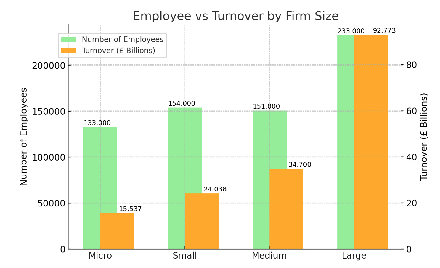
Based on this data, we created our simulated economy where the initial conditions where proportional to real ratios. For example, in the UK (industry code 620) Micro firms represents almost 82% of the industry, employ 20% of the labour and capture a bit more than 9% of the industry turnover. Similarly, large firms represents 0.5% of the number of firms, are the largest employer with almost 35% of the labour force, and capture more than half the total industry turnover. Finally, small and medium business represent 14.5% and 3 % respectively and employ 23% and 22% percent of the labour force.
The table below shows the actual number of firms and workers in our simulation, reflecting the proportions observed in the UK industry in the data.
| Firm Size | No. of Firms | Average Employees per Firm | Capital per Firm (£M) | Total Employees |
|---|---|---|---|---|
| Micro (1–9) | 164 | 3 | 0.36 | 511 |
| Small (10–49) | 29 | 20 | 3.00 | 588 |
| Medium (50–249) | 6 | 97 | 22.00 | 579 |
| Large (250+) | 1 | 847 | 337.00 | 847 |
| Total | 200 | 2,525 | ||
The number of firms and workers in the simulation was set to match the real-world proportional distribution across firm sizes, but the absolute values were scaled down to balance realism with computational efficiency. The cost of each cycle mainly depends on the number of worker–firm interactions and a small sorting term, was approximated as:
| \[T_{\text{cycle}} \propto W m + (W m)\log \frac{W m}{F}\] | \[(1)\] |
| \[\frac{W m}{F} \log\left(\frac{W m}{F}\right)\] | \[(2)\] |
Multiplying by the total number of firms \(F\) gives the total ranking cost across all firms:
| \[F \times \frac{W m}{F} \log\left(\frac{W m}{F}\right) \;=\; (W m) \log\left(\frac{W m}{F}\right)\] | \[(3)\] |
Geffen (2017) compares several pair-matching algorithms in microsimulations and demonstrates how naive approaches (e.g., brute-force \(O(n^2)\)) become infeasible with growing populations, reinforcing the need for more efficient methods like heap-based ranking in ABMs.
In our simulation, firms advertise positions at three levels: junior, medium, and experienced. Employed workers can also apply for these roles, meaning that when promoted, they may choose to move to another company for the same position but with a higher wage. This reflects real-world practice, where wage bands often exist for the same role across different firms. As a result, they compete not only with unemployed jobseekers but also with other employed workers. Without this promotion mechanism, the model would imply that workers never progress in their careers, which would artificially reduce the level of competition for vacancies in each cycle. Wages are segmented by experience tiers.
- Junior: £27,000–£38,000
- Mid-level: £38,000–£47,000
- Experienced: £47,000–£55,000
Firms tend to favour adjusting their WFH offers over increasing wages. This preference is partly driven by the economic incentive to retain, when possible, a larger share of profits: lower wages mean offering a smaller portion of the surplus to workers (Barrero et al. 2022). This decision is also shaped by the learning process itself: firms must trial different strategies multiple times before settling on the one that performs best.
In our simulation, initial worker WFH preferences are drawn from a beta distribution skewed towards fully remote work. Specifically, we sample from:
| \[x \sim \mathrm{Beta}(\alpha = 5, \beta = 2)\] | \[(4)\] |
This skewed behaviour is modelled through weighted random selection, where WFH-related strategies are more likely to be chosen than wage increases. Firms offers different degrees of WFH, but full WFH results in a slightly lower productivity due to reduced collaborative efficiency. UK data from the Office for National Statistics indicates that employees who mainly worked from home were significantly less likely to be promoted, suggesting a real penalty in career progression, possibly due to reduced visibility and informal interaction (Office for National Statistics 2021).
- 1 = Fully remote working.
- 0.75 = Mainly remote working.
- 0.35 = Some elements of remote working, but mainly in office work.
- 0 = Full office work.
Over time, the learning mechanism allows both sides to adapt. Firms may shift their offers if hiring is unsuccessful, while workers may relax their preferences after repeated rejections. This setup captures the negotiation space between supply and demand in terms of working arrangements.
Strategy selection is driven by the average number of positions filled using each option. If a firm consistently fails to hire successfully, the strategy is reset. This mechanism is designed to prevent firms from persisting with approaches that clearly do not work, allowing them to explore alternatives instead of getting stuck in an unproductive loop. While simple, this rule reflects a basic form of adaptive learning under uncertainty.
In our model, workers can receive multiple job offers from multiple firms, but only one per firm per cycle. During each cycle, they evaluate all the offers they have received and, immediately, accept just one (i.e., they are employed to just one firm).
Allowing multiple simultaneous applications (as opposed to just one application per firm per cycle) is a more realistic job search process. Candidates (unemployed or on-the-job-searchers) often consider several positions simultaneously and apply to multiple opportunities before making a decision. In real labour markets, it is common for jobseekers to submit dozens, even hundreds, of applications over time (Financial Times 2024), and this aspect of the simulation mirrors that behaviour.
Job selection is driven by a utility function combining wage and WFH preference. Workers only apply if the utility exceeds their current state. The utility function is defined as below, where the second term represents the satisfaction from matching WFH preference:
| \[ U = \log(\text{wage}) \times \left(1 - \left| \text{WFH}_{\text{preference}} - \text{WFH}_{\text{offer}} \right| \right)\] | \[(5)\] |
To improve the readability of the paper, a detailed explanation of the utility function and the associated plots can be found in Appendix III. The main text presents only the core intuition behind the utility specification, while the appendix provides a fuller discussion of its behaviour under different wage and WFH-preference scenarios.
Although this level of detail may appear unnecessary from a purely computational point of view, it is important for the economic interpretation of the model. The utility function is not just a technical implementation choice; it determines how agents evaluate job offers and therefore shapes the behavioural logic of the simulation. Choosing an inappropriate utility function could generate implausible agent behaviour, distort the interaction between wages and non-monetary preferences, and ultimately lead to misleading aggregate outcomes. For this reason, Appendix III explains why the selected specification is appropriate for the theoretical purpose of the model.
Findings
Results are reported using Monte Carlo averages rather than a single simulation run. Since the model contains stochastic elements in worker search, firm hiring, and strategy adaptation, one run would only represent one possible realisation of the labour market. Repeated runs therefore provide a more stable baseline against which the Non-WFH and WFH models can be compared. For ease of exposition,full sensitivity results are reported separately in Appendix IV.
Table 6 compares the baseline outcomes of the simulation without WFH preferences and the simulation with WFH preferences included. The comparison is not to claim that WFH mechanically improves all labour market outcomes, but rather to examine how the inclusion of WFH as a non-wage job attribute changes the behaviour of the model.
| Indicator | Non-WFH Baseline | WFH Baseline |
|---|---|---|
| Unemployment rate | 0.0338 | 0.0369 |
| Average wage multiplier | 1.3731 | 1.2129 |
| Average worker utility | 10.2679 | 10.2289 |
The unemployment rate is slightly higher in the WFH baseline, increasing from 0.0338 in the Non-WFH model to 0.0369 in the WFH model. This difference is relatively small and it suggests that the introduction of WFH preferences does not fundamentally alter the aggregate employment level in the baseline simulation.
Average worker utility is also very similar across the two models. In the Non-WFH baseline, average worker utility is 10.2679, compared with 10.2289 in the WFH baseline. This small difference shows that the inclusion of WFH preferences does not, by itself, generate a large improvement in aggregate worker utility. This is an important point. WFH does not increase utility simply because it has been added to the model. What matters is whether the worker’s preference is matched by the firm’s offer. In other words, it is the match or mismatch between preferences and job attributes that affects utility, rather than the mere presence of an additional job attribute. Indeed, one could argue that introducing more expectations into the employment relationship may reduce overall satisfaction when those expectations are not met. For this reason, the WFH model should not be interpreted as automatically making workers better off; rather, it shows that non-monetary preferences can shape utility positively or negatively depending on how well they are matched in the labour market.
One notable difference is observed in the average wage multiplier. In the Non-WFH baseline, the wage multiplier is 1.3731, meaning that workers require a wage offer approximately 37.31% above their current wage before accepting a move. In the WFH baseline, this falls to 1.2129, meaning that workers require approximately 21.29% above their current wage. This represents a reduction of around 16.02 percentage points in the required wage premium.
The results suggest that WFH acts as a compensating non-monetary attribute within the bargaining process. Without WFH, firms may need to offer higher wages to attract comparable candidates. When WFH is available, however, firms can improve the attractiveness of a vacancy without relying exclusively on salary increases. They may therefore maintain wages close to the industry average while offering greater flexibility, or raise wages by less than would otherwise be necessary. For workers, this would be the equivalent of trading part of the wage premium for a job offer that better matches their non-monetary preferences. For example, for a worker currently earning £40,000, the Non-WFH baseline requires a new wage of approximately £54,924, while the WFH baseline requires approximately £48,516, a difference of around £6,408.
The economic significance of this result is potentially important given the size of the sector being modelled. The UK computer programming, consultancy and related activities sector contains a large number of firms and employees, with substantial aggregate turnover. Therefore, even relatively small changes in wage premium or job switching thresholds have meaningful implications when considered at sector level.
The baseline comparison suggest that WFH reduces wage pressure in the simulated labour market. In the Non-WFH baseline, workers require a wage multiplier of 1.3731 to move, equivalent to a wage premium of 37.31%. In the WFH baseline, this falls to 1.2129, equivalent to a wage premium of 21.29%. The difference of 0.1602 represents a reduction of 16.02 percentage points in the required wage premium.
| Share of Workers Affected | No. of Workers Affected | Illustrative Reduction (£ millions) | Illustrative Reduction (£ billions) |
|---|---|---|---|
| 5% | 33,550 | 214.99 | 0.215 |
| 10% | 67,100 | 429.98 | 0.430 |
| 20% | 134,200 | 859.95 | 0.860 |
| 30% | 201,300 | 1,289.93 | 1.290 |
| 100% | 671,000 | 4,299.77 | 4.300 |
Source: Employment data from the Business Population Estimates 2023 Business Population Estimates (2023). Author's calculation based on simulation results.
For example, for a worker currently earning £40,000, this corresponds to a reduction of approximately £6,408 in the wage increase required to accept a new job. Applied illustratively to the 671,000 employees in SIC 620, this would correspond to an upper-bound reduction in required wage premia of approximately £4.3 billion. This should not be interpreted as a direct payroll saving, since not all workers move jobs in a given period. Instead, it indicates the potential scale of reduced wage pressure when WFH operates as a compensating non-wage job attribute.
Behavioural outcomes results
Figure 2 summarises the distribution of the main WFH baseline outcomes across the Monte Carlo runs. The results show that firms converge towards relatively high levels of WFH provision, with mean WFH rates of approximately 0.846 for micro firms, 0.873 for small firms, and 0.811 for medium firms. Average worker utility remains concentrated around 10.229, while the average wage multiplier is around 1.213. This suggests that, in the WFH baseline, workers still require a wage premium to move jobs, but this premium is lower than in the Non-WFH version of the model.
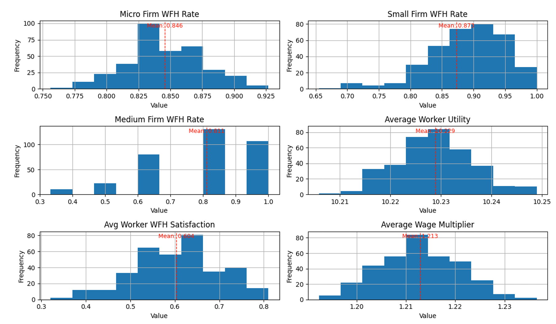
Figure 3 shows the distribution of WFH satisfaction by worker experience level. Most workers are concentrated in the 0.6–0.8 satisfaction range, with a smaller but still important group in the 0.8–1.0 range. The figure reflects both satisfaction outcomes and the number of workers in each experience group. The dominance of senior workers in the chart does not necessarily mean that senior workers are always more satisfied, but rather that they represent a large share of the observed worker population in the simulation.
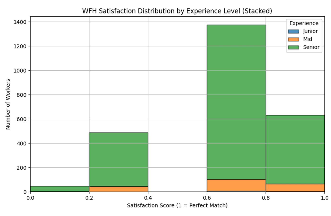
Figure 4 presents the same satisfaction distribution by firm size. Again, most workers are concentrated in the higher satisfaction ranges, especially between 0.6 and 1.0. Large firms account for many of the workers in the 0.6–0.8 band, while micro and medium firms also contribute visibly to the higher satisfaction categories. This suggests that WFH matching is not limited to one firm size category, although the distribution is naturally affected by the number of workers employed by each type of firm.
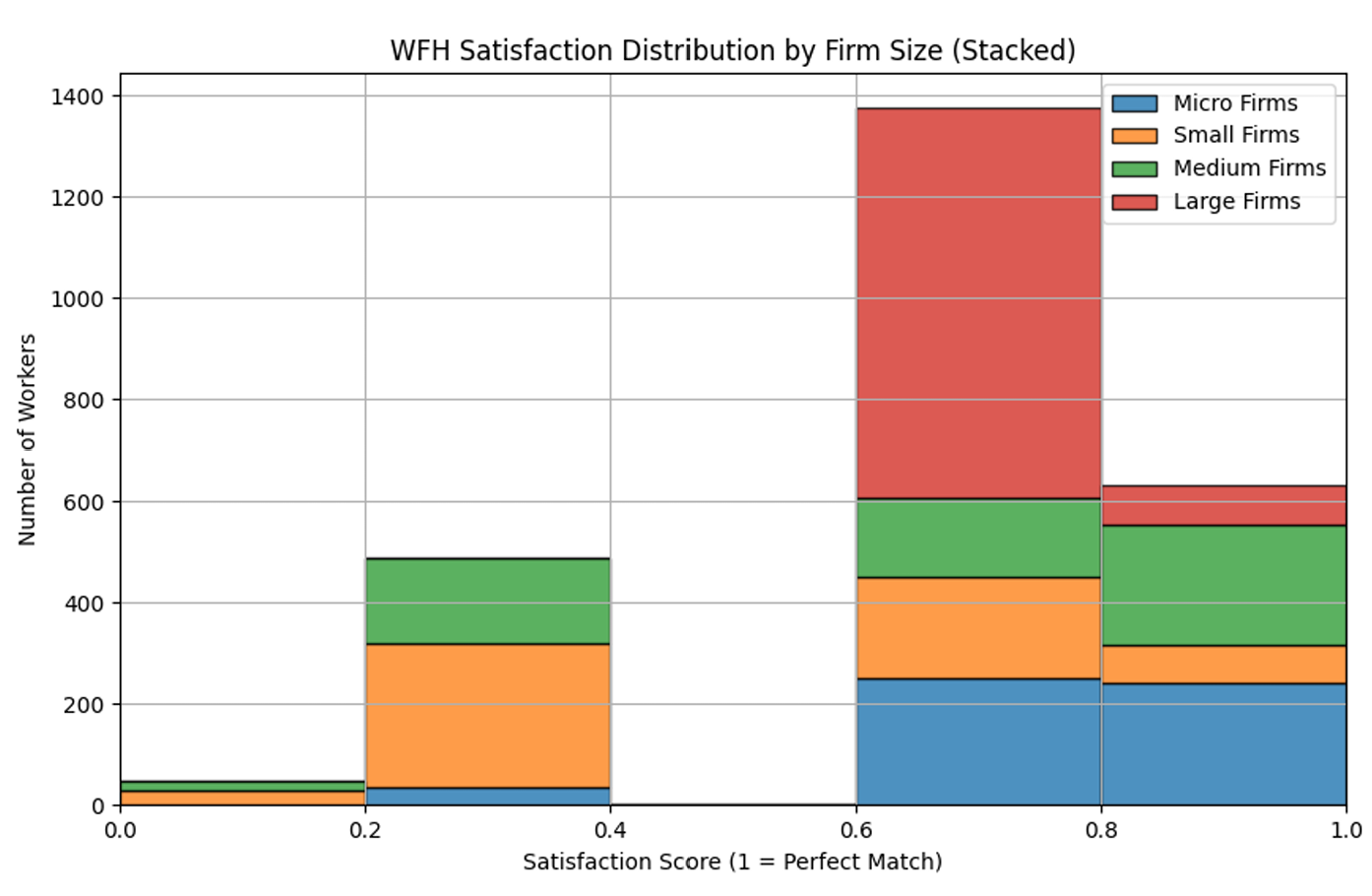
Figure 5 shows the overall distribution of worker WFH satisfaction scores. The largest group of workers is located in the 0.6–0.8 range, followed by a substantial group in the 0.8–1.0 range. Only a small number of workers fall close to zero satisfaction. Broadly speaking, this suggests that the WFH baseline produces a moderate to high level of WFH preference matching for most workers, although the match is not perfect for everyone.
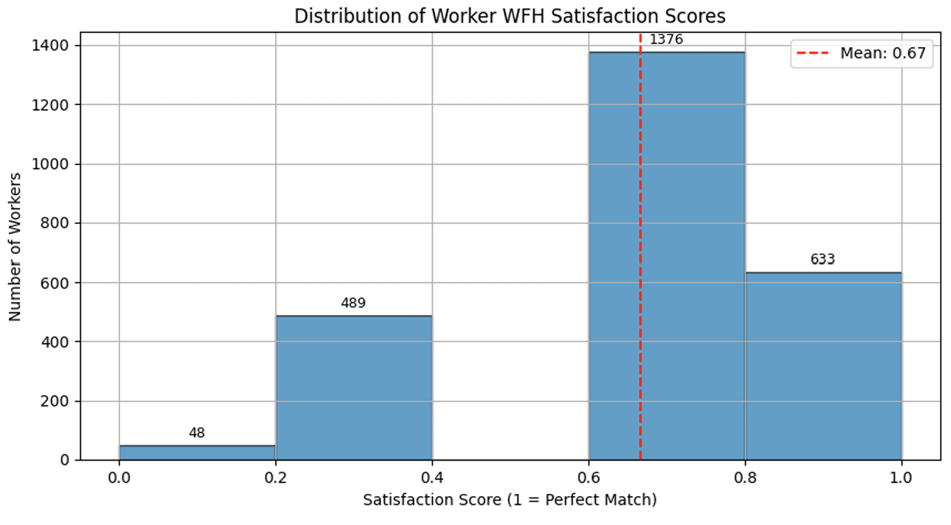
Overall, the main WFH baseline results suggest that the introduction of WFH preferences creates a labour market in which firms tend to offer relatively high levels of WFH and most workers achieve at least moderate WFH satisfaction. At the same time, the results should not be read as showing that WFH solves all matching frictions. Some mismatch remains, and average satisfaction is below the perfect-match value of 1. A cautious conclusion is that WFH acts as an important non-monetary job attribute in the model, improving the scope for preference matching while also reducing the wage premium required for workers to move jobs.
Our simulation showed that while wages are largely determined by the market, non-monetary incentives like working from home can significantly improve recruitment outcomes especially in knowledge intensive industries. In sectors where wage flexibility is limited (i.e., where, on average, wages for a given role are mainly determined by market forces of supply and demand and therefore do not deviate significantly from the competitive benchmark), negotiating around personal preferences becomes a vital growth strategy. This stands in contrast with less mature or distorted labour markets, where wages are not primarily defined by market conditions but instead shaped by institutional rules, bargaining asymmetries, or structural frictions, often leading to compensation levels that diverge from market-driven benchmarks.
Our findings answer a broader question: in industries where salaries are largely governed by competitive dynamics, how can firms attract new talent without compromising their profit margins? The answer lies in engaging with workers’ personal preferences. Whether through remote work or, in the near future, shorter work weeks, firms operating in such mature markets should be encouraged to adopt these practices to sustain growth.
Worker satisfaction and utility are highest when wage expectations are balanced and firms offer strong or flexible WFH options. Workers’ overly conservative or overly ambitious expectations reduce satisfaction. Changes in application limits and job visibility affect matching outcomes, but the direction and size of these effects are modest and not always monotonic. Firm strategies remain stable under most conditions, but become more diverse when worker expectations rise.
A possible concern is that the conclusions regarding worker satisfaction and utility are built into the model by the behavioural rules, and therefore not genuine outcomes of the simulation. We argue that this is not the case. Worker satisfaction cannot be meaningfully evaluated without a measure of satisfaction, and in economics, one of the most accepted and conventional measure is the utility function (Samuelson 1947). Regardless of the specific shape of the utility function or the exact formulation we employ, the results we observe remain indicative. For instance, the findings that overly conservative or overly ambitious wage expectations reduce satisfaction follow from the interaction of agents within the simulated market, rather than being predetermined.
Moreover, omitting the use of a utility function altogether would be unconventional and would require explicit justification for adopting an alternative technique to represent personal preferences (such as work-from-home intensity). In this sense, the results are not tautological, but instead reflect emergent outcomes from the interaction of workers and firms under the defined conditions.
Model Documentation, Code Availability and Reproducibility
The model has been documented and archived to allow other researchers to inspect, run, and extend the simulation. The full implementation is available through the CoMSES Computational Model Library at: https://www.comses.net/codebase-release/25119713-c007-4ed7-9d99-f71f3e5e9056/ and through the accompanying GitHub repository. The CoMSES documentation provides a structured description of the model, including its purpose, scope, entities, state variables, scheduling, design concepts, submodels, assumptions, pseudocode, model outputs, verification checks, validation approach, and possible experiments. The GitHub repository contains the Python source code, environment files, model scripts, output structure, and run instructions used to generate the results reported in this paper.
The paper reports Monte Carlo simulation outputs rather than relying on one isolated simulation path. Reproducibility is supported in three ways. First, the model can be run using fixed random seeds, so that the same parameter configuration can be reproduced. Second, the baseline and sensitivity-analysis settings are explicitly reported in the manuscript. Third, the repository includes the terminal commands used to run the main experiments, together with the corresponding output folders and log files.
The main WFH baseline reported in the paper was generated using 300 Monte Carlo runs with 8 simulation cycles per run. The non-WFH baseline was generated using the same number of Monte Carlo runs and cycles, allowing the two baseline scenarios to be compared under the same simulation structure. The sensitivity analyses were generated using 100 Monte Carlo runs per scenario, again with 8 simulation cycles per run unless otherwise stated. This design was chosen to balance computational feasibility with the need to test whether the main patterns remain stable under alternative behavioural and search assumptions.
The model can be reproduced by running the simulation from the terminal using the scripts provided in the repository. The general structure of the command is:
conda run -n abm-sim-env python mainslr.py --montecarlo --runs N --cycles C --noguiwhere N is the number of Monte Carlo runs and C is the number of simulation cycles. For example, the WFH baseline can be reproduced using:
conda run -n abm-sim-env python mainslr.py --montecarlo --runs 300 --cycles 8 --noguiThe same structure is used for the sensitivity analysis, changing only the relevant parameter in the source code or configuration before running the experiment. The parameters varied in the sensitivity analysis include worker wage expectation, maximum applications per year, job visibility, firm strategy weights, and the unemployment-duration threshold before workers enter desperation mode. All other baseline settings are kept constant when one parameter is varied.
The principal output files generated by the model include cycle-level logs, firm and worker records, job advertisement records, rejection logs, Monte Carlo summary files, seed records, and plots used to construct the figures and tables in the paper. The model records both individual-level and aggregate outcomes. These include unemployment rate, number of employed workers, number of vacancies, number of unfilled vacancies, wage multipliers, WFH offers by firm size, worker utility, WFH satisfaction, hiring success, and Monte Carlo distributions across repeated runs.
Contributions and Limitations
One of the key contributions of this work lies in its ability to simulate and track the evolution of hiring strategies, allowing for a nuanced comparison between monetary (wage-based) and non monetary (WFH-based) decision making. Our results show that while wages tend to remain anchored to industry norms, flexibility around remote work offers significant strategic value, especially in attracting and retaining talent.
Recent evidence suggests that remote and hybrid work should not be treated as a marginal employment benefit, but as an important component of labour matching. Gallup reports that, among employees in remote-capable jobs, six in ten prefer a hybrid work arrangement, around one-third prefer fully remote work, and fewer than 10% prefer to work fully on-site. The same source reports that, among remote-capable jobs, 26% of workers are exclusively remote, 52% are hybrid, and 22% are on-site (Gallup 2026). These figures suggest that work-from-home flexibility has become a central characteristic of employment, rather than a temporary or secondary feature of post-pandemic labour markets.
This is particularly relevant for the behavioural assumptions of the model. Gallup also reports that six in ten remote-capable employees who currently work exclusively remotely would be extremely likely to look for another job if remote flexibility were removed (Gallup 2026). This indicates that, for a significant proportion of workers, remote flexibility enters the job decision very strongly. In the context of this model, this supports the assumption that workers do not evaluate job offers through wages alone. Instead, they assess a wider bundle of job attributes, where flexibility, autonomy, and work-life balance can materially affect utility. these non-monetary characteristics are strong enough to influence whether a worker remains in a job, rejects an offer, or searches for alternative employment.
Employer-side evidence points in a similar direction. The ZipRecruiter employer survey (ZipRecruiter 2024) reports that, among companies experiencing reduced turnover, 47% attributed this to enhanced job security and stability, while 46% pointed to better work-life balance policies. Other commonly cited explanations included improved benefits and compensation packages, career development opportunities, employee engagement and satisfaction, recruitment practices, company culture, onboarding, and formal retention programmes . This does not imply that wages are irrelevant. Instead they show that labour mobility and retention cannot be explained by pay alone. Work-life balance in the survey is consistent with the interpretation developed in this paper, where workers respond to non-monetary job characteristics and firms may improve matching outcomes by adjusting employment conditions beyond wages.
The broader remote-work statistics reported by Forbes also support the choice of this topic as a relevant setting for the study. The article reports that 16% of companies operate fully remotely and that 98% of workers would like to work remotely at least some of the time (Haan 2026). Although this source is used here as contextual evidence rather than as a primary academic source, these figures help illustrate the scale of remote work preferences in modern labour markets. They suggest that working from home is not a niche preference, but a widespread expectation among workers. This makes it reasonable to include work-from-home preferences as a meaningful matching variable alongside wage expectations in industries where remote working is possible.
This is especially important in labour markets where wages may not adjust freely enough to capture all differences in worker preferences. If wage offers are constrained by internal pay structures or industry averages, then non-monetary job attributes become more significant. Under these conditions, working form home flexibility becomes an alternative margin of competition between firms. Firms may not always be able or willing to raise wages substantially, but they may still compete through flexibility, work-life balance, autonomy, and working conditions. This provides a strong theoretical reason for modelling working from home preferences as part of the worker utility function rather than treating it as a minor addition to wage based matching.
From the firm’s perspective, remote and hybrid work operates as a recruitment and productivity strategy. Penn LPS Online (Penn LPS Online 2025) notes that remote work allows firms to access a wider talent pool, recruit beyond local labour markets, and address skill gaps by hiring workers with specialised knowledge regardless of location. It highlights potential benefits for productivity and employee satisfaction when remote work is managed effectively .
Taken together, these sources support the central assumption that labour-market matching is not determined by wages alone. Wages remain important, but workers also evaluate jobs through flexibility, autonomy, work-life balance, and the compatibility between job arrangements and personal preferences. For firms, offering work-from-home arrangements may therefore become part of the hiring strategy, particularly when wage competition is limited or when firms face difficulty attracting suitable candidates. The evidence is consistent with the model’s treatment of working from home as a meaningful behavioural and strategic variable in labour market matching.
The main theoretical contributions are:
- WFH becomes a recruitment strategy, not only a worker preference. The model shows that WFH is not simply something workers prefer. Once firms experience hiring failure, WFH becomes part of their adaptive recruitment strategy. Firms adjust WFH offers because previous strategies did not attract enough suitable workers.
- WFH acts as a non-monetary compensating job attribute. The model shows that firms can make vacancies more attractive by changing working arrangements, rather than relying only on higher salaries. WFH therefore becomes part of the overall job offer.
- WFH can reduce wage pressure Workers can achieve similar utility levels even when wage multipliers do not increase substantially, because utility comes from both wage and the match between the worker’s WFH preference and the firm’s WFH offer.
- WFH can partially substitute for wage competition. In a segmented labour market, firms do not need to compete only through wages. They can also compete through flexibility. This means WFH can reduce the need for large wage increases while still improving matching outcomes.
- Firm-size differences emerge from the model. Micro, small, medium, and large firms may settle on different WFH strategies because they face different growth rates, vacancy pressures, hiring constraints, and productivity conditions.
- Matching improves through repeated adaptation, not instant market clearing. Workers adjust expectations after failed searches, and firms adjust strategies after failed hiring attempts. Matching improves gradually through repeated cycles.
- Search frictions matter. Workers do not see all jobs, and firms do not receive applications from all workers. Therefore, the same preferences can lead to different outcomes depending on job visibility, application limits, and vacancy distribution.
- The macro-level outcome emerges from interaction effects. The model does not simply assume that WFH improves outcomes. The aggregate pattern emerges from repeated local interactions between workers and firms, where preferences, wages, vacancies, search limits, and learning rules jointly shape the final labour-market result.
Despite these strengths, the model has limitations. First, the current implementation is specific for the UK IT sector and does not account for inter industry differences, regional labour market variations, or broader macroeconomic shocks. The decision to focus on a relatively stable sector was deliberate, but it means that results may not generalise across other parts of the economy where external volatility or regulation plays a stronger role.
Second, while the model includes realistic behavioural rules and wage segmentation, it simplifies other aspects such as firms reputation, unusual contract types, or part-time vs. full-time roles. These exclusions may or may not influence utility outcomes in real world settings.
Third, the firm learning mechanism does not yet account for peer imitation, strategic coordination across firms, or long term memory. Incorporating more sophisticated learning models may yield additional insights, particularly in settings where firms actively benchmark against one another.
Hiring strategies in the current model are driven by firms’ need to balance wage offers and work-from-home (WFH) options in order to attract workers. These strategies are not arbitrary but directly shaped by workers’ personal preferences: a firm that consistently offers wages below expectations or rigid WFH arrangements risks unfilled vacancies, while firms that align better with worker preferences improve their hiring outcomes. In this sense, hiring strategies can be seen as adaptive responses to the distribution of preferences in the labour market.
Our model treats capital and productivity only in aggregate terms, abstracting from firm specific capital accumulation or investment choices. This means that all firms of a given size operate under broadly similar productivity constraints, and wage or WFH strategies are not directly tied to investment behaviour. Introducing capital heterogeneity (allowing firms to build, allocate, and invest capital differently), would provide a more realistic link between investment decisions and hiring strategies.
A capital rich firm, for example, could afford higher wages or more flexible WFH offers as part of its recruitment strategy, whereas a capital constrained firm might need to rely on stricter wage discipline or more conservative offers. In turn, this would sharpen the connection between structural firm characteristics (capital, productivity) and the micro-level process of preference matching (wages, WFH), providing richer insights into how firms compete for talent under heterogeneous financial and technological conditions.
Acknowledgements
We would like to express our deep gratitude to Professor Nigel Gilbert for his generosity in sharing his expertise and for the invaluable one-to-one conversations that greatly improved the clarity and depth of this work. We also thank our colleagues from the Birkbeck Institute for Data Analytics for their valuable feedback and insightful discussions. This research was supported by the SoCMS GTA programme.
Notes
- Although definitions vary, Blanchard (1997) talks about the medium run as a transition period that is not the same as the short-term business cycle or the long-term growth trend. Other sources (Investopedia 2025), give similar descriptions. CEDEFOP (2024) uses five years as their standard medium-term forecast horizon. So an eight-year simulation, where each cycle is one year, still sits well inside what is normally seen as the medium term in both labour economics and strategic business planning.↩︎
Appendix I: Full Cycle Flow Chart
Appendix II: The Programming Platform and Model Stability
The programming platform
The simulation was developed in Python. It is executed from the command line, enabling headless execution. Suitable for batch runs, including Monte Carlo experiments and integration with high-performance computing environments such as SLURM clusters.
To support transparency and reproducibility, the full source code has been deposited in the CoMSES Net Computational Model Library, where it can be accessed, reused, and extended by other researchers (https://www.comses.net/codebase-release/d2353c9e-a578-45a4-8599-4523dedf73c5/).
Each cycle represents one year and follows the process detailed in Appendix I. One complete full simulation is 8 years. This aligns with standard definitions of the medium term in labour economics and business strategy.1
This duration is sufficient to observe meaningful adaptations in firm and worker behaviour (e.g., experience accumulation, wage strategy shifts) while remaining short enough to avoid speculative effects of long-term dynamics like economic shocks. Longer horizons risk being distorted by external shocks (e.g., crises, policy changes), which are deliberately excluded from this model’s scope.
Our simulation was run twice: with and without working-from-home (WFH) characteristics. The goal is to compare outcomes under the presence or absence of personal preferences. By subsequently comparing each version of the model to real-world data or established economic theory, we aim to identify which configuration more closely resembles observed phenomena.
Model stability
The robustness of our model is then evaluated by examining whether the results remain stable across multiple runs: 350 full simulations, each consisting of 8 cycles (2,800 total cycles), run twice-once with and once without personal preferences (5,600 cycles in total). To assess the stability and reliability of the results across runs, we use the coefficient of variation (CV) (Abdi 2010). Although it is a widely used statistic across disciplines, to our understanding there is no single universally agreed criterion regarding which values of CV are considered good or bad values.
In general, the interpretation tends to follow the rule of thumb that the lower the CV, the better the stability of the measurement, although it remains difficult to specify precise thresholds. Beyond its role as a descriptive statistic, CV has been applied in diverse computational and applied domains, such as time-series change detection, feature selection in neural systems, and in laboratory quality control where it serves as a benchmark for method performance (Chaudhari & Thakkar 2023; Koeniguer & Nicolas 2020).
For the three main metric (worker satisfaction, wage multiplier and firm WFH offer) we computed the CV across all runs. To remain on the side of precaution, we classify values of 10% or lower as stable or very stable, and anything higher than this threshold as indicative of high variability. As a rule of thumb, we have considered CV values below 5% as highly stable, while values between 5% and 10% still indicate low variability and acceptable robustness.
| Metric | CV | Interpretation |
|---|---|---|
| AvgWageMultiplier | 0.0065 | Highly Stable |
| AvgFirmWFH | 0.379 | High variability |
| AvgWFHSatisfaction | 0.1548 | Medium variability |
| Metric | CV | Interpretation |
|---|---|---|
| AvgWageMultiplier | 0.0050 | Highly stable |
Appendix III: The Utility Function
To assess how well firms meet workers’ preferences for remote work, we define a WFH satisfaction score for each employed worker \(i\) as follows:
| \[s_i = 1 - \left| p_i - o_i \right|,\] | \[(6)\] |
where:
- \(p_i \in \{0, 0.35, 0.75, 1.0\}\) is the worker’s WFH preference,
- \(o_i \in \{0, 0.35, 0.75, 1.0\}\) is the WFH offer from the employing firm.
This formulation yields \(s_i = 1\) when a worker’s preference exactly matches the firm’s offer, and \(s_i = 0\) when there is complete mismatch.
We compute the average WFH satisfaction across all employed workers at the end of each simulation cycle using:
| \[\text{AvgWFHSatisfaction} = \frac{1}{N} \sum_{i=1}^{N} s_i,\] | \[(7)\] |
where \(N\) is the total number of employed workers. This metric ranges from 0 (total dissatisfaction) to 1 (perfect alignment between firms and workers).
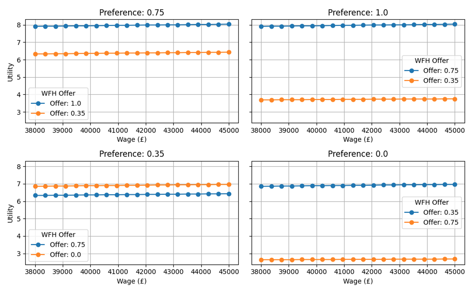
The plot below shows that in our utility function, income is essential, and its marginal utility diminishes as wages increases. This is implemented by using a logarithmic transformation of wage, reflecting the economic principle that additional income has decreasing marginal returns on utility. That is, a £2,000 increase matters more to someone earning £30,000 than to someone earning £60,000.
Mismatch in working conditions reduces perceived utility, not absolutely but proportionally. The satisfaction with WFH arrangements is captured by a linear penalty: the further the firm’s WFH offer is from the worker’s ideal preference, the less utility they derive from the job. Additionally, different workers value WFH differently. The model respects this by letting WFH preferences vary across agents, which shapes their perceived utility even for identical wages.
The simulation begins with a fixed pool of unemployed workers, divided into two categories: those with prior work experience and those without (recent graduates). As the simulation progresses, individuals in this pool can either secure employment and exit unemployment or remain in their current state. Because this model does not incorporate macroeconomic shocks, employed workers cannot be made redundant and return to the unemployment pool.
This assumption follows the design choice seen in simplified agent-based labour market models, where employment dynamics are isolated from exogenous shocks in order to focus on matching processes and behavioural adjustments (Fagiolo et al. 2004). This approach allows for a clearer examination of how preferences, search strategies, and firm behaviour affect unemployment, without the confounding effects of cyclical downturns or policy interventions.
After three cycles unemployed, workers enter “desperation mode” where they are more likely to lower their WFH expectations. This introduces adaptive behaviour driven by unemployment duration, not just static preferences. Workers track the performance of their strategies across cycles and choose the best-performing one to guide future decisions, akin to reinforcement learning (Dehkordi 2023). Performance is measured by the number of offers received over attempts:
| \[\text{success rate} = \frac{\text{offers_received}}{\text{attempts}}\] | \[(8)\] |
Workers do not accept offers below their current wage. This encodes realistic wage rigidity when employed and avoid workers to change jobs after minimal wage improvements. The wage floor is calculated as:
| \[\text{wage}_{\text{floor}} = \text{current_wage} \times 1.10\] | \[(9)\] |
Workers remember their initial WFH preference and are not allowed to reduce it more than one level below the starting point, showing strong preferences but with a certain degree of flexibility. In simpler words, workers preferences for WFH remains sticky even under tight labour market conditions (Drake et al. 2025).
Appendix IV: Sensitivity Analysis
Each free parameter was tested against outcomes related to WFH preferences (on both sides, firms and workers): the rate of WFH offers by firm size (Micro WFH, Small WFH, and Medium WFH), average worker utility, average WFH satisfaction (measured as the difference between the level of WFH desired and the level received), and the wage multiplier from the firm side.
Sensitivity analysis plan
For firms
| Scenario | Runs | Weights (Wage / ↑WFH / ↓WFH) | Purpose |
|---|---|---|---|
| Baseline - WFH Focused - | 350 | (0.10 / 0.45 / 0.45) | Favour non-monetary strategies over wage increases |
| Even Weights | 100 | (0.33 / 0.33 / 0.34) | Neutralise selection to test pure adaptation dynamics |
| Wage-Focused | 100 | (0.70 / 0.15 / 0.15) | Test wage-heavy learning and profitability effects |
For workers
| Scenario | Runs | Initial Multiplier | Purpose |
|---|---|---|---|
| Baseline | 350 | 1.10 | Default wage expectation behaviour (10% above current wage) |
| Low Expectation | 100 | 1.00 | Test worker outcomes when expectations align exactly with current wage |
| Optimistic Workers | 100 | 1.25 | Evaluate effects of ambitious wage demands on employment |
| Pessimistic Workers | 100 | 0.95 | Explore job access when wage expectations are conservative |
| Scenario | Runs | Cycles Unemployed | Purpose |
|---|---|---|---|
| Baseline | 350 | 3 cycles | Trigger expectation drop after 3 cycles of unemployment |
| Early Desperation | 100 | 1 cycle | Observe job matching if workers adjust too quickly |
| Delayed Desperation | 100 | 5 cycles | Evaluate prolonged search with unchanged expectations |
| No Desperation Mode | 100 | Infinite | Disable desperation entirely to test robustness of search behaviour |
| Scenario | Runs | Application Cap | Purpose |
|---|---|---|---|
| Baseline | 350 | 300 | Allow wide but finite search reach per cycle |
| Conservative Search | 100 | 150 | Model workers with narrower job search effort |
| Aggressive Search | 100 | 500 | Simulate high job search intensity |
| Scenario | Runs | Visibility Range | Expected Effect |
|---|---|---|---|
| Baseline | 350 | 80% – 95% | Workers see a high proportion of job ads; moderate matching frictions |
| Low Visibility | 100 | 40% – 60% | Increases search frictions; more mismatch and longer unemployment |
| Full Visibility | 100 | 100% | Perfect information; market clears efficiently but unrealistically |
| High Noise | 100 | 60% – 100% | Mixed access to jobs; higher variance in outcomes |
Sensitivity analysis results
Here we clarify how the main reported indicators should be interpreted. The values in the table are aggregate simulation outcomes rather than observations for a single firm or worker. In particular, the WFH values are averages across firms and simulation runs, even though individual firms select from a discrete set of WFH strategies.
| Indicator | Scale / Possible Values | Interpretation |
|---|---|---|
| Micro WFH, Small WFH, Medium WFH | Firm WFH offers are selected from four discrete values: \(0\), \(0.35\), \(0.75\), and \(1.00\). | These columns report the average WFH offer made by firms of each size category. For example, a value of \(0.845\) for micro firms does not mean that an individual firm offers exactly \(0.845\) WFH. Rather, it is an average across firms and simulation runs. It indicates that micro firms are, on average, offering a high level of WFH, between mainly remote work and fully remote work. |
| Worker Utility | Model-generated utility score. Not a percentage. | This value represents the average utility achieved by workers. In the model, utility combines wage income with the degree of match between the worker’s WFH preference and the firm’s WFH offer. Higher values indicate better worker outcomes, but the figure should be interpreted comparatively across scenarios rather than as a direct monetary value. |
| WFH Satisfaction | Ranges from \(0\) to \(1\). | This measures the average alignment between workers’ preferred WFH level and the WFH level offered by their employer. A value of \(1\) means a perfect match, while \(0\) means complete mismatch. For example, a value of \(0.603\) means that workers achieve, on average, around \(60.3\%\) of the maximum possible WFH match. |
| Wage Multiplier | Multiplier above the worker’s current wage. | This indicates the minimum wage premium required for a worker to accept a move to a new employer. For example, a value of \(1.212\) means that the worker would require a wage offer at least \(21.2\%\) above their current wage before accepting a new job. |
Table 16 - 20 presents the results of this analysis. The values shown in blue are both the results and the initial settings used in our base scenario. These are highlighted for the reader’s benefit when comparing the base scenario against the sensitivity analysis outcomes.
| Scenario | Micro WFH | Small WFH | Medium WFH | Worker Utility | WFH Satisfaction | Wage Multiplier |
|---|---|---|---|---|---|---|
| This table measures how changing the worker wage expectation parameter affects firm WFH offers, worker utility, WFH satisfaction, and the wage premium required by workers to move jobs. | ||||||
| Worker Wage Expectation at 1.10 | 0.845 | 0.872 | 0.811 | 10.228 | 0.603 | 1.212 |
| Worker Wage Expectation at 1.00 | 0.841 | 0.885 | 0.873 | 10.221 | 0.608 | 1.213 |
| Worker Wage Expectation at 0.95 | 0.847 | 0.880 | 0.816 | 10.207 | 0.596 | 1.214 |
| Worker Wage Expectation at 1.25 | 0.847 | 0.879 | 0.840 | 10.231 | 0.596 | 1.208 |
| Scenario | Micro WFH | Small WFH | Medium WFH | Worker Utility | WFH Satisfaction | Wage Multiplier |
|---|---|---|---|---|---|---|
| This table measures the effect of changing the maximum number of job applications workers can make per year. It tests whether greater or lower search intensity changes firm strategies and worker outcomes. | ||||||
| Max 300 Applications per Year | 0.845 | 0.872 | 0.811 | 10.228 | 0.603 | 1.212 |
| Max 500 Applications per Year | 0.853 | 0.875 | 0.838 | 10.230 | 0.592 | 1.212 |
| Max 150 Applications per Year | 0.850 | 0.888 | 0.804 | 10.230 | 0.618 | 1.212 |
| Scenario | Micro WFH | Small WFH | Medium WFH | Worker Utility | WFH Satisfaction | Wage Multiplier |
|---|---|---|---|---|---|---|
| This table measures how changing workers' visibility of available job advertisements affects matching outcomes. Higher visibility means workers can observe a larger share of available jobs before applying. | ||||||
| Job Visibility 80–95% | 0.845 | 0.872 | 0.811 | 10.228 | 0.603 | 1.212 |
| Job Visibility 40–60% | 0.832 | 0.873 | 0.808 | 10.314 | 0.632 | 1.172 |
| Job Visibility 60–100% | 0.850 | 0.874 | 0.826 | 10.239 | 0.598 | 1.208 |
| Job Visibility 100% | 0.843 | 0.890 | 0.871 | 10.197 | 0.602 | 1.227 |
| Scenario | Micro WFH | Small WFH | Medium WFH | Worker Utility | WFH Satisfaction | Wage Multiplier |
|---|---|---|---|---|---|---|
| This table measures the effect of changing the probability distribution used by firms when experimenting with WFH strategies. It shows whether different initial strategy tendencies affect final WFH offers and worker outcomes. | ||||||
| WFH Strategy 0.10–0.45–0.45 | 0.845 | 0.872 | 0.811 | 10.228 | 0.603 | 1.212 |
| WFH Strategy 0.34–0.33–0.33 | 0.851 | 0.730 | 0.700 | 10.230 | 0.633 | 1.243 |
| WFH Strategy 0.70–0.15–0.15 | 0.850 | 0.680 | 0.666 | 10.230 | 0.704 | 1.263 |
| Scenario | Micro WFH | Small WFH | Medium WFH | Worker Utility | WFH Satisfaction | Wage Multiplier |
|---|---|---|---|---|---|---|
| This table measures how changing the number of unsuccessful job-search cycles before workers lower their expectations affects worker outcomes and firm WFH offers. | ||||||
| Desperation Threshold 3 Cycles | 0.845 | 0.872 | 0.811 | 10.228 | 0.603 | 1.212 |
| Desperation Threshold 5 Cycles | 0.845 | 0.878 | 0.810 | 10.228 | 0.627 | 1.214 |
| Desperation Threshold 1 Cycle | 0.847 | 0.867 | 0.843 | 10.228 | 0.617 | 1.212 |
| No Desperation Mode | 0.846 | 0.868 | 0.860 | 10.230 | 0.620 | 1.213 |
While some variation can be observed across the different scenarios, in most cases these changes are relatively small and should be interpreted cautiously. Given that the model relies on Monte Carlo simulations, part of the observed variation between one scenario and another may simply reflect stochastic uncertainty introduced by the simulation process itself rather than a direct behavioural effect caused by the parameter change.
These results show that the main outcomes of the model remain stable across the tested parameter ranges. Changes to worker wage expectations, the maximum number of applications per year, job visibility, and the desperation threshold produce only modest differences in aggregate outcomes. Average WFH offers across firm sizes remain relatively close to the baseline scenario, worker utility changes only marginally, and the wage multiplier also remains within a fairly narrow range. In this sense, the sensitivity analysis provides evidence that the main findings of the model are not being driven by a single arbitrary calibration choice.
This does not mean that the parameters themselves are unimportant, but rather that small changes within the ranges tested here do not fundamentally alter the broader dynamics of the labour market generated by the model. For this reason, the results should not be over interpreted. For example, although some scenarios show slightly higher utility or satisfaction outcomes, the sensitivity analysis by itself does not allow us to conclude with certainty that these changes are caused by a specific behavioural mechanism. In many cases the differences are simply too small to separate confidently from the level of uncertainty naturally introduced by repeated stochastic simulations.
The clearest differences can be observed in the scenarios relating to firms WFH strategy probabilities. Unlike the other sensitivity tests, these scenarios produce more visible changes, particularly in the WFH offers of small and medium-sized firms. Under the baseline strategy distribution, small and medium firms report average WFH offers of 0.872 and 0.811 respectively. When the strategy probabilities are changed to 0.33–0.33–0.34, these values fall to 0.730 and 0.700. Under the 0.70–0.15–0.15 distribution, they fall further to 0.680 and 0.666.
Compared to the other sensitivity tests, these changes are noticeably larger. This is explained by the way firms adapt and experiment with WFH strategies is a more influential modelling assumption than some of the worker-side behavioural thresholds tested elsewhere in the model. In other words, the aggregate level of WFH provision appears to be more sensitive to the rules governing firm adaptation than to moderate changes in worker search behaviour, wage expectations, or desperation thresholds.
References
ABDI, H. (2010). Coefficient of variation. In N. Salkind (Ed.), Encyclopedia Of Research Design (pp. 169–171). Thousand Oaks, CA: Sage.
AKCIGIT, U. (2009). Firm size, innovation dynamics and growth. RePEc handle: RePEc:red:sed009:1267
AKSOY, C. G., Barrero, J. M., Bloom, N., Davis, S. J., Dolls, M., & Zarate, P. (2023). Working from home around the world. Brookings Papers on Economic Activity, 281–360. [doi:10.1353/eca.2022.a901274]
ARBELAEZ-VELASQUEZ, C., Rojas, A., Perilla, J., & Barragan, A. (2022). An agent-based model for teleworking adoption under external risks. Sustainability, 14(16), 9930. [doi:10.3390/su14169930]
BAGGA, S., Mann, L. F., Şahin, A., & Violante, G. L. (2025). Job amenity shocks and labor reallocation. National Bureau of Economic Research Working Paper, No. 33787. [doi:10.3386/w33787]
BARRERO, J. M., Bloom, N., & Davis, S. J. (2021). Why working from home will stick. National Bureau of Economic Research Working Paper, No. 28731. [doi:10.3386/w28731]
BARRERO, J. M., Bloom, N., & Davis, S. J. (2023). The evolution of work from home. Journal of Economic Perspectives, 37(4), 23–50. [doi:10.1257/jep.37.4.23]
BARRERO, J. M., Bloom, N., Davis, S. J., Meyer, B. H., & Mihaylov, E. (2022). The shift to remote work lessens wage-growth pressures. National Bureau of Economic Research Working Paper, No. 30197. [doi:10.3386/w30197]
BECKER, G. S. (1962). Investment in human capital: A theoretical analysis. Journal of Political Economy, 70(5), 9–49. [doi:10.1086/258724]
BLANCHARD, O. J. (1997). The medium run. Reducing Unemployment: Current Issues and Policy Options, Brookings Institution Press.
BLOOM, N., Liang, J., Roberts, J., & Ying, Z. J. (2015). Does working from home work? Evidence from a Chinese experiment. The Quarterly Journal of Economics, 130(1), 165–218. [doi:10.1093/qje/qju032]
BRAESEMANN, F., Stephany, F., Teutloff, O., Kassi, O., Graham, M., & Lehdonvirta, V. (2022). The global polarisation of remote work. PLoS One, 17(10), e0274630. [doi:10.1371/journal.pone.0274630]
BURGARD, C., Rullier, D., Le Gall, F.-A., & Valles, D. (2020). WorkSim: An agent-based model to study labour market policies. Journal of Artificial Societies and Social Simulation, 23(4), 6.
CABALLERO, R. J., Engel, E. M. R. A., & Haltiwanger, J. (1995). Aggregate employment dynamics: Building from microeconomic evidence. National Bureau of Economic Research Working Paper, No. 5042. [doi:10.3386/w5042]
CEDEFOP. (2024). Medium and long-term labour market forecasts. Available at: https://www.cedefop.europa.eu/en/tools/matching-skills/all-instruments/medium-and-long-term-labour-market-forecasts.
CHAUDHARI, K., & Thakkar, A. (2023). Neural network systems with an integrated coefficient of variation–based feature selection for stock price and trend prediction. Expert Systems with Applications, 219, 119527. [doi:10.1016/j.eswa.2023.119527]
COBB, C. W., & Douglas, P. H. (1928). A theory of production. American Economic Review, 18(1), 139–165.
CONLON, J. J., Pilossoph, L., Wiswall, M., & Zafar, B. (2018). Labor market search with imperfect information and learning. National Bureau of Economic Research Working Paper, No. 24988. [doi:10.3386/w24988]
CONWAY, Z. (2026). BBC news article on graduates, work and employment. Available at: https://www.bbc.co.uk/news/articles/czx2qll4rlyo. Accessed: 30 May 2026.
DEHKORDI, M. A. E. (2023). Machine learning perspectives of agent-based models. Journal of Artificial Societies and Social Simulation, 26(1), 9.
DRAKE, M., Thakral, N., & To, L. T. (2025). Wage differentials and the price of workplace flexibility. Capital One, Brown University, and Boston University. January 2025.
EDMONDS, B., Le Page, C., Bithell, M., Chattoe-Brown, E., Grimm, V., Meyer, R., Montañola-Sales, C., Ormerod, P., Root, H., & Squazzoni, F. (2019). Different modelling purposes. Journal of Artificial Societies and Social Simulation, 22(3), 6. [doi:10.18564/jasss.3993]
EMANUEL, N., & Harrington, E. (2024). Working remotely? Selection, treatment, and the market for remote work. American Economic Journal: Applied Economics, 16(4), 528–559. [doi:10.1257/app.20230376]
EVANS, D. S. (1987). Tests of alternative theories of firm growth. Journal of Political Economy, 95(4), 657–674. [doi:10.1086/261480]
FAGIOLO, G., Dosi, G., & Gabriele, R. (2004). Matching, bargaining, and wage setting in an evolutionary model of labour markets and output dynamics. Advances in Complex Systems, 7(2), 157–186. [doi:10.1142/s0219525904000135]
FANTI, L., Pereira, M. C., & Virgillito, M. E. (2024). A north-south agent-based model of segmented labor markets: The role of education and trade asymmetries. Industrial and Corporate Change, 33(2), 383–423. [doi:10.1093/icc/dtae007]
FINANCIAL Times. (2024). UK graduates face tough jobs market as AI transforms recruitment. https://www.ft.com/content/99435752-ac15-44de-8dd6-79467c277611.
FRIEDMAN, M. (1953). The methodology of positive economics. In Essays In Positive Economics (pp. 3–43). Chicago, IL: University of Chicago Press.
GALLUP. (2026). Hybrid work. Gallup Global Indicator. Available at: https://www.gallup.com/401384/indicator-hybrid-work.aspx.
GEFFEN, N. (2017). Efficient and effective pair-matching algorithms for agent-based models. Journal of Artificial Societies and Social Simulation, 20(4), 8. [doi:10.18564/jasss.3485]
GIBBS, M., Mengel, F., & Siemroth, C. (2023). Work from home and productivity: Evidence from personnel and analytics data on information technology professionals. Journal of Political Economy Microeconomics, 1(1), 7–41. [doi:10.1086/721803]
GOKAN, T., & Schon, K. (2024). How the rise of teleworking will reshape labor markets and cities. CESifo Working Paper, No. 9952. [doi:10.2139/ssrn.4235466]
GOUDET, O., Kant, J.-D., & Ballot, G. (2017). WorkSim: A calibrated agent-based model of the labor market accounting for workers’ stocks and gross flows. Computational Economics, 50(1), 21–68. [doi:10.1007/s10614-016-9577-0]
GOV.UK. (2023). Business population estimates for the uk and regions 2023: Statistical release. https://www.gov.uk/government/statistics/business-population-estimates-2023/business-population-estimates-for-the-uk-and-regions-2023-statistical-release#composition-of-the-2023-business-population.
HAAN, K. (2026). Top remote work statistics and trends. Available at: https://www.forbes.com/advisor/business/remote-work-statistics/.
HARDY, P., Marcolino, L. S., & Fontanari, J. F. (2021). The paradox of productivity during quarantine: An agent-based simulation. The European Physical Journal B, 94(1), 40. [doi:10.1140/epjb/s10051-020-00016-4]
HWANG, H.-s., Mortensen, D. T., & Reed, W. R. (1998). Hedonic wages and labor market search. Journal of Labor Economics, 16(4), 815–847. [doi:10.1086/209907]
INVESTOPEDIA. (2025). Medium term definition.
JOVANOVIC, B. (1982). Selection and the evolution of industry. Econometrica, 50(3), 649–670. [doi:10.2307/1912606]
KANT, C., Koning, J. de, Rohl, T., & Verbruggen, M. (2020). WorkSim: An agent-based microsimulation model of labour market dynamics. Journal of Artificial Societies and Social Simulation, 23(4), 4. [doi:10.18564/jasss.4396]
KOENIGUER, E. C., & Nicolas, J.-M. (2020). Change detection based on the coefficient of variation in SAR time-series of urban areas. Remote Sensing, 12(13), 2089.
LAZEAR, E. P. (1979). Why is there mandatory retirement? Journal of Political Economy, 87(6), 1261–1284. [doi:10.1086/260835]
LEWANDOWSKI, P., Lipowska, K., & Smoter, M. (2026). Mismatch in preferences for working from home: Evidence from discrete choice experiments with workers and employers. ILR Review, 79(1). [doi:10.1177/00197939251355928]
LUCAS, R. E. (1988). On the mechanics of economic development. Journal of Monetary Economics, 22(1), 3–42.
MANSER, P., Behrendt, B., Erath, A., & Axhausen, K. W. (2022). SIMBA: Capturing the change of activity generation, mode choice and teleworking behaviour during COVID-19 in Switzerland. European Transport Conference.
MAS, A., & Pallais, A. (2017). Valuing alternative work arrangements. American Economic Review, 107(12), 3722–3759. [doi:10.1257/aer.20161500]
MCCALL, J. J. (1970). Economics of information and job search. The Quarterly Journal of Economics, 84(1), 113–126. [doi:10.2307/1879403]
MINCER, J. A. (1974). Schooling, Experience, And Earnings. New York, NY: National Bureau of Economic Research.
MORTENSEN, D. T., & Pissarides, C. A. (1994). Job creation and job destruction in the theory of unemployment. The Review of Economic Studies, 61(3), 397–415. [doi:10.2307/2297896]
NEUGART, M., & Richiardi, M. (2018). Agent-based models of the labor market. In S.-H. Chen, M. Kaboudan, & Y.-R. Du (Eds.), The Oxford Handbook Of Computational Economics And Finance (pp. 667–687). Oxford: Oxford University Press. [doi:10.1093/oxfordhb/9780199844371.013.44]
NEUMARK, D. (2020). Age discrimination in hiring: Evidence from age-blind vs. Non-age-blind hiring procedures. National Bureau of Economic Research Working Paper, No. 26623. [doi:10.3386/w26623]
OFFICE for National Statistics. (2021). Homeworking hours, rewards and opportunities in the uk: 2011 to 2020. Office for National Statistics article. Released 19 April 2021; accessed 15 August 2025.
OFFICE for National Statistics. (2025). Earnings and hours worked, age group by occupation by Two-Digit SOC: ASHE table 20. Annual Survey of Hours and Earnings dataset.
PENN LPS Online. (2025). The rise of remote work: Challenges and opportunities for businesses. Available at: https://lpsonline.sas.upenn.edu/features/rise-remote-work-challenges-and-opportunities-businesses.
PETRONGOLO, B., & Pissarides, C. A. (2001). Looking into the black box: A survey of the matching function. Journal of Economic Literature, 39(2), 390–431. [doi:10.1257/jel.39.2.390]
POLISSON, M., Quah, J. K.-H., & Renou, L. (2020). Revealed preferences over risk and uncertainty. American Economic Journal: Microeconomics, 12(1), 241–273. [doi:10.1920/wp.ifs.2015.1525]
ROMER, P. M. (1986). Increasing returns and long-run growth. Journal of Political Economy, 94(5), 1002–1037. [doi:10.1086/261420]
ROSEN, S. (1986). The theory of equalizing differences. In O. C. Ashenfelter & R. Layard (Eds.), Handbook Of Labor Economics (Vol. 1, chap. 12, pp. 641–692). Amsterdam: Elsevier. [doi:10.1016/s1573-4463(86)01015-5]
SAMUELSON, P. A. (1947). Foundations Of Economic Analysis. Cambridge, MA: Harvard University Press.
SIMON, H. A. (1955). A behavioral model of rational choice. The Quarterly Journal of Economics, 69(1), 99–118. [doi:10.2307/1884852]
SPENCE, M. (1973). Job market signaling. The Quarterly Journal of Economics, 87(3), 355–374. [doi:10.2307/1882010]
THE Economist. (2024). Baby-boomers are loaded. Why are they so stingy?. Available at: https://www.economist.com/finance-and-economics/2024/05/26/baby-boomers-are-loaded-why-are-they-so-stingy.
WANG, R., Ye, Z., Lu, M., & Hsu, S.-C. (2022). Understanding post-pandemic work-from-home behaviours and community level energy reduction via agent-based modelling. Applied Energy, 322, 119433. [doi:10.1016/j.apenergy.2022.119433]
WISWALL, M., & Zafar, B. (2018). Preference for the workplace, investment in human capital, and gender. The Quarterly Journal of Economics, 133(1), 457–507. [doi:10.1093/qje/qjx035]
YANG, L., Holtz, D., Jaffe, S., Suri, S., Sinha, S., Weston, J., Joyce, C., Shah, N., Sherman, K., Hecht, B., & Teevan, J. (2022). The effects of remote work on collaboration among information workers. Nature Human Behaviour, 6, 43–54. [doi:10.1038/s41562-021-01196-4]
ZIPRECRUITER. (2024). The 2024 ziprecruiter annual employer survey: What’s next for the labor market. ZipRecruiter Economic Research.