Statistical Model Checking of NetLogo Models

Introduction

The analysis of stochastic ABMs requires consequential choices about the number of independent replications, the number of initial steps to discard as warm-up, and the duration of the post-warm-up analysis. These choices are necessary to obtain statistically reliable results and to limit the influence of low-probability realizations. In practice, they are often based on rules of thumb and computational constraints, which may yield unreliable estimates or unnecessary computation.

The main reason why more structured methods are not used is that they require substantial effort to implement correctly. Statistically rigorous rules are time-consuming to design and code, and integrating them within the ABM increases the risk of bugs and slows down model development. Modelers often prefer to spend their limited time enhancing the realism of the model rather than implementing formal statistical procedures.

In this paper, we present an automated solution to these challenges. Our approach is simple enough that the modeler can focus solely on the ABM logic, while outsourcing the statistical analysis to a dedicated framework. The modeler only needs to define (i) the ABM step function and how to reset the random seed, and (ii) which model variables should guide the determination of simulation runs, warm-up length, and steady-state duration. Once this minimal information is provided, our framework runs the smallest number of simulations needed to produce statistically valid results, efficiently parallelizing independent runs. It then returns a complete analysis to the user.

Our method is grounded in the well-established field of Statistical Model Checking (SMC), which combines statistical inference and computer science to analyze stochastic models. SMC is based on two core principles. First, the analyst should define the properties of interest, and the tool should automatically run a sufficient number of simulations needed to estimate those properties within a given confidence level. Second, the statistical analysis should be decoupled from the model implementation. This means the SMC framework can be written in a separate programming language, with its own syntax, communicating externally with the ABM.

The technical contribution of this paper is the integration of an SMC tool, MultiVeStA, with the most widely used ABM platform, NetLogo (Wilensky 1999). The methodological contribution is the extension of transient analysis to parameter calibration. We demonstrate the capabilities of the tool-chain through two applications and show how SMC can be used to build a more nuanced view of what parameter combinations best explain real data.

The first SMC method we present is transient analysis, which focuses on obtaining statistically valid results at specific time points. The SMC tool determines the number of simulation runs required so that the mean value at a given step lies within a user-specified confidence interval and significance level. When variability differs across time points, the method allocates additional simulations only where required. To illustrate transient analysis, we consider the “Artificial Anasazi” model introduced by Dean et al. (2000) and Axtell et al. (2002) and further explored by Janssen (2009).¹ The model simulates population dynamics in northeastern Arizona between 800 and 1350 AD. Population dynamics are driven primarily by potential agricultural production, which fluctuates with drought conditions and is calibrated using paleoenvironmental data. A transient analysis is particularly appropriate here because the model was designed to reproduce time-resolved historical observations rather than to study steady states. We estimate the mean number of households at each time point and show that fixed replication budgets can yield unreliable comparisons during volatile periods. We then extend the transient analysis to calibration. Rather than selecting a single optimum, the procedure identifies parameter combinations that are statistically indistinguishable in terms of fit and permits their sequential refinement.

The second SMC method we present is the steady-state and warm-up analysis. This method addresses two challenges: (i) determining the length of the warm-up period; and (ii) estimating the post-warm-up simulation length required to compute reliable steady-state statistics. To demonstrate these features, we use the “Alpha Birds” model from Railsback & Grimm (2012).² The analysis shows that the fixed replication count and two-year warm-up used in the original application are adequate for some outputs but not for the transition region in which extinction becomes likely.

The rest of the paper is organized as follows. Section 2 introduces SMC, MultiVeStA, explains the integration between NetLogo and MultiVeStA, and the query structure. Section 3 demonstrates transient analysis using the Artificial Anasazi ABM, including its application to calibration. Section 4 illustrates warm-up and steady-state analysis with the Alpha Birds model. Section 5 concludes.

Preliminaries

Statistical Model Checking and MultiVeStA

Statistical Model Checking (SMC) is a family of automated simulation-based analysis techniques popular in Computer Science (see, e.g., Agha & Palmskog 2018; Legay et al. 2019). All SMC proposals are based on the idea of automatically performing a sufficient but minimal number of stochastic simulations (and simulation steps) of a model to obtain statistically reliable estimations of given model properties of interest. Furthermore, following the so-called principle of separation of concerns, properties to be analysed are not encoded inside the model itself (i.e., to compute intermediate quantities, or create/modify CSV files), but are expressed in an external query language, a property specification language. This separation keeps model specifications cleaner and facilitates the replication of experiments. Statistical model checkers provide reusable analysis routines with explicit statistical guarantees. So-called black-box SMCs (e.g., Sen et al. 2004; Vandin et al. 2022; Younes 2005) do not make any assumption on the nature of the stochastic process underlying the studied model. They only assume that the model can be (stochastically/probabilistically) simulated. For example, MultiVeStA (Gilmore et al. 2017; Sebastio & Vandin 2013; Vandin et al. 2022) is a black-box SMC tool that can be integrated with existing simulators to enrich them with automated statistical analysis techniques. MultiVeStA has been recently redesigned and extended to target agent-based models (ABM) from the social sciences (Blando, Guerrazzi, et al. 2026; Blando, Fagiolo, et al. 2026; Vandin et al. 2022).

Vandin et al. (2022) have shown that SMC can help in the analysis of ABMs from the social sciences, promoting the automation of statistically-reliable analysis, and avoiding errors in the results arising from wrong analysis designs. For example, Secchi & Seri (2017) performed a study on 55 ABMs published between 2010 and 2013 in management and organizational-science journals. The authors demonstrated how, in most cases, simulation exercises did not offer acceptable statistical quality, raising doubts about the results and their implications. Similarly, a poor handling of initial warm-up behaviours can distort results and the interpretation of steady-state behaviours (at equilibrium, see, e.g., Galán & Izquierdo 2005). Vandin et al. (2022) show that SMC, and in particular MultiVeStA, can solve these issues automatically, demonstrating it on two ABMs from the literature. First, they show how to automate analyses performed on a large macroeconomic ABM (Caiani et al. 2019), obtaining higher statistical reliability than classic analysis setups used by the ABM community, and scaling down the analysis time from days to hours. This focused on transient analyses, i.e., analyses done on specific time points in the simulation (each of the first 400 simulation steps, each corresponding to three months). After this, the authors moved to steady-state analyses, i.e., analyses done after the system stabilizes in a steady state. This is a much more complex type of analysis. The authors show how to identify and solve qualitative and quantitative analysis errors performed on an ABM of a financial market (Kets et al. 2014), focusing on market selection and price at steady-state.

Integrating NetLogo and MultiVeStA

We selected NetLogo because it is widely used in the agent-based modeling community and supports a substantial collection of existing models. Integrating MultiVeStA with NetLogo therefore makes the proposed statistical analyses directly available to a broad user base without requiring models to be reimplemented in another environment.

MultiVeStA has been created to allow for easy integration with new simulators. For example, it has been integrated with Java-, C-, R-, Matlab- and Python-based simulators ³. For example, MultiVeStA has been applied to several domains such as crowd steering scenarios (Pianini et al. 2014), security threat analysis (ter Beek et al. 2021; Casaluce et al. 2023), smart cities (Ciancia et al. 2016; Gilmore et al. 2014), product lines engineering (ter Beek et al. 2020; Vandin et al. 2018), business processes modeling (Corradini et al. 2021), decentralized finance (Bartoletti et al. 2022), robotic and collective adaptive systems systems (Belzner et al. 2014; Bruni et al. 2015; Casaluce et al. 2024; Galpin et al. 2018), agent-based models (Vandin et al. 2022; Vandin 2024).

This paper presents the integration of MultiVeStA and NetLogo. In order to integrate a new simulator with MultiVeStA, one has to implement a piece of software, an adaptor, between MultiVeStA and the simulator. Such an adaptor only needs to expose to MultiVeStA 3 basic actions present in any existing simulator:

1. reset(seed): to reset the simulator to its “initial state”, and update the random seed used to generate pseudo-random numbers. This is necessary to reset the model before performing a new simulation, and to allow MultiVeStA to take care of random-seed generation (with the possibility of controlling the generated seeds for replicability);
2. next: to perform one step of the simulation, where one step may correspond, e.g., to one time unit (tick) in NetLogo, or more, depending on modeling needs;
3. eval(obs): to evaluate an observation (obs) in the current simulation state, where obs can be any feature of the aggregate model, of groups of agents, or even of individual agents. In particular, in this paper an observation obs can be any arithmetic expression that can be queried in the NetLogo console.

The integration uses the NetLogo Java APIs ⁴. These APIs allow MultiVeStA to access NetLogo programmatically, enabling support for reset, next and eval. Any NetLogo model is supported by the tool-chain presented in this paper, without requiring any modification. This approach is followed, e.g., also by RNetLogo (Thiele et al. 2014; Thiele 2014), which uses such APIs to access programmatically NetLogo models using the R programming language.

The MultiVeStA-NetLogo tool-chain and replication material are available at: https://github.com/andrea-vandin/MultiVeStA/wiki/Integration-with-NetLogo-model-simulator and here (Vandin et al. 2026). In particular, the replication material has been made available on Zenodo, a very popular framework for permanent hosting of research artifacts. Due to restrictions inherited by the licenses of tools extended by MultiVeStA, we only distribute the binary code of the tool and not its source-code. In particular, MultiVeStA is distributed in binary form for non-commercial research and educational use, as detailed in: https://github.com/andrea-vandin/MultiVeStA/wiki.

MultiVeStA query language and supported analysis

This section summarizes the analyses automated by MultiVeStA; technical details are provided by Vandin et al. (2022).

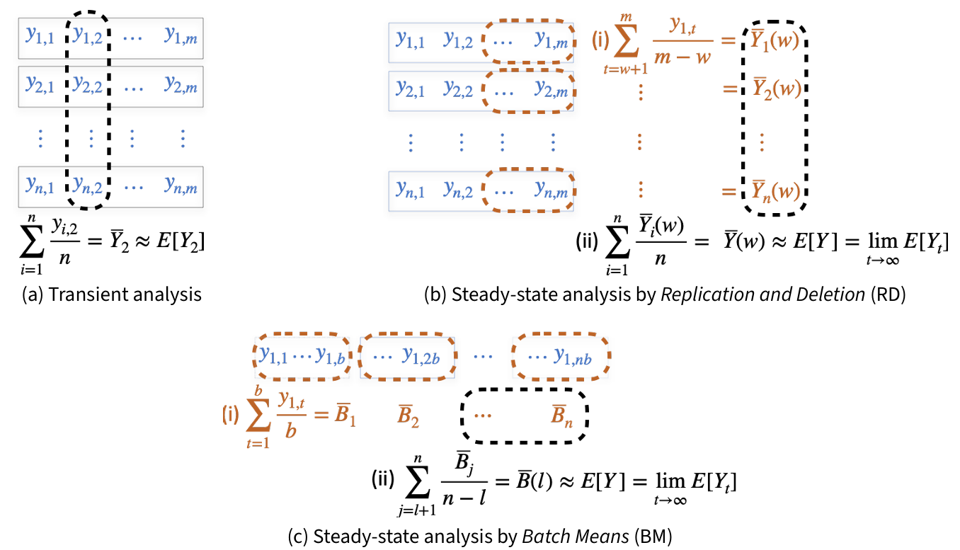
The analysis of ABMs often builds on stochastic simulations, based on Monte Carlo methods to estimate model characteristics (see e.g.,Fagiolo et al. 2019; Lee et al. 2015; Richiardi et al. 2006). In the majority of cases, we can think of (the output of) an ABM as a collection of discrete-time stochastic processes \((\mathbf{Y}_t)_{t>0}\) describing the evolution over time \(t\) of variables of interest (e.g., the wealth of an agent, the average population count of a category of agents, etc.). For clarity, consider the case in which \((\mathbf{Y}_t)_{t>0}\) contains only one time series of interest \((Y_t)_{t>0}\). That is, \(Y_t\), for each \(t>0\), is a random variable of interest defined over the ABM. Figure 1(a) provides a pictorial representation of \(n\) independent replications of a single variable \(Y_t\) (one per row) each comprising \(t=1,\ldots, m\) steps (one per column).⁵ The outcome of a simulation \(i\) can be represented as \(y_{i,1},\ldots,y_{i,m}\), a sequence of observations (or realizations) of length \(m\). The observations within the same column \(t\) are independent and identically distributed (IID), while those in the same row \(i\) are not.

As mentioned in the introduction, and as discussed in detail in (Vandin et al. 2022), MultiVeStA focuses on two typical classes of properties:

• Transient properties: the expected value of a property of a model at a given time \(t\) (or within a time range, or at the occurrence of a specific event); As depicted in Figure 1 (a), for a given point of interest \(t\) this can be expressed as \(E[Y_t]\).
• Steady-state properties: the expected value of a property of a model when it has reached a statistical equilibrium (i.e., at steady state). As depicted in Figure 1 (b), this can be expressed as \(E[Y]\!=\!\lim_{t\to\infty} E[Y_t]\).

Examples of transient properties are given in Section 3, where we study the average number of households alive for each of the 550 time points of interest for the artificial Anasazi model (Axtell et al. 2002; Dean et al. 2000). Here, a transient analysis is necessary because the model was proposed to replicate pointwise historical data, without any interest for steady states. In order to estimate such properties, MultiVeStA offers the method autoIR discussed later. Instead, an example of steady-state property can be found in Section 4. Here, we consider a typical ABM in ecology (Railsback & Grimm 2012) developed to study long-term survival ratios of birds species. Here, steady-state analyses are necessary because the modeler is interested in steady-state properties. Steady-state analyses require a statistical equilibrium; that is, \(\lim_{t\to\infty} E[Y_t]\) must exist and be finite. To automatically check when this assumption holds, Vandin et al. (2022) proposed a diagnostic. For the cases in which it holds, they proposed two steady-state methods, namely autoRD, based on the so-called Replication and Deletion (Figure 1 (b)), and autoBM, based on Batch Means (Figure 1 (c)). Both rely on an algorithm for estimating the end of the initial warmup period of the simulator, named autoWarmup. This is used by autoRD and autoBM to discard initial steps of simulation which are affected too much by the initial conditions, washing out the initial transient phase of the model. Then, the two approaches differentiate in that autoRD performs several short simulations, while autoBM performs a long simulation.

Algorithms such as autoRD are among the most common in the literature (see e.g., Fagiolo et al. 2019; Windrum et al. 2007). Social scientists typically study the statistical properties of a computational model by collecting a sufficiently large number of independent replications and discarding the initial steps of each run. However, as argued by (Alexopoulos & Seila 1996) and (Alexopoulos & Goldsman 2004), this methodology can be suboptimal when the model exhibits a long transient phase. In such cases, replication and deletion wastes substantial computational time generating observations that cannot be used for steady-state inference because they are affected by initialization bias. The batch means method addresses this issue by running a single, sufficiently long simulation, partitioning the output into non-overlapping windows (batches), and computing the average of the quantity of interest within each batch. The resulting batch means are then used to estimate the steady-state value and construct a confidence interval. The total run length (and, consequently, the batch size and number of batches) is crucial for reliability. In line with related approaches (e.g., ASAP3 by Steiger et al. 2005), autoBM automates this procedure by adaptively selecting run length and batching parameters while monitoring diagnostics such as low correlation and approximate normality of the batch means (see Vandin et al. 2022 for further detail). autoBM cannot fully replace autoRD. When the warmup period is relatively short and the available hardware supports a high degree of parallelization, replication and deletion is preferable. The appropriate method therefore depends on the model and computational environment. Moreover, the ergodicity diagnostic proposed by (Vandin et al. 2022) compares the results obtained with autoBM and autoRD.

MultiVeStA offers an intuitive property specification language, MultiQuaTEx. Using MultiQuaTEx, one can express both transient and steady-state properties. In the latter case, one can also just check for the end of the initial warmup period of the model, necessary for steady-state analysis.⁶

MultiQuaTEx for transient properties

A MultiQuaTEx query for transient analysis can describe one or more random variables evaluated on a model, each evaluated using the same simulations and with their own confidence interval (CI). Listing 1 depicts a MultiQuaTEx query used in Section 3 to study the evolution of (i) the number of households (line 5), and (ii) the difference between the simulated number of households and the historical data (line 6), in the first 570 simulation steps (line 7). Therefore, it considers 1140 random variables, meaning that each simulation will give one sample for each of the 1140 random variables. Following the discussion in Section 2 of (Vandin et al. 2022), the expected value of each random variable denoted by a MultiQuaTEx query is estimated as the mean \(\overline{Y}\) of \(n\) samples (coming from \(n\) independent replications), with \(n\) large enough but minimal to guarantee that the \((1-\alpha) \cdot 100\%\) CI centred on \(\overline{Y}\) has size at most \(\delta\), for given \(\alpha\) and \(\delta\).

The user provides MultiVeStA with a desired statistical significance level \(\alpha\) and interval width \(\delta\). MultiVeStA uses the method autoIR, which performs independent replications until each point estimate has a confidence interval of width at most \(\delta\), with statistical confidence \(1-\alpha\). It does so by performing an initial number \(n\) of replicas (user-specified, default 20), computes the mean value \(\overline{Y}_t\) at each time-step, and calculates the confidence interval as

\[\overline{Y}_t\pm \boldsymbol{t}_{n-1,1-\frac{\alpha}{2}}\sqrt{\frac{s^2_t}{n}}\,,\]

\[(1)\]

where \(\boldsymbol{t}_{n-1,1-{\alpha}/{2}}\) refers to the \(1-{\alpha}/{2}\) quantile of a Student-t distribution with \(n-1\) degrees of freedom and \(s^2_t\) is the unbiased estimator of the variance. If the width of the confidence interval, \(2\boldsymbol{t}_{n-1,1-{\alpha}/{2}}\sqrt{{s^2_t}/{n}}\), is smaller than \(\delta\) for some \(t\), then the corresponding estimates are stored, and those points are not considered anymore in future simulations. This means that, even if more simulations are run, the estimates for these points will ignore future samples. If for some \(t\), instead, the interval width is larger than \(\delta\), further \(n\) independent replicas are performed. The mean value and confidence interval computations are iteratively computed, considering each time \(n\) more simulations. At each iteration, more points may reach the required confidence interval width, and will therefore be ignored in future iterations. The algorithm keeps iterating by adding more independent replicas until all points have confidence intervals smaller than \(\delta\). When this happens, the results are shown (for further detail, see Vandin et al. 2022). The same simulations can support the independent estimation of multiple variables.

obsAtStep(step,obs) = if (s.eval("steps") == step)

then s.eval(obs)

else next(obsAtStep(step,obs))

fi ;

eval autoIR(E[ obsAtStep(step,"tothouseholds") ],

E[ obsAtStep(step,"abs(tothouseholds - histothouseholds)") ],

step,0,1,570) ;

The query starts with a list of parametric operators that can be used in an eval autoIR command to specify the properties to be estimated. Lines 1-4 of Listing 1 define the parametric operator obsAtStep having two parameters, step and obs, respectively the step and observation of interest. Lines 5-7 instantiate such operator for each of the 1140 random variables considered, allowing to obtain 1140 corresponding samples per simulation. In particular, 0 is the initial step to be considered, 1 is the increment to be iteratively added to it, and 570 is the final step to be considered. As shown in Lines 1-4, in the operator definition we may use s to denote the current simulation state, the function eval to evaluate expressions in s (e.g., the current number of performed steps and the observations obs specified in Lines 5-6, or expressions using NetLogo’s query languages), and the function next to ask the simulator to perform one step of simulation. An operator may contain:

1. conditional statements (the if-then-else-fi);
2. real-valued observations on the current simulation state (the s.eval in Line 1 and Line 2;
3. a next operator
4. arithmetic expressions.

In Listing 1, the operator checks whether the simulation has reached the step of interest (Line 1), in which case it returns the required observation (Line 2). Otherwise, it advances the simulation (Line 3) and recursively evaluates the operator in the next simulation state.

MultiQuaTEx for steady-state properties and warmup analysis

MultiQuaTEx also supports the steady-state and warmup analysis capabilities of MultiVeStA introduced in Vandin et al. (2022).

Listing 2 provides a steady-state MultiQuaTEx query used in Section 4 to study the average bird population and other steady-state properties. The count, with, and related commands shown in the query are primitive reporter procedures of NetLogo’s language that evaluate expressions on the current simulation state. The structure of the query is simpler than the one for transient analyses, as the progressing of simulation steps is performed implicitly in the analysis procedure. For this reason, we replace the operator obsAtStep with the simpler operator obs which just returns the observation of interest in the current simulation step. The query is then completed by one of the three types of supported steady-state analyses shown in Lines 3-5.

obs(o) = s.eval(o) ;

eval autoWarmup(E[obs("count turtles") ],

E[ obs("count patches with [count (turtles-here with [is-alpha?]) < 2]") ];

eval autoBM(E[obs("count turtles") ],...) ;

eval autoRD(E[obs("count turtles") ],...) ;

In particular, a steady-state query is composed of two parts:

1. A list of next-free operators,
2. one of the three eval commands in Listing 2, provided with a list of operators to consider.

autoWarmup performs the warmup estimation procedure from (Vandin et al. 2022) for each of the listed properties because different random variables may have different warmup periods. After estimating the warmup period for each property, autoBM and autoRD run the batch means or replication and deletion procedures from (Vandin et al. 2022) to estimate each property in the steady state, discarding the corresponding warmup periods. The estimates produced by autoBM and autoRD have \((\alpha,\delta)\) confidence intervals as for transient properties.

MultiQuaTEx supports two further eval commands: manualBM and manualRD. These behave similarly to autoBM and autoRD, but take the warmup length as an input, rather than estimating it. These commands are useful when this information is known. In Section 4 we use them to replicate analyses from the literature.

Transient Analysis and Calibration Application: Artificial Anasazi Model

We apply transient analysis to the “Artificial Anasazi” model originally proposed by Dean et al. (2000) and Axtell et al. (2002), and further explored by Janssen (2009). For all our applications, we use the NetLogo implementation provided by Stonedahl & Wilensky (2010).⁷ The model is meant to reproduce the dynamics of the Kayenta Anasazi population dwelling in the Long House Valley in the Black Mesa area of northeastern Arizona (U.S.) between 800 and 1350 AD. The ecological landscape of the Long House Valley – in particular, the annual fluctuations in potential agricultural production – is closely reconstructed using paleoenvironmental research data. Such a landscape is populated by artificial agents representing households that are initialized on nutritional requirements and demographic characteristics from ethnographic studies. Each household has agent-specific attributes (e.g., age, size, composition, amount of maize consumed, maximum amount of maize that can be stored, use of total potential maize yield) and interacts with others according to behavioral rules. The rules determine where the household should locate its maize plantation and dwelling. In each period \(t=800,\ldots,1350\), corresponding to a calendar year, every agent performs agricultural activities, harvests, consumes, and can change its plots and/or dwelling location based on whether its nutritional needs have been met. Moreover, the population evolves over time, since, depending on their nutritional success, households can reproduce or disappear. At the end of each period, the total number of households and their location are recorded, such that the artificial population dynamics can be compared with the real dynamics reconstructed using archaeological and environmental data.

In this setting, Axtell et al. (2002) show how, after calibrating its parameters, the model can closely reproduce key spatial and demographic features of the dynamics of Anasazi population. Janssen (2009) deepens the previous analysis focusing on the total number of households. The author considers five key parameters (death age, end of fertility age, fission probability, harvest adjustment, harvest variance) and shows that accurate calibration only partially contributes to the good fit of the model. Instead, the exogenously given carrying capacity (that is, the number of locations that have a yield equal or higher than the nutrition needs) is the fundamental driver of the success of the model in matching the data. Hence, harvest-related parameters appear to be more important than the demographic ones in explaining the model performance.

In establishing the fitness of each combination of parameter values, both Axtell et al. (2002) and Janssen (2009) use the same methodology. They perform 15 independent replications (simulations) with different random seeds. For each independent replication, they compute the average distance (over time) of the model-generated number of households from the empirical time series, using either the \(L^1\) or the \(L^2\) norm. Then, the smallest value of average distance, among the 15 computed, is assigned to the parameter combination as its fitness measure. The best parameter combination is selected as the one minimizing the fitness measure over the set of combinations considered. In showing the results, Axtell et al. (2002) argue that: “the average run, produced by averaging over 15 distinct runs, looks quite similar” (to the one they show relative to the best parameter combination). Similarly, after simulating the model 100 times using the best combination from Axtell et al. (2002), Janssen (2009) reports “some variation in the results”.

The outcomes of the Artificial Anasazi model, similarly to those of the vast majority of agent-based models, can be profoundly affected by the intrinsic stochasticity deriving from the sequence of random draws characterizing its functioning. As a consequence, any measure of fitness that is attached to a parameter combination on the basis of a given number of independent replications is itself a random variable. Hence, it suffers from estimation errors that need to be quantified and assessed when making decisions such as choosing the best parameter combination. Any assessment of concordance between real and simulated data should therefore account for simulation variability. Neither Axtell et al. (2002) nor Janssen (2009) deal with these potential problems in their calibration exercises and concordance assessments. We therefore conduct two analyses: a transient analysis of the parameterization identified by Janssen (2009), followed by a calibration exercise that controls estimation uncertainty.

Transient analysis of the best parameter combination by Janssen (2009)

The first analysis estimates the total number of households for each \(t=800,\ldots,1350\). In Figure 2, we present the outcomes of our analysis under the best combination of parameters by Janssen (2009).

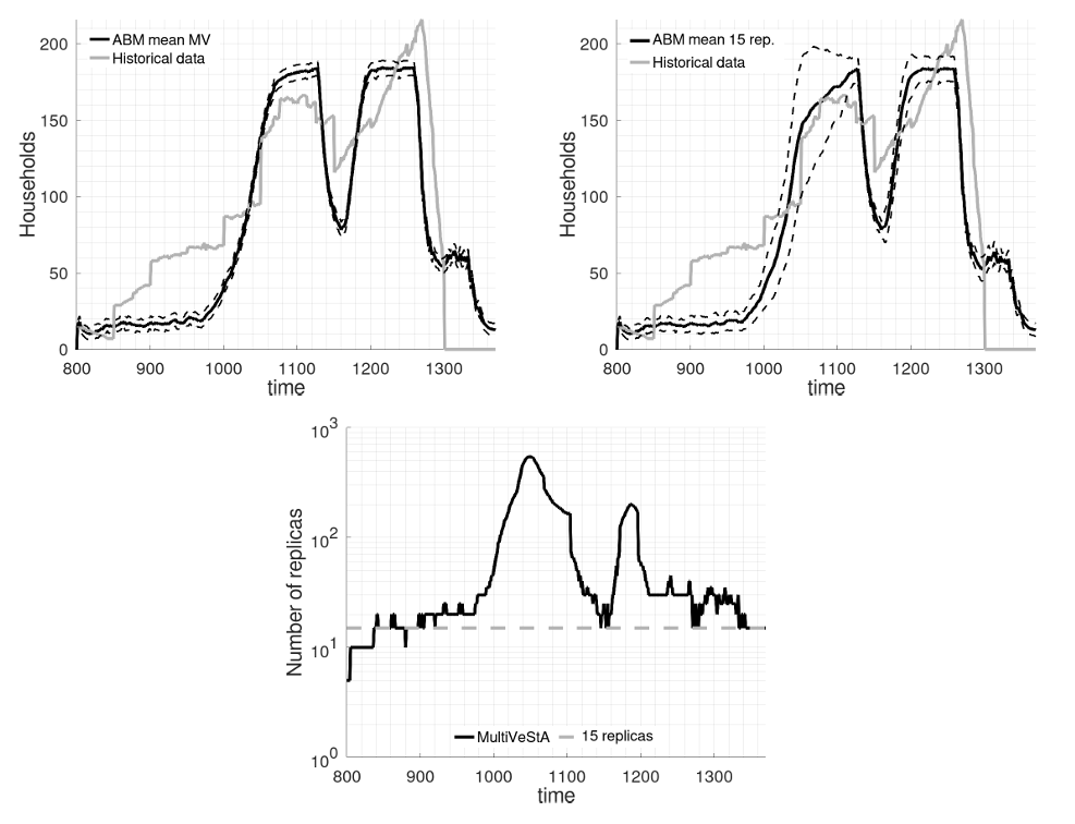
In the top-left panel we present the results of the transient analysis obtained setting significance level \(\alpha=0.01\) and width of the confidence interval \(\delta=10\), and the real historical data. The resulting point estimates roughly resemble the single run shown by Janssen (2009) in Figure 10. They show an initial stationary phase, followed by a steep increase around time \(1000\). Then, the number of households stabilizes until time \(\sim1120\), when a sharp decrease in population occurs. The number of households recovers around time 1200 and remains constant until time \(\sim1260\), when the population rapidly decreases until the final collapse. Such a similarity may indicate that the variability under the proposed parameter settings is quite low.

To improve the comparison, in the top-right panel we perform the same estimation exercise fixing the total number of independent replicas for each time step to 15, matching the sample size used by Janssen (2009). The plots generally agree. However, between 1050 and 1150, the estimates obtained with 15 independent replicas have particularly wide confidence intervals and differ substantively from those in the top-left panel. This may cause erroneous statements in assessing model performance. For instance, from the 15-replication exercise one may conclude that in the interval 1050–1150 the model’s average number of households is not statistically different from the historical data because the historical data lie within the wide confidence intervals. This is an artifact of the low number of independent replicas fixed in advance. As shown in the top-left panel, the statement becomes false after refining the estimates for that period with more independent replications. The bottom panel presents the number of independent replicas that MultiVeStA performed for the transient analysis at each time point. For the 1050–1150 interval, this number is between 100 and 600. Conversely, fewer than 20 runs are sufficient during the first 100 periods.

In summary, MultiVeStA’s transient analysis efficiently and reliably estimates the average number of households in each time step, avoiding conclusions based on an insufficient number of replicas. The next analysis applies the same method to calibration with statistical guarantees.

Model calibration with statistical guarantees

In the previous application we simply requested MultiVeStA to estimate the mean and the confidence interval of a given variable of interest at all \(t\). However, MultiVeStA allows the user to estimate mean and confidence interval of a given function of the variable of interest recorded at any interval of time. This can be used to perform a new application of the transient analysis: calibrating the model with statistical guarantees.

For a parameter combination \(\theta\) and random-number seed \(i\), define the loss as

\[\mathcal{L}_i(\theta)=\sum\limits_{t=800}^{1350} \left|\hat{h}_{i,t}(\theta)-h_t\right|\,\]

\[(2)\]

where \(\hat{h}_{i,t}(\theta)\) is the total number of households generated by the model at time \(t\) with seed \(i\) and \(h_t\) is the historically recorded number of households at the same date. Notice that this quantity is actually the same one that Axtell et al. (2002) and Janssen (2009) use to evaluate a single trajectory under the \(L^1\) norm multiplied by a factor of 550 (the total number of steps). We estimate the loss while controlling the stochastic variability induced by the random seed. As in the previous subsection, we use the arithmetic average across \(n\) independent replications, where \(n\) is selected so that the estimate has a confidence interval of width \(\delta\) with statistical confidence \(1-\alpha\):

\[\overline{\mathcal{L}}(\theta;\alpha,\delta)=\sum\limits_{i\in\mathcal{I}(\theta;\alpha,\delta)} \frac{\mathcal{L}_i(\theta)}{|\mathcal{I}(\theta;\alpha,\delta)|}\,,\]

\[(3)\]

where \(\mathcal{I}(\theta;\alpha,\delta)\) is a set of seeds with cardinality \(|\mathcal{I}(\theta;\alpha,\delta)|\) such that the confidence interval of \(\overline{\mathcal{L}}(\theta;\alpha,\delta)\) with statistical significance \(\alpha\) has width at most \(\delta\). Hence, we can use the previously described transient analysis, the only change we have to make is that now MultiVeStA should evaluate the variable of interest (the loss) only at \(t=1350\). This can be easily done by asking MultiVeStA through its query system to compute the absolute difference between artificial and historical data at any \(t\), store its cumulative sum, and statistically evaluate the cumulative sum only at the final time period. In other words, the query language of MultiVeStA is expressive enough to state those properties. Notice that all these steps can be done without changing anything in the model’s code, simply querying MultiVeStA.

The procedure just described is repeated for any combination of the parameters reported in Table 1, with the caveat of discarding those combinations where end of fertility age is larger than death age. We run the MultiVeStA transient analysis for all the 1600 parameter combinations setting \(\alpha=0.1\) and \(\delta=1000\). Then, the minimization principle used by Axtell et al. (2002) and Janssen (2009) would suggest selecting the combination with the lowest loss. However, the estimated values are subject to estimation error. To account for this uncertainty, we take the minimum estimated loss as a reference point and discard all parameter combinations whose estimated loss is significantly larger than the minimum according to Welch’s t-test (Welch 1947) for difference of means with \(1-\alpha\) confidence level, \(90\%\) in our case (we used \(\alpha=0.1\)). The remaining parameter combinations cannot be considered significantly different from the one with the lowest estimated loss; they are shown, together with technical details provided by MultiVeStA and the p-value of the Welch’s t-test, in Table 2. The combination with the lowest estimated loss is \(\{38,38,0.135,0.56,0.4\}\) (in blue in the table). It does not coincide with the one identified by Janssen (2009) (in red in the table). This aligns with our argument regarding the statistical error associated with estimating loss: given a certain confidence level and estimation precision, there may be parameter combinations whose differences in loss are not statistically significant. Discarding these to focus solely on a single combination may therefore be misleading and result in information loss. For example, identifying patterns within the set of parameter configurations that are not significantly different from the minimum-loss combination can provide insights into the relative importance of different parameters in replicating real data.

Table 1: Parameter values considered.

Parameter	Values
Death Age	\(\{26,30,34,38\}\)
End of Fertility Age	\(\{26,30,34,38\}\)
Fission Probability	\(\{0.095,0.105,0.115,0.125,0.135,0.145,0.155,0.165,0.175,0.185\}\)
Harvest Adjustment	\(\{0.54,0.56,0.58,0.6\}\)
Harvest Variance	\(\{0,0.2,0.4,0.6\}\)

The values reported in Table 2 support the argument made by Janssen (2009) regarding the relatively greater importance of harvest-related variables compared to demographic ones in replicating historical population data. All the statistically indistinguishable parameter combinations include a harvest adjustment of 0.56 and a harvest variance of 0.4, while the other parameters exhibit some variation. This suggests that harvest-related parameters must take specific values for the model to closely match historical data, whereas demographic parameters appear to be less critical.

Table 2: Parameter combinations not statistically distinguishable from the minimum-loss combination, with values of death age (DA), end of fertility age (EFA), harvest adjustment (HA), and harvest variance (HV), together with the estimated loss, confidence-interval width, estimated loss variance, and number of runs used by MultiVeStA to meet the requirements \(\alpha=0.1\) and \(\delta=1000\). In red, the best parameterization according to Janssen (2009); in blue, the combination with the lowest estimated loss under our approach.

Parameters					Obtained measures
DA	EFA	FP	HA	HV	Estim. Loss	Width C.I.	Estim. Var.	Runs	p-value
34	30	0.185	0.56	0.4	18002	783.35	1707620	32	0.7285
34	34	0.145	0.56	0.4	18432	973.80	12455019	144	0.1461
34	34	0.165	0.56	0.4	18215	847.01	1996478	32	0.3376
34	34	0.175	0.56	0.4	17926	817.76	870417	16	0.9106
34	34	0.185	0.56	0.4	18265	649.56	1174162	32	0.2109
38	30	0.185	0.56	0.4	18121	807.07	2776238	48	0.4859
38	34	0.155	0.56	0.4	17923	817.87	2851035	48	0.9191
38	34	0.165	0.56	0.4	18467	970.53	2621220	32	0.1192
38	34	0.175	0.56	0.4	18335	886.03	2184662	32	0.2023
38	34	0.185	0.56	0.4	18232	983.16	1258101	16	0.3481
38	38	0.135	0.56	0.4	17889	771.83	1657766	32	1.0000
38	38	0.145	0.56	0.4	18409	951.02	14553463	176	0.1577
38	38	0.155	0.56	0.4	18175	940.52	2461623	32	0.4287
38	38	0.175	0.56	0.4	18373	938.87	1147316	16	0.1768

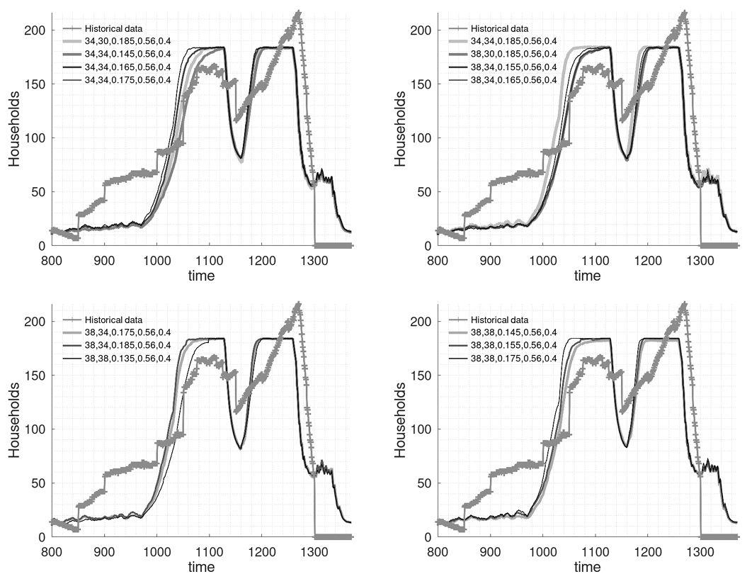
In Figure 3, we present the time series of the mean number of households resulting from the 14 parameter combinations listed in Table 2. One can observe that the trajectories are remarkably close at each time step. The largest differences appear between the years 1000 and 1100, a period already identified in previous analyses as one where the model exhibits greater volatility.⁸

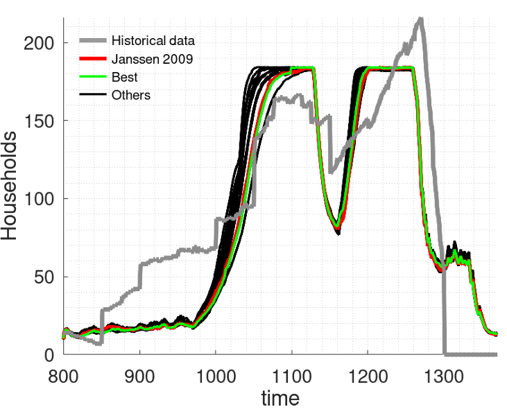
The calibration procedure with statistical guarantees, as performed here using MultiVeStA’s transient analysis, can be refined by reducing \(\alpha\) and \(\delta\). Doing so narrows the set of statistically indistinguishable parameter combinations, thereby increasing the precision of the results. However, this refinement also requires greater computational resources, whether in terms of processing power or time. To address this trade-off, we propose a sequential approach: start with relatively large values of \(\alpha\) and \(\delta\), then iteratively reduce them—applying each refinement to the resulting subset of candidate combinations—until either a single combination is identified or the maximum resource allocation is reached. This method allows for a meaningful balance between accuracy and computational cost in the calibration process.

Notice that our calibration procedure is likelihood-free in the sense that it relies on repeated simulations of the model and a function measuring the discrepancy between simulated and observed data. In this respect it is related to Approximate Bayesian Computation (ABC; see e.g., Grazzini et al. 2017; Lux 2023, for applications to the calibration of agent-based models), which approximates the posterior distribution of parameters by sampling from a prior and retaining (or weighting) parameter values that generate simulations sufficiently close to the observations under a tolerance (Sisson et al. 2018). However, the goal and interpretation differ: we adopt a frequentist perspective and use repeated seeds to estimate the expected loss with a prescribed precision, subsequently identifying a set of parameter vectors that are not statistically distinguishable from the minimum-loss combination. Thus, we obtain a confidence-set-style output rather than a posterior over \(\theta\).

By leveraging MultiVeStA’s transient analysis, we evaluated a comprehensive set of parameter combinations, explicitly accounting for the uncertainty in loss estimation. Rather than selecting a single “best” configuration, our procedure identifies a set of statistically indistinguishable parameter combinations. This is in line with the philosophy of the Model Confidence Set approach proposed by Hansen et al. (2011) and recently applied to model calibration by Seri et al. (2021). Indeed, our method acknowledges that, given estimation uncertainty, multiple specifications may perform equivalently well, and that prematurely narrowing the choice may lead to information loss. This perspective not only highlights the relative importance of certain parameters (such as the dominant role of harvest-related variables in the Artificial Anasazi model) but also enables an iterative and resource-aware refinement of the calibration process.

Warmup and Steady State Analysis: Alpha Birds Model

We evaluate MultiVeStA’s steady-state analysis by determining (i) the required number of independent replications and (ii) the duration of the warm-up and post-warm-up simulation.

To exemplify MultiVeStA’s capabilities, we consider the “Alpha birds” model, which is an ABM of a territorial bird species whose long-term survival crucially depends on its reproductive characteristics (Railsback & Grimm 2012). This model has several advantages. On one hand, it is a typical ABM in ecology, featuring a simplified representation of population dynamics and social behaviors. On the other hand, its steady state features, as will be clarified below, make it an ideal test case for our tools that automatically determine if the steady state has been reached. In addition, this model has already been used by Thiele et al. (2014) to illustrate the features of the RNetLogo package, suggesting that it is a good baseline model that can be approached by various techniques. Interestingly, in the Discussion section of Thiele et al. (2014), the authors raise the issue that it is often unclear how many independent replications are needed to reliably estimate model properties. They say that: "Very likely, just 10 iterations, as used here, will often not be enough". As explained in Section 2, this is one of the issues addressed by both our transient and steady state analyses.

The model represents a territorial bird species that lives in groups and exhibits reproductive suppression. The alpha pair in each group suppresses the reproduction of subordinate mature birds. Subordinate birds may leave their territory on scouting forays to search for available alpha positions, but these forays increase their risk of mortality due to raptors.

As in Thiele et al. (2014), we use the simplest model version, in which the probability that a subordinate undertakes a scouting foray is constant.

Thus, a crucial parameter of the model is the scouting probability. There is another important parameter, which is the overall survival probability of any bird. Thiele et al. (2014) explore the response of the model to variations in these two parameters. They focus on three key quantities as key outputs:

• Abundance, i.e., the total number of birds in all territories;
• Variation, i.e., the standard deviation of the total number of birds over time;
• Vacancy, i.e., the fraction of territories with at least one vacant alpha bird.

In their main exercise, the authors explore survival probabilities between 95% and 100% and scouting probabilities between 0% and 50%. They consider the mean of the three key outputs across 10 independent replications and run the model for 264 monthly time steps (22 years). The authors discard the first two years and then measure Abundance, Variation and Vacancy every 12 months, at time steps 35, 47, 59, \(\dots\), 263.

We replicate the calibration experiments of Thiele et al. (2014) after testing whether 10 independent replications and a two-year warm-up are sufficient.

Number of independent replications

We replicate the analysis of Thiele et al. (2014) using the manualRD feature of MultiVeStA, obtaining the values of Abundance, Variation and Vacancy at time steps 35, 47, 59, \(\dots\), 263. MultiVeStA estimates are equipped with confidence intervals. We set maximum confidence-interval widths of \(\delta=5\) for Abundance, \(\delta=1\) for Variation, and \(\delta=0.04\) for Vacancy. The values differ because the three variables have different orders of magnitude and are approximately 10% of the median of each variable.

As discussed, confidence intervals are computed iteratively by performing blocks of \(n\) independent replications. Here we set \(n=10\). In this way, the minimum number of replications is 10, as in Thiele et al. (2014). If 10 replications are not enough for a property, 10 more replications will be performed, and we proceed this way until we identify the minimal amount of independent replications that are needed to obtain statistically valid results with confidence intervals respecting the required \(\delta\).

Figure 4 shows how many independent replications are needed to estimate Abundance, Variation and Vacancy for each of the 121 parameterizations. For survival probabilities close to the extremes of the considered interval (around 95% and 100%), the 10 independent replications considered by Thiele et al. (2014) are typically sufficient. For intermediate survival probabilities between 97% and 97.5%, many more simulations are required. For instance, with survival probability 97% and scouting probability 25%, statistically valid results require 90 replications for Abundance, 100 for Variation, and 110 for Vacancy. When scouting probability is zero, many replications are required for survival probabilities between 97% and 99%; at 99% survival probability, 350 replications are required for Variation.

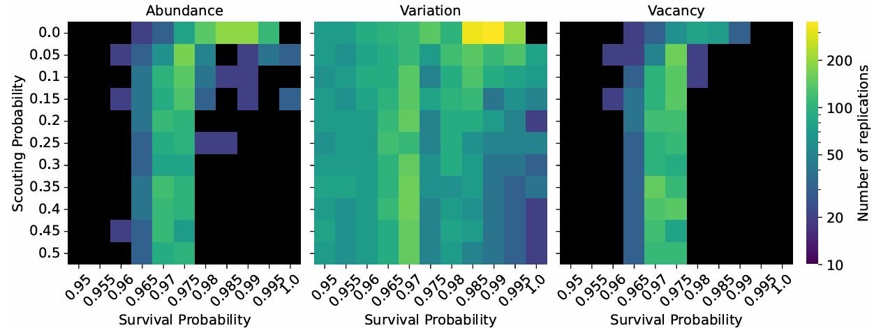
This exercise demonstrates that, for many parameter combinations, running 10 simulations for each property for each parametrization as done in Thiele et al. (2014) is not enough to obtain statistically reliable estimations.

To understand why many more independent replications are needed in certain parts of the parameter space, in Figure 5 we plot the values of Abundance, Variation and Vacancy for all the combinations of parameter values in Figure 4. We plot these values both when considering only 10 replications (left), as in Thiele et al. (2014), and when considering \(N\) independent replications (right), as automatically determined by MultiVeStA.

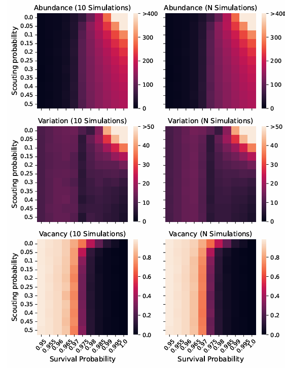
For 10 replications (left column), Abundance is close to zero for survival probabilities below 97%, suggesting that the bird population tends toward extinction. Abundance reaches higher values, up to 400 birds, for higher survival probabilities, especially in combination with low scouting probability. Vacancy shows the opposite pattern because high Abundance implies few vacant territories. Variation is highest where Abundance is highest but lowest at a survival probability of 97.5%, where Abundance and Vacancy change substantially. Overall, the region requiring the most replications coincides with transitions in the key metrics.

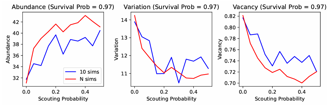
The results for 10 and \(N\) independent replications are qualitatively similar, but Variation and Vacancy are noisier with 10 replications. For survival probabilities of 96.5% and 97%, there are sizable fluctuations across scouting probabilities with 10 replications, whereas the results are more consistent with \(N\) replications (Figure 6). Thus, an appropriate replication count yields smoother estimates of model output across parameter values.

To check the implications of our results, we replicate the first experiment performed in Thiele et al. (2014). The authors were interested in showcasing some calibration methods and, as a first approach, tested a full factorial design with the 121 parameter combinations that we have been considering. In this design, acceptable values for model outputs were between 115 and 135 for Abundance, 10 and 15 for Variation, and 0.15 and 0.30 for Vacancy. The idea was to check if any parameter combinations would make the model produce an output that was within all three ranges. If taken to characterize a real-world ecosystem, this calibration procedure would find under which parameters the model best describes empirical data. The key result was that no parameter combination fulfilled all three requirements.

The left panel of Figure 7 replicates the calibration results in Thiele et al. (2014). There are small differences due to different random seeds, but the overall patterns are similar. The right panel shows the results when MultiVeStA determines the number of independent replications. For instance, green crosses appear for eight parameter combinations when scouting probability is 97.5%, compared with four when using 10 simulations. At 98% survival probability, Variation lies between 10 and 15 for four scouting-probability values under 10 replications and for two values under \(N\) replications. With \(N\) replications, no two conditions are satisfied simultaneously; with 10 replications, this occurs for three scouting probabilities when survival probability is 98%.

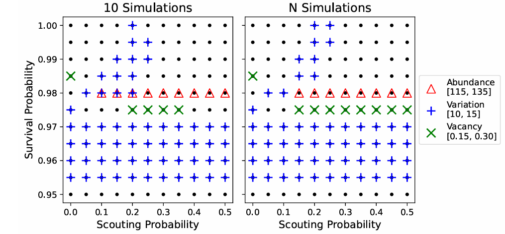
We confirm the main result in Thiele et al. (2014): no parameter combination satisfies all three requirements simultaneously. However, statistically reliable estimates are particularly important in transition regions of the parameter space.

Warmup analysis

Thiele et al. (2014) discard an initial two-year warm-up. We use MultiVeStA to test whether this period is sufficient for the model to reach steady state.⁹

Figure 8 focuses on Abundance and Vacancy for all survival probabilities and three selected scouting probabilities.¹⁰ Each panel compares manualRD (also shown in Figure 5) with autoRD, which tests whether steady state has been reached.

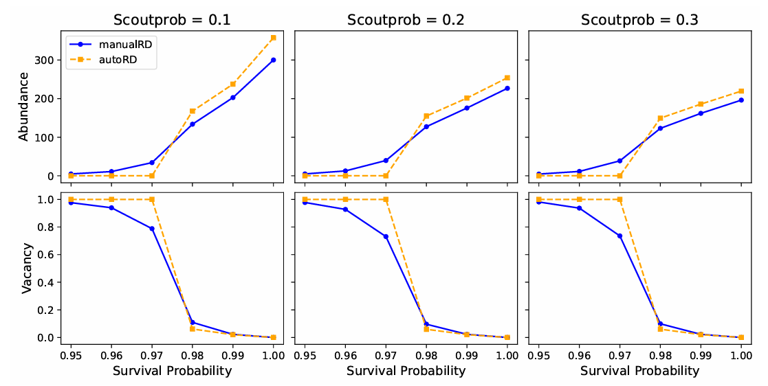
Our key result is that, for autoRD there is a sharp transition in Abundance and Vacancy at survival probability equal to 0.97. When survival probability is smaller than 0.97, they take value 0 and 1, respectively, but when survival probability is larger than 0.97, Abundance takes positive value and Vacancy is close to 0. By contrast, for manualRD the transition is much smoother.

This suggests that the smooth transitions that can also be seen in Figure 5 are really driven by warm-ups. However, in the long run, either the bird species survives, or it collapses.

Discussion

This paper makes complementary technical and methodological contributions. The technical contribution is the integration of MultiVeStA, a statistical model checking framework, with NetLogo, a widely used ABM platform. The methodological contribution is the extension of transient analysis to calibration through statistical comparisons among candidate parameterizations.

The integration provides NetLogo users with automated statistical tools that can determine the number of simulations, the length of warm-up periods, and the appropriate duration of steady-state runs with statistical guarantees. It builds on Thiele et al. (2014), Thiele (2014) and (Vandin et al. 2022) by supporting reproducible, quantitative evaluations of model behavior within NetLogo. The integration reduces reliance on ad hoc rules of thumb. Although it requires some familiarity with property specification and statistical settings, it reduces the effort needed to implement statistically sound analyses.

We evaluate the integration in two applications: one uses MultiVeStA’s transient analysis, and the other uses its steady-state analysis.

By applying the transient analysis techniques to the calibration of the Artificial Anasazi model, we demonstrated that widely used calibration strategies based on a small fixed number of replications may lead to inaccurate conclusions. MultiVeStA’s adaptive allocation of simulations provided a richer picture, showing that several parameter combinations can be statistically indistinguishable in their ability to reproduce historical data. This finding reinforces the importance of acknowledging uncertainty in calibration exercises and cautions against the search for a single “best” parameter set. The method also confirmed the central role of harvest-related parameters in shaping population dynamics, thereby giving stronger statistical support to earlier (more qualitative) observations.

In the case of the Alpha Birds model, MultiVeStA identified limitations in previous analysis practices. The assumption of a fixed two-year warm-up period used in earlier studies was shown to be insufficient to capture critical transitions in population dynamics. Our results revealed sharp shifts in model behavior near parameter thresholds that would have been obscured without statistically guided warm-up and steady-state analysis. Moreover, the number of required replications varies substantially across regions of the parameter space, underscoring the risks of uniform rules of thumb for simulation design.

Several limitations remain. The computational burden of large-scale analyses is non-trivial, and although MultiVeStA supports parallelization, scaling to highly complex or computationally intensive models may pose challenges. While the integration is seamless at the technical level, non-expert users may still face a learning curve in specifying properties and interpreting statistical outputs. The statistical guarantees are conditional on the selected observables and statistical settings and do not validate the model structure or its substantive assumptions. Warm-up and steady-state analyses also require a relevant stationary regime to exist and be detectable; non-ergodic or rare-event dynamics may prevent convergence or require very long runs. Finally, the calibration results are conditional on the explored parameter space, loss function, and comparison procedure, so statistically indistinguishable parameterizations should not be interpreted as equivalent or globally optimal. Broader adoption will likely depend on developing more intuitive interfaces and community best practices.

Future research should therefore proceed along several directions. First, an important challenge is to extend the framework to cases of non-ergodicity, where models do not converge to a single stationary distribution and standard steady-state assumptions fail. Many social and economic ABMs exhibit path dependence, multiple equilibria, or lock-in effects, and developing tools to statistically analyze such dynamics would greatly expand the scope of rigorous ABM evaluation. Second, it would be interesting to investigate recent statistical model checking techniques that go beyond means (Budde et al. 2025) by allowing to estimate higher-order moments, quantiles and more. Third, efforts should focus on the efficient analysis of large-scale models, where the number of agents, parameters, or required simulations is substantial. Techniques such as adaptive sampling and surrogate modeling could help balance statistical reliability with computational feasibility, making it possible to apply our approach to models used for real-world policy or large-scale ecological management. Finally, another important avenue concerns advancing calibration and validation practices. While this paper has shown that leveraging MultiVeStA’s transient analysis one can identify sets of statistically indistinguishable parameter combinations, future work should build systematic workflows for calibrating models against empirical data and validating their predictions under uncertainty.

A further limitation concerns the software itself. MultiVeStA is distributed as a closed-source binary rather than as open-source code. As briefly mentioned in Section 2, this is not a deliberate choice: MultiVeStA extends PVeStA (AlTurki & Meseguer 2011) and, in turn, VeStA (Sen et al. 2005), whose licenses do not permit us to release the source code. As a consequence, users cannot directly inspect, modify, or extend its internal implementation. For the same reason, the tool does not currently provide the version-controlled source, unit tests, and continuous integration that are increasingly expected of research software. We acknowledge that this places part of the burden of trust on the user, however, we mitigate it in three ways. First, the algorithms implemented in MultiVeStA are described in detail in peer-reviewed publications (Sebastio & Vandin 2013; Vandin et al. 2022), so that they can be scrutinized and, if needed, reimplemented independently. Second, we now provide an explicit license and a permanently archived replication package for this paper on Zenodo (Vandin et al. 2026), together with installation instructions. Third, the tool has been actively developed since 2012, and we intend to continue maintaining it. In the future, we plan to fully overcome those issues by reimplementing the tool from scratch.

In conclusion, the integration of MultiVeStA with NetLogo combines a technical contribution with a methodological extension to calibration. Together, the two applications show that statistically checked analyses can reveal non-unique calibrated solutions and discontinuities in model dynamics. Making these procedures available within a widely used modeling environment can support more transparent and reproducible ABM studies.

References

AGHA, G., & Palmskog, K. (2018). A survey of statistical model checking. ACM Transactions on Modeling and Computer Simulation (TOMACS), 28(1), 1–39. [doi:10.1145/3158668]

ALEXOPOULOS, C., & Goldsman, D. (2004). To batch or not to batch? ACM Transactions on Modeling and Computer Simulation (TOMACS), 14(1), 76–114. [doi:10.1145/974734.974738]

ALEXOPOULOS, C., & Seila, A. F. (1996). Implementing the batch means method in simulation experiments. Proceedings of the 28th Conference on Winter Simulation, 214–221. [doi:10.1145/256562.256608]

ALTURKI, M., & Meseguer, J. (2011). PVESTA: A parallel statistical model checking and quantitative analysis tool. Proceedings of the 4th International Conference on Algebra and Coalgebra in Computer Science, CALCO'11, (pp. 386-392). Berlin, Heidelberg: Springer. [doi:10.1007/978-3-642-22944-2_28]

AXTELL, R. L., Epstein, J. M., Dean, J. S., Gumerman, G. J., Swedlund, A. C., Harburger, J., Chakravarty, S., Hammond, R., Parker, J., & Parker, M. (2002). Population growth and collapse in a multiagent model of the Kayenta Anasazi in Long House Valley. Proceedings of the National Academy of Sciences, 99(suppl 3), 7275–7279. [doi:10.1073/pnas.092080799]

BARTOLETTI, M., Chiang, J. H.-y., Junttila, T. A., Lluch-Lafuente, A., Mirelli, M., & Vandin, A. (2022). Formal analysis of lending pools in decentralized finance. In ISoLA 2022, Vol. 13703 of Lecture Notes in Computer Science (pp. 335–355). Springer. [doi:10.1007/978-3-031-19759-8_21]

BELZNER, L., De Nicola, R., Vandin, A., & Wirsing, M. (2014). Reasoning (on) service component ensembles in rewriting logic. In Specification, Algebra, and Software, Vol. 8373 of Lecture Notes in Computer Science (pp. 188–211). Springer. [doi:10.1007/978-3-642-54624-2_10]

BLANDO, S., Fagiolo, G., Giachini, D., Vandin, A., & Ivanaj, E. (2026a). Statistical model checking of the island model: An established economic agent-based model of endogenous growth. In M. H. ter Beek & G. Gössler (Eds.), Proceedings of the 7th workshop on models for formal analysis of real systems, MARS 2026, Turin, Italy, 12th april 2026 (Vol. 443 of EPTCS, pp. 3–22). [doi:10.4204/eptcs.443.2]

BLANDO, S., Guerrazzi, E., Porcedda, R., Squillace, G., Tschaikowski, M., & Vandin, A. (2026b). Towards agentic agent-based models: Feasibility, performance, and statistical model checking. CoRR, abs/2607.17948. http://arxiv.org/abs/2607.17948 [doi:10.1007/978-3-032-40121-2_13]

BRUNI, R., Corradini, A., Gadducci, F., Lluch-Lafuente, A., & Vandin, A. (2015). Modelling and analyzing adaptive self-assembly strategies with maude. Science of Computer Programming, 99, 75–94. [doi:10.1016/j.scico.2013.11.043]

BUDDE, C. E., Hartmanns, A., Meggendorfer, T., Weininger, M., & Wienhöft, P. (2025). Statistical model checking beyond means: Quantiles, cvar, and the dkw inequality. In P. Prabhakar & A. Vandin (Eds.), Quantitative evaluation of systems and formal modeling and analysis of timed systems - first international joint conference, QEST+FORMATS 2025, aarhus, denmark, 2025, proceedings. Springer. [doi:10.1007/978-3-032-05792-1_5]

CAIANI, A., Russo, A., & Gallegati, M. (2019). Does inequality hamper innovation and growth? An AB-SFC analysis. Journal of Evolutionary Economics, 29(1), 177–228. [doi:10.1007/s00191-018-0554-8]

CASALUCE, R., Burattin, A., Chiaromonte, F., & Vandin, A. (2023). Process mining meets statistical model checking: Towards a novel approach to model validation and enhancement. In C. Cabanillas, N. F. Garmann-Johnsen, & A. Koschmider (Eds.), Business Process Management Workshops (pp. 243–256). Cham: Springer International Publishing. [doi:10.1007/978-3-031-25383-6_18]

CASALUCE, R., Tschaikowski, M., & Vandin, A. (2024). White-box validation of collective adaptive systems by statistical model checking and process mining. In ISoLA 2024, Vol. 15219 of Lecture Notes in Computer Science (pp. 204–222). Springer. [doi:10.1007/978-3-031-73709-1_13]

CIANCIA, V., Latella, D., Massink, M., Paskauskas, R., & Vandin, A. (2016). A tool-chain for statistical spatio-temporal model checking of bike sharing systems. In ISoLA 2016, Vol. 9952 of Lecture Notes in Computer Science (pp. 657–673). [doi:10.1007/978-3-319-47166-2_46]

CORRADINI, F., Fornari, F., Polini, A., Re, B., Tiezzi, F., & Vandin, A. (2021). A formal approach for the analysis of bpmn collaboration models. Journal of Systems and Software, 180, 111007. [doi:10.1016/j.jss.2021.111007]

DEAN, J. S., Gumerman, G. J., Epstein, J. M., Axtell, R. L., Swedlund, A. C., Parker, M. T., & McCarroll, S. (2000). Understanding anasazi culture change through agent-based modeling. In T. A. Kohler & G. J. Gumerman (Eds.), Dynamics in Human and Primate Societies: Agent-based Modeling of Social and Spatial Processes (pp. 179–205). Oxford: Oxford University Press. [doi:10.1093/oso/9780195131673.003.0013]

FAGIOLO, G., Guerini, M., Lamperti, F., Moneta, A., & Roventini, A. (2019). Validation of agent-based models in economics and finance. In C. Beisbart & N. J. Saam (Eds.), Computer Simulation Validation (pp. 763–787). Berlin Heidelberg: Springer. [doi:10.1007/978-3-319-70766-2_31]

GALÁN, J. M., & Izquierdo, L. R. (2005). Appearances can be deceiving: Lessons learned re-implementing Axelrod’s ’evolutionary approach to norms’. Journal of Artificial Societies and Social Simulation, 8(3), 2.

GALPIN, V., Georgoulas, A., Loreti, M., & Vandin, A. (2018). Statistical analysis of carma models: An advanced tutorial. In Winter Simulation Conference (WSC 2018) (pp. 395–409). IEEE. [doi:10.1109/wsc.2018.8632456]

GILMORE, S., Reijsbergen, D., & Vandin, A. (2017). Transient and steady-state statistical analysis for discrete event simulators. In IFM (pp. 145–160). Springer. [doi:10.1007/978-3-319-66845-1_10]

GILMORE, S., Tribastone, M., & Vandin, A. (2014). An analysis pathway for the quantitative evaluation of public transport systems. In Integrated Formal Methods (IFM 2014), Vol. 8739 of Lecture Notes in Computer Science (pp. 71–86). Springer. [doi:10.1007/978-3-319-10181-1_5]

GRAZZINI, J., Richiardi, M. G., & Tsionas, M. (2017). Bayesian estimation of agent-based models. Journal of Economic Dynamics and Control, 77, 26–47. [doi:10.1016/j.jedc.2017.01.014]

HANSEN, P. R., Lunde, A., & Nason, J. M. (2011). The model confidence set. Econometrica, 79(2), 453–497.

JANSSEN, M. A. (2009). Understanding Artificial Anasazi. Journal of Artificial Societies and Social Simulation, 12(4), 13.

KETS, W., Pennock, D. M., Sethi, R., & Shah, N. (2014). Betting strategies, market selection, and the wisdom of crowds. Twenty-Eighth AAAI Conference on Artificial Intelligence. [doi:10.1609/aaai.v28i1.8808]

LEE, J. S., Filatova, T., Ligmann-Zielinska, A., Hassani-Mahmooei, B., Stonedahl, F., Lorscheid, I., Voinov, A., Polhill, G., Sun, Z., & Parker, D. C. (2015). The complexities of agent-based modeling output analysis. Journal of Artificial Societies and Social Simulation, 18(4), 4. [doi:10.18564/jasss.2897]

LEGAY, A., Lukina, A., Traonouez, L., Yang, J., Smolka, S. A., & Grosu, R. (2019). Statistical Model Checking. In B. Steffen & G. J. Woeginger (Eds.), Computing and Software Science: State of the Art and Perspectives (Vol. 10000 of LNCS, pp. 478–504). Springer. [doi:10.1007/978-3-319-91908-9_23]

LUX, T. (2023). Approximate Bayesian inference for agent-based models in economics: A case study. Studies in Nonlinear Dynamics & Econometrics, 27(4), 423–447. [doi:10.1515/snde-2021-0052]

PIANINI, D., Sebastio, S., & Vandin, A. (2014). Distributed statistical analysis of complex systems modeled through a chemical metaphor. In International Conference on High Performance Computing & Simulation, HPCS 2014, Bologna, Italy, 21-25 July, 2014 (pp. 416–423). IEEE. [doi:10.1109/hpcsim.2014.6903715]

RAILSBACK, S. F., & Grimm, V. (2012). Agent-based and Individual-based Modeling: A Practical Introduction. Princeton, NJ: Princeton University Press.

RICHIARDI, M. G., Leombruni, R., Saam, N. J., & Sonnessa, M. (2006). A common protocol for agent-based social simulation. Journal of Artificial Societies and Social Simulation, 9(1), 15.

SEBASTIO, S., & Vandin, A. (2013). MultiVeStA: Statistical model checking for discrete event simulators. 7th International Conference ValueTools’13, (pp. 310-315). ICST/ACM. [doi:10.4108/icst.valuetools.2013.254377]

SECCHI, D., & Seri, R. (2017). Controlling for false negatives in agent-based models: A review of power analysis in organizational research. Computational and Mathematical Organization Theory, 23(1), 94–121. [doi:10.1007/s10588-016-9218-0]

SEN, K., Viswanathan, M., & Agha, G. (2004). Statistical model checking of black-box probabilistic systems. CAV 2004, (pp. 202-215). Springer. [doi:10.1007/978-3-540-27813-9_16]

SEN, K., Viswanathan, M., & Agha, G. A. (2005). VESTA: A statistical model-checker and analyzer for probabilistic systems. QEST 2005, (pp. 251-252). IEEE. [doi:10.1109/qest.2005.42]

SERI, R., Martinoli, M., Secchi, D., & Centorrino, S. (2021). Model calibration and validation via confidence sets. Econometrics and Statistics, 20, 62–86. [doi:10.1016/j.ecosta.2020.01.001]

SISSON, S. A., Fan, Y., & Beaumont, M. (2018). Handbook of Approximate Bayesian Computation. Boca Raton, FL: CRC Press.

STEIGER, N. M., Lada, E. K., Wilson, J. R., Joines, J. A., Alexopoulos, C., & Goldsman, D. (2005). ASAP3: A batch means procedure for steady-state simulation analysis. ACM Transactions on Modeling and Computer Simulation (TOMACS), 15(1), 39–73. [doi:10.1145/1044322.1044325]

STONEDAHL, F., & Wilensky, U. (2010). NetLogo Artificial Anasazi model. Center for Connected Learning and Computer-Based Modeling, Northwestern University, Evanston, IL.

TER BEEK, M. H., Legay, A., Lluch-Lafuente, A., & Vandin, A. (2020). A framework for quantitative modeling and analysis of highly (re)configurable systems. IEEE Trans. Software Eng., 46(3), 321–345. [doi:10.1109/tse.2018.2853726]

TER BEEK, M. H., Legay, A., Lluch-Lafuente, A., & Vandin, A. (2021). Quantitative security risk modeling and analysis with RisQFLan. Computers & Security, 109, 102381. [doi:10.1016/j.cose.2021.102381]

THIELE, J. C. (2014). R Marries NetLogo: Introduction to the RNetLogo package. Journal of Statistical Software, 58(2), 1–41. [doi:10.18637/jss.v058.i02]

THIELE, J. C., Kurth, W., & Grimm, V. (2014). Facilitating parameter estimation and sensitivity analysis of agent-based models: A cookbook using NetLogo and R. Journal of Artificial Societies and Social Simulation, 17(3), 11. [doi:10.18564/jasss.2503]

VANDIN, A. (2024). Statistical model checking of python agent-based models: An integration of multivesta and mesa. In AISoLA 2024, Vol. 15217 of Lecture Notes in Computer Science (pp. 398–419). Springer. [doi:10.1007/978-3-031-75434-0_26]

VANDIN, A., Giachini, D., Lamperti, F., & Chiaromonte, F. (2022). Automated and distributed statistical analysis of economic agent-based models. Journal of Economic Dynamics and Control, 143, 104458. [doi:10.1016/j.jedc.2022.104458]

VANDIN, A., Pangallo, M., & Giachini, D. (2026). Replicability material for Statistical Model Checking of NetLogo models. Zenodo.

VANDIN, A., ter Beek, M. H., Legay, A., & Lluch-Lafuente, A. (2018). QFLan: A tool for the quantitative analysis of highly reconfigurable systems. In Formal Methods (FM 2018), Vol. 10951 of Lecture Notes in Computer Science (pp. 329–337). Springer. [doi:10.1007/978-3-319-95582-7_19]

WELCH, B. L. (1947). The generalization of Student’s problem when several different population variances are involved. Biometrika, 34(1/2), 28–35. [doi:10.2307/2332510]

WILENSKY, U. (1999). NetLogo. Center for Connected Learning and Computer-Based Modeling, Northwestern University, Evanston, IL.

WINDRUM, P., Fagiolo, G., & Moneta, A. (2007). Empirical validation of agent-based models: Alternatives and prospects. Journal of Artificial Societies and Social Simulation, 10(2), 8.

YOUNES, H. L. (2005). Probabilistic verification for “black-box” systems. CAV 2005, (pp. 253-265). Springer. [doi:10.1007/11513988_25]