Vahana.Jl: A Framework (Not Only) for Large-Scale Agent-Based Models

Introduction

Agent-based models (ABMs) offer a powerful framework for understanding complex systems by simulating the interactions of individual agents. ABMs are particularly useful in systems where complex dynamics emerge from the behavior of individual entities, making them an important tool in fields ranging from economics and social sciences to ecology and public health (Crooks et al. 2018; Railsback & Grimm 2011; Tesfatsion & Judd 2006).

Over the last decade, the dramatic increase in both the availability of large data-sets and computing power has created new opportunities for social simulations, enabling researchers to address more complex questions. However, most traditional agent-based modeling systems struggle to exploit the full potential of these resources due to limited scalability and the lack of use of high-performance computing in the agent-based modeling community (Polhill et al. 2023).

Historically, improvements in computational capabilities were driven by increases in CPU clock speeds. In contrast, recent advancements have shifted focus towards multi-core processors and compute clusters, emphasizing parallel processing over faster single-core speeds. While numerous platforms are available to support the development of ABMs (Abar et al. 2017; Kravari & Bassiliades 2015), only a limited number support the parallelization of a single simulation across multiple cores, and even fewer support the distribution of the simulation across multiple nodes of a computer cluster (Rousset et al. 2016). This limited support for parallelization hampers our ability to create large-scale simulations.

However, leveraging these modern computing architectures for ABM simulations is not straightforward. Parallelizing code manually is complex and error-prone, demanding deep expertise in parallel programming concepts and architecture. Developers often encounter challenges like deadlocks, race conditions, and data access errors. Due to these complications, ABM platforms with native high-performance computing (HPC) support can significantly simplify the development of parallelizable models, providing essential abstractions and mechanisms that ensure robust, efficient execution.

In this work, we present Vahana.jl, a new open-source high-performance framework for development of large-scale agent-based models of complex (social) systems, implemented in the Julia programming language (Bezanson et al. 2012). It is based on a discrete dynamical systems formulation known as synchronous graph dynamical system (SyGDS) (Adiga et al. 2018; Kuhlman et al. 2011). Expressing a model as a SyGDS has the inherent advantage of enabling parallelization within individual simulations. Vahana.jl seamlessly distributes simulations across multiple nodes of a computer cluster, allowing for large-scale models that would not be feasible on a single node.

The choice of Julia as the implementation language offers the advantages of both high-level and low-level programming languages. Like Python, Julia offers an interactive environment and ease of use, while providing performance comparable to lower-level languages such as C. Vahana.jl takes advantage of these benefits by seamlessly integrating with Julia’s Read-Eval-Print Loop, for which Vahana.jl provides dedicated functions for inspecting the current simulation state interactively, including overviews of agent and edge counts as well as detailed inspection of individual agents and their complete (graph) neighborhood. In addition, Julia’s rich ecosystem of packages and its growing community provide a powerful and flexible environment for scientific computing, with Vahana.jl directly integrated by supporting the corresponding Graphs.jl and DataFrames.jl interfaces and enabling interactive visualization via GraphMakie.jl.

A key design decision in Vahana.jl is that all functionality works identically in both single-threaded and parallel execution - there are no features that are exclusive to either mode. This allows researchers to develop and debug models in a standard single-threaded REPL workflow, using Julia’s standard debugging tools, before scaling to parallel execution without any code changes.

The remainder of this paper is structured as follows: Section 2 discusses related work in the field of ABM frameworks for HPC. Section 3 presents the architecture and core concepts of Vahana, while Section 4 demonstrates Vahana.jl’s practical application through an implementation of the Hegselmann-Krause opinion model and Section 5 delves into implementation details of Vahana.jl itself. Section 6 evaluates Vahana’s performance through a standardized benchmark, Section 7 presents two case studies demonstrating Vahana.jl’s application to complex real-world models, and finally, Section 8 concludes the paper with a summary of key findings and directions for future research.

Vahana.jl is open source and freely available at: https://github.com/s-fuerst/Vahana.jl. Comprehensive documentation, including tutorials and API references, can be found at: https://s-fuerst.github.io/Vahana.jl/. The source code for all benchmark implementations used in this paper is available at: https://git.zib.de/sfuerst/vahana.jl-paper-hk-benchmark.git.

Related Work

While the field of agent-based modeling is supported by numerous simulation frameworks-with a comprehensive review by Abar et al. (2017) identifying 85 different tools-only a small subset offers genuine parallel execution capabilities. Although some frameworks provide tools for running multiple independent simulations in parallel, these single-threaded instances do not address the scalability challenges of large-scale individual simulations, which is the focus of this paper. Among those frameworks that do support parallel execution, many are limited to geospatial interactions, lacking support for network-based agent relationships. After considering these constraints, we identify the following frameworks as relevant comparisons for Vahana.jl:

FLAME (Flexible Large-scale Agent Modeling Environment) (Coakley et al. 2016) is a pioneering framework for parallel agent-based simulations that implements a message-board communication pattern. In this approach, agents do not communicate directly but instead post their messages to a central message board, from which other agents can retrieve them. While FLAME does not explicitly support network-based agent relationships, agents can emulate network communication by filtering the messages. However, FLAME’s development has stagnated, and its lack of compatibility with modern MPI standards (versions 4 and 5) poses significant challenges for deployment on current HPC clusters. Its successor project, FLAME GPU (Richmond et al. 2023), adapts the FLAME architecture for GPU-based parallel computing.

Repast4Py (Collier & Ozik 2022) is part of the Repast Suite, a family of widely-used agent-based modeling tools that includes Repast Symphony for desktop applications and Repast HPC for high-performance computing environments. Building on Repast HPC’s architecture, Repast4Py provides these capabilities through a Python interface. The framework organizes agent relationships through "projections": network projections handle graph-based relationships, while spatial projections manage geographical interactions. Agents can participate in multiple projections simultaneously, providing flexibility in modeling complex scenarios. However, automatic agent distribution across processes is limited to spatial projections; for network-based relationships, distribution requires a manual process of writing and loading network files with explicit partition information. Along with Vahana.jl, Repast4Py is unique among HPC-capable ABM frameworks in supporting interactive model development through a command-line interface, allowing researchers to inspect and modify their models during development. However, unlike Vahana.jl, it does not provide specific features to support this interactive workflow.

FPMAS (Flexible Parallel Multi-Agent System) (Breugnot et al. 2021), developed as part of a doctoral thesis, represents – like Vahana.jl – both agent relationships and spatial structures as a distributed graph, with raster cells becoming part of the graph structure. FPMAS uses graph partitioning algorithms to distribute agents across processes, and supports dynamic load balancing to optimize performance as computational loads change. FPMAS stands out among all HPC-capable ABM frameworks by supporting concurrent write operations across distant processors. However, these advanced features come at the cost of increased complexity and a steeper learning curve. In contrast, Vahana.jl opts for a more streamlined approach with a clear underlying concept, as explained in detail in the following section.

Graph Dynamical Systems in Vahana.jl

In this section, we show how Vahana.jl extends the synchronous graph dynamical system (SyGDS) formalism to create a modeling framework where both the graph structure and its state co-evolve, and how this is augmented with spatial and global layers to support comprehensive agent-based simulations.

A graph dynamical system models how a system, represented as a finite graph, evolves over time. Each vertex in the graph has a state, and rules (vertex functions) determine how a vertex’s state changes based on the states of the vertex itself and the state of neighboring vertices. In a SyGDS, all vertex states are updated simultaneously. A SyGDS can be interpreted as a generalized cellular automaton (Gutowitz 1991), where the neighborhood is determined by the network instead of the position of the cell in a grid. In the context of an ABM, the vertices represent the agents, so from this point on, ‘agents’ and ‘vertices’ will be used interchangeably.

In our extended graph dynamical system (ExGDS), the agents can change the graph structure themselves by adding or removing vertices and edges and/or changing the state of the vertices and edges. The information available to an agent is limited to its own state, the state of the edges where the agent is at the target position, and the state of the agents at the source of these edges. Furthermore, Vahana.jl supports modeling spatial interactions through discrete rasters, along with ‘global’ elements connected to the entire system.

Extending synchronous graph dynamical systems

Within our ExGDS, the graph structure evolves alongside the states of its elements. This means that in a simulation, each time step has a unique directed graph, denoted as \(G_t=(V_t,E_t)\), where the sets of vertices \(V_t\) and edges \(E_t\) may differ from the previous steps.

We introduce the concept of vertex types, where \(\Delta_A\) represents the set of all possible vertex types. A mapping function, \(\pi_a: V_t \rightarrow \Delta_A\), maps each vertex to a specific type \(\delta_a\). This enables the representation of diverse entities within the simulated system, including individuals, households, organizations, and more.

Likewise, we also introduce edge types, where \(\Delta_E\) represents the set of all possible edge types. A mapping function, \(\pi_e: E_t \rightarrow \Delta_E\), maps each edge to a specific type \(\delta_e\). The different edge types represent diverse interactions or relationships between agents. Self-loops and multiple edges (even of the same edge type) are permitted between vertices.

For each type of agents and edges \(\delta\), we have a (possibly different) state space \(\Theta_{\delta} = X_{\delta,1} \times \ldots \times X_{\delta,n_\delta}\), where each \(X_{\delta,i}\) is itself a set (like e.g. \(\mathbb{N}\)) representing an attribute of the agent or edge’s state. \(\Theta_{\delta}\) can be also the empty set.

Each \(\delta_a\) has at least one transition function \(f_{\delta_a,i} : G'_{v,t} \rightarrow (V'_{v, t+1}, E'_{v, t+1})\), where the index \(i\) denotes different transitions for the same agent type. In this transition function:

• \(G'_{v,t}\) is the 1-neighborhood of vertex \(v \in G_t\). This includes \(v\) itself, all its immediate neighbors at the source of the edges, and the edges where \(v\) is on the target position.
• The output is a graph \((V'_{v, t+1}, E'_{v, t+1})\) where \(V'_{v, t+1}\) and \(E'_{v, t+1}\) can be empty sets. The source \(v_s\) and target \(v_t\) of an \(e \in E'_{v, t+1}\) must be vertices of \(G'_{v,t} \cup V'_{v, t+1}\). Note that the case where \(v \notin V'_{v, t+1}\) represents the event of an agent \(v\) that no longer exists in the simulation (e.g., due to death).

To construct \(G_{t+1}\), the graph at the next time step, we take the following actions:

• For each vertex \(v\) in the current graph \(G_t\), we apply \(f_{\pi_a(v),i}\),
• We then combine the results to form the graph at the next time step. This can be represented as: \(G_{t+1} = (\bigcup_{v \in V_t} V'_{v, t+1}, \bigcup_{v \in V_t} E'_{v, t+1})\).
• Remove all edges with a source \(v_s\) or target \(v_t\) that is not in \(V_{t+1}\).

We iterate this process until the simulation is complete, with the possibility of different transition functions being applied. This allows a model’s step to be divided into multiple sub-steps if needed.

We illustrate how a simple epidemiological model can be expressed as such a graph in Figure 1. In this example, there are two types of vertices: individuals and locations where individuals interact and possibly spread the disease. The simulation of a day is divided into at least three transitions: one for creating the ‘Visit’ edges that represent daily activities for that day, a second for checking infections and creating ‘Contact’ edges, and a third for modeling disease progression, which also reacts to the ‘Infection’ edges created in the previous transition.

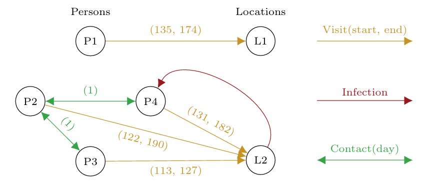
A key difference in Vahana.jl compared to most other frameworks is how agents interact with the system’s structure. In Vahana.jl, agents construct a small part of the graph \(G_{t+1}\) instead of modifying the current state of the system, e.g. by updating a variable of their own state. This simplifies parallelization and also excludes artifacts that might arise from the order in which agents carry out their transitions (Wolf et al. 2012). However, it requires that the modeller explicitly defines mechanisms to handle situations where multiple agents change the same state (e.g. compete for a resource), instead of relying on the “first-come-first-serve” behavior common in sequential systems with random agent ordering.

It would be inefficient and cumbersome to require that invariant parts of the graph (such as stable relationship networks between agents) be included in \((V'_{v,{t+1}}, E'_{v,{t+1}}) v \notin V_t\). Therefore, in Vahana.jl, when a transition function is applied, it is necessary to specify which types within the graph can potentially change. Addition ally, users can choose to retain all existing agents or edges of a given type while only adding new ones in the transition function.

The spatial layer

In Vahana.jl, (discrete) spatial information can be added via n-dimensional rasters, where the raster cells are inserted as vertices in the graph and a mapping from the Cartesian index of the underlying space to the corresponding vertices can be accessed to determine the vertex of a specific position. Since the cells are vertices of the graph, they can be treated in the same way as other agents.

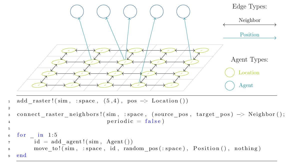
Vahana.jl provides specialized functions for creating and accessing these spatial vertices and edges between them or between agents and the spatial vertices. These edges then represent relationships such as “location \(l_1\) is a neighbor in the network of location \(l_2\)” or “agent \(a\) is located at location \(l_1\)”. Figure 2 shows an example of a graph with “spatial” vertices and edges, along with the corresponding source code that generates this structure. The key-steps involved in its construction are:

1. Raster Creation: The spatial environment in this example is initialized by creating a 5x4 raster named :space using the add_raster! function (line 1). This function requires a construction function as its final argument, which determines how each raster vertex should be initialized. Although this function receives the vertex’s position as an argument, this information is not used in this example.
2. Neighborhood Mapping: Line 3 employs connect_raster_neighbors! to establish connections (edges) between raster vertices. While this example focuses on direct neighbors, Vahana.jl supports various neighborhood definitions based on different distance metrics. With the default parameters the neighborhood structure mirrors that of a cellular automaton. Similar to the creation of vertices, the construction of edges is carried out by a function that is passed to connect_raster_neighbors!.
3. Agent Introduction & Placement: The final step (lines 6-9) introduces agents and connects them to the spatial environment. The move_to! function creates edges between agents and raster vertices. Through additional parameters (not shown here), move_to! can establish connections not only to the target vertex at position pos but also to vertices within its spatial neighborhood.



The global layer

The global layer contains vertices connected by edges to every other vertex of the graph. This is useful for providing model parameters to all or large sets of agents, collecting information from agents to generate model outputs, and aggregating information within the model to be relayed back to the agents. Figure 3 shows a graph with all three layers, where the inter-agent layer is defined as the subgraph spanned by all vertices that are neither a spatial nor a global vertex.



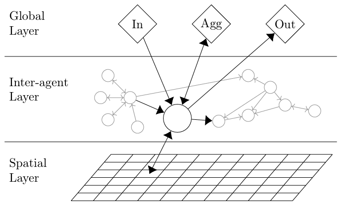
Please note that the global layer is a theoretical construct used to demonstrate that the entire simulation state can be interpreted as a single graph; for efficiency reasons, it is not actually implemented in this way. In the Vahana.jl implementation, the global layer is divided into Parameters, which remain constant throughout the simulation, and Globals. The Vahana.jl framework provides functions to compute aggregations for distributed data and to synchronously update the fields of the Globals instance.

Applicability and limitations

The ExGDS formalism is well-suited for models where agent interactions are primarily local, i.e., where agents base their decisions on the state of their direct neighbors in the graph. This covers a wide range of ABMs, including opinion dynamics, epidemiological models, and economic models with explicit network structures. Two concrete examples of such complex models — an epidemiological simulation that integrates real-world mobility data and a long-term mobility transition model with modular, plugin-based architecture — are presented in Section 7.

However, certain types of models present challenges for the ExGDS approach. Models in which agents compete for limited resources pose a particular difficulty. In sequential ABM frameworks, this is typically solved by processing the agents in random order according to the "first come, first served" principle. This approach is not possible in Vahana.jl. Instead, resources must be explicitly managed by special resource agents: Competing agents express their demand by creating edges to the resource agent, which then determines the allocation and reports the result via edges.

This can be interpreted as a parallel function call, where the edges to the resource agent represent the arguments and the edges returned by the resource agent represent the return values. While this produces additional implementation overhead, it has the advantage that it makes the interactions visible in the graph structure, which aids in debugging and understanding the model’s behavior during development.

A prominent example of such resource competition is the Schelling segregation model (Schelling 1971), where agents compete for free locations. This requires a central coordinator agent that knows all free locations and all agents wishing to move, and reassigns them accordingly. While this requires more explicit modeling effort, it has the advantage that the allocation mechanism must be explicitly specified – and can therefore be more flexibly designed – rather than being implicitly determined by a random ordering.

However, if only few resource agents exist, or a single agent must coordinate a large number of other agents, parallelization will not scale well, as a single coordinating agent corresponds to serial code - a manifestation of Amdahl’s Law (Amdahl 1967), which states that the sequential portions of a program limit the achievable speedup, regardless of how many processors are used.

A similar coordination pattern is also required when agents need to interact with other agents that are not part of their immediate neighborhood. For example, if a model provides for the random selection of agent pairs for an interaction, a coordinator agent – which has connections to all participating agents – must determine the pairings and then establish the corresponding connections between them.

In the current version, Vahana does not automatically seed random number generators or provide per-agent random streams, so reproducibility of stochastic models must be managed by the user. Explicit seeding supports repeatability for a fixed execution configuration, but identical results across different process counts are not guaranteed. To obtain process-count-invariant random draws, users can implement per-agent random streams seeded from stable logical agent identifiers that are independent of the partitioning.

Finally, models with continuous space and complex spatial neighborhood queries are currently less well supported, though we plan to address this in future work.

Implementation Example: The Hegselmann-Krause (HK) Opinion Model in Vahana.jl

To demonstrate how models are implemented in Vahana.jl, we present an implementation of the Hegselmann-Krause (HK) opinion model (Hegselmann & Krause 2002), to showcase the key concepts and typical structure of a Vahana.jl implementation.

This model describes a scenario with a finite number of agents (\(n\)). Each agent \(i\) holds an opinion denoted by \(x_i(t)\), where \(t\) represents time that moves forward in distinct steps. There is a "confidence bound" \(\epsilon>0\), meaning agents only consider the opinions of others that fall within a certain range of their own opinion. At each time step, all agents simultaneously update their opinions according to the following rule: \[x_i(t+1) = \frac{1}{| \mathcal{N}_i(t) |} \sum_{j \in \mathcal{N}_i(t)} x_j(t)\] \[\textrm{where }\quad \mathcal{N}_i(t) = \{ j \in \{1, \ldots, n\}: \| x_j(t) - x_i(t) \| \leq \epsilon \}\] In this formula, \(\mathcal{N}_i(t)\) represents the set of "neighboring" agents for agent i - those whose opinions are close enough according to the confidence bound.

The following implementation in Vahana.jl demonstrates how this model can be implemented in Vahana.jl. We will examine the implementation step by step:

using Vahana
import Statistics: mean
import Graphs: SimpleGraphs
struct Person
opinion::Float64
end
struct Knows
end
struct Params
epsilon::Float64
end

After importing the required packages, the implementation starts with the type definitions that structure our model in Vahana.jl. We define three structures:

• The Person type represents our agents.
• The Knows type is an empty structure that serves as an edge type representing which agents’ opinions are visible to others in the HK model. Since this relationship is expressed by the presence or absence of the edge itself, no additional data needs to be stored on it.
• The Params type holds our model parameters - in this case, just the confidence bound \(\epsilon\). This will be part of the global layer of our simulation.

Next, we define the model structure and create a simulation instance:

model = ModelTypes() |>
register_agenttype!(Person, :Immortal) |>
register_edgetype!(Knows) |>
create_model("Hegselmann-Krause")
sim = create_simulation(model, Params(0.2))

This two-step process reflects a fundamental concept in Vahana.jl: The distinction between a model and a simulation. The model defines the set of all possible directed graphs \(G=(V,E)\) where \(V\) consists of vertices of the registered agent types and \(E\) of edges of the registered edge types. The :Immortal hint indicates that Person agents will persist throughout the simulation, allowing Vahana.jl to optimize the underlying data access (see Section 5.2 for details on type hints).

A simulation then represents a sequence of graphs from this set, where each graph evolves into the next through transition functions. At any point in time, the simulation instance maintains only the current graph. Multiple simulations can be created from the same model definition, each potentially following different trajectories through this set of possible graphs.

The initial graph of our simulation still needs to be created:

add_graph!(sim,
SimpleGraphs.complete_graph(50),
_ -> Person(rand()),
_ -> Knows())
finish_init!(sim)

We use the add_graph! function to convert vertices and edges of a complete graph \(K_{50}\) created with Graphs.jl into agents and edges of the initial simulation graph. Two constructor functions specify how this conversion should happen: vertices are converted into Person agents with random initial opinions, while edges become Knows relationships. The call to finish_init! signals to Vahana.jl that the initial graph is completely specified - in a parallel simulation, this is where the graph is partitioned and distributed across different processes.

Finally, we define the transition function that implements the opinion update rule:

function transition(self, id, sim)
opinion_sum = self.opinion
count = 1
for other in neighborstates(sim, id, Knows, Person)
if abs(other.opinion - self.opinion) < param(sim, :epsilon)
opinion_sum += other.opinion
count += 1
end
end
Person(opinion_sum / count)
end

This function determines how each agent updates its opinion. Using neighborstates, it iterates over all agents connected via Knows edges, calculating the mean of those opinions that differ by less than \(\epsilon\) from the agent’s current opinion. The function returns a new Person instance with the updated opinion, reflecting Vahana.jl’s principle that transitions construct state rather than mutate it in place.

The transition function can now be applied to the simulation:

for _ in 1:100
apply!(sim, transition, Person, [ Person, Knows ], Person)
end

The apply! function executes the transition function for all agents of type Person. The last two arguments specify which elements of the graph are involved during this transition: [ Person, Knows ] indicates that both the state of Person agents and Knows edges might be read, while the final Person argument indicates that new states will only be produced for Person agents, while Knows edges remain unchanged. As discussed in Paragraph 3.13, this explicit specification of potential changes enables Vahana.jl to optimize the simulation by avoiding unnecessary reconstructions of unchanging graph elements.

Note that the code requires no modification to execute simulations in parallel across multiple CPU cores or even multiple nodes within a computer cluster. The sole change for a parallel run is the use of the mpirun command to initiate the simulation.

Implementation Aspects

This section explores the interplay of data distribution, performance optimization, and reliability within Vahana.jl simulations.

Type hints

In Vahana.jl, the code for accessing and managing the state of the model is generated dynamically at runtime, taking advantage of Julia’s Just-In-Time compilation. Methods in Julia are compiled for each specific type combination the first time they are called, and Vahana.jl tailors the code to be compiled according to so-called ‘hints’ provided for the edge or agent types. This code generation process enables optimization of data structures like the adjacency matrix and their access functions, ensuring efficient state access and management.

Edge hints are optional traits that can be assigned to edge types. These hints provide Vahana.jl with insights into how edges of a specific type are utilized within transition functions. Table 1 describes some edge hints and their effects.

Table 1: Edge type hints.

Hint	Contract or Effect
IgnoreFrom	Vahana.jl omits storing the source vertex ID.
IgnoreSourceState	The state of the agent at the source of the edges are not accessed.
SingleEdge	Each target vertex has at most one edge of this type.
SingleType	All target vertices are guaranteed to be of the same type.
Stateless	Only the source vertex ID is stored.

To illustrate the influence of type hints on the generated code, Figure 4 shows two variants of the add_edge! function. Although simplified for clarity, they represent the essence of the code after inlining and compiler transformations and show how variations in hints can lead to drastically different code.



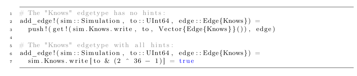
The first implementation handles edge types without any optimization hints, relying on operations such as dictionary lookups or array appends. On an AMD Ryzen 9 7900X CPU, a call to this version requires an average of 18.6 ns (nanoseconds). In contrast, the second implementation, optimized with all hints activated, reduces the average execution time by more than 75%, to just 4.5 ns.

For agents, there exists only one hint, informing Vahana.jl that agents of a given type are Immortal. To utilize the MPI-3 shared memory, Vahana.jl stores agents in a contiguous block of memory. This requires tracking the “alive” state of mortal agents. When the Immortal hint is applied to an agent type, it means that this agent type will persist throughout the simulation, and therefore it is not necessary to track the “alive” state.

These hints can be seen as contracts that define the expected behavior and interactions between agents, edges, and other components of a model. Violating this contract can lead to unpredictable and erroneous simulation results. To safeguard against such contract violations, Vahana.jl by default performs checks that identify and flag potential contract breaches. However, once a model has been thoroughly tested and verified, these checks can be disabled for performance optimization.

Data distribution

In parallelized simulations, the distribution of data across multiple processes is crucial for dealing with computationally intensive problems. Vahana.jl shields users from the complexities of low-level distributed programming. Under the hood, Vahana.jl leverages the Message Passing Interface (MPI), a standardized and widely adopted communication protocol for distributed computing.

In distributed Vahana.jl simulations, a fundamental design principle is that each computational process knows only a subset of the graph representing the current simulation state. Edges are always stored in the process that manages the vertex at the edge’s target, as this agent must know of the edge’s existence and can access its state during transition functions.

Vahana.jl offers three mechanisms for distributing agents across processes. By default METIS (Karypis & Kumar 1998) is used for graph partitioning. For models with different agent types, a round-robin scheme per agent type is available as an alternative, which ensures that each agent type is evenly distributed across processes - a constraint that METIS cannot guarantee, since it does not distinguish between agent types. Finally, modellers can provide custom partitioning information, as was done in the MATSim-Episim reimplementation.

New agents created during a simulation are assigned to the process of the agent whose transition function called add_agent!. Currently, Vahana.jl does not support dynamic load balancing, which can lead to imbalances in simulations with highly dynamic graph structures.

Since an agent \(v\) can access its 1-neighborhood subset (\(G'_{v,t}\)), the process that manages \(v\) must also have knowledge of the states of the agents that are located at the source of the incoming edges to \(v\). To optimize performance, Vahana.jl uses MPI-3 shared memory to avoid redundant copies of agents residing on the same compute node as the agent \(v\). Only when agents in \(G'_{v,t}\) are managed by a different node is their state transferred to the process which handles agent \(v\).

Vahana.jl uses a double buffering approach for state management: Read buffers contain the current vertices and edges for all types in the ‘read’ argument of the apply! function, while write buffers collect the new vertices and edges that are generated during transitions for all types in the ‘write’ argument. Figure 5 illustrates this mechanism using the epidemiological model from Figure 1 during the execution of a transition where locations determine whether a person has been infected. The figure shows the intermediate state within the apply! function: read buffers are marked in green and write buffers in red. The graph is distributed across two compute nodes, each with two processes. Solid borders indicate data that originates from and remains on the local process, while dashed borders represent data involving other processes.



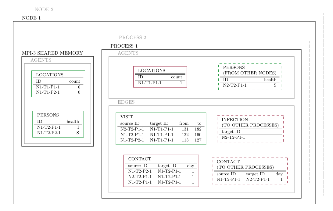
In this model, the state of the Person agents consists of their health status (S for susceptible, I for infected, R for recovered), while the state of the Location agents is a counter representing the number of people who have been infected at that location.

For illustration purposes, we depict the IDs in the format N(ode)-T(ype)-P(rocess)-index, where the index distinguishes multiple agents of the same type within the same node and process. T1 represents Location agents and T2 represents Person agents. The agents from Figure 1 correspond to the illustration IDs shown in Table 2.

Table 2: Mapping of agent identifiers in different figures.

Figure 1	Figure 5
P1	N2-T2-P2-1
P2	N1-T2-P1-1
P3	N1-T2-P2-1
P4	N2-T2-P1-1
L1	N1-T1-P2-1
L2	N1-T1-P1-1

Synchronization across processes works as follows: Before executing any transition functions, Vahana.jl checks for each readable agent type whether the agent states may have changed since the last synchronization and whether any edge type in the read argument provides access to the state of the agents on the source side of the edges. When synchronization is needed, Vahana.jl transmits agent states to processes where these agents appear as sources of edges, creating local copies (ghost agents). In our epidemiological example, since person health states may have changed since the last transition and location agents need to access the health status of visiting persons, synchronization of person states across processes is necessary.

To complete the apply! function, Vahana.jl distributes the newly created edges targeting agents in remote processes using MPI’s all-to-all communication patterns. For edges, the write buffers then become the new read buffers for the next transition phase, while for agents, the states from different processes on a single node are consolidated into a single MPI-3 shared memory block.

Performance Analysis

In this section, we evaluate Vahana.jl’s performance characteristics using the Hegselmann-Krause (HK) opinion model as a standardized benchmark. The HK model was chosen because its agents perform relatively simple calculations that depend primarily on the state of other agents, making framework overhead particularly apparent. Beyond comparing against custom-tailored implementations, we also evaluate how Vahana.jl performs relative to other established frameworks, both single-threaded (NetLogo, Agents.jl) and HPC-enabled (FLAME, Repast4Py, FPMAS).

The single-threaded benchmarks were performed on a desktop computer equipped with an AMD Ryzen 9 7900X CPU and 32 GB of RAM. The parallel benchmarks and additional framework comparisons were conducted on the Emmy cluster at NHR@Göttingen and the Lise cluster at Zuse Institute Berlin, both featuring nodes with two Intel Cascade Lake Platinum 9242 processors (48 cores each) and 384 GB of memory.

The Hegselmann-Krause (HK) opinion model

When evaluating ABM frameworks, an important question is how much performance overhead they introduce compared to custom-tailored implementations. This overhead becomes particularly apparent in models where agents perform relatively simple calculations that depend primarily on the state of other agents and do not require complex internal calculations. The HK model previously used as an implementation example is therefore an ideal test case for such a performance analysis.

Beyond comparing against custom-tailored implementations, we also evaluate how Vahana.jl performs relative to other established frameworks. We begin this comparison with non-HPC frameworks that execute simulations on a single thread: NetLogo (v7.0.3) (Wilensky 1999), one of the most widely adopted ABM platforms in the social sciences, and Agents.jl (v6.2.10) (Datseris et al. 2024), which is a relatively new Julia-based framework whose developers emphasize performance as an important design goal and which achieves strong results in their own benchmarks compared to other frameworks. To evaluate the parallel capabilities of Vahana.jl, we will later present comparisons with HPC-enabled frameworks: FLAME (v0.3.1), Repast4Py (v1.1.4), and FPMAS (v1.6).¹

All performance measurements focus solely on the computation time of the opinion updates, excluding both the initial setup costs such as graph generation and partitioning, and, in case of the Julia implementations, the Just-In-Time compilation time.

Single-threaded performance comparison

Figure 6 shows how long a single iteration takes for a HK simulation with 100 and 10,000 agents on a complete graph. Two variants of Vahana.jl (v1.4.7) are shown: “Vahana.jl” uses no hints, while “+ hints” applies the :Immortal hint to the Person agent type and the :SingleType and :Stateless hints to the Knows edge type, enabling the optimized data access described in Section 5. The “Direct” implementation is a custom Julia implementation that operates directly on arrays of agent opinions. All implementations ensure synchronous opinion updates: The direct implementation uses double buffering, NetLogo and Agents.jl manage the state of agents with fields old_opinion and new_opinion, and have a “new to old” copy step after all agents have calculated their new_opinion, while Vahana.jl provides this synchronous behavior natively through its framework design.



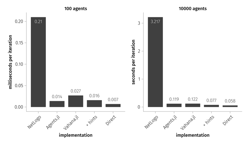
The computational workload increases by a factor of approximately 10,000 when scaling from 100 to 10,000 agents, as we have a hundred times more agents, each of which compares its opinion with a hundred times more neighbors (the exact factor varies slightly due to confidence bound filtering). For an implementation that requires 1 ms per iteration with 100 agents, perfect linear scaling would mean 10 seconds per iteration for 10,000 agents.

Results that are higher than this scaling expectation, as observed in NetLogo (3.217 seconds versus an expected 2.1 seconds), suggest that this framework exhibits performance characteristics that do not scale perfectly with problem size. The analysis of the exact reason (whether due to memory allocation patterns, inefficiencies in the data structure, or other framework-specific implementation details) would require detailed profiling and is beyond the scope of this article. Conversely, implementations that achieve better than expected performance, such as the Direct implementation, Agents.jl, and Vahana.jl, benefit from the fact that the fixed overhead becomes relatively less significant as computational intensity increases. Notably, with hints applied, Vahana.jl (0.077 s) approaches the performance of the Direct implementation (0.058 s) at 10,000 agents, demonstrating that the type hints effectively reduce the framework overhead.

In the first comparison, all implementations simulate scenarios in which each agent takes into account the opinions of all other agents. Although this corresponds to the original HK model formulation, it is unrealistic for real social networks. All previous implementations (apart from Vahana.jl, which by its design always generates a graph) have taken advantage of this and bypassed any functionality required for a potential graph structure. However, this also means that in these implementations, the complete graph cannot be be easily replaced by other graph structures without significant code changes. To enable a more realistic comparison that better reflects typical ABM requirements, and to investigate the impact of Vahana.jl’s inherent graph structure on performance, we have additionally implemented versions for NetLogo and Agents.jl that generate explicit networks between agents, and added a Julia implementation using the Graphs.jl package to replace the minimal "Direct" implementation. Figure 7 shows the results of these network-based implementations.



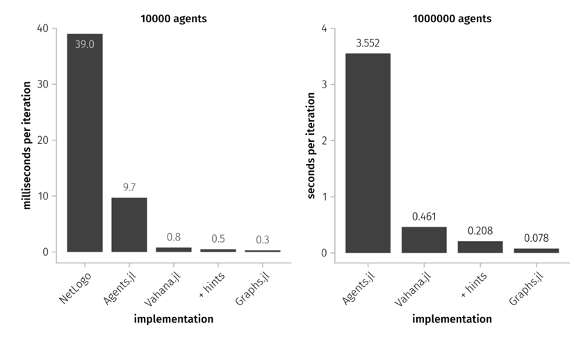
The network-based implementations exhibit different performance characteristics compared to the full graph scenario. With 10,000 agents, Vahana.jl with hints (0.5 ms) is 19 times faster than Agents.jl with Graphs.jl integrated (9.7 ms) and 78 times faster than NetLogo (39 ms), though it is slower than the Graphs.jl only implementation (0.3 ms). Notably, while Agents.jl performed competitively in the complete graph scenario, the integration of an explicit graph structure via Graphs.jl introduces substantial overhead, making it significantly slower than Vahana.jl.²

When scaling from 10,000 to 1,000,000 agents, most implementations show sublinear scaling due to memory access bottlenecks at larger problem sizes. The Graphs.jl implementation demonstrates the most efficient scaling, increasing execution time by a factor of 260 compared to the theoretical 100-fold increase expected for perfect linear scaling. Vahana.jl shows less favorable scaling characteristics, with performance degrading by factors of 416 (with hints) and 576 (without hints). NetLogo’s scalability issues are most severe, failing to complete the one million agent simulation within an hour, highlighting the performance limitations of this widely-used platform for large-scale simulations.

At this scale, Graphs.jl outperforms Vahana.jl by approximately 3 times (78ms vs 208ms). However, this single-threaded advantage disappears when parallelization is considered: while the Graphs.jl implementation cannot be easily parallelized, Vahana.jl achieves better performance than single-threaded Graphs.jl when using 4 or more processes.

Comparison with HPC-enabled ABM frameworks

The frameworks discussed so far cannot distribute the calculation of a single simulation across multiple CPU cores or cluster nodes. To fully evaluate Vahana.jl’s capabilities, we now compare it with frameworks that support high-performance computing environments: FLAME, Repast4Py, and FPMAS, which were introduced in the Related Work section.

We conducted benchmarks using graphs where each agent has exactly 50 neighbors, rather than being fully connected. The test scenario comprised 39,936 agents with a confidence bound of 0.2. This relatively modest size was chosen due to technical limitations: the graph generation algorithm in our Repast4Py implementation exhibited unexpected quadratic time complexity, while FPMAS encountered segmentation faults during partitioning for graphs exceeding 300,000 agents. Moreover, the Repast4Py implementation required the number of agents to be evenly divisible by the number of processes.

However, our evaluation of FLAME revealed several significant limitations that prevent a meaningful comparison with the other HPC-enabled frameworks. Even for complete graph structures, FLAME performs substantially worse than Vahana.jl, being 16.5 times slower in the best case (utilizing 96 threads). For sparse network structures like our 50-neighbor graphs, FLAME’s message board architecture requires either broadcasting all messages to all agents, making it approximately 1000 times slower than Vahana.jl, or pre-defining filters in XML files with, in our use case, 14 million lines.

Additionally, we were unable to deploy FLAME across multiple cluster nodes, and its dependency on the outdated OpenMPI version 3 makes installation particularly cumbersome on modern HPC systems. Given these technical limitations, along with FLAME’s apparent discontinuation in favor of FLAME GPU (which targets GPU architectures that are outside the scope of this comparison), we excluded FLAME from the following analysis.

Figure 8 shows significant performance differences between the frameworks. Vahana.jl requires 75ms per iteration with a single process, compared to 583ms for Repast4Py and 243ms for FPMAS. FPMAS’s performance degrades when scaling to multiple processes. This might be related to its approach of synchronizing agent states in distributed environments. FPMAS supports two methods for converting agent data for transfer between processes (called serialization) — one using a human-readable text format (JSON) and another using a more efficient binary format. In our benchmarks we use the binary method, which still shows limited scalability in our tests, reaching a maximum speedup of only 1.5 at 384 processes.



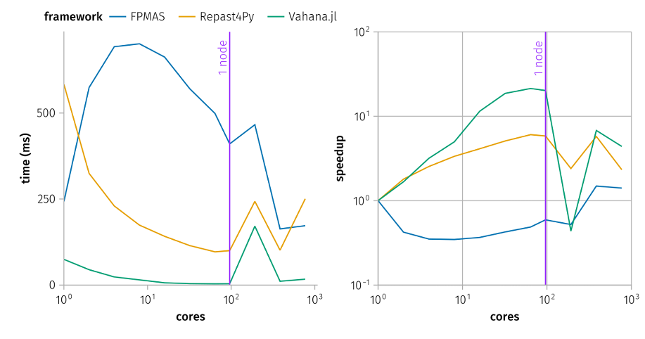
Repast4Py shows steady performance improvements up to 64 processes, achieving a speedup of about 6. Like FPMAS, it implements manual serialization for state synchronization. The relative stability of its performance might be due to the computational costs of the opinion updates dominating the synchronization overhead, though this would need to be confirmed through profiling.

Vahana.jl takes a different approach by leveraging MPI shared memory within a node, allowing direct access to agent states without serialization, reaching a speedup of 20 with 96 processes (a single node). When scaling beyond a single node, it uses MPI derived datatypes for state transfer. While this avoids explicit serialization, the additional overhead for transferring agent states between nodes still impacts performance. This explains the general performance decrease with multiple nodes, but not the significant spike to 171ms per iteration at 192 processes (2 nodes), which appears to be an anomaly given the better performance with 4 and 8 nodes.

Case Studies

While Section 6 evaluated Vahana.jl’s performance characteristics through a standardized benchmark, this section demonstrates its ability to express complex, real-world models. We present two implementations that differ substantially in their domain, structure, and the Vahana.jl features they exercise: a reimplementation of the MATSim-Episim epidemiological model, and MoTMo, a long-term mobility transition model.

MATSim-Episim: Integrating mobility data with disease dynamics

MATSim-Episim is a large-scale agent-based epidemiological model that combines a person-centric mobility model with a mechanistic model of infection and disease progression (Müller et al. 2021). It builds on the multi-agent transport simulation MATSim (Horni et al. 2016) and was regularly used during the COVID-19 pandemic to advise the German federal government (e.g., Müller et al. 2021). A simplified version of this model was introduced in Figure 1 to illustrate the ExGDS formalism. The full reimplementation³ demonstrates how Vahana.jl can express a model in which different agent types have fundamentally distinct roles within a coordinated daily cycle.

Five agent types structure the simulation: Person agents carry a health state and an age that influences disease progression; Facility and Vehicle agents represent locations where contacts occur and actively mediate disease transmission by processing the simultaneous presence of persons; HealthAuthority performs contact tracing; and a single World agent introduces new infections from outside the population. Eleven edge types with carefully applied type hints capture the full range of interactions: daily activity schedules are modeled through MaybeEvent and ActiveEvent edges, disease transmission through Infect and DiseaseImport edges, and public health interventions through Contact, InformInfection, and HealthStateChange_ edges.

A single simulated day is decomposed into seven transitions, each applied to the relevant agent types. The day begins with disease import, where the World agent selects random persons for exposure. Activity participation is then filtered according to policy-driven restrictions and individual quarantine status. At each Facility and Vehicle, the contact model samples co-present persons and computes transmission probabilities based on contact intensity, duration, mask usage, and age-dependent susceptibility — with new Infect edges created where transmission occurs. Subsequent transitions handle infection checking, disease progression through an eight-state health model, and contact tracing via the HealthAuthority, which samples reported cases up to a capacity limit and recursively notifies contacts. Each day concludes with aggregated health reporting using Vahana.jl’s distributed map-reduce functionality.

The implementation also demonstrates Vahana.jl’s support for domain-specific partitioning. Rather than relying on generic graph partitioning, the model uses a custom heuristic that assigns locations to processes based on their event load and co-locates persons on the same node as the majority of their visited locations — exploiting the model’s known structure to minimize cross-process communication during the contact model transitions. The model was tested at two scales: a Berlin scenario with 1.0 million agents, 0.9 million locations, and 6.8 million daily location visits, and a Germany-wide scenario with 16.3 million agents, 11.5 million locations, and 91.5 million daily visits.

Figure 9 shows the scalability results for both scenarios. The plot on the left presents the overall runtime for simulating one year, while the figure on the right illustrates the speed-up achieved. The Berlin scenario is not large enough to benefit from distribution across multiple nodes on the Lise compute cluster. For the Germany scenario, we achieve a reduction to 22.5 minutes with 8 nodes, which is 207 times faster than the 3.2 days needed to calculate the Germany scenario with a single thread.



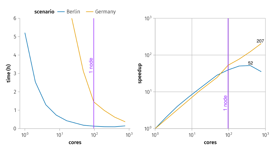
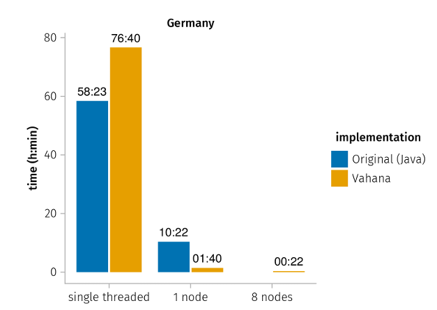
Figure 10 presents a performance comparison between our Vahana.jl implementation and the original Java-based MATSim-Episim for the Germany scenario. This comparison should be viewed with some caution, as it was not checked whether the version from the MATSim-Episim repository⁴ includes additional features not described in Müller et al. (2020). Note that MATSim-Episim utilizes Java Parallel Streams for its most computationally intensive loops, restricting parallelization to a single node (Fürst & Rakow 2022). Despite the slower single-thread performance of Vahana.jl compared to the Java version, it shows remarkable advantages when parallelized: when using a single node, Vahana.jl outperforms the original MATSim-Episim implementation by a factor of 7, and when scaled to 8 nodes, this advantage increases to a factor of 28.



MoTMo: A Modular Mobility Transition Model

The Mobility Transition Model (MoTMo)⁵ is a large-scale agent-based model built on Vahana.jl for analyzing long-term mobility transitions. Developed as part of the Digital Triplet for Sustainable Mobility (DiTriMo) project⁶, it simulates car ownership decisions across decades, driven by life course events such as aging, household formation, job changes, and income shifts. MoTMo is designed as a modular model architecture: rather than encoding a single fixed theory, it decomposes behavior into interchangeable modules that can be recombined to explore alternative assumptions. The DiTriMo implementation described here represents the first concrete application of this architecture.

The model comprises four agent types – Person, Household, WorkPlace, and Cell – and seven edge types representing household membership, spatial location, employment, and mobility tool negotiations. Persons hold attributes for demographics, income, and mobility availability; households aggregate person-level demand and approve or deny mobility requests; workplaces extend persons with job-related spatial context; and cells serve as spatial units for regional aggregation.

MoTMo achieves its modular structure through a system of ten ordered substeps that structure each timestep. Behavioral modules attach their transition functions to specific substeps, optionally with a priority level that determines the execution order when multiple modules attach transitions to the same substep. For example, the check_for_changes substep is responsible for handling life-course events such as aging or household formation, while reconsider_mob_avail evaluates car ownership decisions, and update_usage aggregates mobility statistics. Each module exists in multiple variants: the demographic module alone comprises five implementations that can be selectively combined, spanning from simple aging to detailed household formation and breakup. Simulation configurations select which variant of each module to activate, enabling researchers to compose distinct model versions from a shared component library and to compare, for example, rational-actor against bounded-rationality assumptions within an otherwise identical structural setup.

The DiTriMo implementation has been applied to the Lausitz region in eastern Germany and to Berlin. The Lausitz scenario comprises approximately 250,000 person agents and 120,000 households, where each agent represents four individuals; the Berlin scenario is roughly twice as large, with each agent representing ten individuals. Simulations run from 2020 to 2035 in quarterly time steps, tracking the evolution of car ownership and spatial mobility distributions under varying policy assumptions. While the architecture could in principle support one-to-one population scales, the current aggregation level reflects both the availability of MATSim input data (synthetic populations and activity schedules generated by MATSim) and the limited marginal gain of finer resolution at the present stage of model development.

We have not conducted a systematic performance study for MoTMo, as runtimes depend strongly on the chosen module configuration. However, to provide a rough sense of computational cost: for the Berlin scenarios in the DiTriMo project, running on the AMD Ryzen 9 7900X desktop processor described in Section 6 and parallelized across 8 cores, a single simulation step requires approximately 2 seconds. The complete simulation, including reading all required input files and initial code compilation, takes roughly 5 minutes for the first run and approximately 3 minutes for subsequent runs.

Conclusion

In this paper, we introduced Vahana.jl, an ABM framework that supports simulations at various scales, from single computers to large-scale HPC environments, while simplifying the development of parallel simulations.

We have outlined the theoretical foundations and design principles of Vahana.jl. Its unique approach of representing the entire simulation state as a graph allows researchers to naturally model and analyze systems with intricate network structures and interactions. This approach has been proven capable of facilitating the development of complex ABMs, as demonstrated through the MATSim-Episim reimplementation and the MoTMo mobility transition model.

Our performance analysis demonstrates that Vahana.jl is a compelling choice for researchers, particularly when network interactions between agents are crucial. Notably, it enables researchers to tackle significantly larger and more complex problems, thereby enhancing the scope and potential of their simulations.

Vahana.jl is not limited to large-scale simulations; it is also a powerful tool for researchers studying the dynamics of networks, regardless of scale. Its design philosophy prioritizes network interactions and relationships, making it a valuable tool for various research applications.

While Vahana.jl currently prioritizes network interactions, we plan to extend its support for spatial elements by introducing continuous-space coordinates and efficient spatial neighborhood search. In the current implementation, as demonstrated in the Vahana.jl tutorials⁷, identifying agents within a spatial neighborhood is an unnecessarily complex process. Improving this functionality will simplify spatial queries and enhance usability.

Future work will also focus on further performance improvements, particularly through the implementation of dynamic load balancing and more sophisticated partitioning strategies for heterogeneous agent types and spatial structures. These challenges are the focus of the project "Advanced Partitioning Methods for High-Performance Agent-Based Simulations", funded by MATH+.

References

Abar, S., Theodoropoulos, G. K., Lemarinier, P., & O’Hare, G. M. P. (2017). Agent based modelling and simulation tools: A review of the state-of-art software. Computer Science Review, 24, 13–33. [doi:10.1016/j.cosrev.2017.03.001]

Adiga, A., Kuhlman, C. J., Marathe, M. V., Mortveit, H. S., Ravi, S. S., & Vullikanti, A. (2018). Graphical dynamical systems and their applications to bio-social systems. International Journal of Advances in Engineering Sciences and Applied Mathematics, 11(2), 153–171. [doi:10.1007/s12572-018-0237-6]

Amdahl, G. M. (1967). Validity of the single processor approach to achieving large scale computing capabilities. Proceedings of the April 18–20, 1967, Spring Joint Computer Conference. [doi:10.1145/1465482.1465560]

Bezanson, J., Karpinski, S., Shah, V. B., & Edelman, A. (2012). Julia: A fast dynamic language for technical computing. arXiv preprint. Available at: https://arxiv.org/abs/1209.5145.

Breugnot, P., Herrmann, B., Lang, C., & Philippe, L. (2021). A synchronized and dynamic distributed graph structure to allow the native distribution of multi-agent system simulations. 2021 29th Euromicro International Conference on Parallel, Distributed and Network-Based Processing (PDP). [doi:10.1109/pdp52278.2021.00017]

Coakley, S., Richmond, P., Gheorghe, M., Chin, S., Worth, D., Holcombe, M., & Greenough, C. (2016). Large-scale simulations with FLAME. In J. Kołodziej, L. Correia, & J. M. Molina (Eds.), Intelligent Agents in Data-intensive Computing (pp. 123–142). Cham: Springer International Publishing. [doi:10.1007/978-3-319-23742-8_6]

Collier, N., & Ozik, J. (2022). Distributed agent-based simulation with Repast4Py. 2022 Winter Simulation Conference (WSC). [doi:10.1109/wsc57314.2022.10015389]

Crooks, A., Heppenstall, A., & Malleson, N. (2018). Agent-based modeling. In B. Huang (Ed.), Comprehensive Geographic Information Systems (pp. 218–243). Amsterdam: Elsevier. [doi:10.1016/b978-0-12-409548-9.09704-9]

Datseris, G., Vahdati, A. R., & DuBois, T. C. (2024). Agents.jl: A performant and feature-full agent-based modeling software of minimal code complexity. SIMULATION, 100(10), 003754972110688. [doi:10.1177/00375497211068820]

Fürst, S., & Rakow, C. (2022). Parallelization of large-scale agent-based epidemiological simulations. Proceedings of the 34th European Modeling Simulation Symposium (EMSS 2022).

Gutowitz, H. (1991). Cellular Automata: Theory and Experiment. Cambridge, MA: MIT Press.

Hegselmann, R., & Krause, U. (2002). Opinion dynamics and bounded confidence models, analysis and simulation. Journal of Artificial Societies and Social Simulation, 5(3), 2.

Horni, A., Nagel, K., & Axhausen, K. W. (2016). The Multi-Agent Transport Simulation MATSim. London: Ubiquity Press.

Karypis, G., & Kumar, V. (1998). A fast and high quality multilevel scheme for partitioning irregular graphs. SIAM Journal on Scientific Computing, 20(1), 359–392. [doi:10.1137/s1064827595287997]

Kravari, K., & Bassiliades, N. (2015). A survey of agent platforms. Journal of Artificial Societies and Social Simulation, 18(1), 11. [doi:10.18564/jasss.2661]

Kuhlman, C. J., Anil Kumar, V. S., Marathe, M. V., Mortveit, H. S., Swarup, S., Tuli, G., Ravi, S. S., & Rosenkrantz, D. J. (2011). A general-purpose graph dynamical system modeling framework. Proceedings of the 2011 Winter Simulation Conference (WSC). [doi:10.1109/wsc.2011.6147758]

Müller, S. A., Balmer, M., Charlton, W., Ewert, R., Neumann, A., Rakow, C., Schlenther, T., & Nagel, K. (2020). A realistic agent-based simulation model for COVID-19 based on a traffic simulation and mobile phone data. arXiv preprint. Available at: https://arxiv.org/abs/2011.11453. [doi:10.1101/2021.02.27.21252583]

Müller, Sebastian A., Balmer, M., Charlton, W., Ewert, R., Neumann, A., Rakow, C., Schlenther, T., & Nagel, K. (2021). Predicting the effects of COVID-19 related interventions in urban settings by combining activity-based modelling, agent-based simulation, and mobile phone data. PLoS One, 16(10), e0259037. [doi:10.1371/journal.pone.0259037]

Müller, Sebastian Alexander, Charlton, W., Conrad, N. D., Ewert, R., Jefferies, D., Rakow, C., Wulkow, H., Conrad, T., Schütte, C., & Nagel, K. (2021). MODUS-COVID bericht vom 09.04.2021. Technical report, Technische Universität Berlin. http://dx.doi.org/10.14279/depositonce-11772

Polhill, G., Heppenstall, A., Batty, M., Salt, D., Colasanti, R., Milton, R., & Hare, M. (2023). Exascale computing and “next generation” agent-based modelling. Review of Artificial Societies and Social Simulation. Available at: https://rofasss.org/2023/09/29/exascale-computing-and-next-gen-abm/. [doi:10.65109/vdxj1108]

Railsback, S. F., & Grimm, V. (2011). Agent-Based and Individual-Based Modeling: A Practical Introduction. Princeton, NJ: Princeton University Press.

Richmond, P., Chisholm, R., Heywood, P., Chimeh, M. K., & Leach, M. (2023). FLAME GPU 2: A framework for flexible and performant agent based simulation on GPUs. Software: Practice and Experience, 53(8), 1659–1680. [doi:10.1002/spe.3207]

Rousset, A., Herrmann, B., Lang, C., & Philippe, L. (2016). A survey on parallel and distributed multi-agent systems for high performance computing simulations. Computer Science Review, 22, 27–46. [doi:10.1016/j.cosrev.2016.08.001]

Schelling, T. C. (1971). Dynamic models of segregation. Journal of Mathematical Sociology, 1(2), 143–186.

Tesfatsion, L., & Judd, K. L. (2006). Handbook of Computational Economics, Volume 2: Agent-Based Computational Economics (Handbook of Computational Economics). Amsterdam: North-Holland Publishing Co.

Wilensky, U. (1999). NetLogo. Center for Connected Learning and Computer-Based Modeling, Northwestern University, Evanston, IL.

Wolf, S., Fürst, S., Mandel, A., Knell, S., Lass, W., Lincke, D., Teitge, J., & Jaeger, C. (2012). Two modes of scheduling in a simple economic agent-based model. SIMULTECH 2012 – Proceedings of the 2nd International Conference on Simulation and Modeling Methodologies, Technologies and Applications, Rome, Italy, 28 - 31 July, 2012. 2012.