Hu Bin and Debing Zhang (2006)

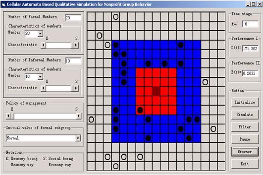
Cellular-Automata Based Qualitative Simulation for Nonprofit Group Behavior

Journal of Artificial Societies and Social Simulation vol. 10, no. 1
<https://www.jasss.org/10/1/1.html>

For information about citing this article, click here

Received: 27-Dec-2005    Accepted: 07-Dec-2006    Published: 31-Jan-2006

Abstract

A cellular automata based qualitative simulation of group behavior (referred hitherto as 'loyalty to group') will be presented by integrating QSIM (Qualitative SIMulation) and CA (Cellular Automata) modeling. First, we provide a breakdown of the structure of a group and offer an analysis of how this structure impacts behavior. The characteristics and impact had by anomalies within a group and by environmental factors are also explored. Second, we explore the transition between cause and effect (referred hitherto as the 'transition rule') and the change in behavior that is the result of this transition (referred hitherto as the 'successor behavior state'). A filter for weeding out anomalies is then proposed. The simulation engine is then used integrating all relevant data as outlined above. A concept referred to as the 'Loyalty-cost equilibrium' is presented and factored into the filter. Third, the validity of this method is tested by running the simulation using eight generalized examples. The input-output of each simulation run using these examples is consistent with what can reasonably be accepted to be true, thus demonstrating that the proposed method is valid. At this point we illustrate how the simulation is applied in context. Simulation outputs (effect on group behavior) at each time stage of two alternating changes in policy are compared to determine which policy would be the most advantageous. This demonstrates that this method serves as reliable virtual tool in the decision making difficulties of group management.

Keywords:

Cellular Automata; Qualitative Simulation; Group Behavior; Loyalty-Cost Equilibrium; Loyalty Gravitation; Cost Gravitation

Introduction

1.1

Computer simulation has long been a tool used in the natural sciences. In management science however, with the exception of those systems employed at an operational level (e.g. production and inventory) computer simulation has been considered inappropriate (Berends and Romme 1999). Traditional computer simulation generates output mathematically, and the data related to difficulties faced when dealing with people (e.g. Human resources management and Marketing) is too complex, ambiguous, and imprecise to be assessed mathematically.

1.2

Here we propose a qualitative simulation method of predicting how and to what effect a group is likely to evolve. This is the foundation to achieve qualitative simulation for explaining complexity in management science, since the complexity is primarily emerged from individual or group behavior.

1.3

Qualitative simulation was originally proposed to explore the behavior of physical systems. In this field QSIM algorithm has been accepted widely (Kuipers 1986). It models the simulated object by qualitative differential equations. The simulation process is as follows:

• Generate all possible successor states of variables.
• Filter abnormal successor states using constraints.
• Form combinations among remaining successor states.
• Filter abnormal combinations using a global filter.

1.4

In our opinion, the key component of QSIM is the filter. It is with the filter that we have endeavored to adapt the QSIM for the CA modeling of group behavior.

1.5

For a management system (any organizational structure concerned with the management of people), QSIM has been inappropriate due to the complexity and ambiguity inherent when dealing with people. Factors to be considered include:

• Behavioral Unpredictability: The principle concern of any management system is people, customers as well as employees, and people often behave in unexpected ways. Motivations and behaviors can and do change abruptly and without warning. An equation-based method of analysis like the QSIM is therefore unsuited to the challenges faced by a management system.
• Impact of Internal and External Environment: Management systems are affected by the environment within which they operate. External political, economic, societal/cultural and technological factors all can influence change in behavior, as well as internal environmental factors, such as managerial policy (i.e. incentives offered by management) and organizational culture. The environment is also apt to change in unexpected ways since its changes are largely dictated by changes amongst individuals operating within it. Naïve systems (the tube system or the spring/mass system) are not designed for this degree of uncertainty.

1.6

In the social sciences the DST (Dynamical systems theory) has served as a tool for analysis in various areas of psychology such as perception, attention, speech production and human development. Vallacher and Nowak (1994), using the DST, were able to encompass the dynamic and complex nature of social psychological phenomena. They have also written on the validity of dynamical systems as applied to, along with various concepts and methods (including CA) associated with, social psychological study (Vallacher and Nowak 1997). From Vallacher and Nowak's work, we learn that the heart of social psychology is found amongst complex causalities. Agent based simulation has been employed to demonstrate the dynamics of reputation and social order in artificial societies. Amongst the areas studied were the connection between image and reputation, as well as the factors by which each is influenced (Conte and Paolucci 2002). Reputation is seen as an agent property resulting from the agents' socially desirable behavior such as cooperation, altruism, reciprocity, conformity or subservience. An agent is combined with data resulting from the complex interplay of the above within a simulation, resulting in a yield of useable data. This research highlights the importance of qualitative simulation in the study of group behavior. Using CA allows one to navigate effectively the complexities of group dynamics by following the rules of interaction among members. Each agent is represented by a cell.

1.7

CA was originally intended exclusively for use in study of the natural sciences. It was within the last decade that CA have been used frequently in the behavioral and social sciences, including changes in attitude, pricing in a spatial setting, the dynamics of cooperation and socialization, etc. (Hegselmann and Flache 1998).

1.8

CA can be seen as a type of socio-matrix. In Klüver and Stoica (2003), CA is used to predict changes within a group. It comes to two conclusions: 1) behavior of group members can be determined by values within the matrix; and 2) the process of making friends can be simulated.

1.9

Our research on CA methods as applied to the social sciences can be summarized as thus:

• "Group behavior" refers to an action taken by an individual or individuals relating to and/or impacting the group, such as making friends or choosing a seat according to who else is sitting near it, thus selecting with whom they will be interacting on a regular basis. In the real world however, there is much more that must be taken into consideration. Behavior varies widely and often unpredictably, a result of "norms" that differ according to context. How individuals within management circles co-operate with each other, and how loyal they are to the group, will differ from the same amongst employees.
• The methodology is not perfect. Cells (representing members of a group) and the result of their interaction within the group are represented on a lattice. This representation is strictly visual and can be misleading. Take for example the question of whether or not group members with analogous behavior locate together on the lattice. If they do, then the group is formed. If they do not, then the group is not formed. In the real world however, group members locating together might indicate nothing beyond the fact. While commonalities do exist from interaction to interaction, they are not absolutes and thus CA modeling can not be considered foolproof.

1.10

Using CA modeling, we explore how group behavior evolves from the perspective of qualitative simulation. For the purposes of this paper, the loyalty of individuals to the group is simulated. How loyally individuals are likely to behave will depend on the character of each individual considered in combination with the effect had by managerial policy (i.e. incentives). Other factors must also be considered. This example relates generally to a spectrum of behaviors that can be simulated using qualitative simulation and is therefore representative and valid overall.

1.11

The issue of group loyalty can be viewed as a system issue: A group is a system involving input and output.

1.12

Input is how loyal group members are initially, or the "loyalty state" of the group, when management offers a new policy (i.e. incentive). The initial loyalty state is represented by cells and is determined according to the characteristics of individual members. The new policy is the factor expected to affect a transition from one loyalty state to another.

1.13

"Transition rules" are designed to represent how members interact with each other (according to specific characteristics) as well as how they respond to managerial policy (i.e. incentives). Outputs are generated by applying these rules.

1.14

Output is comprised of the loyalty state and a corresponding evaluation. Loyalty states are represented graphically in cell formations on a lattice. Because the interaction between individuals may result in many combinations of cell formations at each time step, the purpose of evaluation is to determine which cell formation is most probable, or in other words, which loyalty state will most likely be affected by the new policy. It is at this point a filter is integrated (and, for the purposes of this paper, discussed).

1.15

The method of filtering proposed by this paper is the integration of CA with QSIM. The complete process is referred to as the "CA Based Qualitative Simulation".

1.16

The organization of this paper is as follows: In section 2, concepts relevant to group and CA modeling are introduced. This basis established, the CA based description method is presented. The deisgn of the CA based QSIM is detailed in section 3. In this section the "Loyalty-cost equilibrium" is also introduced. In section 4 the validity of this method is tested using an example. In section 5, the method is applied to decision making in the context of real-world group management. Conclusions and directions for future research are provided in section 6.

The CA based Description method

Group

2.1

Members of a community can be divided into two parts which maintain complex relationships varying from open hostility to very close intimacy, and with which various forms of cooperation and rivalry are associated (Frank and Yasumoto 1998). In this paper, we think that a group comprises several sub-groups. There are two main sub-groups: formal sub-group and informal sub-group. Members in formal sub-group, called formal members, are the dominant body of the group. They adhere to group norms and dictate how and to where the group will evolve. Members of the informal sub-group, called informal members, do not always obey norms. Sometimes they violate group norms, which can result in a negative effect on the evolution of the group overall.

2.2

According to the "social exchange theory" (Blau 1964), people are motivated by a desire for social status and respect as much as they are motivated by gains that are material and/or monetary. This duality manifests in behavior. Consider, as an example, the inclination to act according to what is in the group's best interests as opposed to one's own. From the group's point of view, one should be loyal and do what's in the best interests of the group. The individual, however, considers their own best interests to be as important and will weigh them accordingly (Prien, Rasheed and Kotulic 1995) when considering the benefits vs. the costs of behaving loyally. The evolution of the group will therefore depend largely upon these personal evaluations. This manifests via. a process of equilibrium-oscillation-equilibrium.

CA modeling

2.3

How group behavior is likely to evolve can be demonstrated by simple CA modeling as is illustrated below on a lattice (see Figure 1, Janssen and Jager 1999). The number of cells on a lattice generally depends on the size of the simulated object, e.g., 17×17 cells and 30×30 cells. Each cell represents one member of the group. The cell is marked according to the behavior of the member thus indicating the behavior state of said member. There are two marks: "0" indicates a member that has not achieved said behavior state. "1" indicates a member that has.

2.4

Cell can transfer its state in discrete time steps, and all cells transfer their states simultaneously. The transition happens between the two cells that have relation of neighborhood. As is illustrated here, this transition results in each cell moving to its neighbor cell.

2.5

In CA modeling, "neighbourhood" has several cases. Figure 1 — the Moore Neighbourhood Template - is comprised of a center cell along with eight cells adjacent. The eight adjacent cells are the neighbors of the center one.

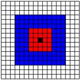
Figure 1. The Moore neighborhood template

2.6

The transition rule will be discussed in section 3.

Description of the behavior and the characteristics of the organization members and the environment

Behavior

2.7

In the work place people must work as part of a team in order to accomplish their personal and organizational goals. In order for this interdependence to work a degree of trust must exist between co-workers. The amount of trust that exists within an organization can be determined by how well workers can be observed relating to one another (Mayer, Davis & Schoorman 1995). According to this definition, trustor and trustee have the equal position, e.g., a party to another party, an employee to another employee. In this paper, the two parties involved in loyalty do not have the identical position. "Loyalty to group" is defined through relations of a party (the members) to another party (group). The state of the group is dictated by group culture.

2.8

For experimental purposes, "a group" can be defined as "life space" where any individual is subject to forces resulting from a variety of factors (Lewin 1951). The "life space" can be represented by a virtual magnetic platform analogous to a magnetic field in physics. The core of the platform exerts force (i.e. gravity) upon each member of the group. Here gravity represents group culture while its pull represents the "pull" of behavior to the "force" of group culture. This demonstrates that members can be expected to behave amenably to the core culture of the group — and the more amenable a member is, the higher his loyalty to the group.

2.9

CA is used to measure degree of loyalty as defined above. The lattices of CA are redefined here according to the properties of "life space". Each cell, or group member, indicates the member's degree of loyalty. The center cell represents the core culture of the group. The distance between any one cell and the center cell denotes its degree of loyalty. Simulation demonstrates the center cells "pull" on all other cells thus simulating the "pull" of group culture upon group members. The closer a member is to the center cell, the greater their loyalty. CA demonstrates that members will gravitate to the center.

2.10

Following these principles as outlined above, loyalty is measured according to the following three guidelines:

1. Degrees of loyalty are generalized into three values: "high", "normal" and "low". As illustrated by Figure 2, the black center cell on the lattice denotes the highest loyalty value (Figure 2). Red cells denote a "high" degree of loyalty, blue denotes "normal", and the white area represents those whose loyalty is "low".
2. Each cell represents one group member. So, if a member is represented by a "red" cell, then this member's loyalty is considered "high".

   Figure 2. The distribution of loyalty values

3. A group is composed of two parts: a formal sub-group and an informal sub-group. As was discussed in section 2.1, formal members dominate and tend to be the most loyal as long as external and internal factors have not changed. Thus, initially, the degree of loyalty attributed to formal members is "high". The degree of loyalty of members will evolve with simulation runs.

Individual Characteristics and Motives

2.11

A group, structurally speaking, can be divided into two groups (as outlined above). From here a group can be divided further according to two generalized sets of characteristics, and which result in differing motivations: One group being "economic", and the other being "social". According to the theory on employee behaviors" (Robbins et al 1997), Economic Beings are motivated by material and monetary gains. Social Beings are motivated by social status and the respect of their colleagues.

2.12

Motivation is mapped upon a function. We use stochastic variable X_i with uniform distribution to represent characteristic of member i, as shown graphically in Figure 3. Thus, X_i is the probability density function of characteristic of member i.

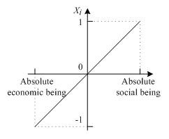
Figure 3. Function of member's characteristic

2.13

In this paper, we generalize the degree to which a categorization applies (as a social or economic motivation) as either "absolute" or "normal". If, for example, a member is identified as an "absolute economic being" this indicates the member is motivated by monetary rewards only. His behavior therefore can only be influenced by the implementation of an economic policy. If, however, a member is identified as a "normal economic being", this indicates that the member is mostly interested in monetary rewards, but not exclusively. His behavior therefore will be influenced most by economic policies while, to a lesser extent, will also be influenced by social policies. An "absolute social being" will behave in the exact opposite way. This member is motivated by social rewards only and therefore can only be influenced by the offer of a social policy.

Environmental factors

2.14

Environmental factors that influence behavior can be divided into two sub-groups: the internal and the external. Managerial policy (i.e. incentives), an internal factor, will be the factor used for the experimental purposes of this paper. Policies exist to address concerns that can be represented generally by one of two categories: Economic and Social. If management looking to motivate employees does so by offering a policy effecting income, then the policy is considered Economic in nature. If management implements a new training program or policy relating to the organizational culture of the workplace, then this policy is Social in nature.

2.15

Let EF be the degree of a new managerial policy (i.e. incentive). EF is illustrated graphically in Figure 4. EF is the probability density function of the new policy. As mentioned above, a policy can be classified as either "absolute" or "normal". An economic policy that is characterized as "absolute" is strictly economic without any social implications at all. A "normal" classification characterizes a policy as being mostly economic while including some social implications as well.

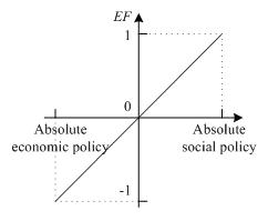
Figure 4. Function of a managerial policy

The CA based QSIM method

The rules

Rule 1: generating the initial behavior state

3.1

Initially, members of the two sub-groups are located on different parts of the lattice (Figure 2), indicating that their initial degree of loyalty differs. According to the principles outlined above (section 2.3 and 2.7) members are placed according to the following rules:

• Formal member loyalty must initially be greater than informal member loyalty.
• A cell can not represent more than one member. Two or more members cannot occupy a single cell.
• Formal members will tend to be more cohesive than informal members, since informal members tend to be more independent.

3.2

For example; the loyalty of formal members is initially considered "normal". They gravitate towards the center (See Figure 5) and are therefore located within the blue area of the lattice. Informal members, on the other hand, are initially represented within the white area since they tend to gravitate away from the center.

Rule 2: transition

3.3

There are two important transitions indicated by Figure 5 (a) and (b). The black center cell on the lattice denotes the highest degree of loyalty possible. The black ring denotes actual member loyalty.

3.4

Environmental factors influence member loyalty. When there is a change in the environment (a new policy) the degree of loyalty amongst group members will also changed. The result is a transition from one behavior state to another as illustrated below (Figure 5). As you can see, each member has moved from one cell to another.

(a)	(b)
Figure 5. Transition of a member's loyalty value on the lattice

3.5

According to section 2.7, the closer a member is to the center, the greater the degree of loyalty. The cause and effect relationship between a policy and loyalty is denoted as W. Where, W = <->, <0> or <+ >. "-" indicates the policy has effected member loyalty negatively, "0" indicates no effect at all and "+" indicates an effect that is positive. So; the placement of the black ring following the change in policy is determined by W:

3.6

If W = "-", then the black ring will move to a cell that is further from the center as indicated by the blue rings in Figure 5(a) and (b).

3.7

If W = "0", then the black ring will move to a cell whose distance from the center is equal to it's initial placement as indicated by the gray rings and the black ring itself in Figure 5(a) and (b).

3.8

If W = "+", then the black ring will move to a cell that is closer to the center as indicated by the red rings in Figure 5(a) and (b).

3.9

A black ring in transition must occupy a neighboring cell. If the neighboring cell is already occupied, the black ring will remain in it's initial position.

Filter

3.10

According to Rule 2, there must be more than one transition at each time stage. The number of transitions possible in Figure 5 is listed below (Table 1) with differing values for W.

Table 1: The number of possible transitions in Figure 5
W	-		0		+
Figure 5	(a)	(b)	(a)	(b)	(a)	(b)
Number of transitions	3	4	3	2	3	3

3.11

Each transition results in a new successor behavior state for a member. This change in successor states results in various combinations.

3.12

There are multiple successor states which will occur at the onset of each new time stage, many of which will be so unlikely that they will not be worth taking into consideration. These anomalies will be filtered according to what hitherto will be referred to as the "Loyalty-cost equilibrium".

The Loyalty-Cost Equilibrium

3.13

As discussed in section 2.7, a group functions like a magnetic field (Lewin 1951;Hayakawa 2000) which pulls on those located within the field. This "pull" refers to the organizational culture. Motivated by a desire for status and respect (Blau 1964), group members are drawn by the culture to behave loyally to their group. We will refer to this force hitherto as loyalty gravitation. This force, however, can be counteracted by motivations relating exclusively to the individual (Prien, Rasheed and Kotulic 1995). As discussed in section 2.1, group members will evaluate the cost and benefits of being loyal to their group against those of behaving according their own self interest. Having done so may influence members to gravitate away from behaving loyally. We will refer to this force hitherto as cost gravitation.

3.14

Loyalty gravitation is the draw to behave according to the best interests of the group while cost gravitation is the draw to behave according to the best interests of the self. When the environment has not changed (At the initial time stage, for example) the group is considered "settled" into a state of "normality". This state is the point of equilibrium: The loyalty gravitation and cost gravitation amongst group members is equal.

3.15

When something new is introduced, like a change in policy, the environment changes which therefore changes the group. Group members begin evaluating the costs and benefits of behaving loyally vs. behaving selfishly. This generally results in an overall oscillation between the two behaviors. If members are able to behave loyally with minimal personal sacrifice, then another loyalty-cost equilibrium is achieved. After a period of oscillation, the group becomes accustomed to the new environment. When a state of equilibrium such as this has been achieved, the difference between loyalty gravitation and cost gravitation is equal or near to zero.

Calculation of loyalty gravitation versus cost gravitation

3.16

Here we will calculate the pull of these two forces on a single group member. The force of this pull will be represented as distance from the center on the lattice below (Figure 6). The value (force) of the pull is determined by the distance between the ring (member) and the cell in the center (absolute loyalty).

3.17

Let D_i(t) represent the loyalty gravitation of member i at time stage t. Figure 6 will illustrate this calculation. Suppose that the cell and ring in Figure 6 illustrate the highest loyalty value of the group and of member i at time stage t, respectively. Figure 6(a) D_i(t) then calculates as follows:

Di ( t) = 2

3.18

In Figure 6(b) a right-angled triangle is formed, Di(t) is calculated as:

Di ( t) = √ 12 + 22

(a)	(b)
Figure 6. Calculating the distance between cells

3.19

Let C_i(t) be the cost gravitation of member i at time stage t. As discussed above, the group is in a state of equilibrium at the initial time stage (t = 0). Therefore, we specify:

Ci (0) = Di (0)

(1)

Following the initial time stage, the interaction between environmental changes and the characteristics of group members can be expected to change D_i(t) or C_i(t) correspondingly.

Calculation of W

3.20

Calculation of the loyalty-cost equilibrium is according to the following: When loyalty gravitation is less than or greater than cost gravitation, then W = "-" or "+" respectively. When they are equal, W = "0". The value of W is calculated as thus:

e(t) = Di(t) - Ci(t)

(2)

where e(t) is the difference between loyalty gravitation and cost gravitation of member i at time stage t. If e(t) < 0, then W= "-". If e(t) = 0, then W= "0". If e(t) > 0, then W= "+". Therefore, at initial time stage (i.e. t = 0), W= "0". When an environmental change occurs at the initial time stage, the resulting change D_i(t) or C_i(t), indicating W ≠ "0" and that, therefore, the black ring will move.

3.21

Let α _i and β _i be the change value of C_i(t) and D_i(t), respectively. These are caused by the interaction between an environmental change with the characteristics of group members. C_i(t+1) and D_i(t+1) are calculated as follows:

Ci(t+1) = Ci(t) + αi

(3)

Di(t+1) = Di(t) + βi

(4)

where α _i, β _i ∈[-1,1].

3.22

In simulation runs, the result of this interaction is determined by multiplying the characteristics of group members (X_i) by the new policy (EF). These calculations are expressed as α _i and β _i and listed in Table 2.

Table 2: Calculation of α i and β i
Sub-group	Characteristic of member	Economic policy	Social policy
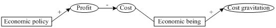
Formal sub-group or Informal sub-group	Economic being	α i = -Xi·EF (5)	β i = 0.5·EF (7)
	Social being	α i = 0.5·EF (6)	β i = Xi·EF (8)

3.23

The above calculation is appropriate for every group member regardless of whether he/she is in the formal or informal sub-group. The formation of Table 2 is clarified by examining Figure 7.

(a) Formation of Equation 5

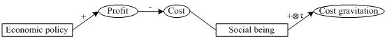
(b) Formation of Equation 6

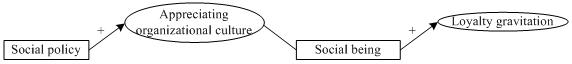(c) Formation of Equation 8

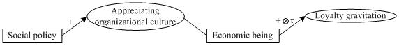(d) Formation of Equation 7

Figure 7. Causality of management policy, characteristic of member and the gravitations

3.24

According to Figure 7(a) and (b), the economic policy (EF) has a positive effect ("+") (i.e. an increase in profit) on the member, since an increase in EF means an increase in profit. An increase in profit means, by extension, a negative effect ("-") on his cost, since an increase in profit means a corresponding decrease in cost. This decrease will have a positive effect on his cost gravitation; if his cost decreases, then cost gravitation for him will decrease accordingly. The degree, however, of the positive effect will differ according to the differing characteristics between individual members. For an economic being, the degree of the positive effect is normal (see Figure 7a) since economic gain is his primary motivation. A social being, on the other hand, is uninterested in economic gain, and so the positive effect should be decreased to a percent of τ (see Figure 7b). In this paper we indicate that τ =50%.

3.25

In Figure 7(c) and (d), a social policy change (EF) will positively effect the loyalty gravitation ("+") of members who are motivated by changes in the organizational culture. The degree, however, of this positive effect will depend on the differing characteristics of individual members. For a social being the degree of positive effect is normal (see Figure 7c) since social gain is his primary motivation. An economic being, on the other hand, is uninterested in social gain and so the positive effect should be decreased to a percent of τ (see Figure 7d, τ =50%).

Filter theory

3.26

Let D(t) and C(t) express the average loyalty gravitation and cost gravitation of the group overall at time stage t, respectively. They are calculated as thus:

(9)

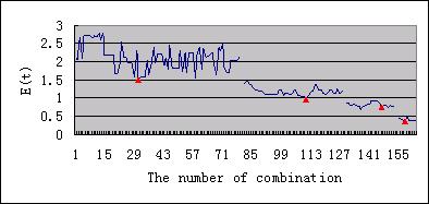
where n is the number of members in the group. Let E(t) = | D(t)- C(t)|. Here the filter functions as follows: At each time stage t the lowest combinations E(t) are kept. All remaining combinations are disregarded.

Simulation engine

3.27

A simulation engine is used to integrate all the above components and to drive simulation runs.

3.28

Setup work:

• Specify the number of formal members and informal members, n;
• Define X_i, (the characteristic of member i), i=1, 2, ..., n; and
• Determine EI or SI

3.29

The simulation engine runs as follows:

• Step 1: Generate the initial state for all members by applying Rule 1.
• Step 2: Move all members simultaneously by applying Rule 2, let t = t +1.
• Step 3: Calculate C(t) and D(t) using equations 3 and 4.
• Step 4: Filter anomalous successor states by applying the Filter.
• Step 5: If E(t+1) >= E(t), then the simulation ends. Otherwise, continue.
• Step 6: Determine the value of W by Equation 2 and then go back to Step 2.

Qualitative Validation

Conceptual model and its validation steps

4.1

The above components can now be integrated to form a conceptual model of the CA based qualitative simulation of group behavior. The framework for this model is illustrated below (Figure 8).

4.2

The first component is the description method. Based on it, values are assigned according to the characteristics of group members. An environmental change is input and the rules are triggered. The third component, the filter, is run, and then the fourth component, the qualitative simulation engine, drives runs of all these components combined.

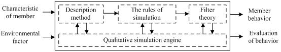
Figure 8. Conceptual model of CA based qualitative simulation with inputs and outputs

4.3

The characteristics of group members and environmental changes are factored into the conceptual model according the following:

• n₁ and n₂, i.e., the number of formal members and informal members;
• X_i, i.e., characteristic of member i, i=1, 2, ..., n₁ + n₂; and
• EF, i.e., new managerial policy.

4.4

Member behavior and the evaluation of this behavior is output from the conceptual model as follows:

• Cell formations on the lattice, i.e., member behaviors at each time stage;
• D(t), i.e., total loyalty gravitation of the group at time stage t; and
• E(t), i.e., marginal absolute difference between loyalty gravitation and cost gravitation.

4.5

The two latter indexes are used to evaluate member behavior. D(t) represents the group's loyalty value at each time stage, while E(t) is used to evaluate simulation runs in oscillation-equilibrium mode.

4.6

In this section, we discuss the validity of the CA based qualitative simulation. As stated in Dijkum et al (1999), methods of validation are classified into two types: quantitative (or basic) validation and qualitative validation. For our purposes the qualitative method is clearly the most appropriate. There is no full-proof method for determining the validity of qualitative simulation. We can, however, conduct a reasonable assessment via the following:

First: Isolate an example.
Second: Design a sampling of varying inputs, each a differing combination of member characteristics and a change of policies.
Third: Run a simulation of each to yield a corresponding output.
Fourth: Assess process of input to output according to common managerial sense. If these are consistent, then the proposed method is valid. Otherwise it is not.

4.7

Output here are cell formations and E(t). The cell formations are consistent with common sense. E(t) will demonstrate the "oscillation-equilibrium" that is characteristic of the proposed method.

Example of a group and designs for experimentation

4.8

A group is comprised of two sub-groups, formal and informal. The formal sub-group contains twenty members; the informal sub-group contains ten. A value is assigned to the characteristics of members within each sub-group according to the distribution of economic vs. social beings within each. The environmental factor for our purposes is a new managerial policy. A value is assigned to this policy according to the degree by which it can be considered economic or social. Using a sampling of policies that vary in degree either way, we demonstrate that transitions in group behavior vary accordingly. For the purposes of this paper the specific behavior in question is group loyalty.

4.9

Three factors are input for experimentation: The characteristics of formal members, the characteristics of informal members, and a new managerial policy. In order to generate an output from the conceptual model that can readily be identified as valid or not, we will input extreme cases (absolutes) only. Eight experimental combinations are run as seen in Table 3.

Table 3: Experimental designs
Experimental runs (first to last)	1	2	3	4	5	6	7	8
Characteristic of formal members	EB	EB	EB	EB	SB	SB	SB	SB
Characteristic of informal members	EB	EB	SB	SB	EB	EB	SB	SB
Managerial policy	EP	SP	EP	SP	EP	SP	EP	SP

where EB is an absolute economic being, SB is an absolute social being, EP is an absolute economic policy and SP is an absolute social policy.

Qualitative simulation and analysis

4.10

We use Visual Basic 6.0 to code the CA based qualitative simulation. Its interface is shown in Figure 9.

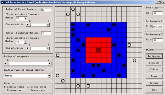
Figure 9. Initial behavior state of the group (on the lattice)

4.11

On the left side of the screen is the "input window". Here we key in the number of formal and informal members (20 and 10), the value of each member characteristic (EB or SB) and the value of the managerial policy (EP or SP). The initial behavior state of formal members is specified as "normal". The center screen shows cell formation at each time stage. The field on the upper right-hand side indicates which time stage is currently on screen, and the two fields below it evaluate the current cell formation. The buttons below are for running simulations.

4.12

Once all values have been keyed in, clicking "Initialize" will generate the initial behavior state onto the lattice. The dark red cell in the center represents the highest degree of loyalty possible. The cells containing black dots show the loyalty value of formal members while cells containing black rings show the loyalty value of informal members. Since we designate the initial behavior state of formal members as "normal", those members (the black dots) all crowd within the blue area of the lattice while informal members (the black rings) scatter across the grey.

4.13

Clicking "Simulate" will generate a cell formation for one time stage according to values entered on the left, and then, will advance through subsequent time stages generating a different cell formation for each as values (behaviors) change. Black dots and rings on the lattice will appear to be moving. Once the simulation has stopped, clicking "Filter" will filter out anomalies according to the theory of loyalty-cost equilibrium thus establishing the most likely combination of behaviors at each time stage. These combinations can then be browsed by clicking "Browser".

4.14

The following are the results of simulation at the last time stage of the eight experimental combinations specified in Table 3.

Figure 10. Simulation result with experimental design 1

4.15

In Figure 10, all members (formal and informal) are absolute economic beings while the new policy is absolute and economic as well. In this case, all dots and rings (representing member behavior) move quickly and much closer to the center cell on the lattice. This indicates that degree of loyalty for all members will greatly increase.

Figure 11. Simulation result with experimental design 2

4.16

In Figure 11, all members are absolute economic beings while the new policy is absolute and social. In this case, the dots and rings move towards the center, but only slightly. This indicates that group loyalty for all members will increase only slightly.

Figure 12. Simulation result with experimental design 3

4.17

In Figure 12, formal members are absolute economic beings, informal members are absolute social beings, and the policy is an absolute economic policy. In this case, the dots move much closer to the center cell, while the rings move only slightly. This indicates that loyalty amongst formal members greatly increases while loyalty amongst informal members increases only slightly.

Figure 13. Simulation result with experimental design 4

4.18

In Figure 13, formal members are absolute economic beings, informal members are absolute social beings, and the policy is an absolute social policy. In this case, the dots move toward the center cell, but only slightly, while the rings move much closer. This indicates that loyalty amongst formal members changes only slightly while loyalty amongst informal members increases greatly.

Figure 14. Simulation result with experimental design 5

4.19

In Figure 14, formal members are absolute social beings, informal members are absolute economic beings, and the policy is an absolute economic policy. In this case, the dots do not move to a degree worth noting. The rings do move closer to the center, but only slightly. This indicates that loyalty amongst formal members does not change, while loyalty amongst informal members does, but only slightly.

Figure 15. Simulation result under experimental design 6

4.20

In Figure 15, formal members are absolute social beings, informal members are absolute economic beings, and the policy is an absolute social policy. In this case, the dots move much closer to the center cell. The Rings move only slightly. This indicates that loyalty amongst formal members greatly increases, while loyalty amongst informal members increases only slightly.

Figure 16. Simulation result under experimental design 7

4.21

In Figure 16, all group members are absolute social beings while the new policy is an absolute economic policy. In this case neither the dots nor the rings move.

Figure 17. Simulation result under experimental design 8

4.22

In Figure 17, all group members are absolute social beings while the policy is an absolute social policy. In this case, all dots and rings move much closer to the center. This indicates that loyalty amongst all members has greatly increased.

4.23

The value of E(t) at each time stage for all eight experimental designs are illustrated by figures 18 through 25. The red triangles represent the lowest value of E(t) at each time stage.

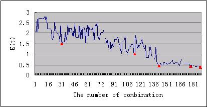
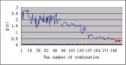
Figure 18. E(t) of experimental design 1

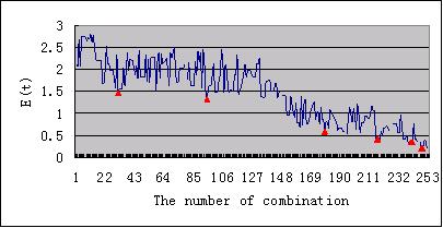
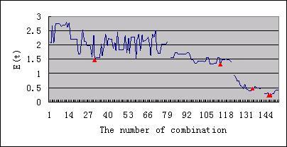
Figure 19. E(t) of experimental design 2

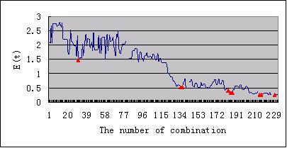
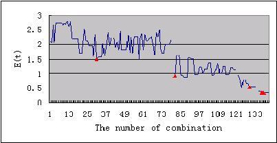
Figure 20. E(t) of experimental design 3

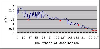
Figure 21. E(t) of experimental design 4

Figure 22. E(t) of experimental design 5

Figure 23. E(t) of experimental design 6

Figure 24. E(t) of experimental design 7

Figure 25. E(t) of experimental design 8

4.24

The above simulation results are consistent with what common sense readily identifies as valid. Let us break down a few examples in order to demonstrate this further: Figure 10 illustrates a case where group members — both formal and informal — are motivated by monetary rewards only. If a manager looking to motivate group loyalty amongst this particular group implements a new policy that is economic in nature, he or she will certainly be successful. Figure 11 illustrates a case where a manager attempts to motivate group loyalty amongst the same group (all motivated by monetary gain) by implementing a new policy that is social. Group loyalty in this case may increase, but only slightly. Figure 12 illustrates a case where formal members are motivated by monetary rewards while informal group members are motivated by rewards that are social. If management implements a new policy in this case that is economic, the loyalty of formal members will greatly increase while the loyalty of informal members can be expected to increase only slightly. Figure 13 illustrates a case involving the same group as illustrated in Figure 12, only this time the policy is social rather than economic. The result therefore is the opposite of Figure 12; formal members are motivated very little, whereas informal members are greatly motivated and, thus, loyalty amongst them increases greatly. Figure 14 illustrates a case where formal members are motivated socially, while informal members are motivated monetarily. The policy offered is economic, and thus; Loyalty amongst formal members of the group is affected little while loyalty amongst informal members greatly increases. Figure 15 illustrates a case where formal members are motivated by social rewards while informal members are motivated by monetary rewards. The implementation of a social policy in this case means loyalty amongst formal members increases greatly while loyalty amongst informal members increases very little. Figure 16 illustrates a case where all members are motivated by social rewards. The new policy here is an economic policy and, as such, loyalty amongst members is affected very little. Figure 17 illustrates a case that, in simulation, is identical to that in Figure 1. All group members are motivated by the same (in this case social rewards) and because the new policy caters to what motivates the group (in this case, a social policy) group loyalty amongst all group members greatly increases.

4.25

The eight experimental simulations as detailed above, followed by an analysis of results, demonstrates the following:

• Simulation results are always consistent with what common sense accepts as valid.
• Simulation runs show oscillation-equilibrium between time stages; and
• The Loyalty-cost equilibrium is gradually achieved through simulation runs.

4.26

An assessment of these simulation results and corresponding statistics ( E(t)) allows us to reasonably conclude that the CA based qualitative simulation method is valid.

Application of the proposed method to decision making

5.1

Table 4 (below) presents the details of a case study which demonstrates how the CA based qualitative simulation can be applied to decision making.

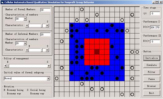
Table 4: A case of a group
Formal sub-group	Number of members	30
	Characteristic of members	Normal economic being, 15 Normal social being, 15
Informal sub-group	Number of members	20
	Characteristic of members	Normal economic being, 10 Normal social being, 10

5.2

The question we ask for the purposes of this study is this: Which policy would most effectively motivate group members to behave more loyally? According to section 3.27 there are four alternative policies to choose from:

• Alternative 1: absolute economic
• Alternative 2: normal economic
• Alternative 3: normal social
• Alternative 4: absolute social

5.3

Where a company stands financially may directly effect which policy management chooses to implement. It is possible that, at the initial time stage, a new economic policy is not financially viable, and thus, only social policies are available.

5.4

We will run four simulations as proposed, one for each possible policy. We will then decide, based on these results, which policy is likely to be most effective.

5.5

The group's initial behavior state is randomly generated onto the lattice as shown below (Figure 26). The result of simulation at the last time stage for all four policies is also shown below (Figure 27).

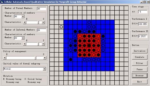
Figure 26. The initial behavior state of the group

(a) Alternative 1

(b) Alternative 2

(c) Alternative 3

(d) Alternative 4

Figure 27. Simulation results at the last time stage

5.6

At the last time stage, D(t) simulation results for the four types of policy — 1, 2, 3 and 4 — are 164.168, 139.541, 134.926 and 157.559, respectively.

5.7

As discussed in section 4.8, D(t) represents the groups overall loyalty gravitation. Since this value is determined by the distance between cells (group members) and the center cell (greatest loyalty value possible), it therefore also represents the group's overall loyalty value. This representation, however, occurs in terms that are opposing. If the Loyalty gravitation D(t) of a group is low, this indicates that the space between cells and the center on the lattice is small, which therefore also indicates that the loyalty value is high.

5.8

Simulation results indicate that Alternative 2 and 3 are more effective motivators than Alternative 1 and 4. This can also been seen visually by comparing the cell formations on the lattice for each Alternative in Figure 27. The black dots and rings gather closer to the center in Figure 27(b) and 27(c) than those in Figure 27(a) and 27(d).

5.9

At this point the better of the two outstanding policies can not be distinguished, since simulation results for both at the last time stage are almost the same. To do this we will need to take behavior at previous time stages into consideration as well. Below (Figure 28 and Figure 29) are the results of simulation at all time stages for Alternative 2 and 3, respectively.

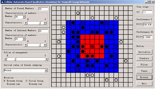
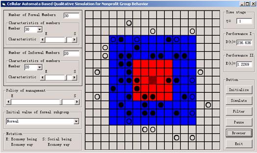
(a) at time stage t = 1

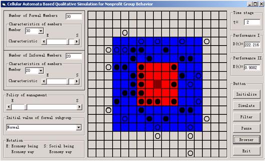
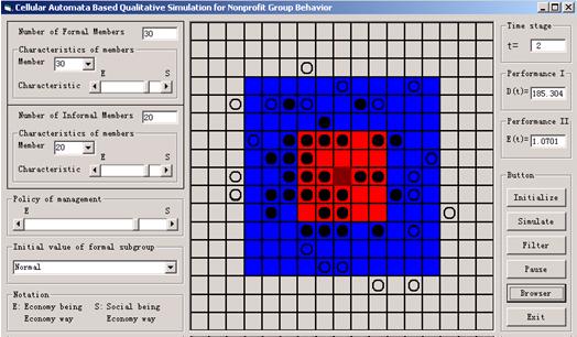
(b) at time stage t = 2

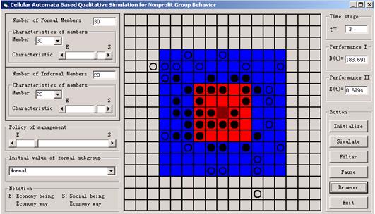
(c) at time stage t = 3

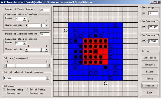
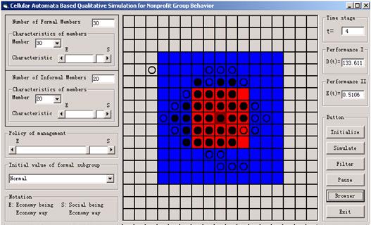
(d) at time stage t = 4

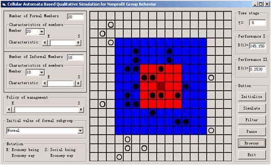
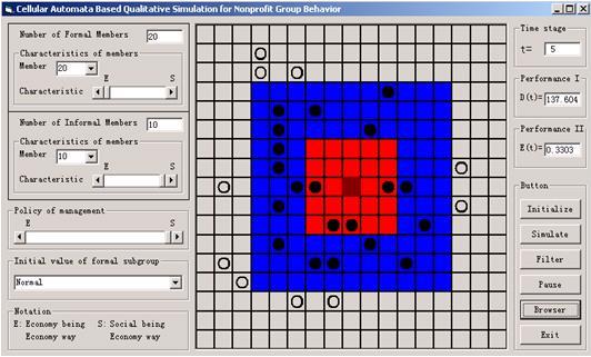
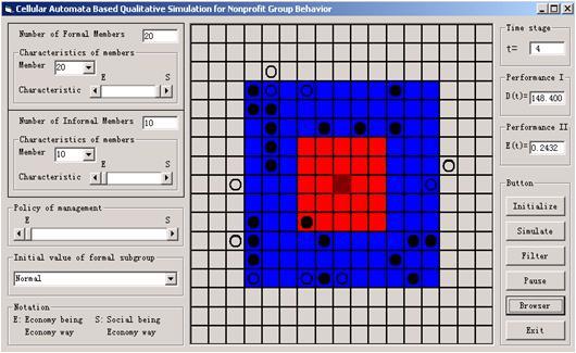
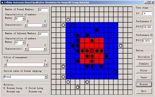
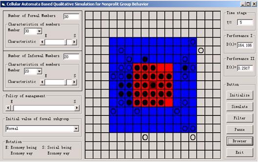
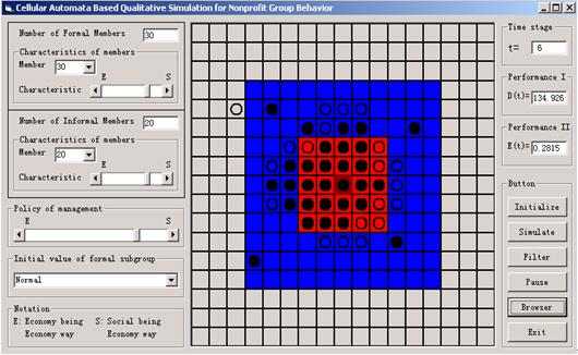
Figure 28. Simulation results for Alternative 2

(a) at time stage t = 1

(b) at time stage t = 2

(c) at time stage t = 3

(d) at time stage t = 4

(e) at time stage t = 5

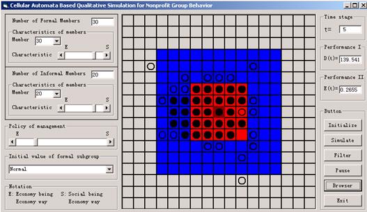
Figure 29. Simulation results for Alternative 3

5.10

Figure 30 shows graphically the result (D(t)) of simulation runs for Alternative 2 and 3. The black line represents the D(t) for Alternative 2 while the red line represents Alternative 3.

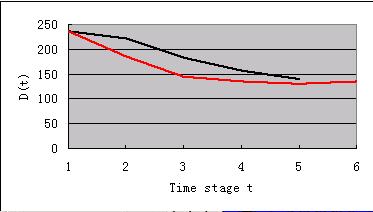
Figure 30. D(t)of Alternative 2 and 3 with simulation runs

5.11

Alternative 2 and 3 are compared as follows:

• Loyalty value: The Loyalty value resulting from Alternative 2 is greater than that from Alternative 3 at every time stage.
• Duration: The duration of the simulation runs (the number of time stages required to re-establish equilibrium) for Alternative 2 is shorter than for Alternative 3 (five and six time stages respectively). This indicates that oscillation will stop (things will go back to "normal") sooner subsequent to Alternative 2 than it will subsequent to Alternative 3.
• Consistency: The simulation run for Alternative 3 indicates a decrease in loyalty value at time stage t = 6. Group behavior is therefore not as consistent following Alternative 3 as it is following Alternative 2.

5.12

Taking duration into principle consideration designates a normal economic policy (Alternative 2) would be the most efficient. The Loyalty value, however, resulting from a normal social policy (Alternative 3) is always greater than that resulting from Alternative 2 — instability notwithstanding — and since an increase in loyalty value is our primary goal we conclude that a normal social policy would be a better choice than a normal economic policy.

Conclusions and further work

6.1

Variation in behavior amongst group members is an important reason why managerial science is so complex. The qualitative simulation approach for the study and prediction of group behavior should be the first of computer simulation techniques considered for managerial use. The most well known qualitative simulation method QSIM, which was originally designed for the study of physical systems, is inappropriate for the study of group behavior. We have, therefore, proposed the use of QSIM in combination with CA modeling. Some components of QSIM (the generation of successor states, the filtering of anomalies, and the simulation engine) have been retained while CA modeling has been added for results that are clearer and more precise. The integration of QSIM and CA modeling is the basis of CA based qualitative simulation.

6.2

We have also designed a filter for behavioral anomalies based upon the concept of "loyalty-cost equilibrium". Loyalty gravitation and cost gravitation amongst members is calculated and then filtered based upon common sense and an understanding of managerial science.

6.3

We use Visual Basic 6.0 to code our proposed method. To test the validity of our method, we conduct experiments designed using extreme examples. These examples allow for results which readily be identified as valid or invalid. These experimental simulation runs demonstrate clearly that our proposed method is valid.

6.4

The validity of this method is demonstrated further by a case study where a decision regarding a policy and its effect on group behavior must be made, and to which the CA based QSIM is applied. By conducting simulation runs for each of four possibilities, we obtain results allowing for an analysis of values (i.e. loyalty value) at each time stage, thus allowing managers a more informed decision than would be possible otherwise.

6.5

Further research for this paper includes study of the following:

1. CA based qualitative simulation for general organization. A group is the most basic organizational unit whose members are subject primarily to social rather than physical considerations. A group of employees, however, is more complicated. Groups interacting in the workplace involve hierarchies' and economic interdependence rendering their interaction with one other and with their environment unique and especially complex.
2. CA based description method for a set of behavior. For the purpose served by this paper CA is employed for study of a single behavior only (i.e. group loyalty). In reality, however, behaviors should be studied in combination since individual behaviors are not mutually exclusive.

Acknowledgements

Our work was conducted as part of the Qualitative Simulation Team Work for Complex Management Systems at Modernized Management Institute, School of Management, Huazhong University of Science and Technology. Our study of Qualitative Simulation Team Work for Complex Management Systems was supported by the China National Natural Science Fund (No.70271029 and No. 70671048), and the China Hubei Province Natural Science Fund (No. 2004ABA069). The authors would like to thank the anonymous referees for their comments and suggestions on early versions of this paper.

References

BERENDS P, Romme G (1999) Simulation as a Research Tool in Management Studies. European Management Journal, 17(6). pp.576-583

BLAU P (1964) Exchange and Power in Social Life. Transaction Publishers, New Brunswick

CONTE R, Paolucci M (2002) Reputation in artificial societies: Social beliefs for social order, Norwell: Kluwer Academic Publishers

DIJKUM C, Detombe D and Kuijk E (1999) Validation of Simulation Models. Amsterdam: SISWO (SISWO Publication 403)

FRANK K A, Yasumoto J Y (1998) Linking action to social structure within a system: Social capital within and between subgroups. American Journal of Sociology, 104(3). pp. 642-686

HAYAKAWA H (2000) Bounded rationality, social and cultural norms, and interdependence via reference groups. Journal of Economic Behavior & Organization, 43. pp.1-34

HEGSELMANN R and Flache A (1998) Understanding Complex Social Dynamics: A Plea For Cellular-automata Based Modelling. Journal of Artificial Societies and Social Simulation, 3(1) https://www.jasss.org/1/3/1.html

JANSSEN M and Jager W (1999) An integrated approach to simulating behavioural processes: A case study of the lock-in of consumption patterns. Journal of Artificial Societies and Social Simulation, 2(2) https://www.jasss.org/2/2/2.html

KLÜVER J and Stoica C (2003) Simulations of Group Dynamics with Different Models. Journal of Artificial Societies and Social Simulation, 6(4) https://www.jasss.org/6/4/8.html

KUIPERS B (1986) Qualitative Simulation. Artificial Intelligence, 29. pp. 289-338

LEWIN K (1951) Field theory in social science. New York: Harper

MAYER, Davis & Schoorman (1999) An integrative model of organizational trust, Academy of Management Review, 20(3). pp. 709-734

PRIEN R L, Rasheed A, Kotulic A G (1995) Rationality in Strategic Decision Processes, Environmental Dynamism and Firm Performance. Journal of Management, 21(5). pp. 913-929

ROBBINS S, Coulter M, Stuart-Kotze R (1997) Management. Ontario: Prentice Hall Canada

VALLACHER R R, Nowak A (1994) Dynamical Systems in Social Psychology, CA: Academic Press

VALLACHER R R, Nowak A (1997) The Emergence of Dynamical Social Psychology. Psychological Inquiry, 8(2). pp. 73-99

Return to Contents of this issue

© Copyright Journal of Artificial Societies and Social Simulation, [2006]