Paul Windrum, Giorgio Fagiolo and Alessio Moneta: Empirical Validation of Agent-Based Models

©Copyright JASSS

Paul Windrum, Giorgio Fagiolo and Alessio Moneta (2007)

Empirical Validation of Agent-Based Models: Alternatives and Prospects

Journal of Artificial Societies and Social Simulation vol. 10, no. 2, 8
<https://www.jasss.org/10/2/8.html>

For information about citing this article, click here

Received: 22-May-2006 Accepted: 08-Jan-2007 Published: 31-Mar-2007

Abstract

: This paper addresses a set of methodological problems arising in the empirical validation of agent-based (AB) economics models and discusses how these are currently being tackled. These problems are generic for all those engaged in AB modelling, not just economists. The discussion is therefore of direct relevance to JASSS readers. The paper has two objectives. The first objective is the identification of a set of issues that are common to all modellers engaged in empirical validation. This gives rise to a novel taxonomy that captures the relevant dimensions along which AB modellers differ. The second objective is a focused discussion of three alternative methodological approaches being developed in AB economics — indirect calibration, the Werker-Brenner approach, and the history-friendly approach — and a set of (as yet) unresolved issues for empirical validation that require future research.
Keywords:: Methodology, Empirical Validation, Agent-Based Models, Simulation, Calibration, History-Friendly Models

Introduction

1.1

This paper identifies a set of fundamental validation problems faced by all those engaged in agent-based (AB) economics, and assesses the strengths and weaknesses of alternative empirical validation procedures that have been developed in recent years. The paper locates the problems, and proposed solutions, within 3 domains: (1) the relationship between theory and empirical research, (2) the relationship between models and the real-world systems being modelled, and (3) the way in which a validation procedure deals with (1) and (2). These issues are generic and apply to all those engaged in AB modelling. The discussion in this paper is therefore highly relevant to JASSS readers.

1.2

Before proceeding, let us define what is meant by AB models^[1]. These tend to contain the following three ingredients.

Bottom-up perspective. The properties of macro-dynamics can only be properly understood as the outcome of micro-dynamics involving basic entities/ agents (cf. Tesfatsion 2002). This contrasts with the top-down nature of traditional neoclassical models, where the bottom level typically comprises a representative individual and is constrained by strong consistency requirements associated with equilibrium and hyper-rationality. Conversely, AB models describe strongly heterogeneous agents living in complex systems that evolve through time (Kirman 1997a; 1997b). Therefore, aggregate properties are interpreted as emerging out of repeated interactions among simple entities rather than from the consistency requirements of rationality and equilibrium imposed by the modeller (Dosi and Orsenigo 1994).
Boundedly-rational agents. Since the environment in which economic agents interact is too complex for hyper-rationality to be a viable simplifying assumption (Dosi et al. 2005), one can, at most, impute to agents in AB models some local and partial (both in time and space) principles of rationality, e.g. myopic optimisation rules. AB modellers maintain that socio-economic systems are inherently non-stationary, due to persistent novelty (e.g., new patterns of behaviour) endogenously introduced by the agents themselves. Hence, agents face 'true (Knightian) uncertainty' (Knight 1921) and are only able to partially form expectations, e.g. on technological outcomes. New technologies are introduced into open-ended technological spaces, and payoffs to R&D are non-static and cannot be known ex ante (Nelson and Winter 1982; Dosi 1988). As a consequence, agents face the extremely difficult task of learning and adapting in turbulent, endogenously changing, environments. On this basis, AB researchers argue that assumptions of individual hyper-rationality coupled with rational expectations are inappropriate starting points for modelling. Rather, agents should be assumed to behave as boundedly rational entities with adaptive expectations.
Networked direct interactions. Interactions among economic agents in AB models are direct and inherently non-linear (Fagiolo 1998; Windrum and Birchenhall 1998; Silverberg et al. 1988). Agents interact directly because current decisions directly depend, through adaptive expectations, on the past choices made by other agents in the population (i.e. a widespread presence of externalities). These may contain structures, such as subgroups of agents or local networks. In such structures, members of the population are in some sense closer to certain individuals in the socio-economic space than others. These interaction structures may themselves endogenously change over time, since agents can strategically decide with whom to interact according to the expected payoffs. When combined with heterogeneity and bounded rationality, it is likely that aggregation processes are non-trivial and, sometimes, generate the emergence of structurally new objects (Lane 1993a; 1993b).

1.3

A number of important consequences follow:

First, agents in AB models typically learn by engaging in an open-ended search of dynamically changing environments (Dosi et al 2005). Indeed, agents are not initially endowed with an understanding of the underlying structure of the environment in which they operate, but must develop a representation of its underlying structure. The introduction of endogenous novelty makes the task more difficult since the introduction of new objects alters this underlying structure and, hence, the payoffs associated with alternative actions. Furthermore, the complexity of the interactions between heterogeneous agents underpins open-ended search.
Second, partly as a consequence of adaptive expectations, AB models are characterised by true, non-reversible, dynamics, i.e. the state of the system evolves in a path-dependent manner (Marengo and Willinger 1997). The focus is on the self-organizing properties that emerge through these feedback loops. As Silverberg et al. (1988) observe, in economics we see "complex interdependent dynamical systems unfolding in historical, i.e. irreversible, time, economic agents, who make decisions today the correctness of which will only be revealed considerably later, are confronted with irreducible uncertainty and holistic interactions between each other and with aggregate variables" (Silverberg et al. 1988: 1036, italics in original).
Third, selection-based market mechanisms are sometimes at work in AB models (see, for instance, the model of technological change pioneered by Nelson and Winter 1982). Most obviously, the goods and services produced by competing firms are selected by consumers. The selection criteria that are used may themselves be complex and span a number of dimensions. Turbulence in industry dynamics can be created through successive rounds of firm entry and exit (Saviotti and Pyka 2004; Windrum and Birchenhall 2005; Windrum 2005).

1.4

AB researchers have enjoyed significant success over the last 20 years. Despite the deep philosophical differences that exist between AB and neoclassical models^[2], orthodox (neoclassical) economists have recognised the significance of the AB critique, and have reacted by extending their own modelling framework to incorporate (certain) aspects of heterogeneity, bounded rationality, learning, increasing returns, and technological change. Yet orthodox economists have not been moved to join the AB camp. There are many possible explanations for this but an important aspect, recognised by AB modellers themselves, is a perceived lack of robustness in AB modelling. This threatens the AB research enterprise as a whole. Four key problem areas were identified in a recent conference and special workshop attended by the authors^[3]. First, the neoclassical community has consistently developed a core set of theoretical models and applied these to a range of research areas. The AB community has not done this. Indeed, the sheer diversity of alternative AB models put forward over the last 20 years is striking.

1.5

A second, related set of issues concerns a lack of comparability between the models that have been developed. Not only do the models have different theoretical content but they seek to explain strikingly different phenomena. Where they do seek to explain similar phenomena, little or no in-depth research has been undertaken to compare and evaluate their relative explanatory performance. Rather, models are viewed in isolation from one another, and validation involves examining the extent to which the output traces generated by a particular model approximates one or more 'stylised facts' drawn from empirical research.

1.6

This leads us to a third issue: the lack of standard techniques for constructing and analysing AB models. It has been argued that developing a set of commonly accepted protocols for AB model building would benefit the profession (Leombruni 2002; Richiardi 2003). This would address, for instance, issues such as how and when sensitivity analysis (over the space of initial conditions and parameters) should be conducted, how one should deal with non-ergodicity in underlying stochastic processes, and how one should interpret, in terms of real-world time, the timing and lag structures that AB modellers typically build into their models.

1.7

Finally, the fourth set of issues concerns the problematic relationship between AB models and empirical data. Empirical validation of a model (M) involves an assessment of the extent to which M is a good representation of the (unknown) process that generated a set of observed data. This opens up a raft of fundamental questions. What is the methodological basis that informs the process of empirical validation? Is this process specific to AB models, or is it generic to all modelling enterprises? A central objective of this paper is the exploration of these issues.

1.8

As well as there being great diversity in the way AB modellers go about developing models, fundamental differences exist in the way they conduct empirical validation. Key areas of debate include whether a 'realist' methodology is appropriate? Why should empirical validation be the primary basis for accepting or rejecting a model? Do other forms of model validation exist besides the reproduction of stylised facts? If we do proceed down the path of empirical validation, then how should one relate and calibrate the construction of parameters, initial conditions, and stochastic variability in AB models to the existing empirical data? Which classes of empirically observed objects do we actually want to replicate? How dependable are the micro and macro stylised facts that are to be replicated? To what extent can we truly consider output traces to be stylised facts or, alternatively, counterfactuals? What are the consequences, for the explanative power of a model, if the stylised facts are actually 'unconditional objects' that only indicate properties of stationary distributions and, hence, do not provide information on the dynamics of the stochastic processes that generated them? Given these rather fundamental questions, it should not come as a surprise that very different approaches to empirical validation are found in the AB literature. A novel contribution of this paper is its explicit consideration of the basis for this heterogeneity.

1.9

The paper is structured as follows. Section 2 discusses the methodological basis of empirical validation, i.e. the comparison of discrete-time models with empirical data. The section begins with a discussion of the core issues of empirical validation faced by all modellers (neoclassical as well as AB economists). Having identified these core issues, section 3 opens the discussion on methodological diversity within the AB community. We suggest that this methodological heterogeneity is due to two factors. The first factor is the problem of modelling highly non-linear systems, i.e. systems with stochastic dynamics, non-trivial interactions among agents, and feedbacks from the micro to the macro level. The second factor is the diverse structural content of AB models, and the very different ways in which AB models are currently analysed. We present a novel taxonomy of AB models that captures the salient dimensions of this diversity. There are four dimensions: (1) the nature of the object under study, (2) the goal of the analysis, (3) the nature of the main modelling assumptions, and (4) the method of sensitivity analysis.

1.10

Building on section 3, section 4 provides a detailed survey of three major approaches to AB empirical validation. These are the indirect calibration approach (4.4), the Werker-Brenner approach to empirical calibration (4.10), and the history-friendly approach (4.18). We examine the strengths and weaknesses of each approach. This paves the way for a discussion, in section 5, of a set of unresolved issues for empirically-oriented AB modellers. Section 6 concludes.

The methodological bases of empirical validation: comparing discrete-time models with empirical data

2.1

In this section we clarify the process of empirical validation and identify a set of validation issues that are common to all modellers (neoclassical and AB alike). Let us consider the typical situation faced by any empirically-grounded economist attempting to replicate and/or explain a set of stylised facts. The point of departure is almost always a set of empirically observed data (e.g. panel data) whose generic form is:

(z)_i = { z_{i, t}, t = t ₀, …, t₁}, i ∈ I.

Here the set I refers to a population of agents (e.g. firms and households) whose behaviour has been observed across the finite set of time-periods {t₀, …, t₁} and refers to a list of, say, K variables contained in the vector z. Whenever agent-level observations are not available, the modeller has access to the K-vector of aggregate time-series:

Z = { Z_t, t = t ₀, …, ₁},

which can be obtained by summing up (or averaging out) the K micro-economic variables z_i,t, over i ∈ I. In both cases, the observed dataset(s) generate(s) a number of 'stylised facts' or statistical properties that the modeller is seeking to explain.

2.2

The datasets (z)_i, and/or Z are the unique outcome of an unknown, real-world data-generation process (rwDGP). Due to the impossibility of knowing the 'true' model of the world, we can think of the rwDGP as a very complicated, multi-parameter, stochastic process that governs the generation of a unique realisation that we can actually observe^[4]. The goal of the modeller is to provide a sufficiently good 'approximation' of the rwDGP in his/her model. The model will contain a simplified data-generation process, the model-DGP (mDGP). This mDGP should provide a meaningful explanation of the causal mechanisms that generate the observed stylised facts, as well as a good representation of the observed data. Therefore empirical validation is, in essence, is the process by which a modeller tries to evaluate the extent to which his/her mDGP is a good representation of the rwDGP^[5].

2.3

As mentioned, a set of methodological issues exist that concern all the natural and social sciences, and which remain the focus of intense debate in the philosophy of science. We have identified a set of core issues that relate to, and assist in explaining, different approaches to empirical validation found in discrete time-based economic modelling. Neither neoclassical economists nor AB modellers have precise or definite strategies on how to address these issues, but it is possible to assess important differences between the methodological strategies of the two approaches. We will deal with this task in the subsequent sections. First we need to identify and elucidate the core issues.

Concretisation vs. isolation. Faced with the essential complexity of the world, scientific (not just economic) models proceed by simplifying and focusing on relationships between a very limited number of variables. To start with, is it possible to model all the various elements of the rwDGP? How can we possibly 'know' all the different elements of the rwDGP? Economists usually agree that models should isolate some causal mechanisms, by abstracting from certain entities that may have an impact on the phenomenon under examination (see Gibbard and Varian 1978; Mäki 1992 and 2005; Janssen 1994). Yet a series of open questions remain. How can we assess that the mechanisms isolated by the model resemble the mechanisms operating in the world? In order to isolate these mechanisms, can we make assumptions that are 'contrary to fact', i.e. assumptions that contradict the knowledge we have of the situation under discussion? This brings us to a second core issue of empirical validation.
As-if assumptions. Mäki (2003) suggests that two kinds of as if assumptions can be found in economic modelling. One states that "phenomena behave as if forces that are isolated in a model are real", the other states that "phenomena behave as if certain ideal conditions were met: conditions under which only those real forces that are isolated in a model are active" (Mäki 2005, p. 501). While the first position is instrumentalist, the second is consistent with realism. Realism, roughly speaking, claims that theoretical entities 'exist in reality', independent of the act of inquiry, representation or measurement^[6]. This contrasts with instrumentalism, which maintains that theoretical entities are solely instruments for prediction and not intended to be a true description of the world. A radical instrumentalist is not much concerned with issues of empirical validation, in the sense that (s)he is not interested in developing models that accurately resemble the mechanisms operating in the world^[7]. His/her sole goal is prediction. Indeed, a (consistent) instrumentalist is usually more willing than a realist to 'play' with the assumptions and parameters of the model in order to get better predictions. While the neoclassical paradigm has sometimes endorsed instrumentalist statements à la Friedman (1953), it has never allowed a vast range of assumption adjustments in order to obtain better predictions. In this sense, it is not consistent with its instrumentalist background .
Strong vs. weak apriorism. Apriorism is a commitment to a set of a priori assumptions. A certain degree of commitment to a set of a priori assumptions is both normal and unavoidable in any scientific discipline. This is because theory is often developed prior to the collection of data, and data that is subsequently collected is interpreted using these theoretical presuppositions. A priori assumptions form what Lakatos (1970) calls the 'hard core' assumptions of a research program. What we call 'strong' apriorism is a commitment to a set of a priori assumptions that are never exposed to empirical validation. These may also be contrary to the known facts. Good examples are the apriori assumptions of general equilibrium and perfect rationality found in neoclassical models. Typically, strong apriorist positions do not allow a model to be changed in the face of anomalies, and encourages the researcher to produce ad hoc justifications whenever a refutation is encountered. Lakatos (1970) calls research programs that adopt this position as 'degenerating'. In contrast to strong apriorism, a weak apriorist methodology allows more frequent interplay between theory and data.
Analytical tractability vs. descriptive accuracy. As stated (1), fully concretised models are impossible to build in a complex world. What is more, the goal of developing a fully concretised model is not productive. This brings us to the point of modelling in modern science. Models are used to represent and intervene (Morrison and Morgan 1999). They can increase our understanding of the world or a theory, provide information that allows us to intervene in the world, or both. A basic trade-off exists between analytical tractability and descriptive accuracy. The more accurate and consistent is our knowledge about reality with respect to initial assumptions, and the more numerous the number of parameters in a model, the higher is the risk that the model cannot be solved analytically. By contrast, the more abstract and simplified the model, the more analytically tractable it is. The neoclassical paradigm comes down strongly on the side of analytical tractability, the AB paradigm on the side of empirical realism.
The identification / under-determination problem. In philosophy of science, there are various views on how one can give empirical support to a hypothesis or theoretical statement.^[8] Regardless of which theory of confirmation one endorses, one must face the problem that different models can be consistent with the data that is used for empirical validation. The issue is known in the philosophy of science as the 'under-determination of theory with respect to data'. In econometrics, the same observation has been formalised and labelled 'the identification problem'. As Haavelmo (1944) noted, it is impossible for statistical inference to decide between hypotheses that are observationally equivalent. He suggested specifying an econometric model in such a way that (thanks to restrictions derived from economic theory) the identification problem does not arise.
The Duhem-Quine thesis. A second source of indeterminacy besets the relationship between theoretical statements and data. The Duhem-Quine thesis observes that it is not possible to test and falsify a single hypothesis in isolation. This is because a hypothesis is inevitably tied to other hypotheses — the auxiliary hypotheses. Auxiliary hypotheses typically include background knowledge, rules of inference, and experimental design that cannot be disentangled from the hypothesis we want to test. Thus, if a particular hypothesis is found to be in conflict with the evidence, we cannot reject that hypothesis with certainty. As shown by Sawyer et al. (1997), hypothesis testing in economics is further complicated by the approximate nature of theoretical hypotheses. The error in approximation, as well as the less systematic causes disturbing the causal mechanism that is being modelled, constitutes an auxiliary hypothesis of typically unknown dimension. For example, time-series econometric models distinguish between a 'signal' that captures the causal mechanisms that are of interest and 'noise' that accounts for other, random factors that are accounted for by the error terms. But it may be the case, as pointed out by Valente (2005), that noises are stronger than signals, and that the mechanisms involved undergo several or even continuous structural changes. Econometricians have adopted sophisticated tests which are robust to variations in the auxiliary hypotheses (see, for example, Leamer 1978). Nonetheless, the Duhem-Quine thesis still undermines strong apriorist methodologies that do not check the robustness of the empirical results as auxiliary hypotheses change.

Empirical Validation and Heterogeneity of AB Models

3.1

In practice, empirical validation is carried out in very diverse ways by AB economists. In this section we explore the sources of this heterogeneity, and present a taxonomy of the dimensions of heterogeneity in AB models. Let us return to the meta-model rwDGP vs. mDGP discussion introduced in section 2. The extent to which the mGDP accurately represents the rwDGP depends on many preliminary, model-related factors (see Fig. 1). These range from the quality of micro and macro parameters that are specified, to the set of initial micro and macro conditions that are taken to proxy initial real-world conditions. The problems of developing a good representation are compounded when discrete-time models contain (as invariably AB models do):

non-linearities and randomness in individual behaviours and interaction networks;
micro and macro variables that are governed by complicated stochastic processes that can hardly be analysed analytically (hence the need for computer simulation);
feedbacks between the micro and macro levels.

3.2

Using Figure 1, let us consider one possible procedure for studying the output of an AB model. Suppose the modeller knows (from a preliminary simulation study, or from some ex ante knowledge about the particular structure of the AB model under study) that the real-world system is ergodic, and that the rwDGP displays a sufficiently stationary behaviour for a time period after T^* for (almost all) points of the parameter space and initial conditions. For a particular set of initial conditions, micro and macro parameters (i.e. θ, Θ, x ₀, and X₀), we assume the rwDGP runs until it reaches some form of stable behaviour (for at least T > T^* time steps). Now suppose we are interested in a set of statistics S = {s ₁, s _w,… } that are to be computed on the simulated data generated by the mDGP {x_t,, t=1,…, T} and {X_t, t=1,…, T }^[9]. For any given run (m=1,2,…,M), the simulation will output a value for s _j. Given the stochastic nature of the process, each run — and thus each value of s _j— will be different from the others. Therefore, after having produced M independent runs, one has generated a distribution for s_j containing M observations. This distribution can be summarised by computing, for example, its mean E(s_j), its variance V(s _j), and so on. Recall, however, that the moments will depend on the initial choices that were made for θ, Θ, x₀, and X₀. By exploring a sufficiently large number of points in the space of initial conditions and parameter values, and by computing E(s _j), V(s_j), etc. at each point, one can gain a deep understanding of the behaviour of the mDGP^[10]. When comparing the mDGP with the rwDGP, AB modellers have in practice performed empirical validation in diverse ways. We suggest that this is in part due to the ways in which AB models have traditionally been analysed (i.e. the statistical and simulation procedures that were employed) are themselves very different. In order to show this, Table 1 presents a taxonomy of AB models along four key dimensions^[11].

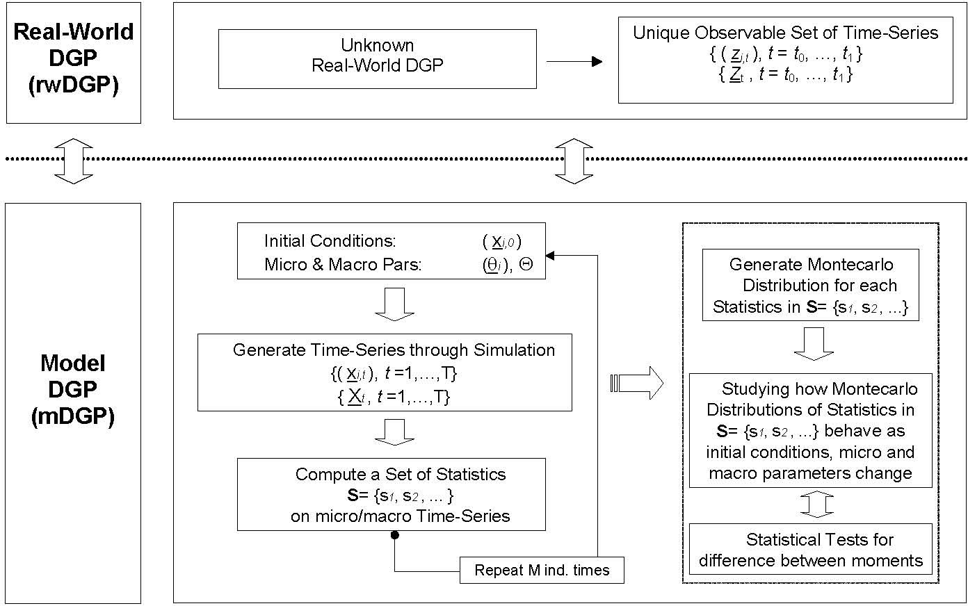
Figure 1. A procedure for studying the output of an AB model

3.3

The first dimension is the nature of the object(s) under study (first column of Table 1). These are the stylised facts (empirically observed facts) that the model is seeking to explain. Significant differences exist with respect to the nature of the object being studied in AB models. Examples range from qualitative change in economic systems due to R&D spending, through to quantitative objects such as statistically observed quantitative properties of aggregate growth, like autocorrelation patterns. Another important distinction exists between AB models that seek to investigate a single phenomenon such as aggregate growth, and those that jointly investigate multiple phenomena, such as aggregate growth together with productivity and investment patterns. The latter properties may in turn concern the transient or the long-run. Finally, AB models might investigate micro distributions (e.g. firm size) or macro aggregates (e.g., time-series properties of nation states, or the world economy).

3.4

A second dimension in which AB models differ is in the goal of the analysis (the second column of Table 1). AB models tend to deal with in-sample data (i.e., their prime aim is to replicate statistical properties of past data). Out-of-sample exercises (e.g., with the goal of answering control-related issues; making predictions; or addressing policy implications) are less frequently carried out by AB economists^[12].

3.5

A third dimension concerns the nature of the most important modelling assumptions (the third column of Table 1^[13]). Some models contain many degrees of freedom, others do not. For example, agents' decision rules in AB models may be characterised by many variables and parameters. Alternatively, they may be described in a very stylised way. Similarly, interaction structures may be exogenously fixed or they may change over time, either exogenously or endogenously (see e.g. Fagiolo et al. 2004b).

3.6

The fourth and final dimension is the method of sensitivity analysis (the fourth column of Table 1). In order to thoroughly assess the properties of an AB model, the researcher needs to perform a detailed sensitivity analysis along the lines sketched in Figure 1. This sensitivity analysis should, at the very least, explore how the results depend on (i) micro-macro parameters, (ii) initial conditions, and (iii) across-run variability induced by stochastic elements (e.g., random individual decision rules). More generally, sensitivity analysis entails a careful investigation of how the outputs of a model vary when one alters its inputs (Law and Kelton 1991; Leombruni et al. 2006). Therefore, apart from sampling the space of parameters and initial conditions, researchers need to check the robustness of the results against changes in (i) the distribution of random variables generating noise in the system, (ii) timing and updating mechanisms, and (iii) level of aggregation of microeconomic variables.

3.7

These four key dimensions strongly inform the choice of empirical validation procedure that is used. The focus on qualitative or quantitative phenomena, on micro or macro phenomena, and on transients or long-run impacts, determine the type of data that is required for empirical validation, the statistical procedures to be followed, and the ability to generate empirically testable implications. Additionally, the extent to which sensitivity analysis is performed prior to empirical validation has important implications for the universality of the simulation results that are obtained. Whether the analysis is a descriptive (in-sample) exercise, or seeks to generate out-of-sample predictions, it necessitates different approaches to data collection and analysis. Out-of-sample analysis requires the researcher to calibrate parameters and initial conditions. As discussed, this should be governed by empirical evidence (where it is available).

Table 1. Taxonomy of dimensions of heterogeneity in AB models

Alternative Approaches to Empirical Validation in AB Models

4.1: In this section, we review three of the most influential approaches to empirical validation that have been developed in the AB literature. These are the indirect calibration approach, the Werker-Brenner approach, and the history-friendly approach^[14]. Each attempts to reduce the number of model parameters, and to reduce the space of possible 'worlds' that are explored. Yet each does this in a very different way. The history-friendly approach constrains parameters, interactions, and decision rules in the model in line with the specific, empirically-observable history of a particular industry. It can be interpreted as a calibration exercise with respect to unique historical traces. The other two approaches do not impose a preliminary set of restrictions on parameters but, rather, indirectly employ empirical evidence to identify sub-regions in the potential parameter space. Within these sub-regions, a model is expected to replicate some relevant statistical regularities or stylised facts.
4.2: Some AB economists, engaged in qualitative modelling, are critical of the suggestion that meaningful empirical validation is possible. They suggest there are inherent difficulties in trying to develop an empirically-based social science that is akin to the natural sciences. Socio-economic systems, it is argued, are inherently open-ended, interdependent and subject to structural change. How can one then hope to effectively isolate a specific 'sphere of reality', specify all relations between phenomena within that sphere and the external environment, and build a model describing all important phenomena observed within the sphere (together with all essential influences of the external environment)? In the face of such difficulties, some AB modellers do not believe it is possible to represent the social context as vectors of quantitative variables with stable dimensions (e.g. Valente 2005).
4.3: One possible reaction is to use the computer as an artificial laboratory in which basic, causal relationships can be tested in order to gain some knowledge on the underlying (much more intricate and convoluted) real-world causal structure. The danger of this strategy is that one ends up building auto-referential formalisations that have no link to reality (Edmonds and Moss 2005). Certainly there are those in other social science disciplines who have taken the step of accepting they are constructing and analysing synthetic artificial worlds which may or may not have a link with the world we observe (Doran 1997). Those taking this position open themselves to the proposition that a model should be judged by the criteria that are used in mathematics: i.e. precision, importance, soundness and generality. This is hardly the case with AB models! The majority of AB modellers do not go down this particular path. Instead, they employ methodological approaches that seek to deal with the difficult issues and problems discussed in sections 2 and 3.
The Indirect Calibration Approach
4.4: Drawing upon a combination of stylised facts and empirical datasets, a number of AB modellers have been developing a pragmatic four-step approach to empirical validation (cf. Dosi et al. 2006). As its name suggests, the indirect calibration approach first performs validation, and then indirectly calibrates the model by focusing on the parameters that are consistent with output validation. In the first step, the modeller identifies a set of stylised facts that (s)he is interested in reproducing and/or explaining with a model. Stylised facts typically concern the macro-level (e.g. the relationship between unemployment rates and GDP growth) but can also relate to cross-sectional regularities (e.g. the shape of the distributions on firm size). In the second step, along with the prescriptions of the empirical calibration procedure, the researcher builds the model in a way that keeps the microeconomic description as close as possible to empirical and experimental evidence about microeconomic behaviour and interactions. This step entails gathering all possible evidence about the underlying principles that inform real-world behaviours (e.g. of firms, consumers, and industries) so that the microeconomic level is modelled in a not-too-unrealistic fashion. In the third step, the empirical evidence on stylised facts is used to restrict the space of parameters, and the initial conditions if the model turns out to be non-ergodic.
4.5: To illustrate, suppose that a Beveridge curve is one of the statistical regularities being investigated. The model must be able to replicate a relationship in which unemployment rates decrease with vacancy rates in the labour market (cf. Fagiolo et al. 2004a). The researcher should further restrict the analysis to all (and only) parameter combinations under which the model does not reject that hypothesis (at some confidence level). This step is the most sensible because it involves a fine sampling of the parameter space. It is also computationally demanding and requires the use of Monte Carlo techniques. For any given point in the parameter space, one must generate a distribution for the statistics summarising the stylised facts of interest (e.g. the slope of the relationship between unemployment and vacancy rate), and test the null hypothesis that the empirically observed value can be generated by the model under that particular parameter combination (see Figure 1).
4.6: In the fourth and final step, the researcher should deepen his/her understanding of the causal mechanisms that underlie the stylised facts being studied and/or explore the emergence of fresh stylised facts (i.e. statistical regularities that are different to the stylised facts of interest) which the model can validate ex post. This might be done by further investigating the subspace of parameters that are resistant to the third step, i.e. those consistent with the stylised facts of interest. For example, one might study how the absolute value of the Monte Carlo average of the slope of the unemployment-vacancy rate relation varies with some macro-parameter that governs wage setting and/or union power in the model. This can shed light on the causal mechanism underlying the emergence of a Beveridge curve. Similarly, one can ask whether business cycle properties (e.g. average and volatility of growth rates) change with the slope of the Beveridge relation. If this is the case, a fresh implication generated by the model (under empirically plausible parameters) can be taken to the data, and further provide support for the AB model under scrutiny.
4.7: A stream of recent AB contributions in the fields of industry and market dynamics has been strongly rooted in this four-step empirical validation procedure. For example, Fagiolo and Dosi (2003) study an evolutionary growth model that is able to reproduce many stylised facts of output dynamics, such as I(1) patterns of GNP growth, growth-rates autocorrelation structure, absence of size-effects, etc., while explaining the emergence of self-sustaining growth as the solution of the trade-off between exploitation of existing resources and exploration of new ones. Similarly, Fagiolo et al. (2004a) present a model of labour and output market dynamics that is not only able to jointly reproduce the Beveridge curve, the Okun curve and the wage curve, but also relates average growth rates of the system to the institutional set-up of the labour market. It must be noticed that many other AB contributions share the main principles underlying the indirect calibration approach to validation (Windrum 2004; Pyka and Fagiolo 2005). However, as discussed in Leombruni (2002), failure to address steps three and four will dramatically weaken the power of this approach.
4.8: While appealing, the indirect calibration approach is open to two criticisms. First, no attempt is made to calibrate micro and macro parameters using their empirical counterparts^[15]. There are two reasons for this. On the one hand, the models address in-sample exercises. On the other hand, due to the difficulties of matching theoretical and empirical observations, one must be agnostic as to whether the details of a model (variables, parameters) can be compared with empirically-observable ones. Yet, in order for this indirect, weak, calibration procedure to be effective, the empirical phenomena of interest should not be very general. Otherwise, they might not necessarily represent a difficult test for the model. If this is the case, the model might pass the validation procedure without providing any effective explanation of the phenomena of interest (e.g. no restrictions on the parameter space would be made). This parallels the identification/under-determination problem (see section 2) and Brock's discussion of 'unconditional objects' (Brock 1999). Here the fundamental issue of discriminating between the 'descriptions' and 'explanations' of reality arises once more.
4.9: The second criticism concerns the interpretation of the points belonging to the sub-region of the parameter space (and initial conditions) that resists the 'exercise in plausibility' performed in the third step of the procedure. After a suitable sub-region of the parameter space (and initial conditions) has been singled out — according to the capability of the model to replicate the set of stylised facts of interests in that sub-region — how should one interpret all comparative exercises that aim at understanding what happens when one tunes the parameters within that sub-region? This is the problem of interpreting the different parameter configurations as counterfactuals. It will be considered in more detail in section 5.
The Werker-Brenner Approach to Empirical Calibration
4.10: Empirical calibration of AB models has been proposed by Werker and Brenner (2004), and applied in Brenner and Murmann (2003), and Brenner (2004). The Werker-Brenner approach is a three-step procedure for empirical calibration. The first two steps are consistent with all calibration exercises. The third step is novel. The main difference with the Indirect Calibration approach is that here one tries to pick empirical parameters directly to calibrate the model. Step 1 uses existing empirical knowledge to calibrate initial conditions and the ranges of model parameters. Werker and Brenner propose that wide ranges should be specified for parameters for which there is little or no reliable data. Step 2 involves empirical validation of the outputs for each of the model specifications derived from Step 1. Through empirical validation, the plausible set of dimensions within the initial dimension space is further reduced. Werker and Brenner suggest that Bayesian inference procedures can be an option to practically conduct this output validation. Each model specification is assigned a likelihood of being accepted, based on the percentage of 'theoretical realisations' that are compatible with each 'empirical realisation'. In this way, empirically observed realisations are used to further restrict the initial set of model specifications (parameter values) that are to be considered. The modeller only retains those parameter values (i.e. model specifications) that are associated to the highest likelihood by the current known facts (i.e. empirical realisations). Model specifications that conflict with currently known data are discounted. Step 3 involves a further round of calibration. This uses the surviving set of models and, where helpful, recourse to expert testimony from historians. This they call 'methodological abduction'. In effect, one is trying to identify an underlying structural model from the shared properties and characteristics of the surviving models. The authors argue that "these [shared] characteristics can be expected to hold also for the real systems (given the development of the model has not included any crucial and false premises)" (Werker and Brenner 2004, p.13).
4.11: As with all approaches, there are strengths and weaknesses to empirical calibration. The Werker-Brenner approach is attractive in a number of respects. First, it addresses head-on many of the issues of model evaluation: it offers a means of reducing the degree of freedom in models and it advocates testing procedures for sensitivity analysis on large numbers of simulations. It also avoids a number of the potential pitfalls associated with developing models based on single case study histories. Second, it appears to offer a powerful methodology for developing rigorous, empirically-grounded simulation models; models that explicitly take into account competing theories and assumptions.
4.12: Let us consider some important methodological and operational issues associated with calibration. These, we hasten add, are not specific to Werker-Brenner, but are generic to all calibration approaches. First, assessing fitness amongst a class of models does not automatically help us identify a true underlying model (this is another version of the problem of identification introduced in section 2). If the initial set of models does not fit well, in the sense that it does not represent the true underlying model, then any likelihood-based method of selecting or averaging models can produce bad results (see Schorfheide 2000).
4.13: Second, there is a strong tendency for calibration to influence the types of models we develop. Notably, empirically calibrated models encourage the modeller to focus on variables and parameters that are readily calibrated and for which data already exists (Chattoe 2002). Yet, there are many potentially important variables and parameters for which data does not currently exist. Some may not be amenable to quantitative measurement. For instance, agents' mental models are an important component in many AB economics models. Yet the mental models used by real world agents tend to be unobservable in practice. The calibration approach tends to induce the modeller either to abstract from the micro features of the economy, or to force calibration of those parameters using unreliable or inconsistent data. The approach also impacts on the types of model outputs that are considered. Again, there is a temptation to focus on outputs that are readily measured, and not to consider phenomena that cannot be measured or calibrated a priori. There is an inherent conservativeness here, a conservativeness which inhibits the search for new theories and new explanatory variables.
4.14: A third issue is the quality of the available empirical data. The most common reason for under-determination in economics is the bias and incompleteness the available datasets. It is not always possible to exclude a particular model on the basis of existing empirical data because other types of data can potentially support the model, if they had been collected. Effective calibration requires a wealth of high quality data. Indeed, the Werker-Brenner calibration approach is particularly demanding because it requires the modeller to engage in two rounds of empirical validation. Unfortunately, in economics (and in the other social sciences, for that matter) empirical data is always scarce while the capacity of economists to generate new theories is potentially infinite (Friedman 1953).
4.15: A fourth issue highlighted by calibration is the nature of the relationship between the model mDGP and the real-world rwDGP. First, there is the question of whether the rwDGP is ergodic or non-ergodic. If the underlying real-world rwDGP is thought to be non-ergodic (as well as the theoretical mDGP described in the AB model), then initial conditions matter. This raises a whole host of problems for the modeller. The modeller needs to identify the 'true' set of initial conditions in the empirical data, generated by the rwDGP, in order to correctly set the initial parameters of the model. Even if perfect data exists (which is unlikely), this is a very difficult task. How far in the past does one need to go in order to identify the correct set of initial values for the relevant micro and macro variables? There is a possibility of infinite regress. If this is the case, then one may need data stretching back a very long time, possibly before data started to be collected.
4.16: Fifth, even when the mDGP and rwDGP are thought to be (sufficiently) stationary processes, the problem of correctly setting t₀ remains. An important decision to make is about the particular sub-sample of simulated data (of length τ = t_n - t₀) that is to be compared with the empirical data. The underlying rwDGP may generate a number of different regimes, e.g. the same macroeconomic structure may generate a diverse set of outcomes that include economic depression, full employment, inflation, hyper-inflation, and even stagflation. If this is the case, then one is faced with the problem of which sub-sample of simulated and observed time-series should be compared in order to carry out model validation. By incorrectly setting time t₀ in the model, one can generate a set of simulated output data that describes a different regime to that found in the empirical data. In addition to the issue of correctly setting t₀, one must identify the appropriate point at which to stop the simulation runs, i.e. to correctly set t_n. If t_n is set incorrectly then the simulated data may include multiple regimes that are covered by the empirical data. If the start or end points (or both) for the simulation runs are incorrectly set, there is the danger that one incorrectly rejects a 'true' model on the basis of its simulated outputs. We should also note that if, as is frequently the case, the modeller sets the simulation runs to end at a point where the model reaches a stationary or almost stationary behaviour, one is implicitly assuming that the empirical evidence comes from a stationary DGP. This may, or may not, be the case^[16].
4.17: What if the observed micro and macro parameters are time dependent? One needs to be sure that the empirically estimated parameters that we assume are slow changing variables (and, hence, can reasonably be treated as fixed within the timescale explored by the model) are not actually time dependent. If they are, then the researcher needs to go back and rethink the structural relationships between slow and fast variables, the timescale of the model^[17], or both.
The History-Friendly Approach
4.18: The history-friendly approach offers an alternative solution to the problem of over-parameterisation. Like the calibration approaches discussed above, it seeks to bring the model more closely in line with the empirical evidence. Thus, in comparisons with the other approaches, it emphasizes even more concretisation in the trade-off with isolation (see section 2). The key difference is that this approach uses the specific historical case studies of an industry to model parameters, agent interactions, and agent decision rules. In effect, it is a calibration approach which uses particular historical traces in order to calibrate a model.
4.19: In part, the history-friendly approach represents an attempt to deal with criticisms levelled at early neo-Schumpeterian AB models of technological change. Two of the key protagonists of history-friendly modelling, Richard Nelson and Sydney Winter, were founding fathers of neo-Schumpeterian AB modelling. While the early models were much more micro-founded and empirically-driven than contemporary neoclassical models, empirical validation was weak. There was a lack of thorough sensitivity and validation checks. Empirical validation, when carried out, tended to consist of little more than a cursory comparison of outputs generated by a handful of simulation runs with some very general stylised facts. Further, the early models contained many dimensions and so it was rather easy to generate a few outputs that matched some very general observations (the over-parameterisation problem)^[18].
4.20: In terms of our taxonomy, the history-friendly approach is strongly quantitative and mainly focuses on microeconomic transients (industrial paths of development). In this approach a 'good' model is one that can generate multiple stylised facts observed in an industry. The approach has been developed in a series of papers. Key amongst these is Malerba et al. (1999), and Malerba and Orsenigo (2001). In the first of these papers, the authors outlined the approach and then applied it to a discussion of the transition in the computer industry from mainframes to desktop PCs. In the second of these papers, the approach was applied to the pharmaceutical industry and the role of biotech firms therein. Here we shall keep the description of the approach succinct^[19]. Through the construction of industry-based AB models, detailed empirical data on an industry informs the AB researcher in model building, analysis and validation. Models are to be built upon a range of available data, from detailed empirical studies to anecdotal evidence to histories written about the industry under study. This range of data is used to assist model building and validation. It should guide the specification of agents (their behaviour, decision rules, and interactions), and the environment in which they operate. The data should also assist the identification of initial conditions and parameters on key variables likely to generate the observed history. Finally, the data is to be used to empirically validate the model by comparing its output (the 'simulated trace history') with the 'actual' history of the industry. It is the latter that truly distinguishes the history-friendly approach from other approaches. Previous researchers have used historical case studies to guide the specification of agents and environment, and to identify possible key parameters. The authors of the history-friendly approach suggest that, through a process of backward induction one can arrive at the correct set of structural assumptions, parameter settings, and initial conditions. Having identified the correct set of 'history-replicating parameters', one can carry on and conduct sensitivity analysis to establish whether (in the authors' words) 'history divergent' results are possible.
4.21: There are many points here that deserve closer inspection. Let us begin with issues that concern the structure of the model and the object of analysis. First, the modelling activity that has been conducted is, in practice, informed by the history of a few, key companies rather than the history of an entire industry. For instance, Malerba et al. (1999) is calibrated to capture one particular computer company — IBM — rather than the entire industry. This severely restricts the universality of the model. As a consequence, the micro-economic description of the supply-side of the industry is highly stylised. The demand-side of the computer industry model is also highly stylised. Indeed, many of the behavioural assumptions made about the supply and demand sides do not appear to be driven by industry-specific empirical observations. Windrum (2004) suggests that this reflects practical difficulties in collecting sufficient amounts of high quality data at the industry level.
4.22: This leads us to an important question: to what extent can one hope to acquire all the relevant data needed to build an empirically sound industry-level model? If this is not possible, then a further question follows: what are we to do if the empirical evidence is incomplete, offers no guidance on a particular point, or else seems to contain alternative, competing viewpoints?
4.23: Finally, limited attention is given to sensitivity analysis in the history friendly models, as parameters and rules are supposed to be deduced from the industry under study. The lack of sensitivity analysis is particularly noticeable with regards to cross-run variability.
4.24: Aside from the issues relating to implementation, the history-friendly approach raises a set of fundamental methodological issues. First, the approach to empirical validation that is advocated involves comparing the output traces of a simulated model with detailed empirical studies of the actual trace history of an economic system. We are immediately confronted, once again, with problems associated with comparing individual output traces generated by the model mDGP with individual traces generated by the real-world rwDGP. This does not move us much further on from ascertaining whether a model is 'capable' of generating an output trace that resembles an empirically observed trace. It is not a very strong test. An individual simulated trace may, or may not, be typical of the model. A second issue is the ability to backwardly induce the 'correct' set of structural assumptions, parameter settings, or initial conditions from a set of traces — even if we have a model that generates an appropriate distribution of output traces. Simply stated, there are, in principle, a great many combinations of alternative parameter settings that can produce an identical output trace. We cannot deduce which combination of parameter settings is correct, let alone the appropriate set of structural assumptions. A third issue concerns the possibility of constructing counterfactual histories (although the authors do not themselves engage in this in their papers). For example, we need to be able to construct a world in which IBM did not enter the PC market. This poses a very serious question. Could the PC market have developed in much the same way had IBM not invented the PC? Can we meaningfully construct a counterfactual history? As Cowan and Foray (2002) discuss, it is exceedingly difficult in practice to construct counterfactual histories because economic systems are stochastic, non-ergodic, and structurally evolve over time.
4.25: Finally, a fourth key methodological issue concerns the meaning of history: to what extent can we actually rely on history to be the final arbiter of theoretical and modelling debates? History itself is neither simple nor uncontested, and any attempt to develop a historically based approach to modelling faces deep-level methodological problems^[20]. The development of high quality accounts, open to critical scrutiny, is essential to the history-friendly approach. It is, after all, on the basis of these accounts that guidance is taken on particular modelling choices, on parameter testing, and output evaluation. In recognising the limitations of any historical account, we simultaneously identify the limitations of decisions based on that account. While a single 'typical' history may not exist, we may be able to draw some generalisations on the basis of a large collection of historical case studies. To use an analogy used by Jerry Silverberg, rather than seeking to develop a model that describes the fall of one particular leaf from a tree (the history friendly approach), we should seek to develop general models, such as the bromide diffusion model in physics, that can be used to explain the fall of many leaves from many trees (and other phenomena). To get to this point, what is needed is the construction of high quality datasets (see next section).

Future research issues

5.1

By applying the taxonomy developed in section 3, we can identify important differences between the three approaches with respect to the types of empirical data that are used and how these are applied in the process of empirical validation (see Table 2). First, there is the empirical domain addressed by each approach. The direct and indirect calibration approaches can, in principle, be applied to micro and macro AB models (e.g. to describe the dynamics of firms, industries, and countries). By contrast, the history-friendly approach only addresses micro dynamics. Second, there are differences between the types of empirical observations (data) used for empirical validation. In addition to empirical datasets, the Brenner-Werker approach advocates the use of historical knowledge. The history-friendly approach allows one to employ casual and anecdotal (based on particular experience or case studies) knowledge as well. Third, there are differences in the way data is actually used. All three approaches use data to assist model building, as well as validation of the simulated outputs of models. Unlike the other two approaches, indirect calibration does not directly employ data to calibrate initial conditions and parameters. Fourth, there are differences in the order in which validation and calibration is performed. Both the Werker-Brenner and the history-friendly approaches first perform calibration and then validation. By contrast, the indirect calibration approach first performs validation, and then indirectly calibrates the model by focusing on the parameters that are consistent with output validation.


Table 2: Differences between the types of data collected and their application

	Empirical domain	The types of data used	The application of data	Order of application
Indirect Calibration Approach	- Micro (industries, markets) - Macro (countries, world economy)	- Empirical data	- Assisting in model building - Validating simulated output	- First validate, then indirectly calibrate
Werker-Brenner Approach	- Micro (industries, markets) - Macro (countries, world economy)	- Empirical data - Historical knowledge	- Assisting in model building - Calibrating initial conditions and parameters - Validating simulated output	- First calibrate, then validate
History-Friendly Approach	- Micro (industries, markets)	- Empirical data - Casual, historical and anecdotic knowledge	- Assisting in model building - Calibrating initial conditions and parameters - Validating simulated output	- First calibrate, then validate

5.2

The foregoing discussion has highlighted a set of core issues that affect all the approaches and which (so far) remain unresolved. In this section we shed some light on those issues.

Alternative strategies for constructing empirically-based models. There is intense debate about the best way to actually construct empirically-based models, and to select between alternative models. What happens, for instance, if there are alternative assumptions and existing empirical data does not assist in choosing between them? A number of different strategies exist for selecting assumptions in the early stages of model building (Edmonds and Moss 2005). One strategy is to start with the simplest possible model, and then proceed to complicate the model step-by-step. This is the KISS strategy: "Keep it simple, stupid!" A very different strategy is the KIDS strategy: "Keep it descriptive, stupid!" Here one begins with the most descriptive model one can imagine, and then simplifies it as much as possible. The third strategy, common amongst neoclassical economists, is TAPAS: "Take A Previous model and Add Something" (Frenken 2005). Here one takes an existing model and successively explores the assumption space through incremental additions and/or the relaxation of initial assumptions.
Problems that arise as a consequence of over-parameterisation in AB models. Whatever the strategy employed, the AB modeller often faces an over-parameterisation problem. AB models with realistic assumptions and agent descriptions invariably contain many degrees of freedom. There are two aspects to the over-parameterisation problem. Firstly, the dimensions of the model may be so numerous that it can generate any result. If this is the case, then the explanative potential of the model is little better than a random walk. Secondly, the causal relations between assumptions and results become increasingly difficult to study. A possible strategy is to use empirical evidence to restrict the degrees of freedom, by directly calibrating initial conditions and/or parameters (see section 4). Then, one can reduce the degrees of freedom of the model by focussing on the subspace of parameters and initial conditions under which the model is able to replicate a set of stylised facts (as in the indirect calibration approach discussed in 4.4). Unfortunately, this procedure often tends to leave the modeller with multiple possible 'worlds'.
The usefulness and implications of counterfactuals for policy analysis. How does one interpret the counterfactual outputs generated by a model? It is tempting to suggest that outputs which do not accord with empirical observations are counterfactuals, and that the study of these counterfactuals is useful for policy analysis. Cowan and Foray (2002) suggest that it is exceedingly difficult, in practice, to construct counterfactual histories because economic systems are stochastic, non-ergodic, and structurally evolve over time. As AB models typically include all these elements in their structure, Cowan and Foray argue that using (evolutionary) AB models to address counterfactual-like questions may be misleading. More generally, comparing the outputs generated by AB models with real-world observations involves a set of very intricate issues. For example, Windrum (2004) observes that the uniqueness of historical events sets up a whole series of problems. In order to move beyond the study of individual traces, we need to know if the distribution of output traces generated by the model mDGP approximates the actual historical traces generated by the rwDGP under investigation. A way to circumvent the uniqueness problem is to employ a strong invariance assumption on the rwDGP, thereby pooling data that should otherwise be considered a set of unique observations. For example, one typically supposes that cross-country aggregate output growth rates come from the same DGP. Similarly, it is supposed that the process that driving firm growth does not change across industries or time (up to some mean or variance scaling). This allows one to build cross-section and time-series panel data. Unfortunately we cannot know if these suppositions are valid. But this is often not possible in practice. Consider the following example. Suppose the rwDGP in a particular industry does not change over time (i.e. it is ergodic). Even if this is the case, we do not typically observe the entire distribution of all observations but rather a very limited set of observations — possibly only one, unique roll of the dice. The actual history of the industry we observe is only one of a set of possible worlds. So how do we know that the actual historical trace is in any sense typical (statistically speaking) of the potential distribution? If we do not know this, then we have nothing against which to compare the distributions generated by our model. We cannot determine what is typical, and what is atypical.^[21]
Definition of sufficiently strong empirical tests. The fundamental difficulties in defining strong tests for model outputs is highlighted by Brock's (1999) discussion of "unconditional objects" in economics. Empirical regularities need to be handled with care because we only have information on the properties of stationary distributions. The data that we observe does not provide information on the dynamics of the stochastic processes that actually generated them. Therefore, replication does not necessary imply explanation. For example, many evolutionary growth models can generate similar outputs on differential growth-rates between countries, technology leadership and catch-up, even though they differ significantly with respect to the behaviour and learning procedures of agents, and in their causal mechanisms (Windrum 2004). Similarly, the Nelson and Winter (1982) model replicates highly aggregated data on time paths for output (GDP), capital and labour inputs, and wages (labour share in output), but these outputs can also be replicated by conventional neoclassical growth models. In the same vein, there might be many different stochastic processes (and therefore industry dynamic models) that are able to generate, as a stationary state, a power-law distribution for the cross-section firm size distribution. Although one may be unable to narrow down a single model, we may be able to learn about the general forces at work, and to restrict the number of models that can generate a set of statistical regularities (Brock 1999). Therefore, so long as the set of stylised facts to be jointly replicated is sufficiently large, any `indirect' validation could be sufficiently informative, because it can effectively help in restricting the set of all stochastic processes that could have generated the data displaying those stylised facts. Another way out of the conditional objects critique would be to not only validate the macro-economic output of the model, but also its micro-economics structure, e.g. agents' behavioural rules. This requires one to only include in the model individual decision rules (e.g. learning) that have been validated by empirical evidence. Of course, this would require highly detailed and reliable data about microeconomic variables, possibly derived from extensive laboratory experiments.
Availability, quality and bias of datasets. Empirically-based modelling depends on high quality datasets. Unfortunately, the datasets that exist are invariably pre-selected. Not all potential records are retained; some are fortuitously bequeathed by the past but others are not captured. Datasets are constructed according to criteria that reflect certain choices and, as a consequence, are biased. As econometricians know only too well, it may simply be the case that data which would have assisted in a particular discussion has simply not been collected. A further and often neglected problem is that standard econometric methods are influenced by prevailing theoretical orthodoxy.

Conclusions

6.1: This paper has critically examined a set of core issues for the empirical validation of AB simulation models. Sections 1 and 2 defined what an AB model is, and the methodological basis of empirical validation. Six core issues associated with empirical validation were identified. There is no consensus on how these issues have to be tackled. Indeed, a set of different approaches is being developed by AB economists. This was addressed in the remainder of the paper. In section 3 we presented a novel taxonomy which contains four significant dimensions along which the various approaches differ. Having identified the nature and causes of heterogeneity amongst AB modellers, section 4 narrowed the focus by discussing three important approaches to validation within AB economics: indirect calibration, the Werker-Brenner calibration approach, and the history-friendly approach. The taxonomy was applied to the three approaches and enabled us to identify key differences between the types of empirical data used by these approaches and in their application of data. We were also able to examine how, in different ways, each approach deals with the six generic issues of empirical validation. In section 5 we have identified a set of unresolved problems that require future research.
6.2: To conclude, the AB economics community has been extremely successful in developing models that address issues that were not amenable using traditional neoclassical models (Dosi et al. 1994). These AB models are able to explain how some crucial macroeconomic phenomena can be generated by the evolving networks of interactions among boundedly-rational agents in economies where the fundamentals may endogenously evolve over time. Examples range from growth and development patterns, to industry and market dynamics, to technological innovation, to the evolution of consumption and demand. What is more, they did so by taking on board methodological pluralism and avoiding the apriorist view that characterises neoclassical economics. Having said this, there are a set of core issues that need to be addressed by the AB economics community if it is to proceed successfully. Notably, there is an excess of heterogeneity with respect to the range of competing models and a lack of consensus on core methodological questions. Drawing upon the findings of this paper, we suggest two fruitful directions. First, a commonly accepted, minimal protocol for the analysis of AB models should be developed and agreed upon (here we concur with Leombruni (2002) and Leombruni et al. (2006)). This would allow AB models to become more comparable and reach more methodologically sound conclusions. Second, far more work needs to be done to address the 6 core issues of empirical validation discussed in the paper. We believe that the recent trend, which seems to indicate a growing interest in methodological questions within the AB community, is an optimistic move in this direction.

Notes

¹We do not aim to provide a complete survey of AB models in economics, nor to discuss the (often subtle) differences that characterise the different research schools that have been using AB models to study market and industry dynamics (e.g. evolutionary economics, agent-based computational economics, neo-Schumpeterian, and history-friendly models). The interested reader is referred to Lane (1993a, 1993b), Dosi and Nelson (1994), Nelson (1995), Silverberg and Verspagen (1995), Tesfatsion (1997, 2002), Windrum (2004), Dawid (2006), and Pyka and Fagiolo (2005). Also see Gilbert and Troitzsch (1999), and Wooldridge and Jennings (1995) for a discussion of AB techniques in other social sciences.

²An alternative view (though one which we doubt would be shared by most AB economists themselves) is that the AB approach is complementary to neoclassical economics. Departures from standard neoclassical assumptions, found in AB models, can be interpreted as 'what if', instrumentalist explorations of the space of initial assumptions. For example, what happens if we do not suppose hyper-rationality on the part of individuals?, What if agents decide on the basis of bounded rationality?

³At a special session on 'Methodological Issues in Empirically-based Simulation Modelling', hosted by Fagiolo and Windrum at the 4th EMAEE conference, Utrecht, May 2005, and at the ACEPOL 2005 International Workshop on 'Agent-Based Models for Economic Policy Design', Bielefeld, July 2005.

⁴Quite often it is not only impossible not only to know the real world DGP but also to get good a quality data set on the 'real world'. The latter problem is discussed in section 5.

⁵The focus in this paper is the concept of empirical validity. That is, the validity of a model with respect to data. There are other meanings of validity, which are in part interrelated with empirical validity, but which we will not consider here. Examples include model validity (the validity of a model with respect to the theory) and program validity (the validity of the simulation program with respect to the model). The reader is referred to Leombruni et al. (2006).

⁶Indeed, several possible qualifications of realism are possible (see Mäki 1998).

⁷The reader is referred to Moneta (2005) for an account of realist and anti-realist positions on causality in econometrics.

⁸The main theories of confirmation can be divided in probabilistic theories of confirmation, in which evidence in favour of a hypothesis is evidence that increases its probability, and non-probabilistic theories of confirmation, associated with Popper, Fisher, Neyman and Pearson. The reader is referred to Howson (2000).

⁹For example, one of the micro variables might be an individual firm's output and the corresponding macro variable may be GNP. In this case, we may be interested in the aggregate statistic s_j defined as the average rate of growth of the economy over T time-steps (e.g. quarterly years).

¹⁰Consider the example of the previous footnote once again. One may plot E(s_j), that is the Monte-Carlo mean of aggregate average growth rates, against key macro parameters such as the aggregate propensity to invest in R&D. This may allow one to understand whether the overall performance of the economy increases in the model with that propensity. Moreover, non-parametric statistical tests can be conducted to see if E(s_j) differs significantly in two extreme cases, such as a high vs. low propensity to invest in R&D.

¹¹Space constraints prevent us from discussing how different classes of AB models (e.g. evolutionary industry and growth models, history-friendly models, and ACE models) fit each single field of the entries in Table 1. See Windrum (2004), and Dawid (2006) for detailed discussions of this topic. The taxonomy presented in Table 1 partly draws from Leombruni et al. (2006). The reader is also referred to Leigh Tesfatsion's web site on empirical validation (http://www.econ.iastate.edu/tesfatsi/empvalid.htm).

¹²For examples along this line, see Marks 2005; Koesrindartoto et al., 2005; and the papers presented at the recent conference 'Agent-Based Models for Economic Policy Design' (ACEPOL05), Bielefeld, June 30, 2005 - July, 2, 2005 (http://www.wiwi.uni-bielefeld.de/~dawid/acepol/).

¹³The pros and cons of this heterogeneity in modelling assumptions for AB economists were discussed in section 1 of this paper. Also see Richiardi (2003), Pyka and Fagiolo (2005), and Leombruni et al. (2006).

¹⁴In discussing these three approaches we do not claim exhaustiveness (indeed other methods can be conceived). We selected these approaches because they are the most commonly used approaches to validate AB economics models.

¹⁵Obviously, there is no methodological prohibition of doing that. However, the researcher often wants to keep as much degrees of freedom as possible.

¹⁶See for example the calibration exercises performed by Bianchi et al. (2005) on the CATS model developed in a series of papers by Gallegati et al. (2003, 2005).

¹⁷An important issue related to time-scales in AB models, which we shall just mention here, concerns the choice made about timing in the model. Whether we assume that the time-interval [t, t+1] describes a day, or a quarter, or a year (and whether one supposes that the 'updating scheme' is asynchronous or parallel), has non-trivial consequences for calibration and empirical validation.

¹⁸See Windrum (1999) for a detailed discussion of early neo-Schumpeterian models.

¹⁹Interested readers are directed to Windrum (2004) for a detailed critique of history-friendly modelling.

²⁰A well-known example of the contestability of history is evidenced by the ongoing debate about whether inferior quality variants can win standards battles (Leibowitz and Margolis 1990; Arthur 1988). As Carr (1961) observed in his classic work, history can be contestable at more fundamental and unavoidable levels.

²¹A quite related open-issue, as suggested by an anonymous referee, is the inter-relationship between validation and policy implications. Indeed, if one is concerned with a particular policy question, one could have a more pragmatic approach of the kind: "validation of the model for the purpose at hand is successful if, using the available observations of the rwDGP, the set of potential mDGPs can be restricted in a way that the answer to the posed policy question is the same no matter which mDGP from that set is chosen".

References

ARTHUR W B (1988) Competing technologies: an overview. In Dosi G, Freeman C, Nelson R, Silverberg G and Soete L (Eds.) Technical Change and Economic Theory. London: Pinter. pp. 590-607.

BIANCHI C, Cirillo P, Gallegati M and Vagliasindi P (2005) Validation in ACE models. An investigation of the CATS model. Unpublished Manuscript.

BRENNER T (2004) Agent learning representation — advice in modelling economic learning, Papers on Economics and Evolution. Jena: Max Planck Institute.

BRENNER T and Murmann, J P (2003) The use of simulations in developing robust knowledge about causal processes: methodological considerations and an application to industrial evolution, Papers on Economics and Evolution #0303. Jena: Max Planck Institute.

BROCK W (1999) Scaling in economics: a reader's guide. Industrial and Corporate Change, 8, pp. 409-446.

CARR E H (1961) What is History?, London: Macmillan.

CHATTOE E (2002) Building Empirically Plausible Multi-Agent Systems: A Case Study of Innovation Diffusion. In Dautenhahn K (Ed.) Socially Intelligent Agents: Creating Relationships with Computers and Robots. Dordrecht Kluwer.

COWAN R and Foray D (2002) Evolutionary economics and the counterfactual threat: on the nature and role of counterfactual history as an empirical tool in economics, Journal of Evolutionary Economics, 12 (5), pp. 539-562.

DAWID H (2006) Agent-based models of innovation and technological change. In Tesfatsion L and Judd K (Eds.) Handbook of Computational Economics II: Agent-based Computational Economics, Amsterdam: North-Holland.

DORAN J (1997) From computer simulation to artificial societies. SCS Transactions on Computer Simulation, 14 (2), pp. 69-78.

DOSI G (1988) Sources, procedures and microeconomic effects of innovation. Journal of Economic Literature, 26, pp. 126-171.

DOSI G., Fagiolo G. and Roventini A. (2006) An Evolutionary Model of Endogenous Business Cycles. Computational Economics, 27, pp. 3-34.

DOSI G, Freeman C and Fabiani S (1994) The process of economic development: introducing some stylized facts and theories on technologies, firms and institutions. Industrial and Corporate Change, 3, pp. 1-46.

DOSI G and Nelson R R (1994) An introduction to evolutionary theories in economics. Journal of Evolutionary Economics, 4, pp. 153-172.

DOSI G and Orsenigo L (1994) Macrodynamics and microfoundations: an evolutionary perspective. In Granstrand O (Ed.) The economics of technology. Amsterdam: North Holland.

DOSI G, Marengo L and Fagiolo G (2005) Learning in Evolutionary Environment. In Dopfer K (Ed.) Evolutionary Principles of Economics. Cambridge: Cambridge University Press.

EDMONDS B and Moss S (2005) From KISS to KIDS — an 'anti-simplistic' modelling approach. In Davidsson P, Logan B, Takadama K (Eds.) Multi Agent Based Simulation 2004. Lecture Notes in Artificial Intelligence. Springer, 3415, pp.130-144.

FAGIOLO G (1998) Spatial interactions in dynamic decentralized economies: a review. In Cohendet P, Llerena P, Stahn H and Umbhauer G (Eds.) The Economics of Networks. Interaction and Behaviours, Berlin — Heidelberg: Springer Verlag.

FAGIOLO G and Dosi G (2003) Exploitation, Exploration and Innovation in a Model of Endogenous Growth with Locally Interacting Agents, Structural Change and Economic Dynamics, 14, pp. 237-273.

FAGIOLO G, Dosi G and Gabriele R (2004a) Matching, Bargaining, and Wage Setting in an Evolutionary Model of Labor Market and Output Dynamics, Advances in Complex Systems, 14, pp. 237-273.

FAGIOLO G, Marengo L and Valente M (2004b) Endogenous Networks in Random Population Games. Mathematical Population Studies, 11, pp. 121-147.

FRENKEN K. (2005) History, state and prospects of evolutionary models of technical change: a review with special emphasis on complexity theory, Utrecht University, The Netherlands, mimeo.

FRIEDMAN M (1953) The Methodology of Positive Economics, in Essays in Positive Economics. Chicago: University of Chicago Press.

GALLEGATI M, Giulioni G, Palestrini A and DelliGatti D (2003) Financial fragility, patterns of firms' entry and exit and aggregate dynamics. Journal of Economic Behavior and Organization, 51, pp. 79-97.

GALLEGATI M, Gatti D D, Guilmi C D, Gaeo E, Giulioni G and Palestrini A (2005) A new approach to business fluctuations: heterogeneous interacting agents, scaling laws and financial fragility. Journal of Economic Behavior Organization, 56, pp. 489-512.

GIBBARD A and Varian H (1978) Economic Models. Journal of Philosophy, 75, pp. 664-677.

GILBERT N and Troitzsch K (1999) Simulation for the Social Scientist. Milton Keynes: Open University Press.

HAAVELMO T (1944) The Probability Approach in Econometrics, Econometrica, 12, pp. 1-115.

HOWSON C (2000) Evidence and Confirmation. In Newton-Smith W H (Ed.) A Companion to the Philosophy of Science. Malden, MA: Blackwell Publishers, pp. 108-116.

JANSSEN M C W (1994) Economic Models and Their Applications, Poznan Studies in the Philosophy of the Science and the Humanities, 38, pp. 101-116.

KIRMAN A P (1997a) The Economy as an Interactive System. In Arthur W B, Durlauf S N and Lane D (Eds.) The Economy as an Evolving Complex System II, Santa Fe Institute, Santa Fe and Reading, MA: Addison-Wesley.

KIRMAN A P (1997b) The Economy as an Evolving Network, Journal of Evolutionary Economics, 7, pp. 339-353.

KNIGHT F H (1921) Risk, Uncertainty, and Profits. Chicago: Chicago University Press.

KOESRINDARTOTO D, Sun J and Tesfatsion L (2005) An Agent-Based Computational Laboratory for Testing the Economic Reliability of Wholesale Power Market Designs, IEEE Power Engineering Society Conference Proceedings.

LAKATOS I (1970) Falsification and the Methodology of Scientific Research Programmes. In Lakatos I and Musgrave A, Criticism and the Growth of Knowledge, Cambridge: Cambridge University Press, pp. 91-196.

LANE D (1993a) Artificial worlds and economics, part I, Journal of Evolutionary Economics, 3, pp. 89-107.

LANE D (1993b) Artificial worlds and economics, part II, Journal of Evolutionary Economics, 3, pp. 177-197.

LAW A and Kelton W D (1991) Simulation Modeling and Analysis. New York: McGraw-Hill.

LEAMER E E (1978) Specification Searches, Ad Hoc Inference with Nonexperimental Data. New York: John Wiley.

LIEBOWITZ S J and Margolis S E (1990) The Fable of the Keys, Journal of Law and Economics, 22, pp. 1-26.

LEOMBRUNI R (2002) The Methodological Status of Agent-Based Simulations, Working Paper No. 19. Turin, Italy: LABORatorio R. Revelli, Centre for Employment Studies.

LEOMBRUNI R, Richiardi M, Saam, N and Sonnessa M. (2006) A Common Protocol for Agent-Based Social Simulation, Journal of Artificial Societies and Social Simulation, 9(1) https://www.jasss.org/9/1/15.html.

MÄKI U (1992) On the Method of Isolation in Economics, Poznan Studies in the Philosophy of the Sciences and the Humanities, 26, pp. 19-54.

MÄKI U (1998) Realism. In Davis J B, Hands D W and Mäki U (Eds.) The Handbook of Economic Methodology. Cheltenham, UK: Edward Elgar. pp. 404-409.

MÄKI U (2003) 'The methodology of positive economics' (1953) does not give us the methodology of positive economics, Journal of Economic Methodology, 10(4), pp. 495-505.

MÄKI U (2005) Models are experiments, experiments are models, Journal of Economic Methodology, 12(2), pp. 303-315.

MALERBA F and Orsenigo L (2001) Innovation and market structure in the dynamics of the pharmaceutical industry and biotechnology: towards a history friendly model, Conference in Honour of Richard Nelson and Sydney Winter, Aalborg, 12th — 15th June 2001.

MALERBA F, Nelson R R, Orsenigo L and Winter S G (1999) History friendly models of industry evolution: the computer industry, Industrial and Corporate Change, 8, pp. 3-41.

MARENGO L and Willinger M (1997) Alternative Methodologies for Modeling Evolutionary Dynamics: Introduction, Journal of Evolutionary Economics, 7, pp. 331-338

MARKS B (2005) Agent-Based Market Design, Australian Graduate School of Management, mimeo.

MONETA A (2005) Causality in Macroeconometrics: Some Considerations about Reductionism and Realism, Journal of Economic Methodology, 12(3), pp. 433-453.

MORRISON M and Morgan M S (1999) Models as mediating instruments. In Morgan M S and Morrison M (Eds.) Models as Mediators. Perspectives on Natural and Social Science. Cambridge: Cambridge University Press. pp. 10-37,

NELSON R R and Winter S G (1982) An Evolutionary Theory of Economic Change. Cambridge: Harvard University Press.

NELSON R R (1995) Recent Evolutionary Theorizing About Economic Change, Journal of Economic Literature, 33, pp. 48-90.

PYKA A and Fagiolo G (2005) Agent-Based Modelling: A Methodology for Neo-Schumpeterian Economics. In Hanusch H and Pyka A (Eds.) The Elgar Companion to Neo-Schumpeterian Economics. Cheltenham: Edward Elgar.

RICHIARDI M (2003) The Promises and Perils of Agent-Based Computational Economics, Working Paper No. 29. Turin, Italy: LABORatorio R. Revelli, Centre for Employment Studies.

SAVIOTTI P P and Pyka A (2004) Economic development, qualitative change and employment creation, Structural Change and Economics Dynamics, 15(3), pp. 265-287.

SAWYER K R, Beed C and Sankey H (1997) Underdetermination in Economics. The Duhem-Quine Thesis, Economics and Philosophy 13, pp. 1-23.

SCHORFHEIDE F (2000) Loss function-based evaluation of DSGE models, Journal of Applied Econometrics, 15(6), pp. 645-670.

SILVERBERG G and Verspagen B (1995) Evolutionary theorizing on economic growth, IIASA, Laxenburg, Austria, Working Paper, WP-95-78.

SILVERBERG G, Dosi G and Orsenigo L (1988) Innovation, diversity and diffusion: a self-organisation model, Economic Journal, 98, pp. 1032-1054.

TESFATSION L (1997) How Economists Can Get A Life. In Arthur, W, Durlauf S and Lane D (Eds.) The Economy as an Evolving Complex System II. SantaFeInstitute, Santa Fe and Reading, MA: Addison-Wesley.

TESFATSION L (2002) Agent-based Computational Economics: Growing Economies from the Bottom Up, Artifical Life, 8, pp. 55-82.

VALENTE M (2005) Qualitative Simulation Modelling, Faculty of Economics, University of L'Aquila, L'Aquila, Italy, mimeo.

WERKER C and Brenner T (2004) Empirical Calibration of Simulation Models, Papers on Economics and Evolution # 0410. Jena: Max Planck Institute for Research into Economic Systems.

WINDRUM P (1999) Simulation models of technological innovation: a review, American Behavioral Scientist, 42(10), pp. 1531-1550.

WINDRUM P (2004) Neo-Schumpeterian simulation models, Merit Research Memoranda 2004-004, MERIT, University of Maastricht. Forthcoming in Hanusch H and Pyka A (Eds.) The Elgar Companion to Neo-Schumpeterian Economics. Cheltenham: Edward Elgar.

WINDRUM P (2005) Heterogeneous preferences and new innovation cycles in mature industries: the camera industry 1955-1974, Industrial and Corporate Change, 14(6), pp. 1043-1074.

WINDRUM P and Birchenhall C (1998) Is life cycle theory a special case?: dominant designs and the emergence of market niches through co-evolutionary learning, Structural Change and Economic Dynamics, 9, pp. 109-134.

WOOLDRIDGE M and Jennings N R (1995) Intelligent agents: theory and practice, Knowledge Engineering Review, 10, pp. 115-152.

Button Return to Contents of this issue