©Copyright JASSS

JASSS logo ----

Noam Bergman, Alex Haxeltine, Lorraine Whitmarsh, Jonathan Köhler, Michel Schilperoord and Jan Rotmans (2008)

Modelling Socio-Technical Transition Patterns and Pathways

Journal of Artificial Societies and Social Simulation vol. 11, no. 3 7
<https://www.jasss.org/11/3/7.html>

For information about citing this article, click here

Received: 06-Jan-2008    Accepted: 13-May-2008    Published: 30-Jun-2008

PDF version


* Abstract

We report on research that is developing a simulation model for assessing systemic innovations, or 'transitions', of societal systems towards a more sustainable development. Our overall aim is to outline design principles for models that can offer new insights into tackling persistent problems in large-scale systems, such as the European road transport system or the regional management of water resources. The systemic nature of these problems is associated with them being complex, uncertain and cutting across a number of sectors, and indicates a need for radical technological and behavioural solutions that address changes at the systems level rather than offering incremental changes within sub-systems. Model design is inspired by recent research into transitions, an emerging paradigm which provides a framework for tackling persistent problems. We use concepts from the literature on transitions to develop a prototype of a generic 'transition model'. Our prototype aims to capture different types of transition pathways, using historical examples such as the transition from horse-drawn carriages to cars or that from sailing ships to steam ships. The model combines agent-based modelling techniques and system dynamics, and includes interactions of individual agents and sub-systems, as well as cumulative effects on system structures. We show success in simulating different historical transition pathways by adapting the model's parameters and rules for each example. Finally, we discuss the improvements necessary for systematically exploring and detailing transition pathways in empirical case-study applications to current and future transitions such as the transition to a sustainable transport system in Europe.

Keywords:
Complex Systems, Agent-Based Modelling, Social Simulation, Transitions, Transition Theory

* Introduction

1.1
We report on a modelling exercise conducted within the EU Framework Six MATISSE project[1], an EU Framework Six project developing prototypes of a new class of simulation model for assessing transitions towards sustainability. They are integrated models emphasising that societal systems are comprised of inter-locking sub-systems and that evolutionary societal change is a complex process. The models rely on the emerging field of transition science, which studies long-term societal and technical systemic changes, or transitions. We use concepts from the transitions literature (Geels 2005a; Rotmans et al. 2001) to develop a novel model of socio-technical transitions. While this literature includes analyses from historical examples (Geels 2002) and steering models (Loorbach and Rotmans 2006), simulation models of social transitions are still absent.

1.2
The overall context for this work is the development of tools for integrated sustainability assessment (ISA) and supporting ISA in EU policy-making (Turnpenny et al. 2007; Weaver 2005). This field is responsible for the portfolio of models and participatory methods that support the development of integrated sustainability policies. The particular research presented here aims to develop prototypes of a new generation of simulation modelling tools for use in ISAs. Simulations models are urgently needed for assessing potential transition pathways of societal systems towards a more sustainable development, and should aim to be relevant and useful to stakeholders and policymakers from the local to EU levels.

Transitions and modelling

1.3
Transitions research focuses on understanding radical, systemic socio-technical change. By 'radical' or 'systemic' change, we refer to system-exceeding change, i.e. a change that goes beyond the ordering of the current system. This typically occurs over decadal time scales. The literature on transitions has grown significantly over the past decade, pioneered by Kemp and Rip (1998), Geels (2002, 2005a, 2005b, 2006a, 2006b) and others (e.g., Rotmans 2005; Smith et al. 2005). Increasingly there is an interest in applying this understanding to addressing current problems of unsustainability by identifying how societal change towards more sustainable states may be fostered (e.g., Elzen et al. 2004; Hoogma et al. 2002). This transitions research in turn builds on the literature on technological innovation and industrial transformation (e.g., Diederen et al. 2003; Dosi 1984; Rogers 1995) and on theories of social change (e.g., Giddens 1984; Noble 2000). Crucially, this literature exposes the heterogeneity of populations (i.e., individuals and firms are differentiated by their innovativeness, resources and preferences) and the complex co-evolution of a range of actors and structures (e.g., firms, consumers, legislation, technologies and infrastructure) in processes of social change.

1.4
Our research aims to develop novel modelling tools which can simulate and assess transitions. Here, we introduce a general prototype model, which may be regarded as a first stage of this model development project. We then use four simplified historical examples in an attempt to reproduce a set of socio-technical transition pathways developed by Geels and Schot (2007). While Geels (2005a; 2005b; 2006a, 2006b) focuses on (socio-)technical transitions, which look at disruptive new technologies and the surrounding institutions, we are also interested in societal transitions (Rotmans et al. 2001), which encompass the broader picture of shifts in behaviour and societal functions as well as technologies. However, attempting to reproduce Geels' typology of socio-technical transitions provides an extremely useful test of the model. In parallel work the model is being applied with a more in-depth approach to a set of empirical case studies including a transition to sustainability mobility in Europe (Whitmarsh and Nykvist 2008; Köhler et al. forthcoming), a transition to sustainable housing in the UK (Bergman et al. 2007; Bergman et al. 2008), sustainable water management in Spain, and a more in-depth historical case study of the 19th century sail to steam transition in ocean shipping (Köhler and Schilperoord unpublished).

1.5
Eventually this research aims to generate modelling tools that can provide new insights into EU-wide problems, such as road transport or dematerialisation, which are persistent and intractable in nature. The systemic, complex and uncertain nature of these problems suggests a need for more radical technological and behavioural solutions to adequately address them. These are structural issues — deeply rooted in, and reinforced by, patterns of behaviour, technologies, infrastructures and social institutions (Geels 2005a). This highlights the need to address the underlying structural determinants of the problems, and ultimately encourage system-exceeding transformations to move beyond them. Therefore increasing attention is being given to radical, systemic innovation, or transitions as a means of tackling these types of persistent problems (Rotmans et al. 2001); and it is to this policy-relevant research agenda that the work presented here is responding.

1.6
The modelling approach presented here is not seen as leading to predictive models in any traditional sense of the word, but it is rather seen as being a heuristic device that is able to add value if used in a context of interaction with users, where it may be able to generate novel insights about the dynamics involved in entrenchment and lock-in on the one hand, and societal transitions on the other hand. We use historical examples as a means of model calibration and evaluation. However, our intention is not to recreate the full detail of the historical transition, but rather test how socio-economic and technical dynamics are captured in the model.

1.7
There are very few numerical models of transitions in the literature. While 'transition models' exist, they are mostly collapsed into economics, with shifts occurring as new technologies emerge (Köhler et al. 2006; Schwoon 2005). These models do not fully integrate social dynamics and environmental change with economic processes, and therefore do not simulate transitions in a way that is consistent with current theory or empirical evidence about transitions. There is a need for mechanisms, which may be market-driven, but are a complex mix of economic, political, social, cultural, and ecological mechanisms that cannot be collapsed into economics alone. It is this gap that we hope to begin to fill with this modelling exercise. In parallel work, we put together a conceptual framework (Haxeltine et al. 2008) for transition modelling. Section 2 of this paper introduces transition theory concepts central to our work, including a taxonomy of four transition pathways, which we use in this paper. Section 3 gives a detailed description of our model. Section 4 details our implementation of four stylised historical examples, one for each transition pathway, and Section 5 analyses the results. Finally, in Section 6 we summarise and draw conclusions from this work.

* Concepts in transition theory

Regimes, niches and regime change

2.1
Transition theory literature highlights the interdependency of institutions and infrastructures constituting societal systems and sub-systems, which has created various types of lock-in that stie innovation (Smith et al. 2005). These societal systems comprise inter-locking economic, social, cultural, infrastructural and regulative sub-systems, which are associated with a range of social groups (Geels 2005a). The stability and cohesion of societal systems is established and reinforced through cognitive, normative and regulative institutions (Geels 2005b). These institutions are represented by the concept of a regime. A regime can be understood as a particular set of practices, rules and shared assumptions, which dominate the system and its actors (Rotmans et al. 2001). Importantly, regimes typically focus on system optimisation rather than system innovation, because habits, existing competencies, past investment, regulation, prevailing norms, worldviews and so on, act to lock in patterns of behaviour and result in path dependencies for technological and social development (Smith et al. 2005; Geels 2005b).

2.2
However, transitions require organisation-exceeding, qualitative innovations, realised by a variety of participants, which change the structure of the system (Loorbach and Rotmans 2006). Researchers have therefore highlighted niches — individual technologies and actors outside or peripheral to the regime — as the loci for radical innovation (Geels 2005a; 2005b; Rotmans et al. 2001; Smith et al. 2005). The regime may be threatened from the niche level, or from changes at the broader landscape level of economic, ecological and cultural trends, or from internal misalignment amongst regime actors (Geels 2005a). Once a threat is recognised, regime actors will mobilise resources from within the regime, and in some cases from within niches, to respond to it (Geels and Schot 2005; Smith et al. 2005). A transition occurs either when a regime is transformed or through regime change. In a transformation the regime responds to the systemic and landscape changes by changing some of its practices and rules, and possibly replacing some institutions and actors. On the other hand, when a regime is unable to weather the changes, it collapses or is overthrown, and is (eventually) replaced by a new regime better suited to the new conditions, constituting regime change.

The multiphase and multilevel concepts

2.3
The analysis above uses the multi-level perspective originally developed by Kemp and Rip (1998), including macro-, meso-and micro-levels (Rotmans et al. 2001). The macro-level is the slow changing landscape of world views and paradigms, macro-economy and material infrastructure, as well as the natural environment and demographics. The meso-level refers to the regime and its structure, culture and practices, which are dominant within the system, and can also affect the landscape. The micro-level refers to niches, i.e., individuals or small groups of actors, with local practices which differ from the regime. Radical social and technological innovation emerge at the niche level.

2.4
The multi-level concept is complemented by the multi-phase concept. Building on the S-shaped (sigmoid) innovation diffusion curve (Rogers 1995), four phases of a transition can be identified: pre-development, take-off, acceleration, and stabilisation (Geels 2005a; Rotmans et al. 2001), as shown in Figure 1. In the pre-development stage, there is uncoordinated experimentation at the niche level but no visible change in the status quo. By the take-off stage, a coordinated network of niche actors forms and a dominant concept of the innovation they are developing emerges; the technology/idea is used in niche applications and rapidly improves. The acceleration phase occurs when there is a convergence of pressures on the regime, which allows the innovation to diffuse rapidly. As the niche enters the mainstream, it challenges the incumbent regime and the structure of the system visibly changes. Finally, in the stabilisation phase, the speed of change decreases and a new dynamic equilibrium is reached once the old regime is replaced[2].

Structure and agency

2.5
As discussed above, we are interested not only in socio-technical transitions, but in broader societal transitions as well. Change in social systems, including institutions and infrastructure, raises the well-known debate in sociological theory (Noble 2000) of methodological individualism versus sociological realism, or agency vs. structure. The first is the idea that actors, or agents, and their individual behaviour, are the basic unit of analysis in society, and that social structure and systems are the result of individual actions and interactions. The second postulates that it is society that makes us what we are, and social analysis must begin with the social system and structures, with individual actions understood only within this constraining context.

2.6
There are also various attempts to reconcile this debate (Giddens 1984), suggesting that the actions of individual agents are shaped by society, or at least informed by it, but individual and collective action of social agents can change social structures and institutions. In our model we have both structure and agency: structure is the institutional clay of the system, and will be represented as institutional power and physical infrastructure, all of which constrain an agent's choice of actions. We also use the notion of culture to represent social norms, preferences and values, both individual and collective. However, within these rules and constraints, our agents still have some freedom of choice. Both structure and agency can, directly or via culture, affect an agent's actions or practices (Giddens 1984), which can collectively reproduce social structures and systems, but sometimes change them over time. In short, we leave the question of structure versus agency to be experimentally explored in applications of the model to specific case studies.

Figure
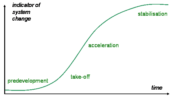
Figure 1. The four phases of a transition. The y-axis is an appropriate indicator of the system's change, and the x-axis is time. From Rotmans et al. (2001)

Transition pathways

2.7
In analysing transitions, it is useful to have a differentiated concept of transitions by 'type'. Different typologies have been suggested, e.g., by Geels and Schot (2007) and Smith et al. (2005). In our conceptual framework (Haxeltine et al. 2008) we use a hierarchy of terms to define a transition typology: a mechanism is a societal process integral to transition, triggered by another mechanism, or by an event. By 'event' we mean any occurrence which can have a major impact on the agents involved in a transition — i.e., the regime or the niches — such as interaction of two agents, landscape changes which weaken the regime, etc. A transition pathway is a minimal sequence of mechanisms and events needed to generate a transition, including a description of the initial and final states of the system. In this modelling exercise, we classify the transition pathways according to the events associated with them following the socio-technical transition typology of Geels and Schot (2007).

2.8
Geels and Schot base their transition pathway differentiation on two criteria: nature and timing of interactions. In respect of the nature of the interaction between the different levels, landscape (macro-level) changes can either reinforce the regime or put pressure on the regime, leading to change; similarly, niche (micro-level) innovations can compete with the regime, or they can have a symbiotic relationship with it. The timing of the interactions refers to how developed niche innovations are when landscape pressure appears.

2.9
Following the typology of Geels and Schot (2007), we attempt to model four transition pathways, summarised below: transformation, de-alignment and realignment, technological substitution, and reconfiguration. We will later attempt to model a simplified implementation of each of these pathways, following the historical examples of Geels and Schot (2007).

2.10
In the transformation pathway, moderate landscape pressure appears without significantly-developed niches in place. The incumbent regime adapts by adjusting its development and innovation in response to these pressures, seeking out new guiding principles and practices. This might include a power struggle, as the regime takes in nascent niche innovations. This pathway can, for example, represent a change instigated by a social movement.

2.11
If landscape change leads to a strong, sudden shock at a time when niche innovations are not developed, this leads to de-alignment and realignment. The regime erodes away and crumbles as actors lose faith, leading to a prolonged co-existence of multiple niche-regimes as innovations compete for resources and support. Ultimately, one will overpower the others and become the new regime, leading to re-stabilisation.

2.12
By contrast, in a technological substitution strong landscape pressure appears at a time when niche innovations are more developed. This alignment of the micro- and macro-levels allows a niche innovation to break through to the meso-level, growing and competing with the incumbent regime, and eventually replacing it. This pathway can portray an economic-technological story, where the regime actors are incumbent firms, and the niches newer firms inventing new technologies or functionalities, resulting in a market competition between the regime and the niches.

2.13
In a reconfiguration, niche innovations are developed and there is a symbiotic relation with the regime, which adopts some innovations. This can trigger further change: there is a recombination of old and new in the regime, and new behaviours and practices may be adopted at different levels. As landscape pressure continues, this leads to major reconfigurations in the regime through cumulative change, unlike the transformation pathway in which regime architecture is largely unchanged.

2.14
In the absence of (significant) landscape pressure, the regime will undergo incremental change only, and remain dominant in a reproduction process. Niche innovations may arise, but do not become powerful. The regime can be said to be dynamically stable.

* Model description

Background for our transition modelling

3.1
Drawing on the different theories and frameworks discussed above, we put together a conceptual framework for our transition modelling exercise (reported in detail in Haxeltine et al. 2008), which draws on both transition theory and social theory, as discussed above. The main features are:

3.2
In our modelling approach, we build on agent-based modelling, but our agents are complex sub-systems in themselves, and are potentially capable of more complex decision making. While we do not have a systems dynamics module included, we do combine our agents with systems dynamics thinking, in the interactions of agents with each other and with the landscape. In parallel model prototyping work we have considered a more economics-oriented model, using notions of utility maximisation by consumers (which we generalise to agents' attractiveness to consumers), following technological evolution models such as Schwoon (2005). In the model prototype reported upon here we take an aggregate approach to simulating individual niche and regime agents, but with individual citizens/consumers forming the support canvas. The notion of attractiveness is included in the model, and will be used in future to expand modules of individual decision making and/or market dynamics. Our conceptual framework, embedded in social theory and the emerging transitions theory, and using concepts of agent-based modelling and system dynamics is, we suggest, innovative and different from previous transition models.

3.3
Our general model is constructed as a prototype for researching transition pathways, and can be run as an abstract model with arbitrary parameters. For different implementations, the model is specified with appropriate parameterisations and rules. In the four transition pathways we present, we did not use extensive data. Basic data from the historical narrative is extracted in defining parameters and rules for the system, choosing regime and niches and calibrating their relative strengths, and defining societal support for different practices. A full case study would be more data heavy; however the type of model prototyped here is not designed for heavy computation or huge datasets, rather focusing on the changing dynamics of the system, using data to define the system's rules and components.

3.4
Our model prototype is implemented as a Java program that builds on the Mason library for agent-based simulation. It is operated within the Eclipse workbench, resulting in a powerful and user-friendly software environment. While our model so far is a prototype, we already consider ease of use and visualisation to make the model potentially accessible for a variety of users and stakeholders. The model is run in a 'transitions laboratory' pictured in Figure 2, with various options available at runtime, and also a variety of different visualisations. The outputs are graphs of selected parameters changing over time; one- or two- axis pictures of the sub-systems and supporters which change as the transition progresses (i.e., simple 'movies'); and logs of main events in the run, which help in analysis. We intentionally choose a few different types of graphics in presenting our results to show the versatility of visualisations.

Figure
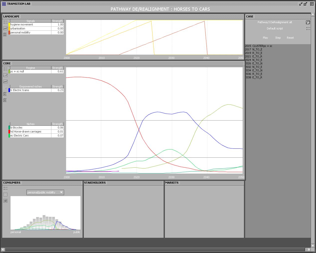
Figure 2. Our 'transition laboratory' in which the model is run, with various options at run time (click image for a larger version)

Model overview

3.5
We use a combination of agent-based modelling and systems dynamics modelling to capture transitions in socio-technical systems. There are a small number of complex agents, which have an internal systems dynamics model, and a larger number of simple agents. All agents and the systems are updated by timesteps. The model runs represent 50 years, with 600 timesteps, i.e., one timestep per month.

3.6
The sub-systems of regime and niches are implemented as aggregate agents, representing multiple actors. They have both a system dynamics internal structure, or metabolism, and agent-based modelling style interactions with other agents and the system. Agents rely on support for their strength; this comes from the support canvas, representing consumer/citizen support, implemented as supporters, which are simple agents. The (aggregate) agents and the supporters are set in a multi-dimensional practices space. Landscape pressure is implemented as external signals on the space, which can affect both agents and supporters. Figure 3 schematically shows a two-dimensional practices space, highlighting agents and supporters.

3.7
The agents have an internal metabolism, including structure and practices, with those of the regime dominant in the system. In the prototype, practices are each represented as values along two axes, constituting a two-dimensional practices space. Structure is quantified by each agent having stocks of physical capacity and institutional capacity. The structure requires resources, which the agent draws from the support canvas. The agent's institutional capacity also serves as its strength: its ability to influence other agents, the landscape, and the support canvas.

Figure Figure
Figure 3. Two illustrations of a two-dimensional practices space, with practice axes PX and PY. Left: regime and niches, which can move in the space and interact with each other. Right: the support canvas, showing supporters scattered in the practices space, coloured by the agent they support, red = regime (R), green = niche 1 (N1), blue = niche 2 (N2).

3.8
In this exercise, we choose two practices to capture an important part of each example; these are the axes of the practices space. Each agent is placed in the space according to the set of practices they represent. Supporters are placed in the practices space according to their preferences in the practice dimensions.

3.9
We define a transition as a fundamental change in the system's structure, culture and practices (Haxeltine et al. 2008). In the model implementation, we do not capture qualitative changes in structure, therefore we define a transition as a significant shift in the system's dominant culture and practices. In the model a transition can occur either through regime change, when one regime agent falls and a new regime agent arises with practices in a different location in the practices space, or through evolution (transformation) of the incumbent regime to a different location in the practice space. In the model, a regime 'falls' when its strength falls below a defined threshold. It could be immediately replaced by another agent which rises above the threshold, or there can be a period of no regime.

Agents

3.10
We represent the socio-technical system's regime and niches as aggregate agents in the model, i.e., representing multiple actors. While these are programmed as agents in the agent-based modelling sense, it is important to note that these are abstract entities, which do not exhibit agency in the social science sense. We therefore model them with simple behaviour rules in an attempt to capture elements of realistic behaviour of these sub-systems, rather than give them algorithms aimed at maximising strength or fitness.

3.11
We divide agents into three categories: niche, empowered niche agent (ENA), and regime. There can be only one regime at any time, although the system might have periods in which there is no regime. There may be zero, one or a few ENAs and several niches at once. We define the type of the agent by its strength with thresholds separating them (see transformation below). The regime is by definition the strongest agent and dominates the system, while niches have much less strength. We find it useful to define ENAs — niches which have grown strong enough to pose a potential threat to the regime, and therefore the regime's interaction with them is different from its interaction with niches. An agent's strength determines its behaviour (strategy), its interactions with other agents, and its attractiveness to supporters. In the simplest instance, without a system dynamics model, the strength of the agent equals its share of support from the support canvas. In this case, a regime is defined as an agent which has more than 0.5 (i.e., 50%) of the total support. However, in the full model, agents have an internal structure, or metabolism, which determines their strength, although this is ultimately dependent on support from the support canvas.

Agent movement

3.12
Each agent type (regime, niche, empowered niche agent) has a different behavioural algorithm for its movement in the practices space. The types we use are based on policy driven party dynamics of Laver (2005). The regime is an aggregator, adapting its practices to the centre of the consumer cloud in the practice space, in an attempt to maximise support. Laver has the aggregator attempting to aggregate its own supporters only. We add to this behaviour: when the regime's support falls below a threshold, it attempts to aggregate all consumers to increase its support. This attempts to capture the regime's tendency to be entrenched in its practices and to seek optimisation rather than innovation. ENAs are predators, moving their practices towards those of the largest agent, i.e., the regime, in an attempt to take support away from it. We depart from Laver in that in the absence of a regime, behaviour switches to hunter behaviour. Finally, niches are hunters, continuing movement in the same direction as long as their strength increases, otherwise moving randomly in another direction. Speed of movement is set by default at a ratio of 1:1.5:2.5 for regime, ENA and niche, respectively. This represents the higher inertia and entrenchment of larger agents.

3.13
In some cases, agent movement is limited in one or more practice axes by frontiers. An agent approaching a frontier moves slower and slower. A frontier may apply to one, some or all agents, and may change during the run. They may represent technological limitations, e.g., in one of our examples sailing ships cannot deliver as fast as steam ships due to technological differences; or cultural imperatives, e.g. in another example a hygiene movement cannot, by definition, have a practice representing poor hygiene.

Inter-agent dynamics

3.14
Besides handling their internal metabolism and coping with the landscape, agents interact with each other, and this plays an important role in model dynamics. We classify this behaviour as mechanisms, involving agent dynamics or interactions between agents. The model explicitly includes the list of mechanisms detailed below. The notion of mechanisms is further detailed in Haxeltine et al. (2008).

3.15
Niche agents try to survive and grow in a landscape dominated by the regime, which is more powerful than they are. If they have similar practices to the regime, they find it hard to gather support in its shadow, but if they are too innovative or otherwise far from the regime's location in the practices space, they will find the support canvas too sparsely populated for strong support. Niches can grow by clustering (merging) with other similar niches, or by biding their time until landscape changes favours them over the regime. Two niches i and j might cluster if they are close to each other in the practices space and are moving in a similar direction. I.e., there is a possibility of clustering if the (normalised) distance between them is less than Dmax (set to 0.15 by default) and the angle between their current directions of movement is less than anglemax (set at 0.2π-0.5π). The probability is set to:

pi,j = c(1-Di,j) (1)

where c is the clustering parameter, set to 0.2 by default. When two niches cluster, the resulting agent (niche or ENA if its strength is above the T1 threshold) has the sum of their structure parameters PC and IC, and the average of their locations in the practices space.

3.16
The regime can attempt to adapt its practices gradually through adaptation, but also through taking up some practices of innovative niches, via absorption of one or more niches. If this mechanism is used, the regime will attempt to absorb any niche located in the area of the practices space towards which the regime is heading. Similarly to the clustering mechanism, absorption is defined by distance and a maximum angle (set at 0.15π-0.2π), although here the angle is between the movement direction of the regime and the location of the niche relative to the regime. The probability of absorption of niche n by regime r is then:

pr,n= c(1-1.2Dr,n) (2)

using the same c as the clustering parameter, set to 0.2 by default. The reduction of the probability of absorption at greater distances and the maximum distance at which a niche can be absorbed both express the regime's limited ability to change. Similarly to clustering, the resulting (regime) agent after absorption has the sum of the structure parameters and the average of the locations of the original agents. While the first makes a small difference to the regime, the second allows it to take a big step in the direction it was heading in the practices space, and is much faster than adaptation.

3.17
Niches emerge in an area of the space where there are 'dissatisfied' supporters, i.e., where there are supporters and no nearby agent. Our algorithm implies that an entrepreneurial supporter (representing an individual or small group of citizens or consumers) which is not satisfied with the existing agents forms a new niche. For the emergence (birth) of niches, we define a dissatisfaction parameter based on the distance of the nearest agent from the supporter, this is the cumulative dissatisfaction level (CDLC):

CDLCt= m.CDLCt-1+(1-m)DCt (3)

where DC is the distance to the nearest agent, and m represents the supporter's 'memory' of previous (dis)satisfaction. For each supporter, the normalised CDLC determines the probability of a niche emerging at the supporter's location. For supporter i the probability of a niche emerging at each timestep is:

pi = b.CDLCi /CDLCmean (4)

where b is the birth parameter, set to 0.01 by default.

3.18
We define a transformation as an agent crossing a strength threshold and thereby changing from one type of agent to another. When several niches cluster together, or when a niche gains enough strength to cross T1, it becomes an empowered niche agent (ENA). By 'empowered' we mean that the niche is now powerful enough to be thought of as a potential threat to the regime's dominance, thereby changing the inter-agent dynamics. Unlike a niche, an ENA cannot be absorbed by the regime. An ENA whose strength goes below T1 transforms into a niche. If the regime goes below strength threshold T2, it is deposed and becomes an ENA. In the lack of a regime, an ENA exceeding T2 becomes a new regime. Our default values are T1 = 0.15 and T2 = 0.5, i.e., 15% and 50% of the total strength in the system, respectively.

Transitions in the model

3.19
As stated above, there are two ways a transition can be represented in the model. The first is regime change, which occurs when an incumbent regime loses support and ultimately strength, falling below the T2 threshold, and an ENA with different practices takes its place, gaining strength and exceeding the T2 threshold to transform into the new regime. Unless the replacement is immediate, there will be a period of no regime in between. While the old regime could theoretically become reinstalled, model dynamics make this unlikely. Regime change is found in the technological substitution and de-alignment/realignment pathways. The second is regime evolution, which occurs when the regime significantly changes its practices through adaptation and/or absorption of niches, moving to a different location in the practices space. In this case, we need to define indicators as to how much change in the system would constitute a transition.

Internal structure — agent metabolism

3.20
Every agent has a metabolism — the repeated gathering, allocation and spending of resources. The resource flow is spent on the structure stocks of institutional capacity and physical capacity, and agents choose how to allocate the resources between the two. Institutional capacity (IC) expresses networks of business, industry, politicians, lobbyists and other actors. The regime has high IC, representing a large network, which results in a high institutional inertia, i.e., rigidity and resistance to innovation and radical change. Niches have smaller networks of actors. In model terms, IC is used to represent the agents' strength. Physical capacity (PC) expresses physical infrastructure, technical capability, physical and knowledge capital, and production capacity. In model terms, PC limits resource generation. The regime has high PC, representing the large physical infrastructure, high production and use capacity, and technological and knowledge capital. Niches have lower or incomplete infrastructure or capacity. Both IC and PC undergo depreciation over time, and must be 'topped up' by resource allocation. The agents' metabolism as part of their internal structure is illustrated in Figure 4.

Figure
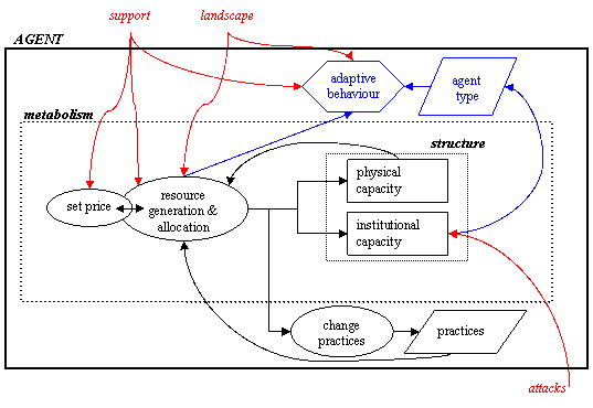
Figure 4. Agent metabolism as part of the agent. Resource gathering depends on external support and landscape, and internally on price, physical capacity and practices. Resources are spent on physical and institutional capacity, as well as on adaptation through changing practices. Institutional capacity in turn determines the type of the agent (niche, ENA, or regime); it can be reduced through external attacks.

3.21
Resource generation depends on the agent's support and its production (physical) capacity, but can also be influenced by landscape signals and policy events. By resources we mean cash flow and investment. The agent's resource generation is a simple production function including output (goods value) and price, assuming a constant ratio of price to cost:

R = price . output (5)

where R is resources. We define output as:

output = min(PC + 0.5, support.CONSTsupport) (6)

where PC is physical capacity. The constant is calibrated to match a 'healthy' regime with support = 0.8 and physical capacity PC = 100, so CONSTsupport = 125. The full resource equation includes miscellaneous effects of landscape and policy as well:

R = price . output . f(landscape,policy) (7)

Physical and Institutional capacity are calculated by depreciation d and an addition from resources:

PCt = PCt-1(1-d)+CONSTPC.R.fPC (8)

ICt = ICt-1(1-d)+CONSTIC.R.fIC (9)

where fPC and fIC are the allocation fraction of resources to PC and IC, respectively.

Resource allocation

3.22
The metabolism diagram (Figure 4) shows several possible uses for resources: maintenance and expansion of physical capacity (PC) or institutional capacity (IC), or adapting i.e., moving in the practices space by changing practices. The default model assumes an equal division of 1/3 of resources for each of these three. I.e., 1/3 of resources are assumed to be spent on adaptation regardless of how much the agent has moved in the practices space in each timestep, and the rest is spent equally between PC and IC, i.e., fPC = fIC = 0.33 in equations (8) and (9).We have also considered more sophisticated agent behaviour, in which the agent can choose to stick to its practices and spend all resources on structure, i.e., fPC = fIC = 0.5. Finally, we experimented with the possibility of an agent increasing allocation of resources to PC at the expense of IC and vice versa (If physical capacity limits resources (6), a larger share is diverted to PC, and if institutional capacity is low more is diverted to IC). However, the last two options involved more complex decision making and did not have a significant impact on model dynamics or results, so the default three-way equal split was used in all runs.

Supporters and support canvas

3.23
The support canvas aims to internalise some parts of the landscape, such as social trends. In this model, we implement the support canvas to represent individual supporters, which can be thought of as consumers, citizens or other small scale actors. The supporters are scattered individually in the model's practices space. A supporter's location in the practices space indicates its ideal points, preferred practices, or best expectations of practices from the agents. The supporters are implemented as simple agents, which perform two functions. First, at each timestep they support ('vote for') one aggregate agent (the regime, a niche, or an empowered niche). Support is determined by the agents' relative attractiveness (see 3.25), and is ultimately the agents' source of strength. Second, supporters move in the practices space when landscape signals are present (see 3.29).

3.24
We use 1,000 or a few thousand supporter agents in the model, representing in some cases millions of citizens, consumers or small groups of actors, as it was found that a larger number of supporters did not change model dynamics. The placement of supporters in the practices space is in one or more groups. Each group is scattered in a normal distribution around one location. At the start of a run, the regime will normally be located near the centre of the largest group of supporters, and receive most of the support. The groups are used for initial location of supporters only; we do not implement any social networks between the supporters.

Attractiveness function

3.25
The attractiveness function determines which agent the supporter will support. At each timestep, every supporter chooses to support the agent which has the highest attractiveness (for that supporter). This is determined primarily by two considerations: the strength of the agent (see above), and the match between the supporter's ideal practices and the practices of the agent. This match is expressed as the distance between the two in the practices space. This suggests the following attractiveness of agent j to supporter i:

attractivenessi,j = α.sj -Di,j2 (10)

where s is the agent's normalised strength, D is the normalised distance between the supporter and the agent, and α is the relative weight of the agent's strength, set between 0 and 1. A value of α = 1 would indicate that the strength of the agent was a major factor, whereas a value of α = 0 would indicate that satisfaction with the agent was the only consideration. The default value is α = 0.05. We replace the distance with an ongoing measure of the supporter's satisfaction with the agent over time. We measure the cumulative dissatisfaction level (CDL) as the previous dissatisfaction level combined with normalised distance:

CDLt = m . CDLt-1 + (1-m)Dt (11)

where m represents the supporter's 'memory' of previous (dis)satisfaction. The default value for m is 0.5. The attractiveness function over time is therefore:

attractivenessi,j = α.sj -CDLi,j2 (12)

Finally, we consider 'miscellaneous' effects which change supporters' views and choices, which could include prices, or socio-political considerations which are not captured in the practices space. This gives us:

attractivenessi,j = α.sj -CDLi,j2 +Impi.Effj (13)

where Eff is the effect value for agent j, and Imp is the importance of the effect for supporter i.

Landscape

3.26
The landscape, or macro-level, is an expression of slow changing world views and paradigms, macro-economy and material infrastructure, as well as the natural environment and demographics. In the model we express the landscape partly as the support canvas (see 3.23) and partly as external signals. These signals can have a few different effects: the default use in the model is to change supporters' preferences, causing them to move around the practices space (see 3.29, 3.30). Each signal is a vector, i.e., it has a strength and a direction in the practices space, which determine its push on the supporters. This plays an important part in the dynamics of the model, as the changing locations of the supporters force the agents to adapt or lose support and power. This does not imply that the transitions are necessarily 'consumer led': the change in supporters' preferences is part of the system as a whole changing, an internalised part of the landscape.

3.27
Another way in which landscape signals are used is to directly affect agents in various ways, e.g., changing resource gathering potential for a given set of practices, which can strengthen or weaken the agents, or weakening the attractiveness of a certain agent, e.g., the hygiene movement reducing the attractiveness of horse-based urban transport in the transport transition example.

3.28
Complementing landscape, in some runs we include specific policy events. These are events that reflect specific policy decisions rather than broader landscape changes. An example of a policy event is lowering prices for one or more agents through subsidies, which could either raise the attractiveness of the agent(s) or give the agent(s) more resources per supporter.

Movement

3.29
Supporters move around the practices space over time, as changes in the landscape change their preferences. This plays an important part in the dynamics of the model, as the changing locations of the supporters force the agents to adapt or lose support and power. At each timestep, each individual supporter has a probability of moving, set by default to 0.01, i.e., there is a 1% chance of each supporter changing preferences at each timestep.

Table 1: Model timestep summary: the actions, in order, at each timestep of the model

Action Sub-actions Notes
Landscape. update signals/policy eventsupdate the landscape signals, from which the pressure field is calculated
Metabolism. set IC
. set PC
. set output
. set price
. set resources
for each agent, calculate the metabolism parameters from support and other parameter values
Normalise. set normalised strengthset strength of each agent to normalised IC
Supporters. move
. set distances
. set CDLs
. choose agent to support
. calculate probability/direction of move from pressure field
. calculate distances from agents' locations
. calculate CDL from distances and previous CDL
Agents' Movement. decide strategy
. move
. set strategy by agent type
. move by strategy
Mechanisms. birth
. absorption
. clustering
. transform 1
. transform 2
activate all that are appropriate

3.30
If a supporter moves, the strength and direction of their movement is determined by a pressure field, which is calculated from the landscape signals (see 3.26). The strength with which a given landscape signal pushes a supporter is determined separately for each axis, and is a function of the strength of the signal in that direction and the location of the supporter on the axis. The push lessens up the axis in the direction the signal is pushing, e.g., a push to higher hygienic standards will have less effect on supporters who already support highly hygienic practices. In the 'lower half' of the axis the push is full strength, dropping linearly to 0 for the 'upper half'. For example, a landscape signal has a strength of 1.0 along the x-axis, which has possible values (-100,100). The strength of the push in the x direction is 1.0 for supporters located at x <= 0, dropping linearly to 0.5 at x = 50, and to 0 at x = 100. The total push of each landscape signal is a vector of the landscape signal's push along each practice axis, and the pressure field is the vector sum of the landscape signal pushes.

3.31
A summary of all the actions occurring at each timestep of the model, in order, is in Table 1.

* Modelling transition pathways

4.1
In this modelling exercise, we demonstrate each of the four transition pathways in the taxonomy of Geels and Schot (2007). We do this by using a simplified version of the historical example they give for each pathway. Our aim is not to reproduce the full historical transition story, but to distil from the historical examples the most important points needed to demonstrate the transition pathway associated with it. For that purpose, we define a regime and one or more niches for the pathway; we choose two practice axes; and we define landscape signals and other essentials to capture the pathway. We introduce each run with a brief outline of the historical example, followed by the model parameters chosen to represent that pathway and our criteria for successfully modelling the given pathway.

Transformation pathway

4.2
As an example of the transformation pathway, we look at The Netherlands, 1850-1900: the Dutch public hygiene transition from cesspools to sewer systems show a transformation, with some elements of technological innovation (Geels and Schot 2007). In the 1850s there was pressure on the regime from hygienist doctors (outsiders), who demanded better treatment of sewerage: correlations were found between disease and environment, e.g., overflowing cesspools. The regime played down the importance of these findings, and made some incremental changes (improvements, not systemic changes); health was seen as a personal issue, not one for the authorities. In the 1870s and 1880s, the landscape changed as industrialisation brought more workers to the cities, who often lived in filthy areas without sanitary facilities. The pressure from doctors on the regime continued, partly as doctors teamed up with engineers. Following this increased pressure, and Pasteur's theory of micro-organisms, which explained the spread of infectious diseases, a hygiene movement emerged. The regime responded by altering goals, and making some changes to practices, but these were insufficient to solve the problems. By the 1890s norms had changed, with cleanliness becoming a widespread cultural value. Also, democratisation gave incentives for local government to take working class needs into consideration. This lead to more encompassing solutions, with sewer systems built in The Hague in 1893, and later in Amsterdam in 1914.

4.3
We implemented this example as specified in Table 2. We define two agents — the regime of local government and departments of public works, and a niche originally of hygiene doctors and later becoming a hygiene movement. The practice axes chosen were a hygiene axis (efficiency of waste disposal practices) and a democratisation axis (public versus personal responsibility for health). Niche 1 has a frontier — limiting it to high values on the hygiene practice, required by it being a hygiene movement niche. The mechanisms in the transition are adaptation of the regime to the changing landscape, and possibly absorption of the niche by the regime. Birth and clustering were not used in these runs, and transformation (e.g., of niche to ENA) is not expected if the historical pathway is captured. The chosen landscape signals are urbanisation, which increases pressure on the sanitary system, which is represented as a weak push of supporters up the hygiene practice axis (axis 1); change in norms of hygiene, resulting in a stronger push on axis 1 and a slight push on axis 2; and democratisation, represented as a stronger push up axis 2.

Table 2: Model setup for the transformation pathway

Example 1: cesspools to sewer systems, The Netherlands, 1850-1900
AgentsRegimelocal government, departments of public works
Niche 1hygienist doctors / hygiene movement
frontiers: limited to high hygiene and public responsibility (i.e., high values on practices 1 and 2)
PracticesAxis 1efficiency/hygiene of waste disposal practices
Axis 2role of authorities in public life (individual v public responsibility for health)
FrontiersNiche 1limited to high values in practice 1 (i.e., a niche of hygienist doctors or a hygiene movement necessarily demands high hygiene standards)
MechanismsAdaptationregime expected to adapt its practices considerably
Absorptionregime expected to absorb the hygiene niche
Landscape signals1urbanisation following industrialisation (more pressure on the hygiene systems)
effect: slow supporter movement up practice 1, 1865-1890
2norms of hygiene increase
effect: increasing supporter movement up practice 1,
slow supporter movement up practice 2, 1850-1890
3democratisation and more public responsibility
effect: strong supporter movement on practice 2, slight movement on practice 1, 1880-1890

4.4
While some new technologies are included in this example, it is primarily a transformation transition, with the regime adapting to changing landscape conditions. A transition in this example will be either regime change, with the hygiene movement becoming the new regime, or a transformation of the regime, through adaptation of practices and/or absorption of the niche and adopting its practices. In order to judge whether the transformation transition was successful (when there is no regime change), we will look at the change in practices of the regime, i.e., how far it moves in the practices space.

De-alignment and Realignment pathway

4.5
As an example of de-alignment and realignment, we look at the US in the 1880s - 1920s, where a transition took place in urban transport from horse-drawn carriages to automobiles (Geels and Schot 2007). This transition shows a de-alignment and realignment pathway, with two subsequent technological substitutions. In the late 19th century American society was in flux due to changes including the hygiene movement, urbanisation, electricity as pervasive technology, and an expanding middle class. This was a period of opportunity for niche innovations, as pressures mounted on the horse-based urban transport regime: the hygiene movement raised concerns over horse excrement, urban expansion led to longer travel distances, and there was a high cost to keeping so many horses in the cities. Electric trams benefited from electricity, supported by powerful actors (utility companies), and became the first technological substitution. Other options appeared as well, such as the safety bicycle in 1885. Different types of cars appeared in the 1890s, as small but visible niches, including taxis, luxury rides, racing, and touring niches. In 1908-1916 T-Ford's mass production brought car prices down, leading to competition between electric trams and (petrol) cars. By the 1920s, cars supported by powerful actors overtook trams in the second technological substitution.

Table 3: Model setup for the de-alignment / realignment pathway

Example 2: horses to carriages, USA 1870-1920
AgentsRegimeHorse drawn carriages and trams
Niche 1electric trams
Niche 2bicycles
Niche 3electric cars
Niche 4petrol cars
Niche 5steam engine cars
PracticesAxis 1personal mobility v public mobility
Axis 2length of commuting / day-to-day trips
FrontiersAllAll agents are limited in their movement from their original positions, as the practices refer largely to the nature of the technology and infrastructure of each mode of transport.
MechanismsClusteringused in some runs — different car niches expected to cluster
Landscape signals1hygiene movement (problems with horses)
effect: lowers attractiveness of regime, reaching maximum at 1890
2(sub)urbanisation
effect: increases average length of commute and day-to-day trips, i.e., movement up practice 2, 1870-1895.
3increase in personal mobility (following success of cars and bicycles)
effect: supporter movement down practice 1, 1885-1910
4technological innovation — electricity: reduced price of trams 1880-1900
5technological innovation — mass production: reduced car prices 1890-1910

4.6
We implemented this example into the model as specified in Table 3. While some adaptation is expected here, and possibly clustering of the different car niches, the major events in this transition are the crumbling of the existing regime, due to landscape signal 1, followed by competition between different niches, and their growing metabolism and relative attractiveness determining which will replace the original regime. The attractiveness function here includes the effects of lowering attractiveness of horse-based transport due to hygiene norms changing (landscape signal 1), and in some runs the effects of electricity and production lines lowering the price of trams and cars, respectively. Equation (13) was amended as follows:

attractivenessi,j = α.sj - CDLi,j2 +ImphygieneEffhygiene,j + Impprice(1-pricej) (14)

It was assumed for simplicity that the importance of the effects was the same for all supporters, and the values were set at Imphygiene= 0.15 and Impprice = 0.05. Effhygiene rises linearly from 0 in 1870 to a maximum of 1 in 1890 for horse-based transport, and is 0 for all other agents. Price was set to 1 by default for all agents. In some runs, the price for electric trams was set at 2 at the beginning of the simulation and the price of all cars at 5; the prices then dropped either linearly or suddenly to 1 (dynamic learning curves were not included). The success of the transition here would be in regime change. It will be judged to be a de-alignment / realignment pathway if support disperses among various agents when the original regime collapses, and two or more niches compete for supremacy after the collapse, rather than one regime quickly replacing another.

Technological Substitution pathway

4.7
For the technological substitution pathway, we look at the British transition from sailing ships to steam ships, ca. 1840-1920 (Geels and Schot 2007), although for consistency we keep the 50-year model run, defining it as 1850-1900. This was a technological substitution, with a technology push and crucial landscape changes. In 1838 a subsidised market appeared for mail steamers, which were expensive but faster and had more reliable schedules than sailing ships. This resulted in a niche of steamship builders. Later, high wages in the USA, political revolutions, and the Irish potato famine (1845-1849) resulted in a mass increase in emigration from Europe to America, boosting the trans-Atlantic passenger market from the 1840s onwards. Larger steamships could take advantage of this due to technical improvements. Crucially, the Suez Canal opened in 1869: sailing ships couldn't use it, giving steam ships a great advantage with shorter routes to India and China. Over the period 1870-1890 steamships out-competed sailing ships in passenger markets. Larger ships, improved marine steam engine efficiency and economies of scale allowed this to happen, and socio-technical change accompanied the transition, with larger ports and a global coal infrastructure. Sailing ships attempted improvements with larger ships, as well as more substantial changes such as using iron and mechanising equipment, but ultimately could not compete with the efficiency of steam ships. Nonetheless, these improvements allowed sailing ships to survive for a long time, where price was the main factor in choice of technology: they had the advantage of price not increasing greatly with distance, in contrast to the steamships.

4.8
We implemented this example into the model as described in Table 4. The practices chosen — speed/reliability and price — required a variation of our attractiveness function: while the supporter's location in the practices space may indicate their expectations, we assume that no supporter would object to a cheaper fare or a more reliable and faster mode of transport. When calculating distance in the practices space, that distance where the agent offers something 'better' than the supporter's location is ignored. The effect of the offer of an improved service is not internalised in the current model; i.e., there is no closed circuit of preferences changing with a 'better' offer; in this example we include this artificially with landscape signal 3. In addition, this offers a feedback between the practices and the metabolism, as prices affect resource generation. This feedback has not been fully explored. Success of a transition will be in the transformation of the steamships niche into a new regime, with practices different from those of the original regime. Finally, in this example ENA behaviour is set to hunt rather than predate, as it seems unlikely that as steamships become a more powerful niche, they will resort to being slower and less efficient in an attempt to capture support from the sailing ship regime!

Table 4: Model setup for the technological substitution pathway

Example 3: sailing ships to steamships, Britain 1850-1900
AgentsRegimeSailing ships
Niche 1Steam ships
PracticesAxis 1speed & reliability
Axis 2price
FrontiersRegimeSailing ships have limited room for improvement of speed and reliability, as is represented by a frontier of this practice.
MechanismsAdaptationadaptation of the steamship niche — becoming more reliable and eventually cheaper — play a major role in this pathway.
TransformationThe steam ship niche is expected to transform from niche to ENA, then to regime. The incumbent regime of sailing ships expected to transform down to ENA, and perhaps niche.
Landscape signals1emigration = increased passengers
effect: increased demand for fast, reliable transport, i.e., supporters move up practice 1
2Suez Canal opening
effect: step function in 1869 which increases steam ships' speed and reduces their price.
3increased business expectations for cheap, fast transport
effect: moves supporters up practice 1, and a little bit down practice 2

Reconfiguration pathway

4.9
The example we take for the reconfiguration pathway is the American transition from traditional factories to mass production, ca. 1850-1920. This transition involved interactions between multiple component innovations and the regime. In the 1850s and 1860s, there appeared a division of labour and mechanisation through application of machine tools. General purpose tools, such as turret lathes and planers increased productivity and could be operated by semi- and unskilled labour, increasing output efficiency and reducing labour costs. These were powered by steam engines via belts and pulleys, with some loss of energy through friction. In the 1860s and 1870s some industries introduced 'continuous movement' via endless chains or moving benches, further increasing efficiency, while in other industries small battery powered electric motors appeared. In the 1880s and 1890s special purpose machine tools enabled production of precise interchangeable parts, further speeding up assembly. However, the expanding scale and number of machine tools resulted in problems with factory layouts. Niche innovations began to enter the regime: e.g., combination machine tools and conveyor belts. Soon electricity entered factories, becoming a pervasive technology: in 1899, 5% of aggregate power in American industry supplied by electric motors, this rose to 25% in 1909. At the beginning of the 20th century layouts of factories changed, as efficient throughput became an important guiding principles.

4.10
We model the reconfiguration pathway without using specific pre-programmed innovations, but rather by the birth of new niches as an internal dynamic in the model, see Table 5. The landscape changes offer new possibilities, moving the ideal points of supporters as electricity, the efficiency movement and the rise of professional engineers yield various innovations. This implicitly assumes that the supporters in this pathway are not only consumers, but also various actors involved in industry. While this approach makes this example more abstract, it allows the reconfiguration to emerge as a more organic process; innovations emerge as the landscape changes, but this does not guarantee that the regime will keep up with the changes through reconfiguration or simple adaptation.

4.11
Defining the transition here is simply looking at the distance the regime travels during the run, i.e. how much its practices change. However, to distinguish a reconfiguration transition from a transformation, we require that the regime absorb more than one niche in addition to its adaptation.

Table 5: Model setup for the reconfiguration pathway

Example 4: traditional factories to mass production, USA 1850-1900
AgentsRegime(starts as) traditional factories
Nichesnone at start; birth of niches as new innovations appear.
PracticesAxis 1organisation of production (including power source — water / steam / electricity; individual craftsmen / craft workshops / production lines)
Axis 2mechanisation and division of labour
MechanismsBirthvarious improvements expressed as the emergence of new niches.
Absorptionthe regime expected to absorb niches as it assimilates new ideas and changes its practices
Landscape signals

1Electricity as pervasive technology (enables more mechanisation and electricity as power source)
effect: moves supporters a lot up practice 1 and a little up practice 2
2The Efficiency Movement (increasing production lines and division of labour)
effect: moves supporters a lot up practice 2 and a little up practice 1
3The rise of professional engineers and industrial managers and accountants (increasing organisation and division of labour)
effect: moves supporters up practice 1 and practice 2

* Results and analysis

5.1
Each of the four examples detailed above was run at least one hundred times to check the behaviour of the model and its ability to capture the different transition pathways, and to see how well the simplified historical transitions could be captured. Besides these results, we also show a summary of results from separate work (Köhler and Schilperoord unpublished), in which we took a more in-depth look at the sail-to-steam example. The basic results are followed by a more general analysis.

Transformation pathway

5.2
In the first example, support slowly turns from existing practices of low hygiene and low public responsibility to high hygiene norms and increased public responsibility. Model runs could be clearly divided into two groups: those with niche absorption, and those without. In the former, the small hygiene movement niche started to grow, but was then absorbed by the regime, as the latter sought to improve its practices. In these runs, the overall practices of the regime changed considerably on both axes, partly through direct adaptation, and partly through the absorption of the hygiene movement niche. Figures 5a and 5b show the changes in the supporter 'cloud' and the regime adaptation in a typical run, and Figure 6a shows a typical strength profile over time for such a run. The growing support for the hygiene movement, followed by small changes in the regimes practices, and ultimately the absorption of the niche by the regime and more substantial practice changes are a good qualitative match for the historical case study, and meet our criteria for a transformation pathway transition.

Figure
Figure
Figure
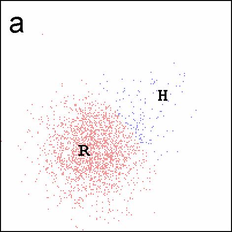
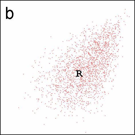
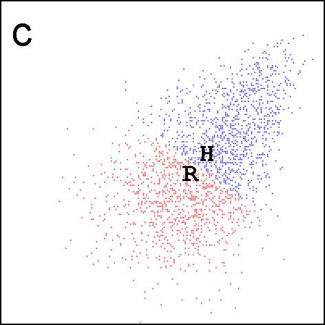
Figure 5. Supporters and agents in the practices space in example 1: the x- and y-axes are practices 1 and 2, respectively; supporters are located at their ideal practices, and marked as dots, coloured red if they support the original regime and blue if they support the hygiene movement; R marks the position of the original regime agent, H that of the hygiene movement agent. The three panels show the beginning of a run (a), the end of a run with absorption (b) and the end of a run without absorption (c).

5.3
In runs in which the hygiene movement was not absorbed, competition emerged between the two agents. Over time, more and more support switched from the incumbent regime to the hygiene movement, until it became an empowered niche agent (ENA). While the hygiene movement gained support quickly, it took more time for it to gain strength, because of an initially low institutional and physical capacity. The difference between support and strength acts as a dampening mechanism here. Eventually, the hygiene movement emerged victorious and deposed the regime towards the end of the run (Figure 6b), constituting a substitution transition, rather than a transformation. We stress that these runs are not 'wrong', but represent a plausible alternative scenario to the historical one in our simplified story, i.e. the rise of a new regime from the hygiene movement. However, another problem presented itself here: when the old regime was deposed, it remained an ENA, and then pursued the hygiene movement, following the 'predate' behaviour algorithm. This resulted in the two agents having almost exactly the same practices at the end of the run (see Figure 5c), which is difficult to interpret as a plausible history; it must be seen as an artefact of the model, and the behaviour of the ENA must be improved, or a frontier added to limit the movement of the original regime. The problem did not emerge when the hygiene movement became an ENA, since its frontiers did not permit it to completely take on the regime's practices.

5.4
In calibrating the model, we found that the angle for absorption (see 3.16) changed the absorption probability considerably: at a large angle of 0.2π the niche was absorbed in 96% of the runs, dropping to 29% at an angle of 0.15π. The higher absorption rate in runs with the wider angle makes it a better match for the historical case study. However, at the wider angle the niche was absorbed in the first ten years of the simulation (i.e., by 1860) in over 80% of the runs, which does not match the case study. At the narrower angle this happened in only 35% of the runs in which the niche was absorbed. Smaller angles make absorption unlikely until the regime is 'in trouble' and moving decidedly in one direction, towards the niche; however, we do not attribute significance to the exact angle in this qualitative reconstruction. A possible development for future modelling is fine tuning of the absorption mechanism: rather than being 'on' or 'off', the chances for absorption could change during the simulation, e.g., the angle could be increased when the regime loses strength or support and becomes more desperate.

Figure
Figure
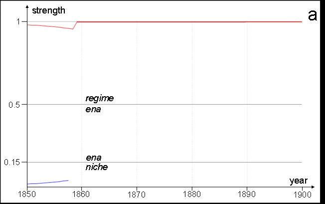
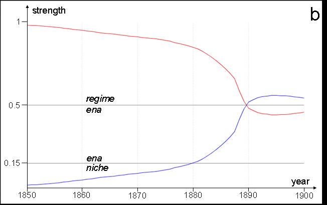
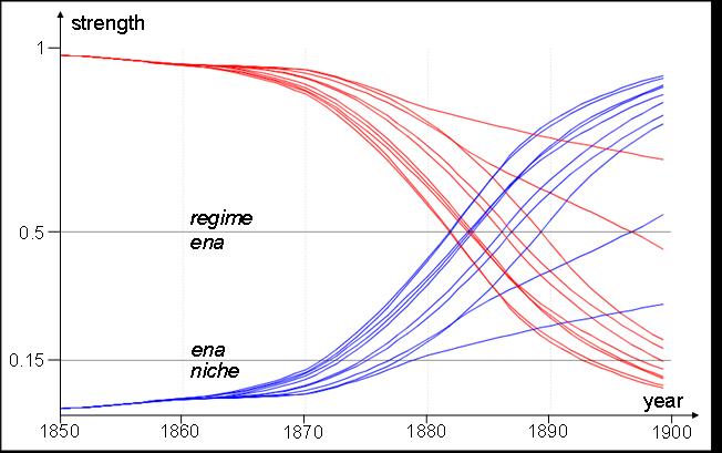
Figure 6. Normalised agent strengths in example 1: a run with absorption (a) and one without (b). The x-axis is time (years), the y-axis normalised strength, with vertical sections differentiating niches (bottom), ENAs (middle) and regime (top). The red line is the original regime agent, the blue is the hygiene movement agent.

De-alignment and Realignment pathway

5.5
In the second example (horse-based transport to cars), all runs showed the system switching away from horse-based transport. In over 90% of the runs, cars of one or more type became a stable regime by the end of the transition. Trams play an important role earlier in the simulation, becoming an interim regime in approximately 75% of the runs. However, the dynamics of the runs varied considerably with different patterns emerging, and were very sensitive to choice of mechanisms and parameterisation. The detail of our model example is not enough to catch the full history of this transition, as is made clear from the fact that electric cars usually become the new regime, rather than petrol cars; our choice of practices makes electric cars take off first in most runs, making it difficult for the other car niches to gain support. On the other hand, the overall dynamics of the simulations capture the de-alignment and realignment pathway well in the diversity of agents after the horse-based transport regime collapses, and the presence of an interim tram regime is a good match for the historical example.

5.6
Runs without the price effect on cars and trams showed various niches gaining support as horse-based transport became less attractive. In over 80% of these runs, trams and electric cars were neck in neck gaining strength as the old regime collapsed, both becoming ENAs. While the trams gained the most support, both of these agents were limited for a while by their physical capacity as they grew, hence the stiff competition. In nearly all runs, electric cars later became more powerful as supporters' preferences changed, and deposed trams to become a new regime. Figure 7a shows one such run: as the old regime collapses, trams and electric cars take off, and some other niches gain a little bit of support as well. Figure 8 shows supporters' distribution on each axis in this run, and it is evident that at the end of the run, there is still support for a variety of agents, despite electric cars being a stable regime. In approximately 25% of these runs, electric cars managed to out-compete trams and become the new regime much earlier. We also tried some runs where the metabolism was switched off, and strength was based solely on support. In these runs, the horse-based regime collapsed very quickly and trams became the new regime just as fast, with little growth in other niches; electric cars replaced trams later, also very quickly.

Figure
Figure
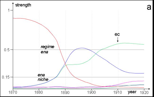
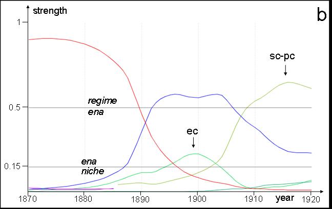
Figure 7. Normalised agent strengths in example 2: without price effects (a) and with sudden price changes (b). The x-axis is time (years), the y-axis strength, with vertical sections differentiating niches (bottom), ENAs (middle) and regime (top). The red is horse-based transport, blue = electric trams, light green (ec) = electric cars, pink = petrol cars, olive green (sc-pc, in b only) = cluster of steam and petrol cars.

Figure
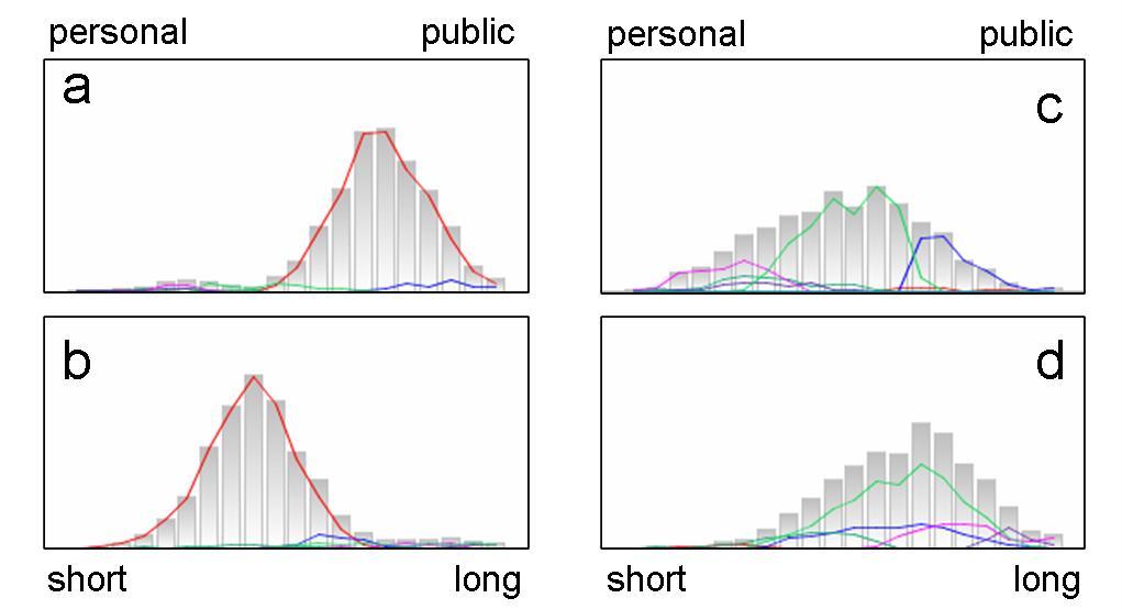
Figure 8. Supporter preference distribution in a typical run of example 2: the x-axis shows (discrete) ideal points for the practice, bars show number of supporters with that ideal point. Coloured lines show strength of support for different agents by ideal practices. Distribution is shown at the beginning (a, b) and end (c, d) of a run, for personal/public mobility preference (a, c), and average length of day-to-day trips (b, d). At the beginning of the run supporters tend to favour public mobility over personal, and have fairly short day-today trips, with almost all choosing horse-based transport (red). At the end of a run there is more personal mobility and longer trips, with most supporters favouring electric cars (green), but some preferring trams (blue), petrol cars (pink) or other modes of transport.

5.7
Including the price effect changed the system's dynamics, although usually not the outcome of the runs. When the price change was a step-change, the high price of cars when horse-drawn transport collapsed led to trams quickly becoming a regime in over 90% of runs. Trams were later deposed by cars as the cars' price fell and preferences changed. When price changes were made gradual, cars put up more of a fight in the early days. In all cases, bicycles managed to attract some support, especially when regimes fell; however, their strength never rose very high. Figure 7b shows an example run with step change prices, in which a niche cluster of steam and petrol cars becomes the new regime.

5.8
In some runs, the niche clustering mechanism was included; the location of the agents in the practice space meant that effectively only two or all three of the car niches could cluster, usually the steam and petrol niches. This does not represent a merging of technologies, but a coming together of the actors in these niches, sharing similar infrastructure and offering similar services, products and otherwise a similar market, with one or more technologies available. In these runs, the steam/petrol cluster competed with electric cars — sometimes one becoming the regime, sometimes the other, and in some cases there was no regime at the end of the run, only one or more ENAs.

Technological Substitution pathway

5.9
In the third example, we found that a technological substitution, where one agent becomes a new regime and deposes the old, was easily captured in this model. However, the details of the historical example are more difficult to capture. In this pathway, price was treated as a practice, rather than an integral part of the metabolism, leading to unrealistic dynamics of higher prices despite lower costs. Results showed that in 80% of runs the steamship niche easily out-competed the sailing ships over time, becoming an ENA approximately halfway through the run, and later a regime, as its practices improved and landscape signals favoured it. In a minority of runs the progress was slower, but increasing support for steamships near the end showed it would inevitably win out given enough time. Figure 9 shows a batch of ten runs for this example. In separate work (Köhler and Schilperoord unpublished, see 5.14- 5.17) we show a more thorough implementation of this example using historical data.

Figure
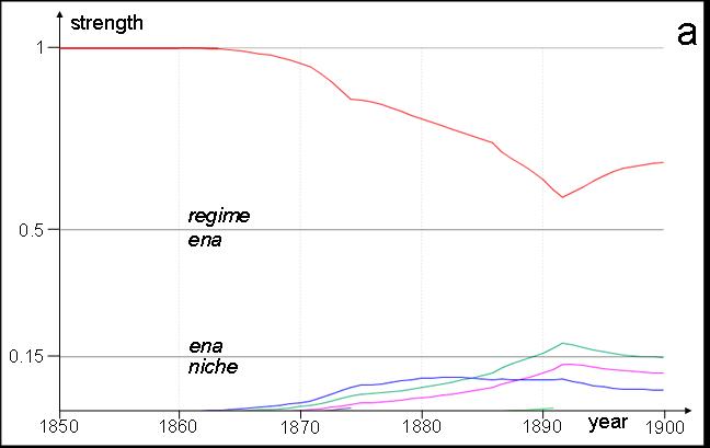
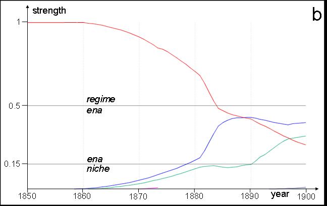
Figure 9. Normalised agent strengths for ten runs in example 3: The x-axis is time (years), the y-axis strength, with vertical sections differentiating niches (bottom), ENAs (middle) and regime (top); the red lines are the sailing ship agent, the blue lines the steam ship agent. This batch of ten runs shows steam ships becoming the new regime in nine runs, with steamships gaining strength and support more slowly in the last one. Note: there is symmetry in each run, due to there being only two agents.

Figure
Figure
Figure 10. Normalised agent strengths in example 4: the red line is the regime, all others are randomly generated niches. The x-axis is time (years), the y-axis strength, with vertical sections differentiating niches (bottom), ENAs (middle) and regime (top). In run (a) the regime absorbs two niches and fights competition from three others. In run (b) the regime absorbs only one niche, and later collapses, leaving no regime at the end of the run.

Reconfiguration pathway

5.10
This pathway showed the incumbent regime surviving in over 80% of the runs, through a combination of adaptation and absorbing the emerging niches and thereby changing its practices. In runs where the regime survived, it absorbed 2 or more niches approximately 80% of the time; this is a successful representation of the reconfiguration pathway, as we interpret the absorption of a niche as changing some parts of the regime — actors, techniques, technologies, etc., and our criteria included two or more absorptions. In a minority of runs, the regime survived primarily through adaptation of its practices, absorbing one niche or none at all — these could be classified as a transformation. In ~15% of the runs the regime collapsed, leaving 2 or more ENAs competing at the end of a run, with no new regime. In a few runs (ca. 3%), the regime failed and was displaced by an innovative niche; these runs are best classified as technological substitution. Figure 10 shows examples of a successful reconfiguration (a), and a regime collapse with no new regime (b).

5.11
The absorption mechanism was slightly changed in this pathway: rather than looking at angles (see 3.16), the regime attempts to absorb any niche that has higher values than it on both axes. In other words, the regime attempts to take up any practice that is more advanced than it in both organisation of production and mechanisation and division of labour. The distance limitation (Equation 2) is still used, indicating that the regime cannot take up practices too different from its current ones. The reason for this change was that the default absorption pattern led to an erratic trajectory as the regime absorbed niches in different directions, then changed its heading back towards the centre of the supporter 'cloud'. The change led to a more coherent trajectory, which better matched the historical example.

5.12
The regime does not necessarily absorb every new idea - some innovative niches remain in the system at the end of most runs. In approximately 60% of runs empowered niches emerged, gaining enough strength as to be a possible threat to the regime, but usually falling in power by the end of the run. It's worth noting that not all the niches were innovative — some emerged in areas of the practices space which the regime had left. These could be interpreted as traditional workshops, which had gone from the mainstream to being a specialised niche catering to a small number of people.

5.13
By contrast, in runs where the absorption mechanism was not used, the regime was not successful, and remained in power in only ~15% of runs, mainly due to its lingering strength — having more physical and institutional capacity than the new innovations. Only ~10% of runs without absorption showed a new regime at the end of the run, while most had competing ENAs without a new regime. Including the clustering mechanism increased the chance of a new regime appearing. The results of this example successfully demonstrate how when landscape signals are strong, the regime must change dramatically (represented here by absorbing niches and adaptation) or risk collapsing.

Technological substitution revisited

5.14
We summarise here results from separate work (Köhler and Schilperoord unpublished), in which we more thoroughly reproduced one historical example, in order to demonstrate that the model can be calibrated with real world data to reproduce a transition that has been identified in the literature. This was example 3, the historical transition from wooden sailing ships to iron and steel steam ships, two competing technologies for oceanic transport in the 19th century. In this case study, historical data on total registered tonnage and price change over time are used as exogenous data. Arguably, the cost reductions and technical change experienced in the shipbuilding industry were partly exogenous. The steam engine was important in all branches of industry, and shipping was able to benefit from developments in other areas, not just R&D in the shipbuilding industry.

5.15
An important new feature developed for modelling this case study is the investment decision of shipping companies, which modifies the agents' metabolism (see 3.20 - 3.21). The investment decision rule is specified as follows:

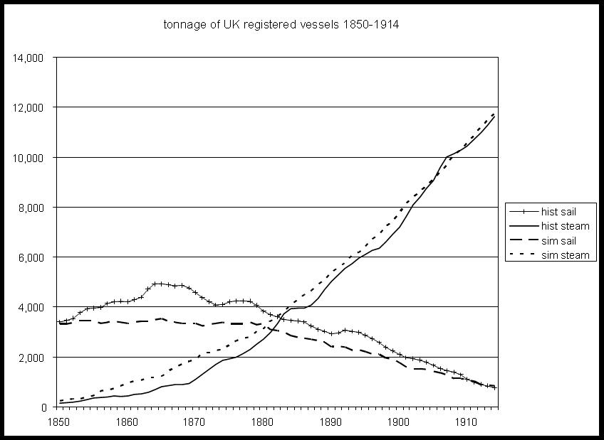
Ai(t+1) = (1 - delta) Ai(t) + delta Si(t) / Stotal(t) (15)

where A is attractiveness of agent i to the investor, S is the strength (as shares of registered tonnage of Great Britain in year t), and delta the fraction of resources to be reallocated.

5.16
The simulation is successful, reproducing the main features of the historical data, see Figure 11. Transition theory was useful, first, in leading us to think of landscape factors: there was an increase in demand due to general social/economic trends - European and US industrialisation and the economic development of the British Empire. This was partly driven by reduced shipping prices, but also part of the general trend of the time. And second, focusing on the existence of niches — the other critical causal factor, with a few customers willing to pay high prices for improved performance early on, leading to the take-off of steam ships.

Figure
Figure 11. Comparison of registered tonnage of sail and steam from historical data with model simulation results (Köhler and Schilperoord unpublished)

5.17
This case study also illustrates the need for a case-specific analysis. The sail-steam transition was heavily dependent on the relative costs of the two technologies, because both passenger and freight markets were highly competitive. Therefore, cost reducing improvements in technology were quickly adopted and were also quickly passed through to customers in the form of price reductions. This enabled both the expansion of the industry and also determined the form of technology adopted. Hence, the most important features in this case are differentiated markets, investment decisions, and relative costs and performance of the competing technologies.

Analysis

5.18
As the results above show, the model can capture the different transition pathways of Geels and Schot (2007), as well as the 'reproduction' pathway, in which there is no transition. Landscape changes and internal dynamics forced the regime to adapt or lose power and ultimately be replaced, portraying a transition. The technological substitution and de-alignment realignment pathways show transition through regime change, with the first showing an immediate replacement of the regime and the second a slower replacement, or repeated replacements until another stable regime emerges. The reconfiguration and transformation pathways show the regime surviving but changing, although the difference between these two pathways in the model is mainly a matter of interpretation.

5.19
However, capturing the different historical examples, even in the simplified forms presented here, was more difficult than reproducing the transition pathways. The calibration of model parameters and equations as detailed in section 4 still left results which didn't always match the historical example. In our ongoing work looking in more depth at different case studies, we use more quantitative data and sometimes a larger number of practices, in order to enable a more detailed and accurate history to be produced in the model, as is demonstrated in the detailed sail-to-steam example above. This example demonstrates that there is not necessarily a need for large quantities of data, but rather a wise choice of relevant data and additions to the model suffice for a detailed, accurate, example.

5.20
The conceptual model developed here can be used for a wide range of different empirical cases, and from it we implemented a generic model prototype, which is useful as a way of synthesising transition theory and as a base model which can be modified to suit a variety of examples. While details of each example require extensive changes to model parameters and rules, using the generic model as a starting point helps in highlighting the likely important parameters and dynamics in any specific example.

5.21
The present model makes it difficult to differentiate between consumer-led dynamics and other possibilities: in all runs landscape signals change the preferences of the supporters, ultimately changing the agents' strength, which relies on support. One change we have considered is having other forces affect supporter movement besides landscape signals. We experimented with two such rules: 'attractor' behaviour, in which the regime (and possibly other agents) draw supporters towards them, and with 'social' behaviour, in which supporters were less likely to move if they were in a high density part of the support canvas. Both of these behaviours made a transition less likely, as the supporter cloud around the regime was less likely to move. Further work on these types of rules is needed.

5.22
The technological substitution in the third example proved difficult to capture, despite a substitution by regime change being very easy to demonstrate in the generic model. We attribute this to insufficient feedbacks between the agent-based model and the systems dynamics model, specifically to the use of price as a practice axis. The more detailed analysis of this case study, using exogenous data on prices and linking the data to agent metabolism, proved more successful. The relative simplicity of this historical example, with two clearly distinct technologies and relevant data, made it tractable and relatively straightforward to model, and sheds light on the type of data needed for in depth case studies.

5.23
The behaviour rules chosen for the agents (hunt, predate, aggregate) were successful despite their simplicity, and resulted in complex, yet realistic dynamics. The notion of frontiers was also useful in limiting the possible movement of different agents. The only behaviour that yielded difficulty was the 'predate' behaviour of the ENAs. Conceptually, it makes sense for an ENA to copy some of the regime's practices in order to gain support and power from the regime. However, the results in the model sometimes showed unlikely behaviour or an illogical position with a regime and an ENA having nearly identical practices — arguably this represents clustering into one larger agent. The predate behaviour needs some modification.

5.24
The importance of the metabolism was evident in two things, and justifies our choice of more complex agents with internal dynamics. First, it helped the regime stay in power despite losing support, rather than collapsing as soon as its popularity decreased. Experimental runs with the metabolism switched off, where strength was determined only by support, were much more volatile, and power switched unreasonably fast. The dampening effect of the metabolism, whereby support determined long-term strength, but structure determined immediate strength gave the regime more power over the system, resulting in more realistic dynamics.

5.25
Second, agent structure, and specifically the time it takes a niche to build up its physical capacity, can change model dynamics. For example, in the de-alignment realignment pathway, runs without metabolism (see 5.6) showed trams taking over from horse-based transport quickly, because they had more support, with cars taking over later equally fast. The metabolism not only had a dampening effect here, but also provided more competition. As no niche had enough infrastructure (represented as PC) to take the place of the regime, the result was a better representation of the de-alignment/realignment scenario, with different agents prospering after the incumbent regime lost support.

* Conclusions and Discussion

6.1
We have reported on a modelling exercise in progress, which attempts to model different transition pathways, using concepts drawn from the literature on transitions (e.g., Rotmans et al. 2001), the taxonomy of Geels and Schot (2007) and the historical examples detailed therein, and our own conceptual framework (Haxeltine et al. 2008) that describes the mechanisms for agent interaction and the internal metabolism of agents. We have succeeded in modelling the different transitions pathways, with some degree of success at recreating the historical examples. The generic transitions model is valuable on the conceptual level, as a way of bringing together diverse aspects of transitions theory, and as a basis for developing each of the model applications to different empirical examples. We note that our ongoing work of more fully reproducing historical transitions, or making useful models of potential future transitions to sustainable development, requires more detailed case studies, adapting the model to each case. However, as noted above, the requirement is not necessarily for large quantities of data, but rather wise choices of good data and the right additions to the model can suffice for an accurate model.

6.2
The modelling has been co-evolving with our conceptual framework (Haxeltine et al. 2008), as both were developed in parallel. New ideas from the conceptual framework were tested in the model, and feedback from implementation shed light on conceptual ideas. It is a good exercise, if challenging, and we have learned much about the limitations of a conceptual model, as feedbacks conceived in narrative terms can turn out to be unexpectedly complex, or require much clarification, when put into equation form. It is important to remember that the field of transition theory is itself new and still maturing, and this modelling exercise will hopefully contribute to its further development.

6.3
In this modelling exercise we faced the challenge of achieving a model design that was both flexible enough to try various implementations, while also retaining a coherent overall model structure. While the model design is highly flexible, more changes were required than we originally envisaged in applying it to different examples, even highly simplified ones. Nonetheless, for specific case studies, our 'transition laboratory' interface allows the user to easily make a variety of run-time changes, such as turning on and off different mechanisms and choosing between different available landscape signals, as well as a variety of graphical displays useful for analysis (some of which have been shown in this paper). The resulting platform also leaves open options for future development, including: the possible addition of a more detailed economic model with features such as markets and learning curves; enhancing individual supporter decision making; specifying and resolving the actors which make up the regime and the niches (e.g., investors in shipping); and more.

6.4
In the historical examples presented here, it is known that a transition has occurred, and of what type. In case studies looking at potential future transitions to sustainability, we cannot say for certain if a transition will occur, and if so of which type. While this type of model is not intended to give predictions, it is nonetheless important that it yields realistic and meaningful results, which can be interpreted as possible future scenarios. Exercises such as this work can help in model calibration. The detailed historical example of sailing ships to steamships gives us an idea what to look for in future work.

6.5
One possible addition to the model being explored in the sustainability context is impacts. We intend to include sustainability indicators, and define the impacts of various practices on these indicators. The total impact of the system can then be calculated from the practices employed by the various agents defined in the model.

6.6
The next step in this research is to conduct empirically grounded modelling exercises using quantitative data sets where possible. We currently are developing four different case studies with different degrees of detail: besides the historical example detailed above, we are looking at a potential transition to sustainable housing and communities in the UK (Bergman et al. 2007; Bergman et al. 2008); a transition to sustainable water management in Spain; and a European transition to sustainable mobility (Whitmarsh and Nykvist 2008; Köhler et al. forthcoming). The last, which is our most advanced case study, follows our own research and other work into European transport systems and the hydrogen and fuel cell sectors, as well as stakeholder exercises (Whitmarsh and Wietschel 2008). Ideally, we would have stakeholder input throughout model development for relevant case studies, for validation of parameters and plausibility of results, as well as for honing clarity and usefulness of model output. In the longer term, we hope these models will prove useful in evaluating sustainability policy options.


* Notes

1 Methods and Tools for Integrated Sustainability Assessment (MATISSE). See: http://www.matisse-project.net

2 While this description is for regime change, we can expect a similar period of rapid change followed by stabilisation if a regime is transformed.

3 The transformation mechanism, in which an agent switches from one type to another, is not to be confused with the transformation transition pathway.


* References

BERGMAN, N, Whitmarsh, L, Köhler, J, Haxeltine, A and Schilperoord, M (2007). Assessing transitions to sustainable housing and communities in the UK. In Horner, M, Hardcastle, C, Price A and Bebbington J (Eds.) International Conference on Whole Life Urban Sustainability and its Assessment, Glasgow.

BERGMAN, N, Whitmarsh, L and Köhler, J (2008). Transition to sustainable development in the UK housing sector: from case study to model implementation. UEA: Tyndall Centre Working Paper.

DIEDEREN, P, van Meijl, H, Wolters, A, and Bijak, K (2003) 'Innovation Adoption in Agriculture: Innovators, Early Adopters and Laggards'. Cahiers d'Economie et Sociologie Rurales, 67, pp. 30-50.

DOSI G (1984) Technical Change and Industrial Transformation, London: Macmillan.

ELZEN, B, Geels, F W and Green, K (Eds.) (2004) System Innovation and the Transition to Sustainability: Theory, Evidence and Policy, Cheltenham, UK: Edward Elgar.

GEELS F W (2002) Understanding the dynamics of technological transitions: a co-evolutionary and socio-technical analysis, Enschede, The Netherlands: Twente University Press.

GEELS F W (2005a) 'Processes and patterns in transitions and system innovations: Refining the co-evolutionary multi-level perspective'. Technological Forecasting and Social Change, 72(6), pp. 681-696.

GEELS F W (2005b) Technological Transitions and System Innovation: A Coevolutionary and Socio-Technical Analysis, Cheltenham, UK: Edward Elgar.

GEELS, F W (2006a) 'The hygienic transition from cesspools to sewer systems (1840-1930): The dynamics of regime transformation'. Research Policy, 35(7), pp. 1069-1082.

GEELS, F W (2006b) 'Major system change through stepwise reconfiguration: A multi-level analysis of the transformation of American factory production (1850-1930)'. Technology in Society, 28(4), pp. 445-476.

GEELS F W and Schot J (2005) 'Taxonomy of transitions pathways in socio-technical systems' Presented at workshop by the ESRC Sustainable Technologies Program, May 12, 2005, London.

GEELS F W and Schot J (2007) 'Typology of sociotechnical transition pathways.' Research Policy, 36, pp. 399-417.

GIDDENS A (1984) The Constitution of Society, Cambridge: Polity Press.

HAXELTINE, A, Whitmarsh, L, Bergman N, Rotmans, J, Schilperoord, M and Köhler, J (2008) A Conceptual Framework for transition modelling. International Journal of Innovation and Sustainable Development 3(1-2), pp. 93-114.

HOOGMA R, Kemp, R, Schot, J and Truffer, B (2002) Experimenting for Sustainable Transport Experimenting for Sustainable Transport: the approach of strategic niche management, Routledge: London, New York.

KEMP, R and Rip, A (1998) "Technological Change". In Rayner, S and Malone, E L (Eds.), Human Choice and Climate Change, Volume 2 (pp. 327-399), Columbus, Ohio: Battelle Press.

KÖHLER, J, Grubb, M, Popp, D and Edenhofer, O (2006) 'The transition to endogenous technical change in climate-economy models: A technical overview to the Innovation Modeling Comparison Project'. Energy Journal, pp. 17-55.

KÖHLER, J, Whitmarsh, L, Nykvist, B, Schilperoord, M, Bergman, N and Haxeltine, A (forthcoming). Mobility ISA Case Study Report. Submitted to Technological Forecasting & Social Change.

KÖHLER, J and Schilperoord, M (unpublished). Report on a historical calibration case study for the MATISSE WP9 transitions model: A new perspective on the transition from Sail to Steam in Ocean Shipping. MATISSE Final Deliverable Report.

LAVER M (2005) 'Policy and the dynamics of political competition'. American Political Science Review, 99(2), pp. 263-281.

LOORBACH D and Rotmans J (2006) "Managing transitions for sustainable development". In Olshoorn X and Wieczorek A J (Eds.) Understanding Industrial Transformation: views from different disciplines Dordrecht: Springer.

NOBLE T (2000) Social Theory and Social Change, Basingstoke: Macmillan.

ROGERS, E M (1995) Diffusion of Innovations (4th ed.). New York: Simon and Schuster.

ROTMANS, J, Kemp, R and van Asselt, M (2001) 'More evolution than revolution: transition management in public foreign policy'. Foresight 3(1), pp. 15-31.

ROTMANS J (2005). Societal innovation: Between dream and reality lies complexity, Rotterdam: Inaugural Address, Erasmus Research Institute of Management.

SCHWOON M (2005). Simulating The Adoption of Fuel Cell Vehicles. Working Paper, FNU-59 Research unit Sustainability and Global Change, Hamburg University.

SMITH, A, Stirling, A and Berkhout, F (2005) 'The governance of sustainable socio-technical transitions'. Research Policy, 34(10), pp. 1491-1510.

TURNPENNY, J, Weaver, P M, Rotmans, J, Haxeltine, A and Jordan, A (2007) 'Methods and Tools for Integrated Sustainability Assessment'. Chapter 9 in George C and Kirkpatrick C (Eds.) Impact Assessment for a New Europe and Beyond, Cheltenham, UK: Edward Elgar.

WEAVER P M (2005) 'Integrated Sustainability Assessment: toward a new paradigm'. In Blaas W (Ed.) Der Öffentliche Sektor — Forschungsmemoranden: Multi-level Governance for Sustainability. 31(1-2), pp. 47-53.

WHITMARSH L and Nykvist B (2008). Integrated sustainability assessment of mobility transitions: Simulating stakeholders' visions of and pathways to sustainable land-based mobility. International Journal of Innovation and Sustainable Development. 3(1-2), pp. 115-127.

WHITMARSH L and Wietschel M. (2008). Sustainable transport visions: What role for hydrogen and fuel cell vehicle technologies? Energy and Environment 19(2), pp. 207-226.

----

ButtonReturn to Contents of this issue

© Copyright Journal of Artificial Societies and Social Simulation, [2008]