Ayse Mumcu and Ismail Saglam (2008)

Marriage Formation/Dissolution and Marital Distribution in a Two-Period Economic Model of Matching with Cooperative Bargaining

Journal of Artificial Societies and Social Simulation vol. 11, no. 4 3
<https://www.jasss.org/11/4/3.html>

For information about citing this article, click here

Received: 13-Sep-2007    Accepted: 08-Jun-2008    Published: 31-Oct-2008

Abstract

We study the problem of marriage formation and marital distribution in a two-period model of matching, extending the matching with bargaining framework of Crawford and Rochford (1986). We run simulations to find the effects of alimony rate and legal cost of divorce parameters on the payoffs and marital status in the society.

Keywords:

Matching, Bargaining, Marriage, Divorce, Marital Distribution

Introduction

1.1

Being unmarried, married or divorced are decisions faced by every human being during his/her lifetime with far-reaching economic implications both for individuals and for the society as a whole. While in most societies, these decisions are taken by individuals, hence determined by individual preferences, they are also significantly shaped by social norms that draw the boundaries of the pool of eligible mates, civil laws that govern marital dissolution, and economic environments that frame marriage and divorce possibilities.

1.2

In the last hundred years, the divorce rates have experienced a sharp increase.^[1] The positive welfare effects of divorce through facilitating the termination of malfunctioning marriages (e.g. marriages involving domestic violence and child abuse) have, on average, been outweighed by post-separation costs especially borne by women and children.^[2] The rise in the divorce rates has consequently attracted the attention of researchers in understanding and modelling the formation of marriages and marital dissolution, and increased the awareness of policy makers towards taking measures to enhance the stability of marriages as well as to alleviate the post-separation costs.

1.3

An early strand of literature that followed the pioneering work of Samuelson (1956) and Becker (1974, Becker 1981) on common preference models of family, omitted the problem of formation of marriages and only studied strategic considerations within the family. Manser and Brown (1980) and McElroy and Horney (1981) modelled family demands as an outcome of a bargaining solution where threat points of agents were taken to be exogenously determined payoffs from divorce. Although these models on marriage commonly missed one important element, namely, the matching market, the implications of its absence was neither long unnoticed nor underestimated. Indeed, Becker (1981) himself emphasized the importance of matching market as a determinant of wealth distribution between men and women. As he pointed out, wealth distribution within marriage not only depends on partners' respective contributions to marriage but also on alternative matches available to each partner in marriage market. The other direction of the interaction between the formation of marriages and marital (wealth) distribution was later noticed by Lundberg and Pollak (1993), who argued that policies that transfer income from husbands or wives affect not only the marital distribution of surplus within existing marriages but also the number of equilibrium matchings in subsequent marriage markets.

1.4

Recently, there have been studies that model the relationship between marital choice and marital distribution in a search-theoretic framework. Individuals, in these studies, draw from a distribution of mates in the marriage market, and decide whether to marry or make further searches. Marriage is desirable since couples pool their income hence obtain a greater level of consumption. Moreover, partners learn about the quality of match over time and it is the arrival of new information that triggers divorce. Couple's decision to end marriage also depends on the prospect of remarriage. This is introduced into the models by assuming that probability of remarriage is increasing in the number of singles in the market. The equilibrium marriage and divorce rates, and consumption allocations are all calculated under rational expectations.

1.5

In the described search-theoretic framework, Bougheas and Georgellis (1999) examined the effect of divorce costs on both marriage formation and dissolution. Aiyagari et al (2000) constructed an overlapping generations search model of marriage and divorce, and examined the effects of antipoverty policies (child support and welfare) on decisions to marry, divorce and invest on children. Greenwood et al (2003) extended the Aiyagari et al (2000) by endogenizing the family size. Chiappori and Weiss (2006) studied, in a search-theoretic general equilibrium model of marriage, the determination of divorce transfers.

1.6

Another strand of literature that combines evolutionary psychology and cognitive sciences studies mate choice using agent-based computational models. These models specify how individuals meet, learn over time, and decide about potential partners. The simulation results can be tested against the observed subjective behaviour, both at an individual and population level (Miller and Todd 1998, Simao and Todd 2002, Simao and Todd 2003 and Todd et al 2007 to name a few.)

1.7

In this paper, we deal with the said problem of marriage formation and marital distribution in a model of 'matching', differing from and partially improving over both computational mate choice models and search-theoretic models. Unlike in computational mate choice models, individuals in our model integrate wealth characteristics of each prospective mate with the other observed physical and psychological traits (that we simply model in this paper by emotional utilities) to obtain assessments of overall attractiveness of potential mates. Moreover, we also consider the issue of marital distribution, which is entirely missing in the agent-based mate choice literature, not only as a separate issue by itself but also taking into account its calculated implications on the marital decisions of agents. Differing from both search-theoretic models and computational mate choice models, agents in our model consider the whole set of mates to be feasible, completely know the values of all prospective mates, and thus they perfectly decide to whom to propose for marriage.^[3]  Consequently, reaching to a stable matching is always warranted. In search models, where potential couples meet sequentially at finite rates and the qualities of potential matches are unknown, individuals draw from a commonly known distribution of mates in the marriage market and look for a new mate until the costs of an additional search outweigh the benefits that could be gained by leaving the sampled candidate at hand. In computational mate choice models, individuals search until they find a prospect whose attractiveness value exceeds a reasonable aspiration level. Clearly, the matching processes characterized by sequential search decisions under incomplete information about the values of prospective mates lead to the possibility of dynamically unstable marriages or courtships in both search models and mate choice models.

1.8

In this paper, individuals' decisions to be unmarried, married, divorced and remarried along with wealth distribution within the marriage are determined and analyzed in a two-period matching model through a recursive bargaining process, which is borrowed from Crawford and Rochford (1986) (hereafter CR). We consider a small economy inhabited by two men and two women living for two periods.^[4]  Each individual is born with an endowment (not necessarily identical) and they have mate-specific emotional utilities reflecting their affection to each possible match. A match between a man and a woman produces a surplus that is assumed to be linearly increasing in the total endowment of the couple. If an individual chooses to stay single then he/she produces a surplus combining his/her endowment with a single productivity parameter. Marital distribution is determined via Nash bargaining with the threat point of an individual being given by his/her bargaining payoff from an alternative mate.^[5] 

1.9

Initially no agent is married. At the beginning of each period marriage market opens, allowing agents to change their marital status. In each period, agents reach to men-optimal stable matching^[6]  and obtain the implied bargaining payoffs using the 'matching with bargaining equilibrium' of CR. The recursive procedure proposed by CR calculates the disagreement points for a given pair of agents as the bargaining equilibrium payoffs that they would receive in a reduced market obtained by setting the match between the pair in consideration unproductive and letting the match opportunities of all other agents unchanged.^[7]

1.10

We assume that agents can divorce at the end of the first period unilaterally, and in such an event separating partners incur a legal divorce cost and person-specific emotional distress. Moreover, man is obliged to pay to woman a fraction of his period-one marriage surplus as an alimony.^[8]  Beginning-of-second period endowment of each individual is then determined by his/her period-one bargaining payoff net of all types of divorce costs (if any).

1.11

Due to the recursive nature of the bargaining equilibrium, the closed-form solution of the problem cannot be obtained. Thus to make comparative statics, we simulate the model for an artificial economy. In response to changes in the alimony rate and the legal cost of divorce, we examine the changes in the payoffs of men, women, and the whole society as well as changes in the frequencies of being i) single in both periods, ii) married only in the first period, iii) married only in the second period, iv) married with distinct mates in the two periods, v) married with the same mate in both periods.

1.12

The organization of the paper is as follows: Section 2 introduces the model. Section 3 presents our simulation results and relates them to the existing theoretical and empirical literature. Section 4 concludes.

Model

2.1

We consider a society with two men m₁,m₂ and two women w₁,w₂ living for two periods indexed by t=1,2. The set of men and women are denoted by M and W, respectively. The set of all possible feasible assignments of women to men are denoted by M = { μ : W → M | μ is one-to-one}.

2.2

The endowment of agent i (men or women) at the beginning of period t is e_i(t), a nonnegative real. Agent i is born with e_i(1); however e_i(2) which we call an interim endowment is acquired from the share of the total marriage surplus at the end of the first period. The emotional utility of agent i derived from a match with agent j in period t is u_i(j,t), a real. The emotional utility of agent i from being single is normalized to zero, i.e. u_i(i,t)=0.

2.3

The marriage market in period t is defined as the complete list of endowments and all utility possibilities, and denoted by Ω_t.

2.4

We assume that the match between man i and woman j converts total endowments into total utility E_ij(t) to be shared (bargained over) through a linear production technology^[9], i.e., 

(1)   E_ij(t) = f_ij[e_i(t)+e_j(t)] 

where the linear productivity parameters are nonegative real numbers and satisfy f_ij = f_ji.

2.5

The disagreement point from a match between man i and woman j is (d_i(j,Ω_t),d_j(i,Ω_t)). In our one-to-one matching market with transferrable utility, bargaining problems are solved by applying Nash (1950) solution, which yields to agents equal shares of gains from cooperation.^[10]  Thus, the payoff to agent i when matched with j is

(2)    π_i(j;Ω_t)=max{b_ie_i(t),u_i(j,t)+min{E_ij(t),(1/2)[E_ij(t)+d_i(j,Ω_t)-d_j(i,Ω_t)]}}

where a nonnegative real number b_i denotes the productivity parameter of the linear technology that converts agent i's endowment into end-of-period utility when he/she is single. Equation (2) ensures that all the surplus from a marriage is distributed and each agent gets when married at least as great as when he/she is single.

2.6

Agent i who is matched in period 1 incurs legal divorce cost c, and an emotional distress c_i^u at the end of the period if he/she divorces from his/her mate.^[11]  In addition, in the event of divorce, man is obliged to pay to woman a fraction, a, of his end-of-period 1 marriage surplus (in endowment terms) as an alimony.

Thus, the period 2 endowment of man i who divorces from woman j at the end of period 1 is 

(3)    e_i(2)= (1-a)[π_i(j;Ω₁) - u_i(j,1)]- c

and the period 2 endowment of woman j who divorces from man i at the end of period 1 is^[12]  

(4)    e_j(2)=π_j(i;Ω₁) - u_j(i,1) +a[π_i(j;Ω₁) - u_i(j,1)]- c. 

2.7

The period 2 emotional utility of agent i who divorces from agent j at the end of period 1 and considers to be matched with agent k is 

(5)    u_i(k,2)=u_i(k,1)-c_i^u. 

Agent i feels no emotional distress if he/she does not divorce from his/her mate.

2.8

Now, we are ready to define an allocation and bargaining equilibrium in the marriage market. Here, we will assume that the marriage market Ω_t as well as the list ({f_i,j}_(i,j) є _M×W, {c^u_i,b_i}_i є_M∪W, a, c) are common knowledge.^[13] 

2.9

An allocation in the marriage market  Ω_t consists of a payoff vector x(.,t) and an assignment of agents μ(.,t), where μ(m,t) є {m} ∪ W for each m є M and μ(w,t) є {w} ∪ M for each w є W.

2.10

Borrowing from CR, we define a bargaining equilibrium for Ω_t as an assignment/payoff pair (μ(.,t),x(.,t)) such that^[14]  

(6)    x(m,t)=π_m(μ(m,t);Ω_t) for all m є M, and  x(w,t)=π_w(μ(w,t);Ω_t) for all w є W,

(7)  there do not exist agents m є M and w є W such that π_m(w;Ω_t)>x(m,t) and π_w(m;Ω_t)>x(w,t). 

2.11

Condition (6) requires that agents matched under μ(,.t) obtain payoffs determined by the bargaining solution in (2). Condition (7) simply requires that no pair of agents have strict incentives to block the matching μ(,.t). Together with the bargaining solution in (2), which checks the incentive of each agent to individually block a given matching, condition (7) defines the stability notion in the usual way.

2.12

To compute the bargaining equilibrium in the marriage market, we will slightly modify recursive procedure by CR to allow for situations in which agents have emotional utilities. Once agents' preferences over possible matches are fixed at any stage of this recursive procedure, one can apply Gale and Shapley's (1962) 'Deferred Acceptance Algorithm' (DAA) to find a stable matching that is always known to exist (under some mild assumptions on preferences, such as completeness and transitivity, which are trivially satisfied in our model).^[15]  Of the two versions of the DAA, we employ the DAA with men proposing and obtain the men-optimal stable matching in each step of the recursive procedure. Below, we first present DAA with men proposing.

2.13

DAA with Men Proposing: In the DAA with men proposing, initially nobody is engaged (assigned) or rejected. In each iteration, an unassigned man proposes to the first acceptable woman on his list that he has not proposed to yet. A woman who receives a proposal that she prefers to her current assignment accepts it and rejects her current assignment. The algorithm stops after any step in which every man has either been rejected by every acceptable women on his list or is engaged to an acceptable woman. (By interchanging the names of men and women, the DAA with men proposing simply changes to the DAA with women proposing.)

2.14

The modified CR procedure for finding the bargaining equilibrium in the marriage market in a given period is simply described below. (A lengthier version of the procedure is also available at the Appendix.)

2.15

Possible marriages in a society, involving two men and two women, are denoted by the pairs p₁=(m₁,w₁), p₂=(m₁,w₂), p₃=(m₂,w₁), p₄=(m₂,w₂). We define the set P={p₁,p₂,p₃,p₄}. For any subset F of P, let Ω_t[F] be the restriction of Ω_t on F. Clearly, Ω_t[P]=Ω_t.

2.16

Below, we introduce a recursive procedure, called CR(F;Ω_t[F]), which will compute the period-t equilibrium payoffs for each marriage in F using the endowment and utility information in Ω_t[F]. Apparently, CR(P;Ω_t) will compute the period-t equilibrium in our described marriage market.

Procedure CR(F,Ω_t[F]):

Step 1: Pick any match p=(m,w) є F. We construct the reduced market Ω'_t[F] from Ω_t[F] by setting the match p as unproductive, i.e. 

(8)    π_m(w;Ω'_t[F])=b_me_m(t) and  π_w(m;Ω'_t[F])=b_we_w(t) 

and letting Ω'_t[F]=Ω_t[F] for all pairs in F\{p}.

Step 2: Using payoffs for p assumed in Step 1 and computed equilibrium payoffs CR(F\{p}_,Ω_t[F\{p}]) for the marriages in F\{p}, compute the men-optimal stable matching and the implied payoff structure x'(.,t) for Ω'_t[F].^[16]  

Step 3: Set the disagreement payoffs of spouses in p to their payoffs calculated in Step 2, i.e., 

(9)    d_m(w;Ω_t[F])=x'(m,t)-u_m(w,t)  and  d_w(m;Ω_t[F])=x'(w,t)-u_w(m,t).

By conditions (8) and (9), the threat points of the pair (m,w) in the market Ω_t[F] are taken as their equilibrium payoffs in the reduced market Ω'_t[F] (net of the emotional utilities from their current mates), where they are forced to remain single while all other agents can still exploit all of their opportunities.

Step 4: Compute equilibrium payoffs of p using the Marriage rule.

Marriage Rule: For the agents forming a given pair, calculate the bargaining payoffs using equation (2). Divorce the agents if and only if at least one of the agents is not worse off by remaining single. In that case, assign to both agents in the pair the payoffs from being single.

Step 5: Repeat steps 1-4 for each match p in F.

Step 6: Using payoffs for each p in F as calculated in Step 4, compute the men-optimal stable matching and the implied payoffs for each match in F.

2.17

Having described our model and our marital equilibrium procedure, we can now summarize the functioning of our simple marriage economy involving 2 men and 2 women. In period 1, a marriage market opens and all agents participate. The stable matchings are determined via Gale and Shapley's men-proposing DAA. However, one gender's rankings of the other is endogenously determined within the model. The recursive CR procedure computes stable matchings for an economy through finding the implied preferences of the agents based on their bargaining share from the potential marital surplus. The bargaining share of an agent depends on his/her threat point (that is his/her share from an alternative mate), which in turn depends on the order in which a man proposes to a woman. For every individual, starting with a market containing an arbitrary couple, the threat point is calculated recursively as his/her equilibrium payoff to a stable match (which may include the prospect of being single as well) that will be obtained as the market includes more participants, of both gender, for all combinations of new arrivals. In the second period, all marriages are artificially dissolved and the CR procedure is applied to the new economy with the updated endowment vector. Those individuals who are matched with their first period mates are considered to be married to the same partner for their lifetime. Others either switch mates or change their marital status from being married to single or vice versa.

Simulation Results

3.1

Using the GAUSS (version 6.0) we simulated the model for an artificial economy involving two men and two women. (The program codes and the simulated data are available from the authors upon request.) The parameter values are listed in Table 1. The numbers in curly brackets are the common set of values that the parameters just above them take.

Table 1: Parameter values
Tastes	um1(w1,1), um1(w2,1), um2(w1,1), um2(w2,1)  { 0.28, 0.59, 0.94, 1.31, 1.72, 2.15, 2.62}
	uw1(m1,1), uw1(m2,1), uw2(m1,1), uw2(m2,1)   {0.24, 0.50, 0.77, 1.09, 1.44, 1.86, 2.35}
	cum1, cum2, cuw1, cuw2  {0.39, 0.49, 0.60, 0.70, 0.81, 0.9, 1.02}
Endowments	em1(1), em2(1), ew1(1), ew2(1)  {1.04, 2.64, 4.80, 7.51, 10.78, 14.60, 18.98}
Productivity parameters	fm1w1, fm1w2, fm2w1, fm2w2  {0.50, 0.75, 1.00, 1.25, 1.50, 1.75, 2.00}
	bm1, bm2, bw1, bw2  {0.44, 0.66, 0.87, 1.09, 1.30, 1.52, 1.73}
Policy variables	a, c  {0.13, 0.25, 0.38, 0.50, 0.63, 0.75, 0.88}

3.2

The model involves 26 parameters each of which admits 7 distinct values. Out of 7²⁶ possible simulations, we have chosen a total of 2401 to run due to CPU constraints of our computing machine. The data set which can be reported in a spreadsheet involving 2401 data rows for 26 parameter columns has the following pattern: For any parameter x which takes seven ascending values in {x₁,x₂,...,x₇}, there exists a frequency value k_x such that in data column for parameter x, the first k_x rows contain x₁, the next k_x rows contain x₂, ..., the seventh k_x rows contain x₇. The first 7k_x rows of data column for x repeat themselves 2401/(7k_x) times as a whole. The below table reports the frequency value k_x for each model parameter x. (Parameters in the first row have the frequency value 343, while those in the last row have the frequency value 1.)

Table 2: Frequency values of parameters in datasheet
343	um1(w1,1),   uw2(m2,1),   cum1,   em1(1),    fm1w1,   bm1,   c
49	um1(w2,1),   uw1(m2,1),   cum2,   em2(1),   fm1w2,   bm2
7	um2(w1,1),   uw2(m1,1),   cuw1,   ew1(1),   fm2w1,   bw1
1	um2(w2,1),   uw1(m1,1),   cuw2,   ew2(1),   fm2w2,   bw2,   a

3.3

The single and couple productivity parameters take artificial values which are above, below, and equal to, 'one' to allow for all distinct cases of constant returns to scale. Couple productivity parameters take, on average, higher values than single productivity parameters, in line with the recent empirical finding of Zagorsky (2005).^[17]  The rest of the model parameters are artificially chosen to yield a set of equilibria involving diverse marital decisions.

For the model parameters a and c we shall below analyze the variation in the average values (using 343 observations for each value of these two input variables) of the output variables in the list ( x(M,2),  x(W,2),  x(MW,2),  M(ss),  M(sm),  M(ms),  M(mm-c),  M(mm-n),  W(ss),  W(sm),  W(ms),  W(mm-c),  W(mm-n),  MW(ss),  MW(sm),  MW(ms),  MW(mm-c),  MW(mm-n) ) . Here, x(M,2), x(W,2), and x(MW,2) are respectively the total payoffs of men, women, and the whole society, in the second period, while for any group Z in {M,W,MW} (men, women, society) the output variables Z(ss),Z(sm), Z(ms),Z(mm-c),Z(mm-n) respectively denote the frequencies of  'being single in both periods, married only in the second period, married only in the first period, married with distinct mates in the two periods, married with the same mate in both periods'. We should note that M(mm-n) and W(mm-n), and hence MW(mm-n), always take the same values.

3.4

The marital status of the population for the simulated sample is exhibited in Table 3. The percentage of divorced couples, MW(ms)+MW(mm-c), is 23.28%, while 27% of these couples remarry after divorce. Calculating MW(mm-n)/ [MW(mm-n)+MW(mm-c)] shows that 89% of the marriages are stable. Moreover, as should be evident from MW(sm)/[MW(ss)+MW(sm)], approximately 10% out of the first-period singles get married in period two.^[18]

Table 3: Marital status (percentage distribution)
Male	M(ss) 23.41	M(sm) 3.00	M(ms) 17.45	M(mm-c) 5.83	M(mm-n) 50.31
Female	W(ss) 24.32	W(sm) 2.08	W(ms) 16.53	W(mm-c) 6.75	W(mm-n) 50.31
Society	MW(ss) 23.87	MW(sm) 2.54	MW(ms) 16.99	MW(mm-c) 6.29	MW(mm-n) 50.31

3.5

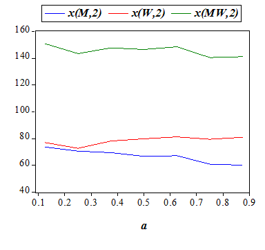
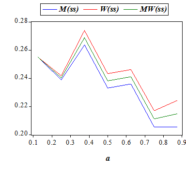
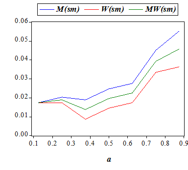
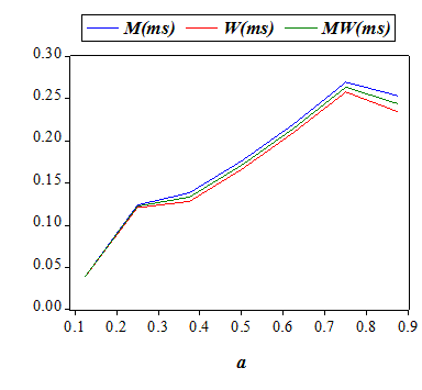
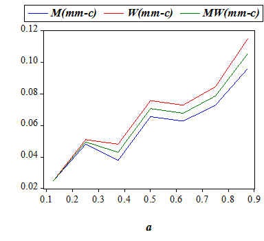
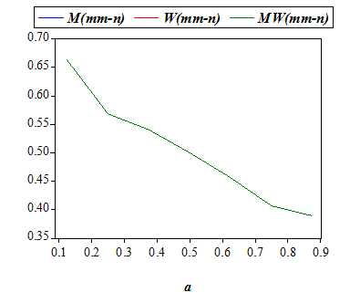
Figures 1-6 exhibit comparative static results with respect to the alimony rate. In Figure 1, the women's payoff is increasing and men's payoff is decreasing, while the overall payoff is slightly decreasing. In Figure 2, the frequency of being single in both periods declines for both genders except for a pike around 0.35. In contrast, the frequency of being married only in the second period is rising in Figure 3 for both men and women except for a slight dip around 0.4. The frequencies of being married only in the first period are escalating in Figure 4 up to 0.75. However, Figure 5 shows that the frequencies of being married to different partners in the two periods are fluctuating with a steep upward trend. The sum of the two, which is the frequency of divorce, is also increasing. Finally, the frequency of being married to the same partner in both periods falls for each gender, as plotted in Figure 6.

Figure 1	Figure 2

Figure 3	Figure 4

Figure 5	Figure 6

3.6

The above results are also summarized in Table 4.

Table 4: Summary of the effects of an increase in alimony rate (a)
(+=  increasing;   - = decreasing;    ~ = fluctuations)
	Men	Women	Society
Payoffs	-	+	- (slightly)
Frequencies
Single-Single	- with ~	- with ~	- with ~
Single-Married	+ with ~	+ with ~	+ with ~
Married-Single	+ with ~	+ with ~	+ with ~
Married-Married (Distinct Mates)	+ with ~	+ with ~	+ with ~
Married-Married (Same Mate)	-	-	-

3.7

The intuition underlying the above observations is that a higher alimony rate implies higher post-divorce financial wealth for a woman married during the first period. A wealthier divorced woman may now be able to seek a more profitable marriage with a wealthier man who did not find that particular woman admissible at the beginning of the first period.^[19]  Or it may even be the case that a divorced woman with sufficiently high earnings from divorce proceedings may no longer find any man (equivalently any marriage) desirable (profitable) in the second period and may choose to become single.^[20]   The divorce decisions of married women clearly imply a change in the marital status of their initial spouses as well as their prospective spouses, if any.

3.8

One can also interpret the parameter a as the child support benefit paid to the custodian partner, which happens to be women in our model. Then, our model predicts that child support has positive effects both on the rate of marriage and on the rate of divorce. While the former is in line with, the latter contrasts with, Aiyagari et al (2000). However, in the same context, Greenwood et al (2003) finds small effects of child support on the equilibrium number of marriages.

Figure 7	Figure 8

Figure 9	Figure 10

Figure 11	Figure 12

3.9

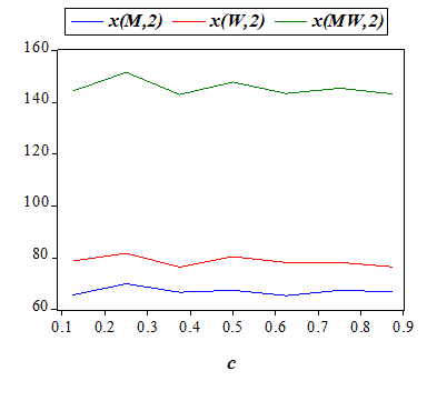
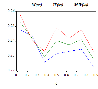
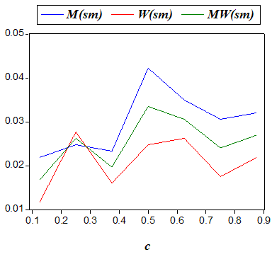
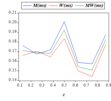
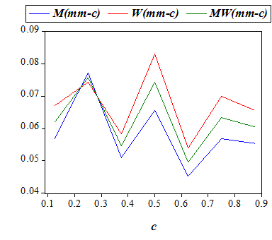
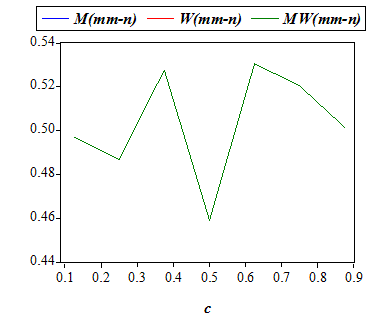
The effects of legal cost of divorce on the model outcomes are presented in Figures 7-12. Since the cost parameter c takes values relatively low with respect to the magnitudes of endowments, its direct effect on the payoffs of separating couples is already expected to be small. The almost horizontal behavior of payoffs in Figure 7 reveals that the indirect effects of c, due to changed marriage opportunities by the changed endowment structure, must also have been negligibly small. The divorce frequencies fluctuate on a relatively wider band with respect to the changes in the legal cost of divorce and reach maxima around 0.5 in Figure 10, while at this very level, the frequencies of continuing marriages attain their minimum in Figure 12. Figures 8, 9, and 11 respectively show that the frequencies of remaining always single, getting married after the first period, and changing the spouse in the second period are all fluctuating in narrow bands, for both men and women, in response to changes in the legal cost of divorce.

3.10

The above results are also summarized in Table 5.

Table 5: Summary of the effects of an increase in cost of divorce (a)
(~ = fluctuations)
	Men	Women	Society
Payoffs	~ (small)	~ (small)	~ (small)
Frequencies
Single-Single	~ (small)	~ (small)	~ (small)
Single-Married	~ (small)	~ (small)	~ (small)
Married-Single	~ (large)	~ (large)	~ (large)
Married-Married (Distinct Mates)	~ (small)	~ (small)	~ (small)
Married-Married (Same Mate)	~ (large)	~ (large)	~ (large)

On the effect of divorce cost on the marital decisions, Becker (1976) argued that when divorce becomes easier, the number of people who are legally married may actually increase, which is only partially supported by our findings (Figures 9 and 11). However, empirical studies examining the impact of changing divorce legislation on marital status are also conflicting.^[21] While Peters (1986, 1992) find no significant impact of changing divorce laws on divorce rates, Allen (1992) and Friedberg (1998) refute her finding. Recently, Wolfers (2006) reports that the divorce rate rose sharply following the adoption of unilateral divorce laws, but this rise was reversed within about a decade hence the long-run effects are ambiguous. Brien et al (2006) finds that decrease in divorce cost leads to a slight increase in the rate of marriage.

3.11

We should note that the diverse range of empirical results listed above are in fact not invalidated by our simulations in Figures 7-12. The reason why our model predicts fluctuations rather than monotone changes in the marital decisions of agents with regard to a rise in the legal cost of divorce is the heterogeneity of wealth within the society. A change in the legal cost of divorce redefines the relative wealth levels of the married, divorced as well as single agents. A rise in the divorce cost obviously reduces the relative bargaining power (wealth) of a divorced agent in seeking marriage, but whether this would consequently lead to an increase or decrease in the admissibility/desirability of a divorced agent from the viewpoint of agents from the opposite gender entirely depends on the distribution of the accumulated wealth in the society at the end of the first period. With a higher level of divorce cost, a divorced agent whose post-divorce wealth has been reduced to a moderate level may suddenly become a prospective spouse that is financially desirable in the second period at least for some divorced or single agents with moderate wealth, whereas an agent who has been divorced and been rendered extremely poor by the raised costs of separation may indeed become wholly undesirable as a spouse and hence be forced to become single in the second period.^[22] 

Conclusion

4.1

In this paper, we have introduced a two-period optimization model to study the issues of marriage formation and marital dissolution using the recursive solution procedure proposed by Crawford and Rochford (1986) for the problem of matching under cooperative bargaining.

4.2

We have simulated our model for an artificial set of parameters to examine the effects of the rates of alimony and legal cost of divorce on the marital status of agents in the society as well as on their marital payoffs. Our findings show that a higher rate of alimony to women is increasing not only the post-divorce payoffs of women (at the expense of a reduction in men's post-divorce payoffs) but also the divorce rate, albeit with some minor fluctuations. Moreover, we show that even small changes in the divorce cost, which yield hardly visible effects on the post-divorce distribution of wealth in the society, may lead to rather significant fluctuations in the marital status of both men and women. We believe that the observed unstable dependence between the marital decisions and the cost of divorce, which we argue is entirely generated by the heterogeneity of the optimizing agents with regard to their initial endowments, may indeed help to explain a diverse range of conflicting empirical results in the existing literature of marriage.

4.3

Differing from the existing search-theoretic literature that has emphasized the random nature of meeting a potential mate, our paper is indeed a first attempt to model the formation of marriage and marital dissolution by the use of optimization in a completely deterministic matching framework. We should admit that the pool of feasible mates for each individual may in reality expand over time by controlled as well as uncontrolled entrances of new candidates, i.e. the formation of mate pools is to some extent random in nature. However, it is hardly acceptable that individuals determine their prospective partners by random draws from any given pool of feasible mates. Instead, individuals make pairwise comparisons within the pool and form (usually short) preference lists, according to which they make sequential proposals for marriage. The interaction of the separate decisions of individuals on the opposite sides of the marriage market then determines the equilibrium matches. In this respect, while both search-theoretic models and the matching model we develop here have their own uses and strengths, a more complete framework of a marriage market can, of course, integrate the two, taking also into consideration the potential benefits of non-cooperative versus cooperative bargaining in simultaneously resolving the marital distribution and determining the marital choice.^[23] 

Appendix

A.1

This Appendix contains the procedure of finding the bargaining equilibrium in a given period.

Step 1:  Pick a permutation {p_i,p_j,p_k,p_l} of the pairs p₁=(m₁,w₁), p₂=(m₁,w₂), p₃=(m₂,w₁), p₄=(m₂,w₂).

Step 2:  For the agents forming the pair p_l, set the disagreement points equal to the payoffs from being single and calculate the bargaining payoffs using the Marriage Rule. Next, for the agents entering both p_k and p_l set the disagreement points to their calculated bargaining payoffs in the pair p_l, and for the remaining agents in p_k set the disagreement points to the payoffs from being single. Then, as the outcome of this step, determine the marital status and bargaining payoffs of the pair p_k using the Marriage Rule.

Step 3:  Repeat step 2 by interchanging the roles of p_l and p_k, and obtain the marital status and bargaining payoffs of the pair p_l.

Step 4:  Using the bargaining allocation obtained for p_k and p_l in steps 2 and 3, respectively, find the men-optimal stable matching for the agents in p_k U p_l.

Step 5:  For the agents in p_j, set the disagreement points to the bargaining payoffs obtained under the stable matching calculated in step 4 if these agents are also in p_k or p_l, and otherwise set them to the payoffs from being single. Then, find the marital status and payoffs for the pair p_j using the Marriage Rule.

Step 6:  Repeat steps 2-5 consecutively for the permutations (p_i,p_k,p_j,p_l) and (p_i,p_l,p_j,p_k), and obtain the marital status and payoffs of the pairs p_k and p_l, respectively.

Step 7:  Let the pair p_i be unproductive and the agents in p_i have their payoffs from being single.

Step 8:  Using the marital status and payoffs assumed or calculated for p_i, p_j, p_k, and p_l in steps 2-7, find the men-optimal stable matching and the implied payoffs.

Step 9:  For the agents in p_i, set the disagreement points to their bargaining payoffs calculated in step 8. Next, find the marital status and bargaining payoffs of the pair p_i using the Marriage Rule.

Step 10:  Repeat steps 2-9 consecutively for the permutations (p_j,p_i,p_k,p_l), (p_k,p_i,p_j,p_l), (p_l,p_i,p_j,p_k), and obtain the marital status and bargaining payoffs for the pairs p_j, p_k, and p_l, respectively. Step 11:  Using the marital status and bargaining payoffs calculated for the pairs p_i, p_j,p_k, and p_l, determine the men-optimal stable matching (hence the bargaining equilibrium) for the marriage market.

Acknowledgements

The authors thank the editor and three anonymous reviewers of the JASSS for helpful suggestions and comments, and Gokhan Ozertan for helpful discussions. An earlier draft of this paper was written while the second author was affiliated with Bogazici University. The second author also acknowledges the support of the Turkish Academy of Sciences, in the framework of 'Distinguished Young Scientist Award Program' (TUBA-GEBIP). The usual disclaimer applies.

Notes

¹Stevenson and Wolfers (2007) reports that in the United States over the last 150 years divorce rates have risen with a rate of 3.6 divorces per thousand people and 16.7 divorces per thousand married couples by 2005.

²McLanahan and Sandefur (1994) reports that, in 1995, the median income for female headed families with children was about one-third of the median income for married couple with children. Moreover, the rates to drop out of high school, to be idle, to experience teen births and not to take college education are higher for children living in single-parent households than for children from two-parent families. Page and Stevens (2002) finds that in the long-run (six or more years after the most recent divorce) family income falls by 40 to 45% after divorce, and food consumption is reduced by 17%.

³Of course, these assumptions make more sense in matching environments with a small population size.

⁴Each gender is restricted to have two representatives and live for two periods only to reduce the excessive number of calculations required to compute the recursive marriage equilibrium at each run of 2401 model simulations, which we will deal with in Section 3.

⁵ In the two-person cooperative bargaining literature, a bargaining problem consists of a convex and comprehensive set in the Cartesian plane of utilities and a particular point (disagreement point or threat point) in this set denoting the payoffs that the two agents will receive in case of disagreement. Bargaining solution is any procedure that computes the agreement point for each possible bargaining problem. In our model, we employ the Nash bargaining solution that maximizes the product of the individual utilities net of the disagreement payoffs (given exogenously or determined by outside options).

⁶We say that a matching is stable if no married individual prefers being single to his or her mate and if no pair of (unmatched) man and woman prefer each other to their mates, if any. A stable matching is called men-optimal if there exists no other stable matching which makes at least one man better-off (in terms of his mate) without making any other man in the society worse-off.

⁷Bargaining equilibrium of CR is criticized for having a drawback that an agent's utility obtained from his or her original marriage cannot affect his or her utility in an alternative marriage. As a remedy, Bennett (1988) proposes a new bargaining equilibrium, which always yields a core matching that is Pareto optimal and maximizes aggregate utility. However, this alternative solution rests upon much stronger behavioral assumptions about players, who must always be consistent in their conjectures and able to solve fixed point problems. While Bennett's bargaining equilibrium is uniquely appealing in the design and implementation of matching algorithms for a market designer who can rationally act on behalf of agents of any degree of rationality, the appropriate choice between the two equilibrium definitions by CR and Bennett in modelling the observed marital behavior in a particular society cannot be determined independently from the investigated rationality of the involved agents. In this paper, we prefer to use computationally more tractable equilibrium of CR for our simulations, consciously assuming away the full consistency of agents in the marriage market.

⁸According to McManus and DiPrete (2001), noncustodial parents are overwhelmingly male and alimony payments almost exclusively flow from men to women.

⁹Output (total utility) produced by a single-factor linear production technology is just a multiple or a fraction of the used factor (total endowments).

¹⁰The Nash solution (s_i,s_j), where s_i=(1/2)[E_ij(t)+ d_i(j,Ω_t)- d_j(i,Ω_t)] and s_j=(1/2)[E_ij(t)+ d_j(i,Ω_t)- d_i(j,Ω_t)], maximizes the product [s_i- d_i(j,Ω_t)][s_j- d_j(i,Ω_t)] subject to s_i + s_j=E_ij(t).

¹¹Here, we assumed for simplicity that the spouses share the divorce court expense of amount 2c and each spouse experiences emotional distress caused by divorce irrespective of who initiates divorce proceedings. These assumptions are less restrictive, of course, when the said cost parameters also represent material and psychological costs of moving to a new place to live.

¹²In equations 3 and 4 defining post-divorce wealth respectively for man i and woman j, emotional utilities are first subtracted from the payoffs in calculating alimonies to be received or paid since these utilities do not add to the total physical endowment that grows during the marriage of i and j in period 1.

¹³The stated common knowledge assumption, which is essential for the computability of the 'actual' bargaining equilibrium is definitely more demanding in marriage markets with a larger number of individuals. However, in situations where this informational assumption is not appealing, one can further assume that individuals will appeal to a Bayesian bargaining equilibrium which, of course, requires the use of commonly known priors on the defined structures of a marriage market.

¹⁴In fact, our two-period model also allows one to define and use a 'dynamic' equilibrium considering the life-time payoffs in individuals' decision problems. In such an equilibrium, a pair of poor agents that have extremely strong affections to each other may rather marry with rich and otherwise 'unattractive' individuals in the first period for the sole purpose of fortune-hunting (wealth-accumulating), and then they may divorce and marry with their 'genuine lovers' in the second period. In this paper, we assume away such far-sighted opportunistic motives, and use the single-shot equilibrium notion of CR in every period of our model.

¹⁵Gale and Shapley's (1962) DAA has been used to characterize group-optimal stable matchings in many market design problems, involving hospital-intern matching, college admissions and school choice.

¹⁶Using the bargaining payoff from an alternative mate as the threat point in marital bargaining, it is very convenient that for each potential partner, there is exactly one alternative match for each man and woman. This also works in an n-person generalization of the model since step 2 of the above procedure is recursively called until the set F shrinks to contain only two pairs.

¹⁷Using US data from the National Longitudinal Survey of Youth (NLSY79), Zagorsky (2005) finds that for respondents who married and stay married, per person net worth was 93 per cent higher than for single respondents.

¹⁸Coincidentally, the characteristics of our sample in terms of marital distribution fit quite well with the latest U.S. demographic data. According to U.S. Census Bureau, the marital status of people 15 years or over for all races as of March 2005 is reported as follows: 17.7% of the population is separated, divorced or widowed; 29% is never married, while 53.2% is married. The three figures are respectively 16.99%, 23.87% and 59.14% according to our simulations summarized in Table 3.

¹⁹Clearly, the above argument that a rise in the alimony rate increases the likelihood of remarrying after divorce has more support in bigger populations involving more than four individuals due to, on average, increased diversity in endowments and utilities.

²⁰We have assumed that the couple productivity is, on the average, higher than the individual productivity. However, the produced output of each marriage (after being adjusted with respect to the outside options of the couples) is equally shared between the spouses. Thus, marrying may not be financially desirable for some wealthy individuals unless of course their prospective spouses are also sufficiently rich. We should also note that the intuition underlying why some individuals may choose to become single after divorce with big alimony payments is surely weaker in larger and more diverse societies where almost everyone faces financially attractive prospective mates at almost all wealth levels.

²¹The relaxation of divorce laws across many U.S. states during 1970s and 1980s reduced the legal cost of divorce substantially (see Brien et al 2006).

²²Obviously, increases in the size and diversity of population in the marriage market strengthen the former argument while weakening the latter.

²³For a non-cooperative model of marriage, see Lundberg and Pollak (1994, 1996).

References

AIYAGARI R, Greenwood J, and Guner N (2000) ''On the State of Union.'' Journal of Political Economy, 108(2), pp. 213-244.

ALLEN D A (1992) ''Marriage and Divorce: Comment.'' American Economic Review, 82(3), pp. 679-685.

BECKER G S (1974) ''A Theory of Social Interactions.'' Journal of Political Economy, 82(6), pp. 1063-1094.

BECKER G S (1976) The Economic Approach to Human Behavior, Chigaco, IL: University of Chicago Press.

BECKER G S (1981, enlarged edition 1991) A Treatise on the Family, Cambridge, MA: Harvard University Press.

BENNETT E (1988) ''Consistent Bargaining Conjectures in Marriage and Matching.'' Journal of Economic Theory, 45(2), pp. 392-407.

BOUGHEAS S and GEORGELLIS Y (1999) ''The Effect of Divorce Costs on Marriage Formation and Dissolution.'' Journal of Population Economics, 12(3), pp. 489-498.

BRIEN M J, Liliard L A, and Steven S (2006) ''Cohabitation, Marriage, and Divorce in a Model of Match Quality.'' International Economic Review, 47(2), pp. 451-494.

CHIAPPORI P A and Weiss Y (2006) ''Divorce, Remarriage and Welfare: A General Equilibrium Approach.'' Journal of the European Economic Association, 4(2-3), pp. 415-426.

CRAWFORD V P and Rochford S C (1986) ''Bargaining and Competition in Matching Markets.'' International Economic Review, 27(2), pp. 329-348.

FRIEDBERG L (1998) ''Did Unilateral Divorce Raise Divorce Rates? Evidence from Panel Data.'' American Economic Review, 88(3), pp. 608-627.

GALE D and Shapley L S (1962) ''College Admissions and the Stability of Marriage.'' American Mathematical Monthly, 69(1), pp. 9-15.

GRAY J S (1998) ''Divorce-Law Changes, Household Bargaining, and Married Women's Labor Supply.'' American Economic Review, 88(3), pp. 628-642.

GREENWOOD J, Guner N, and Knowles J (2003) ''More on Marriage, Fertility, and the Distribution of Income.'' International Economic Review, 44(3), pp. 827-862.

LUNDBERG S and Pollak R A (1993) ''Separate Spheres Bargaining and the Marriage Market.'' Journal of Political Economy, 101(6), pp. 988-1010.

LUNDBERG S and Pollak R A (1994) ''Non-cooperative Bargaining Models of Marriage.'' American Economic Review Papers and Proceedings, 84(2), pp. 132-137.

LUNDBERG S and Pollak R A (1996) ''Bargaining and Distribution in Marriage.'' Journal of Economic Perspectives, 10(4), pp. 139-158.

MANSER M and Brown M (1980) ''Marriage and Household Decision Making: A Bargaining Analysis.'' International Economic Review, 21(1), pp. 31-44.

MCELROY M B and Horney M J (1981) ''Nash Bargained Household Decisions.'' International Economic Review, 22(2), pp. 333-349.

MCLANAHAN S and Sandefur G D (1994) Growing Up with a Single Parent: What Hurts, What Helps. Cambridge, MA: Harvard University Press.

MCMANUS P A and DiPrete T A (2001) ''Losers and Winners: The Financial Consequences of Separation and Divorce for Men.'' American Sociological Review, 66(2), pp. 246-268.

MILLER G F and Todd P M (1998) ''Mate Choice Turns Cognitive.'' Trends in Cognitive Sciences, 2(5), pp. 190-198.

NASH J F (1950) ''The Bargaining Problem.'' Econometrica, 18(2), pp. 155-162.

PAGE M E and Stevens A H (2002) ''Will You Miss Me When I Am Gone? The Economic Consequences of Absent Parents.'' NBER Working Paper Series, No: 8786.

PETERS H E (1986) ''Marriage and Divorce: Informational Constraints and Private Contracting.'' American Economic Review, 76(3), pp. 437-454.

PETERS H E (1992) ''Marriage and Divorce: Reply.'' American Economic Review, 82(3), pp. 686-693.

SAMUELSON P A (1956) ''Social Indifference Curves.'' Quarterly Journal of Economics, 70(1), pp. 1-22.

SANDEFUR G D (1996) ''Trends in AFDC Participation Rates: The Implications of Welfare Reform.'' Discussion Paper No: 1116-96, Madison: University of Wisconsin, Institute of Research on Poverty.

SIMAO J and Todd P M (2002) ''Modeling Mate Choice in Monogamous Mating Systems with Courtship.'' Adaptive Behavior, 10(2), pp. 113-136.

SIMAO J and Todd P M (2003) ''Emergent Patterns of Mate Choice in Human Populations.'' Artificial Life, 9(4), pp. 413-417.

STEVENSON B and Wolfers J (2007) ''Marriage and Divorce: Changes and their Driving Forces.'' Written for the Journal of Economic Perspectives, Symposium Celebrating 25 Years since Becker's Treatise on the Family.

TODD P M, Penke L, Fasolo B, and Lenton A P (2007) ''Different Cognitive Processes Underlie Human Mate Choices and Mate Preferences.'' Proceedings of National Academy of Sciences of the United States of America, 104(38), pp. 15011-15016.

WEISS Y and Willis R J (1997) ''Match Quality, New Information, and Marital Dissolution.'' Journal of Labor Economics, 15(1), Part 2: Essays in Honor of Yoram Ben-Porath, pp. S293-S329.

WOLFERS J (2006) ''Did Unilateral Divorce Raise Divorce Rates? A Reconciliation and New Results.'' American Economic Review, 96(5), pp. 1802-1820.

ZAGORSKY J L (2005) ''Marriage and Divorce's Impact on Wealth.'' Journal of Sociology, 41(4), pp. 406-424.

Return to Contents of this issue

© Copyright Journal of Artificial Societies and Social Simulation, [2008]