Herbert Dawid, Simon Gemkow, Philipp Harting and Michael Neugart (2009)

On the Effects of Skill Upgrading in the Presence of Spatial Labor Market Frictions: An Agent-Based Analysis of Spatial Policy Design

Journal of Artificial Societies and Social Simulation 12 (4) 5
<https://www.jasss.org/12/4/5.html>

For information about citing this article, click here

Received: 06-Aug-2009    Accepted: 20-Aug-2009    Published: 31-Oct-2009

Abstract

We report results of economic policy experiments carried out in the framework of the EURACE agent-based macroeconomic model featuring a distinct geographical dimension and heterogeneous workers with respect to skill types. Using a calibrated model able to replicate a range of stylized facts of goods and labor markets, it is examined in how far effects differ if policy measures aiming at an improvement of general skills are uniformly spread over all regions in the economy or focused in one particular region. We find that it depends on the level of spatial frictions on the labor market how the spatial distribution of policy measures affects the effects of the policy. Furthermore, we show that a reduction in spatial frictions does not necessarily improve the growth of output and household income.

Keywords:

Agent-Based Model, Skills, Innovation, Regional Policy

Introduction

1.1

Normative research in economics has traditionally been, and to a large degree still is based on the development and analysis of highly stylized, analytically tractable models. In particular for macroeconomic issues the models used for policy analysis are typically dynamic general equilibrium models that have been calibrated using empirical data. However, numerous restrictive assumptions underlie most mainstream analytical models (e.g. homogeneity of individuals, perfect rationality, rational expectations, perfect ex-ante coordination in an equilibrium) and so far there exists almost no general theoretical basis that allows to judge how far findings, obtained under these simplifying assumptions, carry over to scenarios where agents are heterogeneous or out of equilibrium (see e.g. Kirman 1992). On the other hand, recent developments in computer technology and software engineering have made large scale simulations an increasingly powerful and attractive new approach for understanding the characteristics of economic systems and for deriving economic policy recommendations. In particular, by explicitly modelling the decentralized interaction of heterogeneous economic agents in systems like markets or organizations, agent-based computational economics (ACE) attempts to transcend the limitations of traditional models (see Tesfatsion and Judd 1996 for an overview over work in agent-based computational economics).

1.2

Explicit consideration of heterogeneity is not only important at an individual level but also on more aggregated levels like regions or nations. Macroeconomic processes are characterized by the aggregation of economic interactions which to a large degree take place on a local level, where local economic environments and properties of individual agents might differ significantly between regions. Such regional differences are of particular importance if it is taken into account that the flow of goods and production factors between regions is affected by spatial frictions that hinder equilibrating forces between different local markets. Such considerations have important normative implications since they suggest that policy makers should not only care about the type and dose of policy interventions but also about the spatial distribution of the measures taken. In the political debate the balance between policies fostering the catch-up of weaker regions and the reinforcement of strengths of advanced regions is a recurrent theme, however the theoretical examinations of effects of different spatial distributions of policy measures is limited. This seems to be mainly due to the fact that most theoretical policy models do not explicitly take into account heterogeneity on the individual or regional level.

1.3

In this paper we analyse the effects of policies aiming at the increase of general skills of workers in an economy and demonstrate that different spatial distributions of such policies indeed yield significantly different effects not only on the regional but also on the aggregate level. Our focus on the effects of skill improving policies is driven by two main motivations. First, there is strong empirical evidence that the skill distribution in the workforce has substantial influence on the speed of technological change, the employment and wage dynamics and growth in an economy (e.g. Bassanini and Scarpetta 2002). In order to efficiently use new technologies the workforce of the industrial firms has to be able to build up the required level of specific skills and the ability to do so depends on the general skills levels of the employees. Therefore, policies aiming at a change in the local skill distribution play an important role in fostering technological change and growth. Furthermore we observe, that high-skill employees are in many instances strongly concentrated in a few areas. Second, the flow of workers between regions is hindered by substantial frictions, like commuting costs. Generally speaking, commuting costs include the direct monetary costs (obtain information, search, and travel costs) as well as indirect non-monetary costs (opportunity costs, i.e. forgone earnings while travelling, social and psychic cost arising of having less time for friends and family (see Sjaastad 1962). In addition one may also include legal restrictions and regulations like the employment permit for foreign workers. Whatever one applies as a definition of commuting costs, these are an important characteristic of modern labor markets. For example although the EU enlargement should provide free labor movement between the EU-25 Germany established the posted worker act^[1] (e.g Geddes 2003) or the Anwerbestopausnahmeverordnung^[2] (regulation on the granting of employment permits to foreigners) to regulate and protect German labor markets. Empirically, one finds that, e.g. after the reunification of Germany, commuting between the former East and West German Länder became a systemic feature not only for the regions close to the former border (see DIW 1994, Alecke and Untiedt 2003).

1.4

These two arguments show that the question how skill improving efforts should be distributed across the economy is of high relevance for the design of an effective innovation policy. We examine this question based on systematic analysis of the dynamic properties of a closed multi-region economy characterized by the interplay of local and global interaction of heterogeneous economic agents situated in heterogeneous regions. The model employed for this analysis has been developed as part of the EURACE project (see e.g. Deissenberg et al. 2008) which aims at the development of an empirically founded agent-based macroeconomic simulation model that can be used for the evaluation and design of economic policies. The incorporation of spatial aspects as well as the incorporation of decision rules for economic agents that have empirical foundations are main points in the agenda of this project. Due to the focus of the policy experiment presented in this paper, the model employed here contains labor, investment and consumption good markets, but lacks agent-based models of financial and credit markets. In the full EURACE model agent-based models of all these market will be incorporated and linked.

1.5

In the context of our two-region model we compare policies that moderately increase general skill levels of workers uniformly across regions with an alternative approach where all efforts are concentrated in one region and skills there are upgraded to a very high level whereas the skill distribution in the other region stays unchanged. In Dawid et al. (2008) a similar comparison was discussed for the case where due to high commuting costs the labor markets of the two regions were isolated. Using the same simulation model we employ here, it was shown that a uniform spatial distribution of policy measures leads to better long run outcomes in terms of output growth than a spatial concentration of efforts. Here we focus on the opposite case where spatial frictions are low. We consider on the one hand a case without any commuting costs as a benchmark and on the other hand compare the two types of policies for small but positive commuting costs. It turns out that the size of the commuting costs indeed has crucial impact on relative performance of the different policy types. Without commuting costs no significant differences between the effects of the policy types emerge, whereas for small commuting costs the performance of the spatially concentrated policy is better than that of the uniform one, which is qualitatively different from the results for high commuting costs presented in Dawid et al. (2008). These findings reinforce the point that the spatial distribution of policy measures matters.

1.6

We proceed as follows. The main features of the simulation model are described in section 2. In section 3 we present the simulation setup and the results of our policy experiments and we conclude in section 4 with a brief discussion of our results and the policy implications.

The model

General features

2.1

Our model consists of a capital good, a consumption good, and a labor market.^[3] Capital goods are provided with infinite supply at exogenously given prices. The quality of the capital good improves over time where technological change is driven by a stochastic (innovation) process. Firms in the consumption goods sector use capital goods combined with labor input to produce consumption goods. The labor market is populated with workers that have a finite number of general skill levels and acquire specific skills on-the-job which they need to fully exploit the technological advantages of the capital employed in the production process. Consumption goods are sold at malls. Malls are not treated as profit-oriented enterprises but simply as local market platforms where firms store and offer their products and consumers come to buy goods at posted prices.

2.2

Thus, two types of active agents and two types of passive agents (in the sense that this type of agent does not take any decisions) are present in the model. Each type of active agent has several 'roles' corresponding to its activities in the different markets. Table 1 summarizes these roles.

2.3

The economy consists of R=2 regions and each agent is located in one of these regions. Some actions occur locally, such as the agents' consumption, others occur globally including the sale of the investment good or labor supply.

2.4

Generally, the minimal unit of time is a day, however almost all the interactions and decisions are repeated on a monthly basis.^[4] Therefore, whenever we refer to one time-period by default we mean one month. Some decisions in the consumption goods market are taken on a weekly basis and we will explicitly point out this fact in the text.

Table 1: Agents and their role in the model
Active Agents	Households	Consumption Goods Market: Role of Buyer Labor Market: Role of Worker
	Consumption Goods Producer	Investment Goods Market: Role of Buyer Consumption Goods Market: Role of Seller Labor Market: Role of Employer
Passive Agents	Malls	Consumption Goods Market: Information Transfer between Producers and Households
	Capital Goods Producer	Investment Goods Market: Role of Seller

Decision Making

2.5

A general problem of agent-based models, that attempt to avoid the (overly) strong assumptions about information and rationality of individuals underlying equilibrium analysis, is the appropriate design of decision rules that govern the behavior of individual agents. Deviation from the intertemporal (constrained) maximization paradigm opens many degrees of freedom with respect to the type of behavioral rules used and the way behavior is adapted over time. However, as far as firm behavior is concerned for many operational decisions, like pricing, production and inventory choice or market selection decisions, standard decision rules and heuristics have been developed that are well documented in the relevant business and operations management literature. Our 'philosophy' in terms of modelling firm behavior is to implement relatively simple decision rules that match standard procedures of real world firms as described in the corresponding management literature (see Deichsel and Pyka 2009 in this special section). In spite of the rich literature on (heuristic) managerial decision rules in many areas of management science, economists modelling rule based behavior of firms have hardly followed such an approach. In that sense our proposal for the modelling of firm behavior can bee seen as a general methodological contribution to the area of agent-based modelling in economics.

2.6

In a similar spirit the decisions of consumers about the allocation of the available budget between consumption and savings is modelled according to simple empirically founded rules and their decisions concerning consumption good choices are captured by logit models that have been extensively used for empirical research in the Marketing literature.

Investment goods market

2.7

There exists a single type of technology for investment goods. The investment good is offered with infinite supply. The quality of the investment good q_t^inv over time due to a stochastic process. Every period the quality is increased with probability γ^inv ∈ (0,1) where with probability (1-γ^inv) there is no change of quality. In case of an increase the quality of the offered good changes by a fixed percentage Δq^inv.

2.8

The price of the investment good p^inv > 0 is assumed to be linked to the level of quality, so that a rise of quality leads to a proportional increase of p^inv. Although capital goods producers are not modelled as active agents the amounts paid for investment goods are channelled back into the economy. Revenues accruing with the investment good producer are distributed in equal shares among all households in order to close the model. Put differently, it is assumed that all households own equal shares of the fictitious capital goods producer.

Consumption good producer

Quantity choice

2.9

Every consumption goods producer keeps a stock of its products at every regional mall. For simplicity it is assumed that all producers offer their products in both regions. A producer checks once every period whether any of the stocks it keeps at different malls have to be refilled. To that end the firm receives messages from all the malls it serves reporting the current stock level. Taking this information into account, the firm i has to decide whether and on what scale it restocks the supply. According to our approach of using standard managerial methods wherever it is applicable, we employ a standard inventory rule for managing the stock holding. For reasons of simplicity we ignore setup costs that arise for each delivery to a mall. We denote by C_i,r^inv costs of holding one unit of the good in the inventory for one period and by φ_i,r,t^plan(D):[0,∞)→[0,1] the estimated distribution function of the demand for the good of firm i at the mall in region r, where the estimation is based on demands reported by the mall in the previous T periods. Furthermore, SL_i,r,t is the level of the stock of firm i at the mall in region r at the day in period t when the stock is checked. Then, standard results from inventory theory suggest that the firm should choose its desired replenishment quantity for region r according to the following simple rule (see Hillier and Lieberman 1986):

(1)

where Y_i,r,t is the smallest value Y ≥ 0 that satisfies

(2)

Here c_i,t-t denotes unit costs of production for firm i in the previous period, p_i,r,t the prices of the consumption good, and ρ the discount factor. The sum of the orders received by all malls becomes

(3)

2.10

To avoid excessive oscillations of the quantities Q_i,t^plan that the firm desires to produce in period t, the time-series of total quantities required by the different malls (D_i,t^plan) is smoothed. On this account, the consumption goods producer shows some inertia in adapting the actual production quantity to the quantity requested by the malls. In particular, we have

(4)

2.11

As discussed in more detail below, the realized production volume Q_i,t can deviate from the planned output Q_i,t^plan due to rationing on the factor markets. The quantities actually delivered to the malls, D_i,r,t are adjusted proportional to the intended quantities D_i,r,t^plan so that

(5)

Production times of consumption goods are not explicitly taken into account and the produced quantities are delivered on the same day when production takes place. The local stock levels at the malls are updated accordingly.

Factor demand

2.12

Consumption good producers, denoted by i, need physical capital and labor to produce the consumption goods. The accumulation of physical capital by a consumption good producer follows

(6)

where K_i(0) = 0 and I_i,t > 0 is the gross investment.

2.13

Every worker w has a level of general skills b_w^gen ∈ {1,...,b_w^gen} and a level of specific skills b_w,t. The specific skills of worker w indicate how efficiently the corresponding technology is exploited by the individual worker. Building up those specific skills depends on collecting experience by using the technology in the production process. There is vast empirical evidence for such adjustment processes (see e.g. Argote and Epple 1990). The shape of the evolution of productivity follows a concave curve, the so-called learning curve, when the organizational productivity is recorded after implementing a new production method or introducing a new good. Concavity in this context means that the productivity rises with proceeding use of the production method or production of the new good, but this increase emerges at a decreasing rate. We transfer this pattern of organizational learning on the individual level and assume that the development of individual productivity follows a learning curve. Evidence for the concavity of individual learning curves can be found in Jovanovic and Nyarko (1995). The specific skills are updated once in each production cycle of one month. Further, we assume that updating takes place at the end of the cycle.

2.14

A crucial assumption is the positive relationship between the general skills b_w^gen of a worker and his ability to utilize his experiences. Building up worker's technology specific skills depends on a worker's level of general skills, i.e. his education and the other general abilities which are not directly linked to the particular technology. Taking the relevance of the general skill level into account the specific skills of a worker w for technology j is assumed to evolve according to

(7)

where we denote with A_i,t the average quality of the capital stock. The function χ is increasing in the general skill level of the worker. Note that this formulation captures the fact that in the absence of technology improvements marginal learning curve effects per time unit decrease as experience is accumulated and the specific skills of the worker approaches the current technological frontier.

2.15

The production technology in the consumption goods sector is represented by a Cobb-Douglas type production function with complementarities between the quality of the investment good and the specific skills of employees for using that type of technology. Factor productivity is determined by the minimum of the average quality of physical capital and the average level of relevant specific skills of the workers. Capital and labor input is substitutable with a constant elasticity and we assume constant returns to scale. Accordingly, output for a consumption goods producer is given by

(8)

where B_i,t denotes the average specific skill level in firms and α + β = 1

2.16

Firms aim to realize a capital to labor ratio according to the standard rule for CES production functions. That is a ratio of quantity to price of the two factors proportional to the corresponding intensity parameter. Accordingly,

(9)

Taking into account the above production function this yields under the assumption of positive investments

(10)

and if K_i,t^PLAN ≥ (1 - δ)K_i,t-1 the desired capital and labor stocks read K_i,t^PLAN= K_i,t^plan and L_i,t^PLAN= L_i,t^plan. Otherwise, we have

(11)

2.17

For simplicity credit constraints are not incorporated in this version of the model.^[5] All desired investments can be financed.

2.18

The monthly realized profit of a consumption goods producer is the difference of sales revenues achieved in the malls during the previous period and costs as well as investments (i.e. labor costs and capital good investments) borne for production in the current period. In cases of positive profits, the firm pays dividends to its stockholders and the remaining profits, as well as losses, are entered on an account Acc_i,t. Similar to the capital goods producer, we assume that all households hold equal shares in all consumption goods producers, consequently the dividends are equally distributed to the households. In order to avoid exceeding accumulations of savings as well as excessive indebtedness, we employ a simple dividend policy that provides different dividend rates depending on the current balance of saving account Acc_i,t. The rule states that a firm pays no dividends, if the balance is negative and the debt is on a scale above the last monthly revenue. If the balance is positive and savings are above the monthly revenue, the firm disburses all profits. In the remaining case, if the balance is between these critical levels, a fixed proportion div ∈ [0,1] of profits is paid out.

2.19

Since there are no constraints on the credit market and there is infinite supply of the investment good, the consumption goods producers are never rationed on the investment goods market. Wages for the full month are paid to all workers at the day when the firm updates its labor force. Investment goods are paid at the day when they are delivered.

Pricing

2.20

Consumption good producers employ a standard approach from the management literature, the so-called 'break-even analysis' (see Nagle 1987), to set their prices. The break-even formula determines at what point the change in sales becomes large enough to make a price reduction profitable and at what point the decrease in sales becomes small enough to justify a rise in the price. Basically, this managerial pricing rule corresponds to standard elasticity based pricing.

2.21

Assuming that all firms have constant expectations ε^e_i < -1 of the elasticity of their demand, they set the price according to the standard rule

(12)

where c_i,t-1 denotes unit costs in production of firm i in the previous period. Once the firm has determined the updated prices p_i,r,t for all regions r where it offers its goods, the new prices are sent to the regional malls and posted there for the following period.

Households' consumption

2.22

Once a month households receive their income. Depending on the available cash, that is the current income from factor markets (i.e. labor income and dividends distributed by capital and consumption goods producers) plus assets carried over from the previous period, the household sets the budget which it will spend for consumption and consequently determines the remaining part which is saved. On a weekly basis, sampling prices at the (regional) mall the consumer decides which goods to buy.

The savings decision

2.23

Our decision rule for determining the savings is based on the work of Deaton (1991). Deaton examines the saving behavior of impatient consumers when they are not permitted to borrow. In a scenario with independent and identically distributed income draws, he obtains a consumption function depending on cash on hand, which has the following characteristics: There exists a critical value of cash on hand. When the available liquidity is below this critical value the whole cash on hand will be spent. In the opposite case the agent will save a part of his cash on hand.^[6] The assets act like a buffer stock which protect consumption against bad income draws.

2.24

We assume a stepwise linear approximation of the consumption rule derived by Deaton (1991, 1992). At the beginning of period t, a consumer k decides about the budget B_k,t^cons that he will spend. In period t the agent receives an income Inc_k,t, and holds assets Ass_k,t. Thus, cash on hand is denoted by Liq_k,t^Avail = Ass_k,t+ Inc_k,t. The assets evolve according to

(13)

2.25

The consumer sets his consumption according to the following consumption rule

(14)

where φ ≤ 1 is the percentage of the mean income such that a household spends all cash on hand below that level, and Inc_k,t^Mean is the mean individual (labor) income of an agent over the last periods. By definition the saving propensity fulfills 0 < κ < 1.

2.26

The implications of this consumption rule are as follows: if an agent has a current cash on hand that is below the fraction φ of mean income, he spends all available liquidity and nothing is saved. If cash on hand exceeds φ · Inc_k,t^Mean, the agent saves a fixed fraction in order to build up a buffer stock for bad times.

2.27

The part of cash at hand that is not saved is used as the consumption budget for that month. Each consumer goes shopping once every week, so the monthly budget is equally split over the four weeks. Parts of the weekly budget that are not spent in a given week are rolled over to the consumption budget of the following week. This yields a consumption budget B_k,weekt for each week in period t.

Selection of consumption goods

2.28

At the weekly visit to the mall in his region each consumer collects information about the range of goods provided and about the prices and inventories of the different goods. In the Marketing literature it is standard to describe individual consumption decisions using logit models. These models represent the stochastic influence of factors not explicitly modelled on consumption decisions and the power of these models to explain real market data has been well documented (see e.g. Guadagni and Little 1983). Therefore, we rely on a model of that kind here. We assume that a consumer's decision which good to buy is random, where purchasing probabilities are based on the values he attaches to the different choices he is aware of. Denote by G_k,week the set of producers whose goods consumer has sampled in week week_t of period and where a positive stock is available at the attended mall. Since in our setup there are no quality differences between consumer goods and we also do not explicitly take account of horizontal product differentiation, choice probabilities depend solely on prices. The value of consumption good i ∈ G_k,week is then simply given by

(15)

2.29

The consumer selects one good i ∈ G_k,week, where the selection probability for ν reads

(16)

Thus, consumers prefer cheaper products and the intensity of competition in the market is parameterized by λ_k^cons. Once the consumer has selected a good he spends his entire budget B_k,weekt for that good if the stock at the mall is sufficiently large. In case the consumer cannot spend all his budget on the product selected first, he spends as much as possible, removes that product from the list G_k,weekt, updates the logit values and selects another product to spend the remaining consumption budget there. If he is rationed again, he spends as much as possible on the second selected product, rolls over the remaining budget to the following week and finishes the visit to the mall.

Labor market

Labor demand

2.30

Labor demand is determined in the consumption goods market. If the firms plan to extend the production they post vacancies and corresponding wage offers. The wage offer w^O_i,t keeps unchanged as long as the firm can fill its vacancies, otherwise the firm updates the wage offer by a parameterized fraction. In case of downsizing the incumbent workforce, the firm dismisses workers with lowest general skill levels first.

Labor supply

2.31

Job seekers consist of a randomly determined fraction of employed workers who search on-the-job and the unemployed. A worker k only takes the posted wage offer into consideration and compares it with his reservation wage w^R_k,t. A worker will not apply at a firm that makes a wage offer which is lower than his reservation wage. The level of the reservation wage is determined by the current wage if the worker is employed, and in case of an unemployed by his adjusted past wage. That is an unemployed worker will reduce his reservation wage with the duration of unemployment. When a worker applies he sends information about his general as well as his specific skill level to the firm.

Matching algorithm

2.32

According to the procedures described in the previous sections consumption goods producers review once a month whether to post vacancies for production workers. Job seekers check for vacancies. The matching between vacancies and job seekers works in the following way:

1. The firms post vacancies including wage offers.
2. Every job seeker extracts from the list of vacancies those postings to which he fits in terms of his reservation wage. Job seekers rank the suitable vacancies. The vacancy which offers the highest wage is ranked on position one and so on. If the wage offers that come with the posting are equal, vacancies are ranked by chance.
3. Every firm ranks the applicants. Applicants with higher general skill levels b^gen are ranked higher. If there are two or more applicants with equal general skill levels, but different specific skill levels, the applicant with the higher specific skill level is ranked higher. Based on their ranking firms send job offers to as many applicants as they have vacancies to fill.
4. Each worker ranks the incoming job offers according to the wages net of commuting costs (comm > 0) that may arise if he was to accept a job in the region where he does not live. Each worker accepts the highest ranked job offer at the advertised wage rate. After acceptance a worker refuses all other job offers and outstanding applications.
5. Vacancies' lists and applications' lists are adjusted for filled jobs. If a firm received refusals, these applicants are dropped from the list of applicants. If all vacancies of a firm have been filled the firm refuses the other applicants and the algorithm for this firm ends.
6. If the number of vacancies not filled exceeds some threshold ν^threshold > 0 the firm raises the wage offer by a fraction Φ_i such that w^O_i,t+1= (1+Φ_i) w^O_i,t. If an unemployed job seeker did not find a job he reduces his reservation wage by a fraction ψ_k that is w^R_k,t+1=(1+ψ_k) w^R_k,t. There exists a lower bound to the reservation wage w^R_k,t which may be a function of unemployment benefits, opportunities for black market activity or the value of leisure. If a worker finds a job then his new reservation wage is the actual wage, i.e. w^R_k,t= w_i,t. Go to step 1.

2.33

This cycle is aborted after two iterations even if not all firms may have satisfied their demand for labor. As indicated above this might lead to rationing of firms on the labor market and therefore to deviations of actual output quantities from the planned quantities. In such a case the quantities delivered by the consumption good producer to the malls it serves is reduced proportionally. This results in lower stock levels and therefore increases the expected planned production quantities in the following period.

Simulation

General set-up

3.1

The model described in the previous section has been implemented in the Flexible Large-Scale Agent Modeling Environment FLAME (see http://www.flame.org for more information and references) in order to carry out simulation based policy experiments. Throughout the document we assume that there are b^gen_max= 5 levels of general skills. The function χ(b_w^gen), which governs the speed of specific skill improvement, is chosen such that the time workers with general skill 3 need to cut the gap between their specific skill and the firm's technology level in half is the mean of the corresponding time needed by a skill level 1 and a skill level 5 worker. An analogous linear relationship also determines the adjustment speed of workers with general skill levels 2 and 4. In a low skill region the skill distribution is such that 80% of workers have the lowest general skill level, whereas the remaining workers are equally distributed across the other four levels of general skills. Analogously, a region is a medium skill or high skill region if 80% of workers have general skill level 3 respectively 5.

3.2

We summarize the skill distributions in three types of regions in table 2. Although none of these distributions match empirical skill distributions in industrialized countries we still use them to show the qualitative effects of policies influencing the skill distribution.

Table 2: General skill distributions in the three different types of regions.
	General Skill Level
Region	1	2	3	4	5
Low Skill	0.8	0.05	0.05	0.05	0.05
Medium Skill	0.05	0.05	0.8	0.05	0.05
High Skill	0.05	0.05	0.05	0.05	0.8

Calibration

3.3

The parameters of our model as summarized in table 3 were chosen whenever possible to reflect empirical evidence (see Brenner and Werker 2009 in this special section). The ratio of the number of households (workers) and firms that we implemented matches mean firm sizes to be observed in Europe.^[7] The number of firms is fixed during the simulation. Estimates of labor intensity of the German Statistical office, see Bundesamt (2004), suggest α = 0.662 so that we have β = 0.338 given our assumption of a constant returns to scale production function. The innovation probability γ^inv was chosen to reflect estimates approximating shifts of the technological frontier. We assume that there is a 10% probability of a quality improving innovation in the investment goods sector per month and each innovation on average increases the quality of the investment good by 5%. Thus, comparable to data reported in Aghion et al. (2006) our calibration yields a growth rate of the technological frontier of around 6% per year if skills were sufficient to fully exploit technological innovations. The calibration of the yearly depreciation rate follows what is reported in Bundesamt (2006). Our choice for the markup is based on the empirical evidence reported in Small (1997). We take the estimate for motor cycle production as a guideline for a markup of 20 percent. Wage updates (φ_i) are calibrated to match wage growth in Germany during the decade of full employment in the sixties.⁸ The parameter value for the adjustment of the reservation wage (ψ_k) was chosen based on reported wage losses of approximately 17% after spells of unemployment in Germany (see Burda and Mertens 2001), and an average duration of unemployment of 30 weeks which matches German data. As a proxy for the reservation wage we make use of the net replacement rates of unemployment benefit schemes in OECD countries (OECD 2004). For the marginal propensity to save we chose κ = 0.1, which is close to the savings rate in Germany in previous years. The calibrated value for the intensity of the consumer choice stems from estimated multi-nominal logit models of brand selection. Estimates based on market data by, e.g. Krishnamruthi and Raj (1988), provide a lower bound for λ_k^cons , which captures choices between brands that are available in the same local mall. These considerations suggest the value of λ_k^cons= 8.5 which we have chosen. Finally, we let 10% of the employed search on-the-job which is in the range of ratios reported in Rosenfeld (1997), Black (1981), or Pissarides and Wadsworth (1994). Simulations are run for 200 months which corresponds to about 17 years.

3.4

In Dawid et al. (2008) it is shown that the implementation of the model with this empirically founded parameterization is able to generate time series of key economic variables with very plausible features. φ

Table 3: Parameter settings
Description	Parameter	Value
Number of households:		400
Number of firms		10
Number of regions		2
Labor Intensity of Productions	α	0.662
Capital Intensity of Production	β	0.338
Innovation probability	γinv	0.1
Depreciation rate of capital	δ	0.01
Monthly Discount factor	ρ	0.95
Mark-up factor	1/(|η|-1)	0.2
Wage update	Φi	0.02
Reservation wage update	ψk	0.02
Minimal reservation wage	wRmin	1
Marginal saving propensity	κ	0.1
Intensity of choice by consumers	λkcons	8.5
Commuting costs	comm	0.2
Fraction of on-the-job searchers		0.1

Policy experiments

3.5

In our policy experiments we consider an initial condition where both regions in our economy are low skill regions and a policy maker intends to invest in the upgrading of general skills in the economy. Due to financial constraints it is not possible to upgrade both regions to high-skill regions. Rather the policy maker has to choose between two options. Either both regions can be upgraded to medium skill or efforts are concentrated in region 2 thereby moving this region to high skill whereas the skill distribution in region 1 stays unchanged. We examine the effects of these two types of policies for two different scenarios characterized by the level of commuting cost. On the one hand, we consider the scenario where commuting costs are zero (comm = 0) and in the second scenario we set commuting costs to 5% of the initial wage level in the economy (comm = 0.05), which we consider as a positive but low level of commuting costs.

3.6

In order to address this question we have run batches of 50 simulation runs for the uniform medium and low-high scenarios and compare them with each other and with the base case of uniform low-skill regions. In figure 1 we compare mean trajectories of output over the 50 runs in the three cases for comm = 0 and comm = 0.05. Each simulation is run for 200 months, which corresponds to about 17 years. The economy consists of two regions where in each region 5 consumption good producers and 200 workers/households are located.

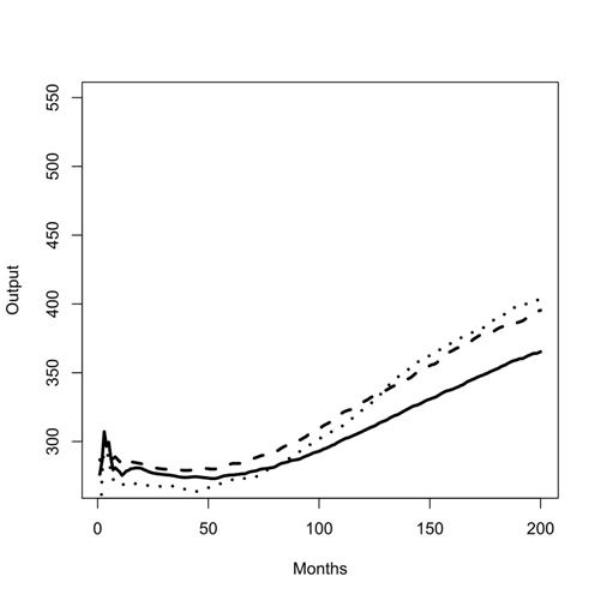
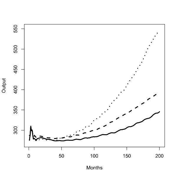
Figure 1. Batch run with zero (left panel) and low (right panel) commuting costs for outputs in uniform low scenario (solid line), uniform medium scenario (dashed line), and low/high scenario (dotted line);

3.7

It can be clearly seen that the relative performance of the two different types of policy distributions depends crucially on the level of commuting costs. If commuting costs are zero, which means that there exists a global labor market without spatial frictions, no significant difference in output growth between the uniform medium and the low/high scenario can be detected. In both cases the policy induced increase in general skills leads to an improved growth rate compared to the uniform low scenario. Quite a different picture emerges for low positive commuting costs. Here the growth rate is substantially larger in the low/high scenario than in the uniform medium scenario and also substantially larger than the growth rate in the low/high scenario without commuting costs. Table 4 shows means and standard deviations of the output variable at t = 50, t=100, t=150, and t=200 which correspond to the discussed figures. In table 5 we statistically test if the differences between the scenarios are significant by applying the Wilcoxon test for equality of means.^[9]

3.8

This finding is remarkable for two reasons. First, it is qualitatively opposite to the effects of the different policy types if commuting costs are large. As discussed in Dawid et al. (2008) for large commuting costs a uniform distribution of skill upgrading measures leads to higher growth than a spatially concentrated policy. Second, if the spatially concentrated policy is implemented the introduction of small spatial frictions on the labor market actually improves performance compared to a frictionless global labor market. Both observations are at first sight surprising and demonstrate the non-linear and path-dependent nature of the relevant economic processes.

3.9

In order to get a better understanding of the economic mechanisms responsible for relative performance of the two policy types we examine in more detail the features of the dynamics of several key variables in the low/high scenario. We always simultaneously consider the cases comm = 0 and comm = 0.05, since such a comparison highlights the mechanisms that are driving the results.

3.10

Figure 2 shows the dynamics of the aggregate output of producers in the low skill region 1 and the high skill region 2. Whereas with no commuting costs both regions produce about the same output, in case of low commuting costs the low skill region exhibits a strong growth in output over time and at the end of the considered time interval of 200 months produces about double the output of the high--skill region. To understand why the output of the high skill region is not larger than that of the low skill region, it has to be kept in mind that the terms high and low skill regions refers to the skills of the workers living in a certain region rather than to the skills of workers working in a certain region.

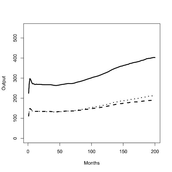
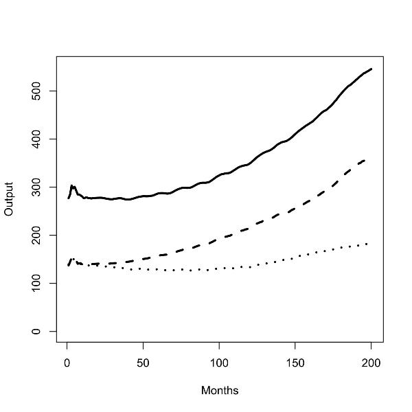
Figure 2.Batch runs for zero (left panel) and low (right panel) commuting costs; total outputs (solid line), output in the low skill region (dashed line), output in the high skill regions (dotted line);

Table 4: Snapshots of average output for the three skill scenarios and two commuting cost levels. (Standard deviations in parentheses.)
comm = 0
Month	50	100	150	200
low/ low	293.95 (6.17)	305.28 (22.09)	330.79 (35.02)	365.27 (55.66)
medium/ medium	280.20 (8.90)	309.63 (23.03)	355.10 (38.86)	395.36 (84.66)
low/ high	266.40 (6.05)	301.67 (36.41)	362.77 (78.13)	402.71 (169.30)
comm = 0.05
Month	50	100	150	200
low/ low	274.07 (4.13)	283.74 (15.33)	306.17 (27.67)	345.80 (42.06)
medium/ medium	280.75 (8.92)	300.31 (21.11)	342.10 (37.63)	393.48 (59.81)
low/ high	281.35 (8.17)	324.55 (47.50)	410.61 (130.00)	545.70 (451.20)

Table 5: Test for statistically significant differences between the output levels of the skill scenarios by pairwise comparison: p values of the Wilcoxon rank sum test.
comm = 0
Month	50	100	150	200
low/ low vs. medium/ medium	<0.0001	<0.0001	0.0008	0.0133
low/ low vs. low/ high	<0.0001	0.6016	0.0677	0.0206
medium/ medium vs. low/ high	<0.0001	0.0058	0.4616	0.7028
comm = 0.05
Month	50	100	150	200
low/ low vs. medium/ medium	<0.0001	<0.0001	<0.0001	<0.0001
low/ low vs. low/ high	<0.0001	<0.0001	<0.0001	0.0002
medium/ medium vs. low/ high	0.4535	0.0254	0.007	0.3252

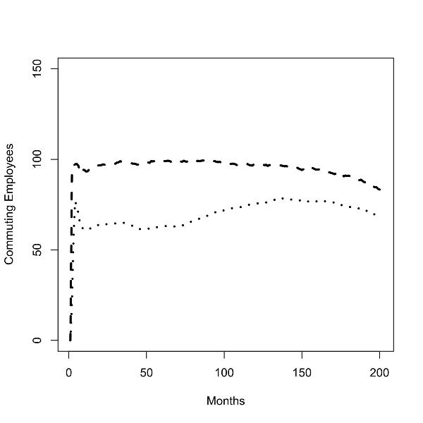
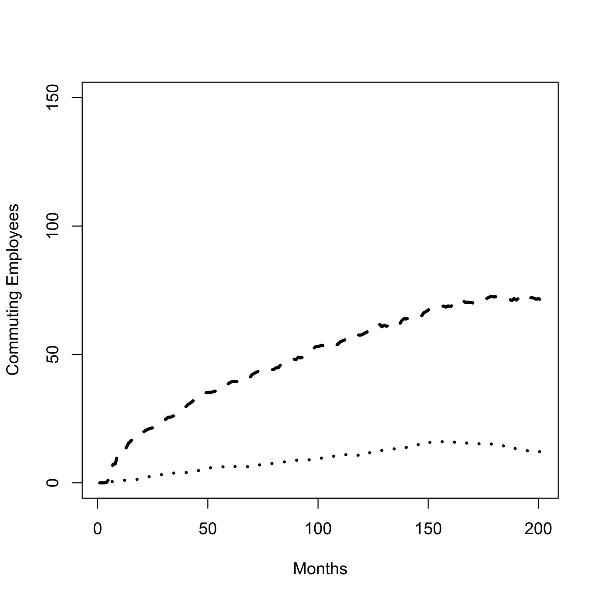
Figure 3.Batch runs for zero (left panel) and low (right panel) commuting costs; number of commuters from low to high skill region (dotted line), number of commuters from high to low skill region (dashed line);

3.11

As can be seen in figure 3 in both scenarios a substantial number of high-skill workers commute to the low-skill region and work for producers located there. In case of no commuting costs almost half of the high skill workers commute throughout the entire time interval of 200 periods, so the number of high-skill employees in both regions is almost identical which also explains the relatively homogeneous output quantities across the two regions. Also, without commuting costs there is a substantial number of commuters from the low-skill to the high-skill region. As has to be expected the introduction of small commuting costs reduces the flow of commuters in both directions, where the number of commuters from the high- to the low-skill region is still substantial and increasing over time. On the other hand, the flow from the low- to the high-skill region becomes very small. So, a first observation to be made is that as well with zero as with small commuting costs substantial transregional spillovers through the labor markets emerge and both regions profit from the general skill level of workers in the high skill region.

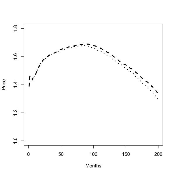
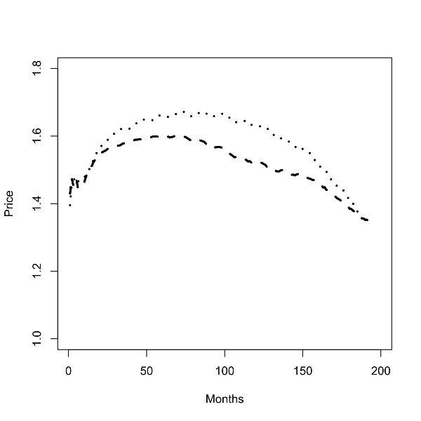
Figure 4. Batch runs for zero (left panel) and low (right panel) commuting costs; prices in the low skill region (dashed line), prices in the high skill region (dotted line);

3.12

The fact that these spillovers have a much more positive effect in the low skill region if commuting costs are positive is due to the different demand dynamics emerging for different commuting costs. Differences in demand for goods produced in the two regions are triggered by price differences which again are driven by wage differences in the two regions. In case of a global labor market no systematic wage differences between the two regions emerge and as can be seen in figure 4 there are no significant price difference between the goods produced in the two regions. In the case of positive commuting costs systematic price differences emerge after a short initial phase, where products from the low-skill region are cheaper than those from the high-skill region. The reason is that initially the number of commuters from the high- to the low-skill region is small and therefore the vast majority of workers with high general skills work for producers in the high-skill region. On the one hand, this leads to a faster wage dynamic in that region because employers have preferences to hire high-skilled workers and therefore these workers are more likely to carry out successful on-the-job searches, thereby increasing their wages^[10]. On the other hand, initially the difference in specific skills between workers with different levels of general skills are small and therefore producers in the high-skill region have higher unit-costs than those in the low-skill region. This translates to the observed price difference and due to this price difference demand shifts towards the goods produced in the low skill region. Producers in that region react to the increasing demand by investing in new capital stock (see figure 5, which due to the assumed technological progress in the investment good sector also improves the quality of their capital stock and increase their productivity. This is a self-reinforcing process because improvements in productivity reinforces the price advantages of producers from the low-skill region and generates additional positive demand effects. At the same time the output expansion of producers from the low skill region leads to a transfer of high-skilled workers from the high- to the low-skill region (see figure 3). The reason that we can see a flow of high-skilled workers from the high- to the low-skill region despite of the fact that the average wage level in the high-skill region is higher, is that due to the falling demand for goods produced in the high-skill region labor demand goes down there and high-skilled workers become unemployed. Indeed the capital and labor investment process triggered by the price heterogeneity is the crucial mechanism responsible for the high growth of the low-skill region output. As can be seen in figure 5 no net investment of capital emerges in the case without commuting costs where prices stay almost homogeneous throughout the run.

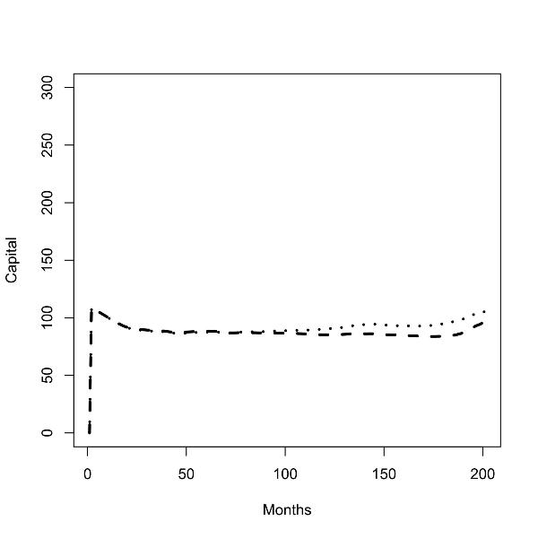
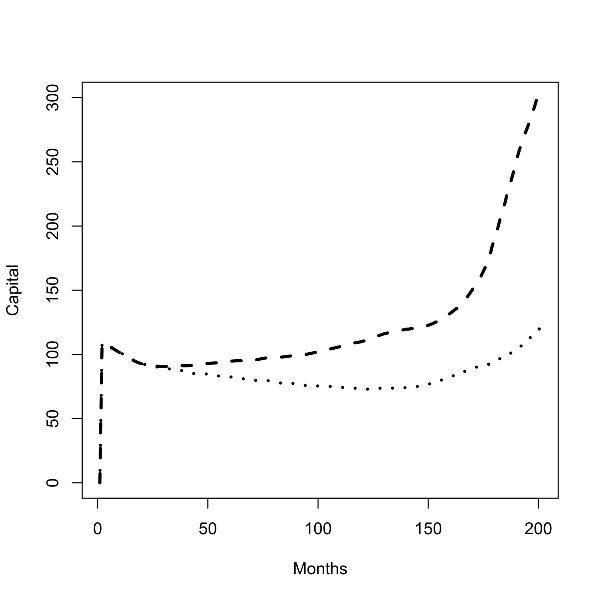
Figure 5.Batch runs for zero (left panel) and low (right panel) commuting costs; capital stock in the low skill region (dashed line), capital stock in the high skill region (dotted line);

3.13

The chain of effects we have discussed above implies that with positive but low commuting costs a self-reinforcing cycle of capital and labor investments by producers from the low-skill region arises which implies that output in that region grows fast and is larger than output in the high-skill region. This however does not imply that in such a scenario the low-skill region also has an advantage with respect to regional income and consumption. As can be seen in figure 6 labor income is in both scenarios larger in the high-skill than in the low skill region, where the difference is smaller in the presence of small positive commuting costs. This of course is due to the fact that high-skilled workers earn higher wages than low-skilled ones regardless of where they are employed. An interesting observation to be made in figure 6 is that labor income in both regions goes up as the commuting costs increase from zero to a positive level. Accordingly, for comm = 0.05 total output in the economy and labor income in both regions are larger than in the absence of spatial frictions in the labor market.

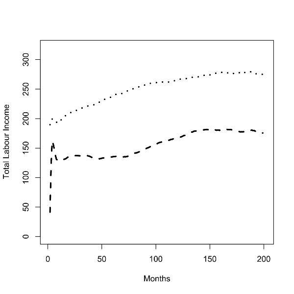
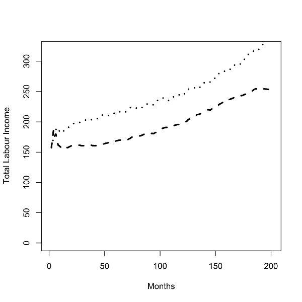
Figure 6. Batch runs for zero (left panel) and low (right panel) commuting costs; total labor income of workers in the low skill region (dashed line) and the high skill region (dotted line).

Policy Implications and Discussion

4.1

In this paper we have used an agent-based spatial macroeconomic model describing the interaction between goods and labor markets to examine the question how the effects of different spatial concentrations of economic policy measures depend on spatial frictions in the labor market. In particular, we have compared scenarios where general skills of workers are upgraded uniformly across regions with regionally concentrated upgrading. It has been shown that in the absence of commuting costs the spatial distribution of the policy measures does not significantly affect their impact. However, if commuting costs are positive but low then a spatially concentrated policy performs better than a uniform approach. In case such a policy is applied the existence of spatial frictions has positive effects on total output in the economy and on labor income in both regions. These positive effects are due to the combination of technological spillovers to the low-skill region through the labor market and demand induced investment incentives for producers in that region. As has been shown in Dawid et al. (2008) the advantages of the spatially concentrated policy disappear if commuting costs become larger and the technological spillovers are reduced.

4.2

These insights have several policy implications. First, they clearly demonstrate that the optimal spatial distribution of policy measures depends crucially on the spatial frictions in different markets. As our results demonstrate the effect of an increase in a parameter like the commuting costs is not always monotonous and therefore a good estimate of such frictions is needed to give sound policy advise. Second, if we take the spatial skill distribution as given and consider policy measures aiming at the reduction of spatial frictions on the labor market, our findings suggest that in cases where skill distributions differ between regions it is desirable to reduce commuting costs to a level where substantial spillovers between regions through the labor market can arise, but it is not necessarily desirable to completely eliminate the spatial frictions. The finding that the existence of frictions can have positive macroeconomic effects is to our knowledge an innovative observation in this type of literature. As has been demonstrated in our discussion above it is due to the combination of the explicit consideration of agents' heterogeneities and of the path dependencies of transient dynamics on the goods and labor market. In that respect we feel that these observation very well illustrate the potential of agent-based models to produce innovative insights into economic dynamics and policy design.

Acknowledgements

This work was carried out in conjunction with the EURACE project (EU IST FP6 STREP grant 035086) which is a consortium lead by S. Cincotti (Universita di Genova), H. Dawid (Universität Bielefeld), C. Deissenberg (Universite de la Mediterrane), K. Erkan (TUBITAK National Research Institute of Electronics and Cryptology), M. Gallegati (Universit Politecnica delle Marche), M. Holcombe (University of Sheffield), M. Marchesi (Universita di Cagliari), C. Greenough (STFC - Rutherford Appleton Laboratory).

Notes

¹The posted worker act should protect the German workers from low wage competition. Commuters from especially Eastern Europe must be paid according to the German wage standards.

²It includes that Polish workers can obtain an unrestricted work permit in Germany. This permit is available for a border region of 50 km as long as the commuters reside in their home country and do not work more than two days per week in Germany.

³In the fully fledged EURACE model, a financial and a credit market will be added, and an exogenous energy market will constitute a proxy for the link to the 'rest-of-the-world' by affecting the production costs in the capital goods market.

⁴In the model each week consists of 5 days and each month of 4 weeks. Accordingly, each year has 240 days.

⁵In contrast, in the fully fledged EURACE platform, there is an explicit credit market model which can be appropriately linked to the real sectors considered here.

⁶In a more elaborate version savings will also be made dependent on the uncertainty over income.

⁷See http://epp.eurostat.eu.

⁸See, for instance, http://www.sachverstaendigenrat-wirtschaft.de/timerow/tabdeu.php.

⁹Note, that the differences between the low/high and medium/medium scenario for comm = 0.05 are significant until period 180 (at a level of significance of at least 90%). After period 180 the variance of the distribution sharply increases so that equality of means cannot be rejected based on the relatively low number of runs we performed.

¹⁰Due to space constraints we do not present the graph that demonstrates the wage differences between the regions.

References

AGHION, P., Blundell, R., Griffith, R., Howitt, P., and Prantl, S. (2006). The effects of entry on incumbent innovation and productivity. NBER Working Paper No. 12027.

ALECKE, B. and Untiedt, G. (2003). Pendlerpotentiale in den Grenzregionen an der EU-Aussengrenze. Beitrag zur International Summer School Economics of EU-Enlargement, University of Hohenheim.

ARGOTE, L. and Epple, D. (1990). Learning curves in manufacturing. Science, 247:920-924.

BASSANINI, A. and Scarpetta, S. (2002). Does human capital matter for growth in OECD countries? A pooled mean group approach. Economics Letters, 74(3):399-405.

BLACK, M. (1981). An empirical test of the theory of on-the-job-search. The Journal of Human Resources, 16:129-141.

BUNDESAMT, S. (2004). Volkswirtschaftliche Gesamtrechnung.

BUNDESAMT, S. (2006). Fachserie 18, 1.4 Inlandsproduktberechnung - Detaillierte Jahresergebnisse 2006.

BURDA, M. and Mertens, A. (2001). Estimating wage losses of displaced workers in Germany. Labour Economics, 8:15-42.

DAWID, H., Gemkow, S., Harting, S., Kabus, K., Neugart, M., and Wersching, K. (2008). Skills, innovation, and growth: an agent-based policy analysis. Journal of Economics and Statistics, 228:251-275.

DEATON, A. (1991). Saving and liquidity constraints. Econometrica, 59:1221-1248.

DEATON, A. (1992). Houshold saving in LDCs: Credit markets, insurance and welfare. Scandinavian Journal of Economics, 94:253-273.

DEISSENBERG, C., van der Hoog, S., and Dawid, H. (2008). Eurace: A massively parallel agent-based model of the European economy. Applied Mathematics and Computation, 204:541-552.

DIW (1994). Ost-West-Pendeln gehört zur Normalität des gesamtdeutschen Arbeitsmarktes. DIW-Wochenbericht, 51-52:861-866.

GEDDES, A. (2003). Still beyond fortress Europe? Patterns and pathways in EU migration policy. Queen's papers on Europeanisation, 4.

GUADAGNI, P. and Little, J. (1983). A logit model of brand choice calibrated on scanner data. Marketing Science, 2(3):203-238.

HILLIER, F. and Lieberman, G. (1986). Introduction to Operations Research. Holden-Day.

JOVANOVIC, B. and Nyarko, Y. (1995). A Baysian learning model fitted to a variety of empirical learning curves. Brooking Papers on Economic Activity, Microeconomics, 1995:247-305.

KIRMAN, A. (1992). Whom or what does the representative individual represent? Journal of Economic Perspectives, 6:117-136.

KRISHNAMRUTHI, L. and Raj, S. P. (1988). A model of brand choice and purchase quantity price sensitivities. Marketing Science, 7:1-20.

NAGLE, T. (1987). Strategy and Tactics of Pricing. Prentice Hall.

OECD (2004). Benefits and Wages: OECD indicators.

PISSARIDES, C. and Wadsworth, J. (1994). On-the-job-search, some empirical evidence. European Economic Review, 38:385-401.

ROSENFELD, C. (1977). The extent of job search by employed workers. Monthly Labor Review, 100:39-43.

SJAASTAD, L. (1962). The costs and returns of human migration. The Journal of Political Economy, 70(5):80-93. Part 2: Investment in Human Beings.

SMALL, I. (1997). The cyclicality of mark-ups and profit margins: Some evidence for manufacturing and services. Bank of England Working Paper.

TESFATSION, L. and Judd, K. E. (2006). Handbook of Computational Economics II: Agent-Based Computational Economics. North-Holland.

Return to Contents of this issue

© Copyright Journal of Artificial Societies and Social Simulation, [2009]