
 Abstract
- The pioneering works in Agent-Based Modeling (ABM) - notably Schelling (1969) and Epstein and Axtell (1996) - introduced the method for testing hypotheses in "complex thought experiments" (Cederman 1997, 55). Although purely theoretical experiments can be important, the empirical orientation of the social sciences demands that the gap between modeled "thought experiments" and empirical data be as narrow as possible. In an ideal setting, an underlying theory of real-world processes would be tested directly with empirical data, according to commonly accepted technical and methodological standards. A possible procedure for narrowing the gap between theoretical assumptions and empirical data comparison is presented in this paper. It introduces a two-stage process of optimizing a model and then reviewing it critically, both from a quantitative and qualitative point of view. This procedure systematically improves a model's performance until the inherent limitations of the underlying theory become evident. The reference model used for this purpose simulates air traffic movements in the approach area of JFK International Airport in New York. This phenomenon was chosen because it provides a testbed for evaluating an empirical ABM in an application of sufficient complexity. The congruence between model and reality is expressed in simple distance measurements and is visually contrasted in Google Earth. Context knowledge about the driving forces behind controlled approaches and genetic optimization techniques are used to optimize the results within the range of the underlying theory. The repeated evaluation of a model's 'fitness' - defined as the ability to hit a set of empirical data points - serves as a feedback mechanism that corrects its parameter settings. The successful application of this approach is demonstrated and the procedure could be applied to other domains.
- Keywords:
- Empirical Modeling, Genetic Optimization, Falsification
Introduction
- 1.1
- Important methodological and theoretical contributions to connecting ABM to the social sciences were made throughout the 1990s (see for example Epstein and Axtell 1996). In a prototypical application, researchers test proposed micro-behavior in fully formalized "complex thought experiments" (Cederman 1997, 55) to observe the emerging macro-structures.
- 1.2
- Empirically-oriented social scientific theories nevertheless rely on explanation—whether formalized or not—that explicitly takes real-world data into account. In an ideal setting, an underlying theory of real-world processes would be tested directly with empirical data, according to commonly accepted technical and methodological standards. In computational modeling, these standards are lacking today. Moreover, the discussion about the role of Agent-Based simulation within the social sciences seems to be far from over. Heine, Meyer and Strangfeld (2005) argue that promoters of this research method must still convince conservative representatives of the social sciences regarding two important aspects: The scientific benefit of computer simulation and prevention of arbitrariness in modeling real-world phenomena.
- 1.3
- The scientific benefit of simulation-based methods has been demonstrated in a wide array of applications, ranging from the simulation of settlement patterns of a North American Indian tribe (Dean et al. 2000), nation building and dissolving processes in European history (Cederman 1997), studies in asymmetric and guerrilla warfare (Geller 2006), and optimization attempts in road traffic (for example Kumar and Mitra 2006). Nevertheless, the prevention of arbitrariness is a less frequently discussed problem.
- 1.4
- This paper discusses a general evaluation technique for empirical ABM. This mechanism configures a given model's parameter settings to achieve close-to-optimal congruence with empirical data. The optimized settings are used to highlight the abilities and limitations of the underlying theory. It will be shown how a naive ad hoc explanation of a complex real-world phenomenon can be automatically tuned to reproduce a sequence of empirically recorded events within its theoretical limitations. This opens up a way of critically assessing the model's abilities and limitations (both quantitatively and qualitatively). Moreover, the explanatory power of different model mechanisms (e.g. the specified behavioral rules for the agents) can be tested in the competitive setup of genetic optimization techniques: Rules that help to increase the overall 'fitness' of a model's configuration will have an evolutionary advantage over others. The 'fitness' is defined as the model's ability to reproduce an empirical record with its own simulation results. A comparative measurement of the ability to reproduce an empirically recorded trajectory enables researchers to determine whether the model's performance is inferior or superior to other potential explanations for real-world phenomena modeled on the basis of other assumptions. Falsification in the circle of progress - perceived as a precondition of scientific endeavor (see: Popper 1966, 15) - plays a central role in the theoretical foundation and technical implementation of this procedure.
- 1.5
- The aim of this study is to propose and demonstrate a way 'closing the loop' between theoretical explanation, modeling, automated optimization, and comparison to empirical data, followed by theoretical reconsideration. Sophisticated methods have been proposed for several steps within this loop, the theory-model translation and the model-reality agreement. Especially Pontius' (2001) approach to the evaluation of land change models is an important contribution to model evaluation; this approach is based on the analysis of the 'Relative Operating Characteristic' of a given model. Moreover, several publications apply the notion of 'stylized facts' to the creation and analysis of ABM (for example: Shimokawa, Suzuki and Misawa (2007); Heine, Meyer and Strangfeld (2005)). This study only utilizes a simple theory and straight-forward goodness-of-fit measurement, but more advanced methods and theories could be used with the same framework.
- 1.6
- A practical obstacle in this procedure is the potential lack of high resolution real-world data. A rich data base is a necessary condition for tuning the model in the optimization runs. To account for this problem, a highly transparent and well-documented phenomenon was chosen as the subject of research. Data acquisition was further simplified by the fact that all relevant information was digitally accessible. For demonstration purposes, this presented procedure was moved into a barely technical domain because of its supreme data supply. The approach is nevertheless applicable to social scientific questions.
Falsification
and Progress
- 2.1
- Although ABM is widely applied in a variety of applications it still lacks one important aspect of scientific theories: falsification, or the ability to disprove a given explanation. In the field of ABM, reliable model evaluation and falsification are especially hard to accomplish. The discussion of suitable falsification-mechanisms for this domain is thus very important in addressing the problem of arbitrariness. The identification of inaccurate theoretical explanations through simulation can help to prevent arbitrary postulates from being accepted by the research community. Earlier theoretical attempts have been made to extend the falsification concept towards complex phenomena: Hayek (1972) underlines the necessity of trading some of the advantages of a clear falsification for the possibilities of doing research on complex phenomena:
- 2.2
-
While it is desirable on the one hand to keep our theories as falsifiable as possible, we also have to advance into areas in which the degree of falsifiability declines necessarily. This is the price we have to pay for our advance into the area of complex phenomena (Hayek 1972, 18) (translation mine).
- 2.3
- In further developing his point, Hayek turns towards Darwin's theory of natural selection as a reference theory of complex phenomena. He underlines that this theory is not just about a specific order in the development of the species, but about defining a principle that underlies the developmental process. In Agent-Based Models, the specified micro-behavior fulfills this role of a general development principle of the system. Darwin's theory does not comply with Popper's principle of forecast and control as a condition for falsification since it only describes the underlying rules in a complex process independent of specific states. Darwin himself pointed out that "all the labour consists in applying this theory" (Hayek 1972, 22). Hayek goes on to construct cases in which Darwin's theory of natural selection could be disproved:
- 2.4
-
[...] if we did observe a sequence of events that could not be matched into its pattern [the pattern of the theory of evolution]. If for example horses did give birth to foals with wings, or if the amputation of a dog's paw led to successive generations of paw-less dogs, this theory would have to be considered disproved. [...] The scope of what is permitted by this theory is incontrovertibly large. One could nevertheless say that only our limited imagination prevents us from realizing how much bigger the scope of the forbidden is - how infinite the variety of the thinkable forms and organisms that will not appear on earth in a foreseeable time, according to the theory of evolution (Hayek 1972, 23) (translation mine).
- 2.5
- Hayek's proposal for evaluating complex theories focuses on a necessary addition to the quantitative evaluation: If an Agent-Based Model - which formally expresses a theory - shows properties that simply contradict the principles of the observed dynamics, it must be considered wrong or incomplete. Falsification in modeling complex phenomena can be achieved with a mixture of quantitative and qualitative measures applied to the modeled phenomenon. A suggestion for a quantitative evaluation method is given in (Epstein 2006, 91):
- 2.6
-
The degree of fit between a model and real-world situations allows the model's validity to be assessed. A close fit between all or part of a model and the test data indicates that the model, albeit highly simplified, has explanatory power. Lack of fit implies that the model is in some way inadequate. Such "failures" are likely to be as informative as successes because they illuminate deficiencies of explanation and indicate potentially fruitful new research approaches.
- 2.7
- Both Epstein's quantitative and Hayek's qualitative approach will be applied in the evaluation of the implemented reference model.
Identifying Scientific Applications for Agent-Based Modeling
-
The Theoretical Approach
- 3.1
- Earlier simulation attempts in ABM aimed at providing test environments for the complex interactions of proposed micro-behavior. Epstein (2006) introduced the term 'generative sufficiency' in this context to characterize the research goal ABM:
- 3.2
-
Classical emergentism holds that the parts (the microspecification) cannot explain the whole (the macrostructure), while to the agent based modeler, it is precisely the generative sufficiency of the parts (the microspecification) that constitutes the whole explanation! [...] Classical emergentism seeks to preserve a "mystery gap" between micro and macro; Agent-Based Modeling seeks to demystify this alleged gap by identifying microspecifications that are sufficient to generate - robustly and replicably - the macro (whole)(Epstein 2006, 37).
- 3.3
- This research aim has been pursued in several successful projects in Agent-Based Modeling, and one representative and heavily-cited example of this type will be briefly introduced in this section. This introduction serves as an entry point for the definition of a more empirically-oriented research goal.
- 3.4
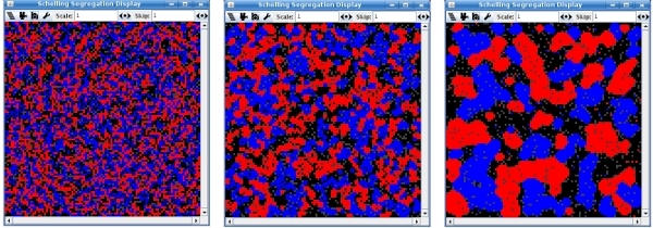
- The identification of 'microspecifications' that reliably give rise to emergent patterns of interest has already been demonstrated in Schelling (1969). Based on the configuration of neighborhood preferences, Schelling was able to show the emergence of segregated settlement patterns. [1]
- 3.5
- Figure 1
below shows advanced states
of a reimplemented Schelling-model with preference values 1, 2
and 3.[2]
The emergence of distinct settlement patters can be seen in this
screenshot. The explanatory power of the model derives from the fact
that distinct macro constellations can be reproduced on the basis
of micro decision making.
- 3.6
- The implementation of the 'generative sufficiency' concept is constructed around human observers as the judging instance. These observers analyze real world-phenomena based on their personal insights or explanations from the literature. They then translate the resulting theory into model mechanisms, run the model, and analyze the result. In this case, a sufficient generative explanation is given in terms of distinct settlement patterns that a human observer would classify as 'segregated' or 'non-segregated'. Different parameters and initial conditions in Schellings' model lead to either of large, roundish aggregations of agents or to a well-mixed population. The emergent pattern, as judged by the human observer, is not equivalent to one specific system state.
- 3.7
- The basic research question of generative sufficiency is therefore: Can my microspecifications lead to a large set of system states that a human observer would classify as the emergent pattern of interest? This is obviously not a very hard criterion as such. It nevertheless enables researchers to run computer-aided theoretical experiments and compare the resulting phenomena to real-world observations. Furthermore, efforts were made to calibrate models according to empirical findings.
-
The Empirical Approach
- 3.8
- In a recent attempt to apply empirical evaluation techniques to the field of Agent-Based Modeling, various approaches have been discussed. Boero and Squazzoni (2005) refer back to the Artificial Anasazi project (Dean et al. 2000) as a good example of incorporating a large amount of empirically recorded data into a simulation. This model aimed at providing an explanation for the disappearance of a native North American tribe from a specific settlement site that was inhabited for centuries until the late thirteenth century. The environmental conditions for living and farming for this site were modeled, based on existing data sets.
- 3.9
- A rich paleoenvironmental record, based on alluvial geomorphology, palynology, and dendroclimatology enabled an accurate quantitative reconstruction of annual fluctuations in potential agricultural production, calculated in kilograms of maize per hectare (Gumerman 1988). This potential production estimate was the basis for creating a dynamic "production landscape" (Epstein 2006, 94), which served as a digital model of Long House Valley and featured temporally and spatially changing crop yields. Nutrient contents of different soils and drought were taken into account for estimating this potential production value. Numerous studies (especially Dean 1966, Dean 1969; and Dean et al. 1985) were taken into account to optimize the accuracy of this approximation. The assiduous identification of statistical relations between the soil attributes, drought, and the resulting production of maize in kilograms per hectare eventually provided a dynamic model of crop yields, based on the known environmental conditions.
- 3.10
- Moreover, successor cultures of this specific Anasazi tribe provided anthropological insight into the social and demographic mechanisms in place. Taken together, the accurate identification of micro-mechanisms enabled the simulation to reliably produce general trends in the population size over the simulated centuries, which realistically reflected the archaeological record. The model was nevertheless not capable of explaining the sudden abandonment of the site of interest. It also failed to reproduce the exact magnitudes in the population dynamics. These explanatory limitations of the model are important research results. They can lead the way for subsequent modeling and help researchers to critically review the underlying theoretical assumptions.
-
Empirically-Guided Parameter Tuning
- 3.11
- The following procedure can be seen as a synthesis between the empirical and the theoretical approach. Instead of simulating the general dynamics of a complex phenomenon based on pure theory, it is oriented towards a rich data set. In contrast to the empirical approach as used in the Artificial Anasazi project, it does not aim at the empirical evaluation of all assumed micro-mechanisms involved. Instead, it aims at heuristically searching the explanatory scope of the underlying theory to explain the empirical findings.
- 3.12
- The research question to be solved with this approach is to what extent an empirical trajectory of events can be explained by the micro-mechanisms in place. Compressed into one sentence, the new research question is: To what extent can the empirically recorded sequence of events be explained by my model?
- 3.13
- To answer this question, the model behavior that is usually defined by hard-coded rules and numerical parameters is automatically optimized in a machine learning procedure. The optimization goal is a reproduction of the empirical data set in a simulation. A heuristic search through the parameter space for a close-to-optimal configuration is therefore performed.[3] The resulting optimized model is then quantitatively and qualitatively compared to the empirical data set. Instead of aiming for a wide range of resulting system states that a human observer would classify into some theoretical category, this setup aims at producing a system state for a given time that is congruent with the corresponding empirical data. Assessing the congruence of model and reality requires a distance function, which in this case is the average spatial distance of an agent to its real-world counterpart at a given time. The fundamental question, whether or not a given theoretical explanation is capable of reproducing an observed sequence of events in a complex phenomenon, can be answered in this way.
Demonstrating the New Approach
-
Air Traffic as a Testbed for the New Approach
- 4.1
- In any attempt to model social events using ABM, researchers face a profound problem: the general lack of high resolution spatio-temporal data for the domain of research. This problem turns the empirically-guided simulation of social systems into a very time-consuming process. The Artificial Anasazi project (Dean, Gumerman, Epstein and Axtell 2000) used an archaeological record that was created over decades. While that project provided a major theoretical and methodological contribution, it relied heavily on the accessibility of archaeological evidence and behavioral observations. Less merciful historical phenomena whose principal actors cannot be observed in vivo and whose traces were wiped out are less accessible by this approach.
- 4.2
- Instead of taking a historical perspective with proposed, but not fully proven, assumptions about the past, this study focuses on a present-day phenomenon to get around the problem of data acquisition. With air traffic being a well-known phenomenon of our time, we are as close as can be to a full description of the processes involved. Nearly real-time data can be retrieved from the Internet, and charts, rules, and radio communication are publicly available.
-
Origins of Data
- 4.3
- Due to the advantages in data supply, the aerial movements of incoming, controlled flights at JFK International Airport were chosen as the subject of research. Single aircraft serve as agents in the simulation. Their behavior is guided by simple rules that are weighted numerically. The data used for building and evaluating the model can be divided into three different types. The first type is general information regarding FAA[4] regulations and IFR-procedures[5] and general ICAO standards.[6] Printed media and Internet sources were combined to gather this required background information. The second type of information included real-time recordings of radio communication from the JFK International tower, the approach sectors CAMRN and KENNEBUCK, and the final approach vector. It was downloaded from http://liveatc.net. This radio communication was not systematically included into the model construction or evaluation. It was sporadically used to investigate special situations and to identify the landing procedures that were used at a given time. In addition to the available ATIS[7] information, weather conditions could be reconstructed whenever they were of special interest.[8] The third and by far most important data source was a five minute delayed estimation of position, ground speed, heading, altitude, and call sign of all inbound IFR-flights to JFK International. This data was downloaded from http://www.fboweb.com in one minute intervals.[9] This website belongs to the web presence of Fboweb, a civil flight tracking service. Several civil flight tracking services in the U.S. offer delayed position estimations for civil aircraft for which a flight plan was filed.
-
Modeled Theory and Genetic Optimization
- 4.4
- Modern civil aviation is a complex phenomenon that is shaped by a wide array of logistical and technical concepts. An adequate model of the processes involved would certainly exceed the assumptions in the presented example theory. This theory is nevertheless adequate for creating a test case for genetic optimization and falsification in empirical ABM.
-
A Suitable Agent-Based Explanation
- 4.5
- For the purpose of demonstrating automated parameter tuning in empirical ABM, a radically simplified and partially false theory of IFR flying is assumed at this point. A good model of IFR procedures would look different than the one presented and would rely on theoretical assumptions that are directly derived from the introduced procedures. It is not the aim of this study to provide a realistic model of controlled flights, but to investigate to what extent it is possible to model IFR arrivals within the Agent-Based paradigm. Therefore, the central control of the ATC over areal movements during the approach is neglected in the model. The agents move by themselves according to numerically weighted rules.
-
Modeling the Theory
- 4.6
- For modeling the theory of self-determined inbound flights, only rudimentary knowledge about flying is taken into account. Apart from the sophisticated but data-invisible procedures, the investigated phenomenon is about airplanes that come from different directions to smoothly touch down at a runway at the JFK airport. A minimal theory which explains this phenomenon should take some basic aspects of this phenomenon into account:[10]
- 4.7
-
1) Aircraft know where the airport is.
2) Aircraft are oriented towards the airport.
3) Aircraft reduce their altitude during the approach.
4) Aircraft reduce their speed during the approach.
5) Aircraft usually land in the upwind direction.
6) Aircraft usually fly a traffic circuit before landing.
- 4.8
- These assumptions appear simplistic in comparison to the real procedures, but they serve the purpose of providing a minimal explanation for the phenomenon. Focusing on minimal explanations is a suitable proceeding for modeling purposes and a common scientific procedure. A realistic coeval theory of flying as given in terms of the FAA Instrument Procedures Handbook[11] obviously includes much more complicated concepts. It is assumed for the purpose of providing an example theory that all these simple driving forces aggregate in guiding an aircraft's movements. Reducing the risk of midair collisions to an absolute minimum is one of the main purposes of controlled procedures. Nevertheless, the ASDI class II data stream[12] only provides position information with a temporal resolution of one minute and a spatial resolution of about one nautical square mile (ca. 1.85 km²). This data sometimes suggests midair collisions, although the referred aircraft are traveling safely in a horizontally and vertically staggered formation. A crash detection or avoidance mechanism was therefore not taken into account.
-
Model Appearance and Usage
- 4.9
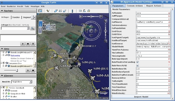
- The RePast 3 API[13] provides easy-to-use functions for creating graphical user interfaces with dynamically updated charts and diagrams for analyzing the model's dynamics over time.
- 4.10
- The screenshot above shows the settings section of the model and the model's appearance in Google Earth.[14]It shows circling aircraft in the demo mode of the model. Google Earth integration was a very important component of the model for comprehensively visualizing the model's performance.
-
Assessing Model-Reality Agreement Quantitatively
- 4.11
- In order to judge the model's ability to capture the spatial patterns of controlled approaches to JFK International, a simple distance measurement was used. The average distance between all agents and their real-world counterparts was calculated in every time step. The duration of a time step in the model corresponds to one minute real-time. This setting was chosen because the ASDI stream offers one minute update intervals.
-
Genetic Optimization
- 4.12
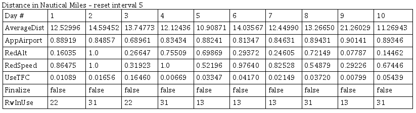
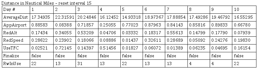
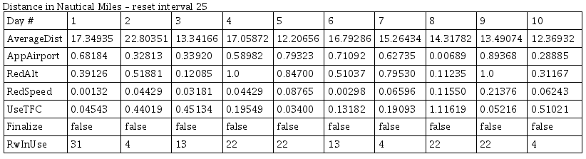
- The model not only uses hard-wired rules for simulating aircraft behavior, but also adjustable parameters (coefficients) for weighting the impact of every single rule.[15] This mechanism enables the exploration of a wide range of different configurations within the same set of applied rules. The space of possible configurations is heuristically searched by means of genetic optimization. The results of any genetic optimization heavily depend on the fitness function in use. After a single set of parameters is tested in its environment (in this case, its ability to move the agents in the model), the fitness function evaluates the resulting performance, squaring the average distance in nautical miles between the agents and their real-world counterparts. A fitness value of 0 would indicate a perfect match between model and reality, while a value of 100 shows an average spatial distance between the empirically recorded and artificially created positions of 100 nautical miles. To get a better overview of the model's performances for different model-reality comparison durations, so-called reset intervals were introduced. The three intervals for 5, 15, and 25 minutes simply move the agents to the positions of their real-world counterparts at the end of an interval. The 25-minute duration roughly corresponds to a whole approach and landing sequence, whereas the shorter interval resets the agents several times during the landing procedure. Thus, a more complete overview of the model's performances was gained.
- 4.13
- For every set of empirical data points and every reset interval, the following procedure was executed: A set of 300 candidate settings (for the model coefficients) was randomly chosen and each of these settings was used in the simulation to guide the agents' behavior. The coefficients were real values in the interval {0,1}. The resulting behavior was compared to the real aircrafts' behavior according to the distance-based fitness function. High ranking settings were then recombined to create another 300 candidate settings, and this cycle was repeated eight times. In the terminology of genetic algorithms, 300 chromosomes were optimized over eight generations. The best chromosome (or the winning candidate settings) of all generations was then used as the optimization result. This also enabled different rules that tried to account for the same behavior to engage in a virtual struggle for survival. Each optimization run was executed for one single day. A day consisted of 500 spatio-temporal position estimations with a temporal resolution of one minute and a spatial resolution of one nautical mile (about 1.85km). All incoming controlled flights to JFK within a model space of 200 nm≤ around the airport were included in the simulation.
- 4.14
- The final evaluation of the model was based on the flight tracking data, including the total number of 5,000 data points collected over ten days. Testing one set of rule coefficients with the collected data of one day took between 7 and 11 seconds (depending on the air traffic) on a 2Ghz AMD Athlon XP workstation using Gentoo Linux. The genetic optimization with the mentioned fitness function, three reset intervals (for 5, 15, and 25 minutes), and the data of ten days took about 180 processor hours.
Results
-
The Quantitative Analysis
- 5.1
- The optimization results regarding the rule coefficients and the model's ability to reproduce the empirical data differs for the different days. This might be surprising at first glance, but the air traffic situation, landing direction, traffic circuit, and the weather conditions also differ. All optimization results can be found in the Appendix. The results themselves do not indicate whether or not the actual goal of reproducing the real traffic patterns was reached. For this purpose, it is more illuminating to use the introduced distance measurements to show the model's performance.
-
How Good Are the Results?
- 5.2
- The plots below show the frequencies for different average
distances
between agents and real counterparts:
Figure 4: Histogram for the average distances in nautical miles between agents and real aircraft for all ten days. Note the different scales. 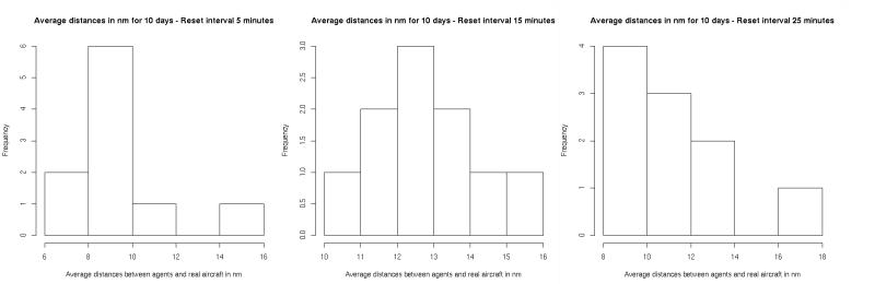
- 5.3
- Average values for the different results are 9.63 for the five minute reset interval, 12.82 for the 15 minute interval, and 10.96 for the 25 minute time frame (with standard deviations of 2.07, 1.53, and 2.26, respectively). It is surprising at first glance that the 25-minutes simulations seem to capture the real movement patterns more accurately on average than the 15-minute runs. A possible explanation for this is that the longer comparison benefits from two very static phases of normal flights: When approaching the airport from a greater distance, airplanes fly more or less straight towards it. In this phase, an aircraft's overall movement can be described nicely with the "Approach Airport" rule. In the last stage of the flight, the aircraft is already very close to the runway. While the real aircraft perform a traffic circuit and the "Approach Airport" rule just guides the agents into the airport from whatever direction it might originate, the distances between agent and aircraft remain comparatively small.
-
How Similar Are the Results for Different Days?
- 5.4
- A closer look at the results indicates that the model's
ability to
capture the real flight movements varies significantly from day to
day. Variation between different reset intervals, on the other hand,
are comparatively
small. The plots below show the optimization results for all ten days,
the three reset intervals, and the squared position fitness function.
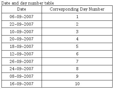
Figure 5: Average distances in nautical miles for the ten days (the corresponding dates can be found in the Appendix). Note the different scales. 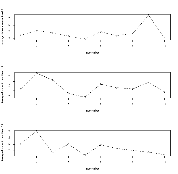
- 5.5
- A comparison of these three plots shows the relative resemblance between the results of the 15-minute reset interval and the 25-minute setting. The Pearson-correlation between the 5- and the 15-minute interval is 0.55, and 0.58 for the 15- and 25-minute conditions.
-
What Affects the Model's Performance?
- 5.6
- The optimization results have proven to be fairly robust towards changes in the reset interval setting. Based on this observation, the really interesting discussion can be started. What affects the model's performance in resembling reality?
- 5.7
- This question can be answered by focusing on a particular day in the analysis. An average performance over all three reset intervals for all ten days was calculated which revealed that day 2 was the hardest to approximate. It shows an average spatial distance for all reset intervals of 14.07 nautical miles. The average value for the nautical distance-based approximation is 11.14 and the standard deviation is 1.48. Day 2 is about two standard deviations worse than the average case. Day 2 corresponds to September 22, 2007. Weather data from "Weather Underground" (http://www.wunderground.com) was reviewed for all simulated days.[16] The weather was very good for 8 of these days, yielding visibility ranges of more than 10 kilometers. September 22, on the other hand, was a difficult day for flying. Rain and fog temporarily limited visibility below one kilometer. Throughout most of the day, the temperature on the ground was only one degree centigrade above the dew point so that clouds and fog developed already at very low altitudes.
- 5.8
- Weather conditions were completely invisible to the model and were not taken into account in the simplified underlying theory. Why would the model's ability to resemble the observed patterns decrease so dramatically on a day like that? First of all, one must consider that it is a major technological and mental challenge to land a commercial jetliner safely in minimal visibility. A large number of technical aids are needed to perform this task. With a visibility below one kilometer it is usually necessary to perform a so-called category III ILS landing. A category III ILS landing is usually a manually flown approach followed by a completely automated landing which requires a specially trained pilot. The plane also has to be specially equipped. Some insufficiently equipped airplanes were simply diverted to other airports that day. Other incoming flights were commanded to fly holding patterns. Aircraft that circle at a given spot or that even depart from the airport were simply beyond the underlying theoretical assumptions and thus show the limitations of these assumptions.
- 5.9
- There is a striking parallel to the Artificial Anasazi Project in this regard. Archaeologically invisible driving forces are assumed to be responsible for the final abandonment of the investigated settlement site. These driving forces are clearly beyond the underlying theoretical explanation of the Anasazi Model. The model therefore contradicts the reconstructed Anasazi history at a certain point. The Artificial Airplanes behave in a very similar way: Under specific conditions that are invisible to the model, they start contradicting reality. Deviated aircraft of September 22 were used as archetypes for their much simpler agent-counterparts. But while they were moving away from JFK, the simple agents had no other choice than to approach the airport, because this behavior was an axiomatic assumption of the underlying theory.
-
The Qualitative Analysis
- 5.10
- Valuable insights into the model's performance can also be gained from a more qualitative point of view. For this purpose, various common traffic situations were observed in both model and reality. These situations were then contrasted and discussed using background knowledge of the procedures in use. The sometimes criticized approach of doing potentially insignificant case studies to explore the shape of social phenomena can be valuable for the evaluation of Agent-Based Models: Digital 'case studies' provide insight into the behavioral differences between a real-world phenomenon and model. Differences in behavior between model and reality can highlight the limits of the theoretical explanation that underlies the model. In every single instance, they highlight the inequalities between model and real phenomenon. Of course, these functional differences do not necessarily deem the model a bad approximation, but they can lead to systematic extensions of the model.
-
Close to the STARs
- 5.11
- The model is capable of roughly simulating typical aircraft
movements
in remote distances to the airport. When aircraft approach an
international airport to land under instrument flight rules they
usually travel on predefined routes along a number of fixed waypoints.
These routes
are called "standard terminal arrivals", or STARs. Oriented
along a track of radio navigation related waypoints, STARs do not
provide a straight path to the airport. Instead, they provide a
horizontal
margin between incoming flights from different directions and they
are easy to follow from a navigational point of view. The STARs in
use can be assigned by ATC to individual aircraft or can in some cases
be chosen by the pilot.[17]
- 5.12
- When looking at the map of a STAR, it is striking that
these routes
lead to the airport in a fairly straightforward but not completely
optimal manner, since they force the aircraft to perform multiple
changes
in direction en route to the airport. This behavior is not part of
the model. The artificial aircraft simply approach the airport on
a great circle course -- that is, the shortest possible route on or
above the surface of the planet. These different behaviors of the
real airplanes and the artificial ones lead to small differences in
the agent routes. The pictures below illustrate the effect.
Figure 6: The picture on the left shows the horizontal margin between two different STARs. A closer look on the right side (this time over Long Island) shows the growing distance between aircraft and agent. The agent approaches JFK following the great circle bearing, and the aircraft performs a STAR and enters the traffic circuit. 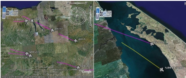
- 5.13
- In most cases, the approximation of STARs by means of the "Approach Airport" rule is fairly accurate. Although the STARs do not exactly follow the great circle bearing, they are designed to bring the inbound traffic to its destination in a "close to optimal" way. The real problem of the model in capturing specific operations can be found in other aspects than the remote approach movements.
-
Unaware of Deviations and Holdings
- 5.14
- The weather situation on September 22 has already been
discussed in
subsection [5.4].
Even worse conditions were
observed on August 8, a day that featured low visibility, heavy winds,
and thunderstorms. The picture below was taken at 6:59 am (New York
local time EDT). For this time, the weather report shows a visibility
of 1.2 km. Many incoming flights were circling and waiting for the
weather to improve, while the agents approached the airport as usual.
Figure 7: Inbound flights performing holdings in the early morning hours of August 8, 2007. The displayed agents are unaware of the weather conditions and approach the airport as usual. 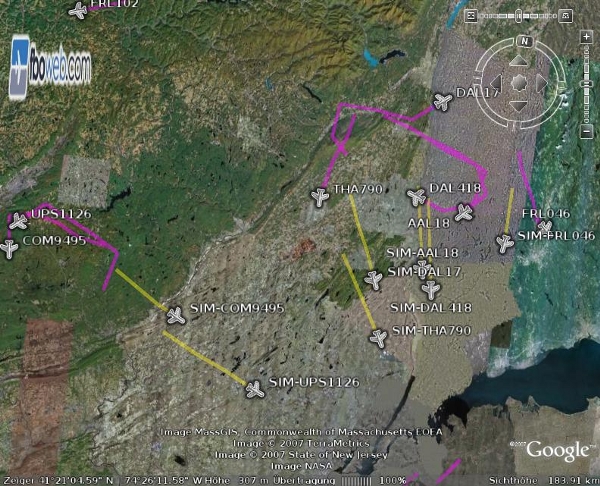
- 5.15
- The significant differences in the model-reality agreement were revealed both statistically and visually. This situation clearly demonstrates that the fundamental theoretical axiom of aircraft always approaching the airport can be wrong under specific circumstances. Similar theoretical limitations seem to be immanent to the Artificial Anasazi Project. One of these axioms is that the Anasazi households stay where they are as long as the supply situation allows it, or for a maximum period of thirty years. Nevertheless, the real Anasazi disappeared, although one third of the population could have remained in the valley. The limitations of the underlying micro-behavioral assumptions are clearly uncovered in these modeling attempts. These limitations point to necessary future enhancements of the models.
-
Sharp-Edged Traffic Circuits
- 5.16
- The "Fly Traffic Circuit" rule was designed to offer a more
realistic procedure for the final approach. As the result tables in the
Appendix show, the "Approach
Airport" rule was favored by the fitness function over the more
complicated traffic circuit rule. A simple explanation for this is
that the real traffic circuits are adapted to the flying conditions
on a daily basis. These are also larger and smoother than the simple
rectangular prototype. The pictures below contrast artificial and
real traffic circuits.
Figure 8: Real and artificial traffic circuits in a direct comparison. The artificial airplanes are on the left and the real ones on the right. The artificial traffic circuit is smaller and the agents fly sharp-edged curves. Note that the landing direction differs in these screenshots (310∞ for artificial airplanes and 220∞ for the real ones). 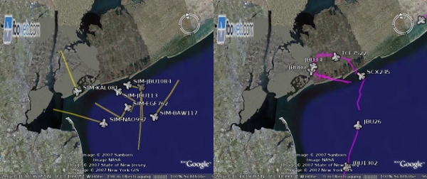
- 5.17
- In many cases, landings at JFK take place at the same time in two different directions. The 22 left and the 13 left runways, for example, can be safely operated at the same time, given a suitable wind direction. This case was not considered in the design of the "Use Traffic Circuit" rule. Although the simpler straight approach was favored over the more complicated curved approach, this rule was not useless. It provides a special and very interesting case for genetic optimization: Two contradicting behaviors for the same aspect of the model, the simulation of the final approach, were offered to the genetic algorithm. In almost all cases of finished optimizations, one of these rules was set to 0 while the other was actively used with a setting of around 0.8. This offers an interesting additional option for using genetic optimizations: Instead of evaluating whole theories, single aspects of the desired behavior can also be evaluated. Using a suitable fitness function, different explanations for the same aspect of the model can compete in the optimization process with the "fittest", e.g. most suitable, rule prevailing. In this case, the static proposal of a rectangular traffic circuit produced poorer results than the straight approach, according to the distance measurements in use. Other fitness functions could have a numerically rewarded rule set that chooses the right landing direction. In this way, the "traffic circuit" rule could have gained an advantage over the simpler straight approach.
-
Head-on Landings
- 5.18
- While the slight inaccuracy in following the STARs and the
general
unawareness of holding patterns are forgivable drawbacks of the model's
behavior, the straight approach poses a serious problem. When agents
from different directions simply head straight for the airport, they
do not necessarily land in the appropriate directions of the runways.
Even worse, agents land head-on with other agents. The picture below
shows this completely unrealistic behavior.
Figure 9: Head-on landings from all directions. The "Finalize After Landing" rule was switched off to get this shot. 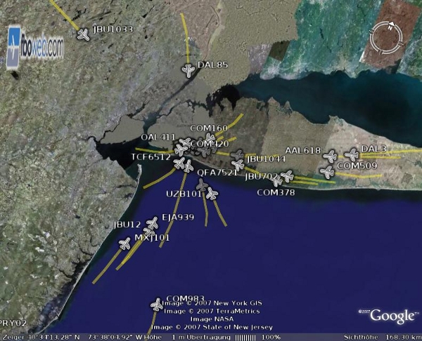
- 5.19
- There have been isolated, tragic incidents of runway collisions of commercial airliners in the history of civil aviation. Nevertheless, it does not happen 100 times a day at JFK International. With this situation contradicting the reality of aviation so fundamentally, Hayek's (1972) proposal for falsifying complex theories (as discussed in section [2]) can finally be applied.
- 5.20
- We now have a situation in which the proposed and modeled theory of flying contradicts the reality of flying in a fundamental way. Darwin's theory of natural selection would be overthrown, according to Hayek, as soon as fundamentally contradicting patterns of reproduction are observed. In this case, contradiction can be observed, this time between proposed and real patterns of aviation. Analogous to the hypothetical case of a dog with amputated paws that gives rise to a bloodline of paw-less successors, we have a hypothetical, formalized, and simulated case in which a single rule that guides straight approaches gives rise to an unrealistic scenario: Aircraft approach from all possible directions and smash into the airport area without even trying to follow the runway's orientation in the final approach section. Underlying knowledge and a bit of common sense about basic flying procedures help to understand this obvious contradiction.
Conclusions
-
Summary
- 6.1
- The genetic optimization has produced a reliable level of optimization regardless of the reset interval in use. Unequal approximations of the empirical data points were primarily due to the model's general inability to deal with specific situations (such as holding patterns) and its general ability to deal with others (such as almost straight inbound STARs). Both quantitative and qualitative access to the model's performance has provided a solid ground for the discussion of the abilities and limitations of the model. Obviously, the quantitative investigation relied heavily on empirical data, while qualitative evaluation relied on domain-specific knowledge. A breakdown in the model's quantitative performance on September 22 could only be revealed because other samples of model-reality agreement could be used to calculate a standard deviation for the model's performance. The qualitative argument against the head-on landings is important, because there is no straightforward quantitative access to this phenomenon. Knowledge about the unrealistic performance is required to judge the phenomenon. One basic problem of using empirical ABM in historical domains is that both empirical data as well as accurate knowledge 'fade' over time. Historical questions therefore must be carefully chosen, based on the accessible sources for falsifying the modeled theory. The ability to do so draws a line between complex theoretical experiments and empirical modeling.
- 6.2
- Regarding the simple theory of flying, the proof of concept has been given that it can be falsified and potentially improved based either on the quantitative or the qualitative analysis. One basic problem of this theory, however, is a total misunderstanding of the processes going on inside an airplane. Instead of simply steering more or less in one or the other direction based on numerical settings, the operational core of a modern aircraft consists of a tightly interconnected combination of cognitive and computational information processing. Procedures, analysis, decision-making, and communication are core components in the control of modern aircraft. The introduced theory cannot account for this. It can be updated towards flying better traffic circuits, for example, or optimized with other fitness functions that reward collision avoidance. But the paradigm is limited. A much more sophisticated theory would have to overcome the simple theory discussed here. This is possible given the empirical data sources and the freely available FAA materials. Knowledge, data, and falsification-oriented analysis are the keys to adding empirical ABM to the collection of methods that drive scientific progress.
-
Potential Limitations of the Presented Approach
- 6.3
- Although the results of this study are encouraging, it is important to keep in mind that they were achieved under nearly optimal conditions. FBOweb's providing of accurate position estimations in one-minute-intervals created an optimal data-supply-situation. This situation is exceptional, and especially the social sciences are usually confronted with a drastically reduced numbers of observations and less reliable means of measurement. Especially participatory observations that include an element of human judgment cannot be expected to deliver a comparable data basis. Nevertheless, the reliability of genetic optimization -- and other means of machine learning -- rely heavily on a large number of training instances.
- 6.4
- For the application of genetic optimization techniques, one must also keep in mind that a reasonable fitness function is of critical importance. The introduced guideline of rewarding quantitatively established congruence between model and reality has to implemented domain-specifically. Even if this condition is fulfilled, genetic optimization remains a heuristic search procedure and is not equivalent to an analytical mathematical solution that will provably deliver the desired results. The quality of the approximation of the target function can largely differ between different models and fitness functions.
- 6.5
- These considerations certainly bring up the question of the scalability of the presented approach to domains of social scientific interest. This question cannot be answered definitively in general. Instead, it is important to bear in mind the high demands of this approach on data acquisition, computational resources, and the identification of a suitable fitness function. The ever-increasing number of mobile digital devices that can produce data trails might pave the way for simulation on the ground of solid data and elaborated theory.
-
Discussion and Outlook
- 6.6
- One fundamental benefit of Agent-Based Modeling is the
ability to
do research on non-equilibrium processes. Game Theory as a powerful
paradigm of the last decades relies on the assumption of achievable
equilibria in strategic settings. The thermonuclear stalemate of the
Cold War could be matched into this pattern of tense stability. In the
new era of a multi-polar world, emergence and instability become
relevant
explanatory concepts.[18]
- 6.7
- However, the renunciation of stability takes a heavy toll on the ability to control a model's dynamics: Small changes in the parameters or initial conditions of an Agent-Based Model can self-reinforce over time and lead to very distinct final outcomes. This poses a problem for the explanation of real-world phenomena. The explosion of complexity that results from the subsequent addition of behavioral rules and interactions makes it increasingly difficult to pinpoint a model's abilities and limitations. Guidance, in terms of a feedback mechanism that drives the model towards close-to-optimal performance, has been missing so far.
- 6.8
- The presented approach of genetic optimization fills this gap and its application in a falsification-oriented research setting is successfully demonstrated here. The definition of fitness as the ability to follow an empirical trajectory enables a heuristic search of the parameter space. The inability of a model to account for a whole class of empirical findings leads the way for future explanation by highlighting the limitations of the present theory. Both quantitatively and qualitatively, these limitations can be identified and communicated. Hayek's theoretical example of falsifying the theory of evolution has been applied to the discussion of the presented model and its inability to show realistic landing patterns. Descriptive statistics have been applied to provide quantitative access to the model's performance. A natural prerequisite for this approach is that the model must produce data that can be directly compared to the empirical findings. By applying this or similar mechanisms on a large scale, the evaluation and enhancement of models could be reliably directed by the shortcomings of existing models. No theory can be generally disproved on the basis of one specific technical implementation. But the general inability to account for specific empirical findings on the basis of a modeled theory can help to uncover flaws in the theoretical basis. Model evaluation, extension, and reevaluation could be applied to speed up the circle progress in this domain. The repeated falsification of theoretical assumptions could lead to an increasingly accurate modeling of complex real-world processes.
Appendix
-
Overview of the Optimization Results
-
-
Overview of the Applied Rules
- A.1
- To simulate real-world airplane movements, every single agent was moved according to rules and their coefficients. The impact of different rules on the agents depended on the coefficients. They were user-settable in "FlyByRules" mode and machine-settable in "Darwinize" mode.
- A.2
- The chosen rules guarantee linear access to steering the agent's behavior. Finding reasonable coefficients for describing the airplane movements is doable in this simple setup, for both manual adjustments and machine optimization. To deepen the explanation of the various rules, they will be described in detail below.
-
Rule "Approach Airport"
- A.3
- Since the whole modeled landing procedure is about putting
jets back
on the ground in a specific place, a general rule that makes the agents
approach JFK Airport seemed an obvious choice. This rule
uses a great circle bearing calculation to tell the agent the direction
of the JFK Airport. Since the agent's actions were carried out in
every step, it was sufficient to calculate the initial bearing from
the position of the agent to JFK. For mathematical reasons, this also
required knowledge about the distance from the agent's current position
to
JFK. Both values were calculated according to formulas 1
and 2.[19]
where A is an agent's latitude in degrees, B the latitude of the airport, L an agent's longitude minus that of the airport, and D the distance along the path in degrees of arc.
where C is the true bearing from north if the value for sin(L) is positive. If sin(L) is negative, true bearing is 360 - C. The degrees of arc were converted into nautical miles and multiplied by 60. A is the agent's latitude, B the airport's latitude, and D the calculated great circle distance in nautical miles.
- A.4
- Based on the time interval that corresponds to one single step in the model, the agent's ground speed and the resulting direction, this rule returned a vector for the agent's position in the next step. This vector was then multiplied by the rule coefficient to adjust its impact on the resulting movement. This rule was regulated by the corresponding coefficient in field p of the model settings (figure 3).
-
Rule "Reduce Speed on Approach'
- A.5
- A modern jet liner travels at nearly the speed of sound at cruising altitude. However, to land an aircraft safely on a comparatively short runway, it is necessary to drastically reduce its speed during the approach. There is also a legal obligation to travel less than 250 knots at altitudes below 5,000 feet. Instead of "hard coding" the desired behavior into the agents, a general "Reduce Speed on Approach" rule was used to abide to the standard ABM approach.
- A.6
- This was achieved by calculating the speed reduction as a
speed reduction
per remaining distance to travel. The speed reduction was calculated
in two steps. First, a so-called glide slope was calculated. This
glide slope can be expressed as the gradient of a line, pointing from
the given agent's distance to the airport. For comparing metric
altitude
to distance in nautical miles, a nautical mile's altitude measurement
was defined as
where altNM is the altitude in nautical miles and altM is the altitude in meters. The division by 1,850 is a conversion from meters to kilometers (/1,000) and a conversion from kilometers to nautical miles (/1.85). Based on this measurement, the gradient can be calculated in the following way:
where dist is the distance to JFK in nautical miles. The resulting gradient g was then multiplied by the rule coefficient to provide linear access to the individual agent's behavior for the global rule set.
- A.7
- The rule was implemented and tested in this way, leading to
an
undesired side effect: When a slow-flying agent started to decrease
its speed from a far distance to its destination, it could easily
undercut the minimal required speed to travel one grid per minute.[20]
Some commercial airliners land with actual landing speeds of more
than 150 knots. From a physical perspective, it is impossible to
arbitrarily
reduce the speed of a flying aircraft without risking an airflow
separation
resulting in a stall. For these two reasons it was decided to limit
the speed reduction to a minimal value of 150 knots. The described
rule therefore contained a case discrimination. Only if the speed
in nautical miles was higher than 150 was it further reduced.
Otherwise,
the airspeed was not reduced at all. If reduction was to be applied
it was calculated by:
where g is the gradient resulting from 4 and cf the corresponding coefficient for the rules. This rule was controlled by the corresponding coefficient in field t in the model settings (figure 3).
-
Rule "Reduce Altitude on Approach"
- A.8
- The altitude reduction rule was conducted in a similar way to the speed reduction described above. A glide gradient was calculated according to equations 3 and 4. In addition, two factors were introduced to prevent undesired behavior: A fixed distance of 50 nautical miles to the airport was assumed for initializing descent. Furthermore, a minimal flying altitude of 100 meters was defined.
- A.9
- While the landing speed of the agent was to be reached and
maintained
prior to landing, it appeared more reasonable to use an alternative
approach for altitude reduction. Real aircraft do not fly approaches
in a minimal altitude before touching the runway. Instead they approach
the runway with a more or less constant sink rate -- that is, a fixed
reduction of altitude per time. This sink rate must be adjusted
according
to the approach pattern, the remaining distance, and the initial
altitude.
To comply to this situation, another variable was introduced to
calculate
the reduction in altitude in the next step. It contains the distance
to be traveled in the next time step. This variable is given by:
where ads is the average step distance, xs the number of x fields in the space grid, ys the number of y fields in the grid, and sl the side length of the space grid. The number of fields between the agent and the airport was estimated by:
where dJFK is the assumed number of fields between the agent and JFK, nJFK the nautical distance to JFK, and ads the average step distance. The altitude reduction for the next step was calculated according to the following formula:
where arf is the altitude reduction factor, alt the metric altitude, and dJFK the assumed number of fields between the agent and JFK. The impact of this rule was regulated in field s in the model settings (figure 3).
-
Rule "Use Traffic Circuit"
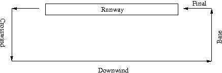
- A.10
- The rule "Approach Airport" conceptualizes the overall
purpose
of controlled approaches in a very general sense. This abstract
principle
leaves out some vital details of the actual approach procedures. To
account for one of these details, this rule was introduced. It enables
single agents to fly a basic traffic circuit, consisting of a downwind,
base, and final section. The standard traffic circuit consists
of five stages and is illustrated in the following figure:
- A.11
- For landing procedures, only downwind, base, and final are
relevant.
Although in controlled approaches the ATC decides which runway to
use, this decision is always based on the current wind direction and
velocity. The "runway in use" could be specified in field v
of figure 3.
According to this setting,
waypoints for the different approach stages were traveled by the
agents.
Internally, a manually encoded decision tree was used to generate the
agents' behavior. Since the agents were repeatedly updated based on
the chosen reset interval, an agent had to choose its next waypoint
without taking into account the previously traveled ones. The required
set of example waypoints for an approach to runway 22 left is shown
in figure 11
below. Waypoints for
the approaches to other runways were chosen accordingly.
- A.12
- Calculating the course to the next waypoint was performed similarly to the direct approach to JFK described in the above section. This rule was introduced to create a more realistic flying procedure for the agents. In the above example, an agent approaching from the north could join the traffic circuit at the final position instead of heading for the downwind point. Taking shortcuts in traffic circuits can be ordered by ATC to accelerate the flow of aircraft heading for the same runway. A desired consequence of applying this rule was to avoid head-on landings on the same runway, since this is not a realistic aspect of controlled flying. All agents were to be "funneled" through the mentioned positions, reducing the probability of simulated head-on collisions (and the probability of collisions in general). This limited concession to reality was made to investigate its impact on the general performance of the model. This rule required a specified runway to be set in field v and a coefficient in field u in the model settings (figure 3).
-
Rule "Finalize After Landing"
- A.13
- The JFK Airport was modeled as a simple cuboid with a height of 300 meters MSL. This rule provided a mechanism for the agents to switch their status to inactive after entering the JFK space. It is important to mention that real flights within the ASDI stream also disappear once the responsible ATC closes the corresponding flight plan. This usually happens shortly after landing, but the process can be delayed by more urgent concerns that require the ATC's attention.
- A.14
- One problem can arise from a late closing of real and simulated flights: An agent might stay on the runway for a long time and the corresponding real flight doing the same thing could improve the results in the statistical comparison. The comparisons should evaluate the model's performance as a model of flight approaches and not as a model of resting aircraft. To prevent palliating the statistic in this way, the "Finalize After Landing" rule was introduced. It is controlled by the checkbox q in figure 3. When switched on, this rule causes the agents to set their internal status to inactive after entering the JFK space. This automatically excludes them from all statistical comparisons.
-
The Interaction of Rules
- A.15
- A.16
- The rules interact in terms of a parallelogram of forces. Each one drives the agent according to a movement vector that results from the rule. The vectors' norm derives from the rule coefficient and is thus influenced by the genetic optimization procedure.
-
Downloading Model and Data
- A.17
- The model and all the mentioned data will be shared upon request.
![\includegraphics[width=600bp]{24_home_basti_texts_macis_svn_EPOS_jasssArticle_trafficCrw22Marked.eps}](2/trafficCrw22Marked.jpg)
![\includegraphics[scale=0.3]{15_home_basti_texts_macis_svn_EPOS_jasssArticle_halfOneOne.eps}](2/halfOneOne.jpg)
Acknowledgements
- I would like to thank several people for helping me with this paper. Elin Arbin gave linguistic advice. Nils Weidmann and Christa Deiwiks contributed helpful comments. An anonymous referee provided additional suggestions for improvement. Any remaining errors are my own.
Notes
- [1]
- The model takes the number of neighbors of an agent with the same color as a parameter x. If an agent has less than x neighbors of the same color it moves to another location. This behavior is repeated for all agents in every step.
- [2]
- Note that these screenshots were created with the Mason framework, featuring a slightly different specification of the model than proposed by Schelling (1969). For a detailed description and downloadable software, see: http://cs.gmu.edu/~eclab/projects/mason/
- [3]
- The simpler approach of performing a complete search of the
parameter
space is not practicable due to the resulting algorithmic complexity.
It is given by
 , where n is the
number of bits specifying
the parameter and k the number of parameters. Given that the parameters
are specified as integer values encoded by 32 bits, a complete search
of the configuration space for just six parameters would result in
, where n is the
number of bits specifying
the parameter and k the number of parameters. Given that the parameters
are specified as integer values encoded by 32 bits, a complete search
of the configuration space for just six parameters would result in
 necessary model runs. A heuristic
search is therefore necessary to find suitable solutions while keeping
the algorithmic complexity tractable.
necessary model runs. A heuristic
search is therefore necessary to find suitable solutions while keeping
the algorithmic complexity tractable.
- [4]
- "Federal Aviation Administration", see: http://www.faa.gov/
- [5]
- IFR stands for "Instrument Flight Rules".
- [6]
- ICAO stands for "International Civil Aviation Organization" see: http://www.icao.int/
- [7]
- ATIS stands for "automatic terminal information service" and is a radio-based service that automatically repeats weather information for international airports.
- [8]
- The website http://wunderground.com was used for this purpose.
- [9]
- All recorded data and the model will be shared upon request.
- [10]
- A formalized version of these rules can be found in the Appendix.
- [11]
- The IPH is obtainable from http://www.faa.gov/library/manuals/aviation/instrument_procedures_handbook/
- [12]
- Air tracking services such as Fboweb retrieve the Aircraft Situation Display to Industry (ASDI) data stream to provide air tracking services to their customers. This data stream contains information about the aircraft positions, orientations, altitudes and other parameters. For security reasons, the spatial resolution of this data is limited to one minute of arc (ca. 1.85 km²) and is artificially delayed for five minutes.
- [13]
- RePast is an Agent Simulation Toolkit written in Java. It can be obtained from http://repast.sourceforge.net/
- [14]
- Google Earth is a freely available software that displays a three-dimensional model of the planet textured with high resolution satellite images. It can be downloaded from http://earth.google.com/
- [15]
- A detailed description of the interaction of rules can be found in the Appendix. As a rule of thumb, one can think of the rule coefficients as a force that drives the agent into a particular direction according to the underlying rule. The resulting movement is a parallelogram of forces.
- [16]
- The collected weather information, including METARs will be shared upon request.
- [17]
- Possible STARs for JFK can be obtained online from http://www.airnav.com/airport/JFK
- [18]
- For a more elaborated analysis of this shift in paradigms, see: Cederman (1997, 3-6).
- [19]
- These formulas for Great Circle Distance and Initial Bearing were taken from http://www.movable-type.co.uk/scripts/latlong.html
- [20]
- For a grid size of one nautical mile side length, the longest possible distance is a diagonal of around 1.41 nautical miles. To travel 1.41 nautical miles per minute, a minimum ground speed of 84.6 knots or 156 km/h is required. Since the side length of the space grid fields was user-settable, a mechanism was needed to prevent agents from freezing when the grid fields were even larger.
References
- ALLEN, R.C. (1983). Collective
invention. Journal of Economic Behavior & Organization
4(1), 1-24. [doi:10.1016/0167-2681(83)90023-9]
BOERO, R. AND SQUAZZONI, F. (2005). Does Empirical Embeddedness Matter? Methodological Issues on Agent-Based Models for Analytical Social Science. Journal of Artificial Societies and Social Simulation 8(4)6 <https://www.jasss.org/8/4/6.html>
CEDERMAN, L.E. (1997). Emergent Actors in World Politics. Princeton University Press.
DEAN, J. (1966). The Pueblo Abandonment of the Tsegi Canyon, Northeastern Arizona. Paper presented at the 31st Annual Meeting of the Society for American Archeology Reno, NV, 1966.
DEAN, J. (1969). Chronological Analysis of Tsegi Phase Sites in Northeastern Arizona. Arizona University Press.
DEAN, J., EULER, R.C., GUMERMAN, G., PLOG, F., HEVLEY, R.H. AND KARSTROM, T.N.V. (1985). Human Behavior, Demography, and Palaeoenvironment on the Colorado Plateau. American Antiquity 50, 537-54, 1985. [doi:10.2307/280320]
DEAN, J., GUMERMAN, G., EPSTEIN, J.M. AND AXTELL, R.L. (2000). Understanding the Anasazi Culture Change Through Agent-Based Modeling. Dynamics of Human and Primate Societies. Oxford University Press
EPSTEIN, J.M. (2006). Generative Social Science. Princeton University Press.
EPSTEIN, J.M. AND AXTELL, R.L. (1996). Growing Artificial Societies. MIT Press.
GELLER, A. (2006). Macht, Ressourcen und Gewalt - Zur Komplexit‰t zeitgenssischer Konflikte - Eine Agentenbasierte Modellierung. vdf Hochschulverlag AG an der ETH Zrich.
GUMERMAN, G. (1988). The Anasazi in a Changing Environment. Cambridge University Press.
HAYEK, F.A. (1972). Die Theorie komplexer Ph‰nomene J. B. C. Mohr.
HEINE, B., MEYER, M. AND STRANGFELD, O. (2005). Stylised Facts and the Contribution of Simulation to the Economic Analysis of Budgeting. Journal of Artificial Societies and Social Simulation 8(4)4 <https://www.jasss.org/8/4/4.html>
PONTIUS, G. AND SCHNEIDER, L.C. (2001). Land-Cover change model validation by an ROC method for Ipswitch watershed, Massachusetts, USA. Agriculture, Ecosystems and Environments 85, 239-248. [doi:10.1016/S0167-8809(01)00187-6]
POPPER, K. (1966). Logik der Forschung. Mohr Siebeck.
KUMAR, S. AND MITRA, S. (2006). Self-Organizing Traffic at a Malfunctioning Intersection. Journal of Artificial Societies and Social Simulation vol. 9, no. 4.
SCHELLING, T.C. (1969). Models of Segregation. American Economic Review, Papers and Proceedings 59 (2): 488-493.
SHIMOKAWA, T., SUZUKI, K. AND MISAWA, T. (2007) An agent-based approach to financial stylized facts. Physica A,Volume 379, Issue 1, p. 207-225. [doi:10.1016/j.physa.2006.12.014]