Social Simulation and Analysis of the Dynamics of Criminal Hot Spots

Abstract

: Within the field of Criminology, the spatio-temporal dynamics of crime are an important subject of study. In this area, typical questions are how the behaviour of offenders, targets, and guardians can be explained and predicted, as well as the emergence and displacement of criminal hot spots. In this article we present a combination of software tools that can be used as an experimental environment to address such questions. In particular, these tools comprise an agent-based simulation model, a verification tool, and a visualisation tool. The agent-based simulation model specifically focuses on the interplay between hot spots and reputation. Using this environment, a large number of simulation runs have been performed, of which results have been formally analysed. Based on these results, we argue that the presented environment offers a valuable approach to analyse the dynamics of criminal hot spots.
Keywords:: Agent-Based Modelling, Criminal Hot Spots, Displacement, Reputation, Social Simulation, Analysis

Introduction

Criminology is an area of research that mainly addresses the analysis of criminal behaviour; e.g., (Cohen and Felson 1979; Cornish and Clarke 1986; Gottfredson and Hirschi 1990). It is a multidisciplinary area that contains elements of the Social and Behavioural Sciences, but also of disciplines like Neuroscience and, more recently, Computer Science (Lanier and Henry 1998). Although a minority of the overall population shows criminal behaviour, it typically comes in many types and variations. Within Criminology, one of the main challenges is to predict and explain in which situations which types of criminal behaviour will occur (Lanier and Henry 1998). This challenge can be addressed both from an individual (or single agent) perspective, or from a social (or multi-agent perspective). The current article focuses on the latter.

1.2

In order to explain and predict the emergence of criminal behaviour from a social perspective, several theories have been proposed within the criminological literature. Perhaps the most influential of these is the Routine Activity Theory by Cohen and Felson (1979). This (informal) theory states that three parties are relevant in the analysis of crime, i.e., offenders, targets, and guardians. More precisely, it states that a crime will occur when a motivated offender meets a suitable target and there is no guardian present.

1.3

The theory of Situational Crime Prevention is another important theory (Clarke 1980). This theory states that certain crimes can be prevented by placing guardians at appropriate locations. Such guardians may vary from police officers to alarm systems or surveillance cameras.

1.4

Theories like the Routine Activity Theory and the theory of Situational Crime Prevention have triggered a widespread attention for the interplay between the behaviour of offenders, targets, and guardians, and in particular for their spatio-temporal dynamics. For example, a relevant question is which factors influence the emergence of so-called hot spots—areas in which many crimes occur (Eck et al. 2005; Sherman et al. 1989). Based on the idea of hot spots, several related questions may be asked, among which:

when can a location in a city be defined as being a hot spot?
does the location of hot spots change over time?
does the size of hot spots change over time?
how can the emergence of hot spots be predicted?
how can the emergence of hot spots be prevented?
what is the relation between the emergence of hot spots and the geography of a city?
what is the relation between the emergence of hot spots and the demographics of the population?

1.5

In the last decades, there has been a growing interest in the area of Agent Based Social Simulation (ABSS). In ABSS, which integrates approaches from agent-based computing, computer simulation, and the social sciences, researchers try to exploit agent-based simulation to gain a deeper understanding of social phenomena (Antunes et al. 2008; Davidsson 2002). Since this approach combines the advantages of the agent paradigm (e.g., autonomy of the individual agents) with those of social simulation (e.g., the possibility to perform scalable social "experiments" without much effort), it turns out to be particularly appropriate to analyse phenomena within the criminological domain. Indeed, in recent years, a number of papers have successfully tackled criminological questions using ABSS (e.g.,Baal 2004; Brantingham and Brantingham 2004; Groff 2005; Liu and Eck 2008; Liu et al. 2005; Melo et al. 2005).

1.6

However, agent based simulation models of crime can still be improved in several ways. The role of reputation is an example of a specific aspect that has only marginally been addressed by current approaches (Brantingham and Brantingham 2004). Therefore, the current paper introduces an ABSS approach that specifically incorporates a notion of reputation of the locations involved.

1.7

The approach we propose here makes use of the high-level declarative modelling language TTL (Bosse et al. 2009) and its executable sublanguage LEADSTO (Bosse et al. 2007b). This modelling language is well suited for the current purposes, since it allows the modeller to combine qualitative, logical aspects (such as high-level agent concepts like beliefs, actions, and observations) with quantitative, numerical aspects (such as real numbers and mathematical operations). Moreover, since the language has a formal logical semantics, simulation models created in TTL and LEADSTO can be formally analysed by means of logical analysis techniques (Bosse et al. 2007a).

1.8

Below, in Section 2, some background on the concepts of reputation and displacement is provided. Next, in Section 3, the modelling languages TTL and LEADSTO are introduced. Based on this modelling approach, Section 4 describes the simulation model for the behaviour of offenders, targets, and guardians in detail. In Section 5, the simulation results are presented and in Section 6 these results are analysed using formal techniques. Section 7 discusses related work, and Section 8 concludes the paper with a discussion.

Reputation and Displacement

2.1: According to the literature in criminology, the reputation^[1] of specific locations in a city is an important factor in the spatio-temporal dynamics of crime (Herbert 1982). For example, it may be expected that the amount of assaults and the amount of arrests that take place at a certain location influence the reputation of this location. Similarly, the reputation of a location influences the attractiveness of that location for certain types of individuals. For instance, a location that is known for its high crime rates will attract police officers (Eck et al. 2005)^[2], whereas most citizens will be more likely to avoid it (Skogan 1986). As a result, the amount of criminal activity at such a location will decrease^[3], which will affect its reputation again. As can be seen from this example, the change of the reputation of locations is a highly dynamic process. Moreover, this change of reputations goes hand in hand with the change of hot spots, which is typically known as the displacement problem (Barnes 1995; Barr and Pease 1990; Cornish and Clarke 1986; Reppetto 1976).
2.2: Inspired by this displacement problem, the current paper proposes to include the notion of reputation of a location within simulation models of crime. Whereas the notion of reputation is a well-known concept in the area of Artificial Intelligence (Castelfranchi and Falcone 1998; Sabater and Sierra 2002), it is not addressed in much detail within the existing ABSS approaches to crime (e.g.Baal 2004; Brantingham and Brantingham 2004; Brantingham et al. 2005; Groff 2005; Liu and Eck 2008; Liu et al. 2005; Melo et al. 2005).
2.3: For this reason, the main objective of the current paper is to introduce an ABSS approach that incorporates the notion of reputation. In particular, the proposed approach aims at answering a specific question: how to better understand the interplay between criminal hot spots and reputation? The model can be used as an experimental tool to address this question (and related questions), by offering the possibility to predict displacement patterns under various environmental circumstances (often called "what if"-scenarios).
2.4: Typically, the input parameters of such a model are certain characteristics of the environment and the population. Examples of environmental characteristics are geographical aspects like the amount of locations, their connections, and the distances between them. Examples of characteristics of the population are the amount of agents and the ratio between offenders, targets, and guardians. Such information may or may not correspond to the characteristics of existing cities. A number of empirical criminological studies exist that try to capture such data in real cities (e.g., Bottoms and Wiles 1997). In such cases, the resulting empirical data (or an abstraction of them) may directly be used as input parameters for the simulation model. Based on this input, the output of the model shows the spatial behaviour of the different types of agents over time. Such simulation results enable the analyst to make certain predictions about the displacement of crime in a certain city, given certain circumstances.

Modelling Approach

3.1

To model the different aspects of criminal displacement from an agent perspective, an expressive modelling language is needed. On the one hand, qualitative aspects have to be addressed, such as observations, beliefs, decisions to perform an assault or an arrest, and some aspects of the environment such as the presence of certain agents. On the other hand, quantitative aspects have to be addressed. For example, the reputation of locations can best be described by a real number, and the update of this reputation can best be described by a mathematical formula. Another requirement of the chosen modelling language is its suitability to express on the one hand the basic mechanisms of criminal displacement (for the purpose of simulation), and on the other hand more global properties of criminal displacement (for the purpose of logical analysis and verification). For example, basic mechanisms of displacement of crime involve decision functions for individual agents, whereas examples of global properties are the types of statements as put forward in the introduction, like "the location of hot spots changes over time".

3.2

The predicate-logical Temporal Trace Language (TTL) (Bosse et al. 2009) fulfils all of these requirements. It integrates qualitative, logical aspects and quantitative, numerical aspects. This integration allows the modeller to exploit both logical and numerical methods for analysis and simulation. Moreover it can be used to express dynamic properties at different levels of aggregation, which makes it well suited both for simulation and logical analysis.

3.3

The TTL language is based on the assumption that dynamics can be described as an evolution of states over time. The notion of state as used here is characterised on the basis of an ontology defining a set of physical and/or mental (state) properties that do or do not hold at a certain point in time. These properties are often called state properties to distinguish them from dynamic properties that relate different states over time. A specific state is characterised by dividing the set of state properties into those that hold, and those that do not hold in the state. Examples of state properties are 'agent 1 performs an assault on agent 2', or 'there are 5 criminal agents at location A'. Real value assignments to variables are also considered as possible state property descriptions.

3.4

To formalise state properties, ontologies are specified in a (many-sorted) first order logical format: an ontology is specified as a finite set of sorts, constants within these sorts, and relations and functions over these sorts (sometimes also called signatures). The examples mentioned above then can be formalised by n-ary predicates (or proposition symbols), such as, for example, performed(assault_at(a1,a2)) or number_of_criminals(locA, 5). Such predicates are called state ground atoms (or atomic state properties). For a given ontology Ont, the propositional language signature consisting of all ground atoms based on Ont is denoted by APROP(Ont). One step further, the state properties based on a certain ontology Ont are formalised by the propositions that can be made (using conjunction, negation, disjunction, implication) from the ground atoms. Thus, an example of a formalised state property is number_of_criminals(locA, 5) & number_of_criminals(locB, 3). Moreover, a state S is an indication of which atomic state properties are true and which are false, i.e., a mapping S: APROP(Ont) → {true, false}. The set of all possible states for ontology Ont is denoted by STATES(Ont).

3.5

To describe dynamic properties of complex processes such as the displacement of crime, explicit reference is made to time and to traces. A fixed time frame T is assumed which is linearly ordered. Depending on the application, it may be dense (e.g., the real numbers) or discrete (e.g., the set of integers or natural numbers or a finite initial segment of the natural numbers). Dynamic properties can be formulated that relate a state at one point in time to a state at another point in time. A simple example is the following (informally stated) dynamic property about the number of criminals at a certain location:

For all traces γ,
there is a time point t such that
at location A, there are at least x criminal agents.

3.6

A trace γ over an ontology Ont and time frame T is a mapping γ : T → STATES(Ont), i.e., a sequence of states γt (t ∈ T) in STATES(Ont). The temporal trace language TTL is built on atoms referring to, e.g., traces, time and state properties. For example, 'in trace γ at time t property p holds' is formalised by state(γ, t) |= p. Here |= is a predicate symbol in the language, usually used in infix notation, which is comparable to the Holds-predicate in situation calculus. Dynamic properties are expressed by temporal statements built using the usual first-order logical connectives (such as ¬, ∧, ∨, ⇒) and quantification (∀ and ∃; for example, over traces, time and state properties). For example, the informally stated dynamic property introduced above is formally expressed as follows:

∀γ:TRACES ∃t:TIME ∃i:INTEGER
state(γ, t) |= number_of_criminals(locA, i) & i≥x

3.7

In addition, language abstractions by introducing new predicates as abbreviations for complex expressions are supported.

3.8

To be able to perform simulations, only part of the expressivity of TTL is needed. To this end, the executable LEADSTO language (Bosse et al. 2007b) has been defined as a sublanguage of TTL, with the specific purpose to develop simulation models in a declarative manner. In LEADSTO, direct temporal dependencies between two state properties in successive states are modelled by executable dynamic properties. The LEADSTO format is defined as follows. Let α and β be state properties as defined above. Then, the notation α →→ _{e, f, g, h} β means:

If state property α holds for a certain time interval with duration g,
then after some delay between e and f
state property β will hold for a certain time interval with duration h.

3.9

As an example, the following executable dynamic property states that "if an agent a goes to a location l during 1 time unit, then (after a delay between 0 and 0.5 time units) this agent will be at that location for 5 time units":

∀a:AGENT ∀l:LOCATION performed(a, go_to_location(l)) →→ _{0, 0.5, 1, 5} is_at_location(a, l)

3.10

Based on TTL and LEADSTO, two dedicated pieces of software have recently been developed. First, the LEADSTO Simulation Environment (Bosse et al. 2007b) takes a specification of executable dynamic properties as input, and uses this to generate simulation traces. Second, to automatically analyse the resulting simulation traces, the TTL Checker tool (Bosse et al. 2009) has been developed. This tool takes as input a formula expressed in TTL and a set of traces, and verifies automatically whether the formula holds for the traces. In case the formula does not hold, the Checker provides a counter example, i.e., a combination of variable instances for which the check fails.

3.11

For more details of the LEADSTO language and simulation environment, see (Bosse et al. 2007b). For more details on TTL and the TTL Checker tool, see (Bosse et al. 2009).

The Simulation Model

4.1

This section describes the simulation model in detail, based on the LEADSTO language. One of the main advantages of using the LEADSTO environment is that it produces simulation traces which can directly be used as input for the TTL Checker Tool. As a result, the behaviour of the model can be automatically analysed, which distinguishes this approach from related approaches in the literature (see Section 7 for an extensive comparison with related work).

4.2

The geographical aspects of the environment are modelled by a graph that consists of a number of locations, some of which are connected by edges. Within this environment, several agents move around and meet at the different locations. There are three types of agents: criminals (i.e., possible offenders), passers-by (i.e., possible targets), and guardians. The passers-by are assumed to be suitable targets, for example, because they appear rich and/or weak. However, as also the guardians are moving around, such targets may be protected, whenever at the same location a guardian is observed by the criminal (i.e., social control). Thus, a criminal agent will only perform a crime when it is at a location where it observes a passer-by and no guardians. An example of a simple geographical environment is shown in Figure 1. This picture represents a small city that only consists of three important locations (called A, B, and C), and is populated by 30 agents. The black circles denote passers-by, the grey circles denote guardians, and the white circles denote criminals. As can be seen in the figure, in this situation crimes may be performed at location B, since this location contains 1 criminal, 4 passers-by, and no guardians.

4.3

The interaction between a specific agent and the environment is modelled by (1) observation, which takes information on the environment as input for the agent (e.g., at which location it is, where suitable targets are, and whether social control is present), and (2) performing actions, which is an output of the agent affecting the state of the world (e.g., going to a different location, or committing a crime).

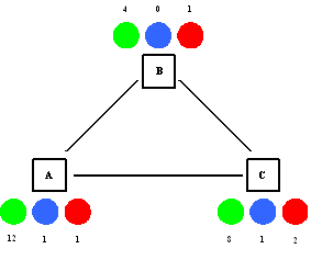
Figure 1. Example geographical environment
This figure shows three locations, called A, B and C. The locations are connected to each other. The green circles depict the number of passers-by present at that location, the blue circles depict the guardians and the red circles depict the number of criminals.

4.4

In order to decide to which location they will go, all agents continuously update the attractiveness (or utility) they assign to each location, which is represented by a real number in the domain [0,1]. This attractiveness is calculated as the weighted sum of three values (also represented by real numbers), namely:

The individual basic attractiveness v the agent assigns to that location. This represents the extent to which the agent likes to go to that location, independent of its reputation. For example, some agents are more likely to go to a shopping centre, whereas others are more likely to go to a railway station.
The assault reputation n1 of the location. The higher this number, the more famous the corresponding location is for assaults taking place there.
The arrest reputation n2 of the location. The higher this number, the more famous the corresponding location is for arrests taking place there.

4.5

This calculation is represented by the following executable dynamic property (in LEADSTO format):

Decide Current Location Attractiveness
∀a:AGENT ∀l:LOCATION ∀n1,n2,v,w1:REAL ∀w2,w3:INTEGER
basic_attractiveness_of_agent_for_location(v, l, a) ∧
belief(a, assault_reputation_at_location(n1, l)) ∧
belief(a, arrest_reputation_at_location(n2, l)) ∧ has_weight_factor(a, w1, w2, w3)  →→ 
belief(a, current_attractiveness_of_location(l, w1 × v+w2 × n1+w3 × n2))

As can be seen from this rule, each agent possesses three individual weight factors w1, w2, and w3, which indicate the relative importance they attach to each of the three components introduced above. Note that these weight factors may be positive or negative. For instance, criminals will usually have a positive weight factor for assault reputation (they will tend to go to locations where many assaults have been performed in the past, since they expect that their chances to perform a next assault are higher at those locations), and a negative weight factor for arrest reputation (they will tend to avoid locations where many arrests have been performed in the past). Similarly, passers-by will usually have a very negative weight factor for assault reputation and a negative weight factor for arrest reputation. Finally, guardians will usually have a very positive weight factor for assault reputation and a positive weight factor for arrest reputation.

4.6

Based on the calculated attractiveness of the locations, each agent determines where to go, by selecting the location with the highest attractiveness.

4.7

By integrating the idea of utility-based, multi-criteria decision making with the notion of reputation, the model basically combines two distinct mechanisms for decision making^[4]. On the one hand, the function to calculate attractiveness is inspired by the logic of rational-choice theory and forward-looking utility maximising (cf. Tsebelis 1989; 1990). This means that agents seek to optimise their locations, in particular that criminals will look for low detection probabilities, guardians for high detection probabilities and passers-by for low assault probabilities. On the other hand, the notion of reputation reflects the logic of learning and backward-looking decision-making models (cf. Macy and Flache 2002). This implies that agents learn from the observation of other agents' behaviour. As a consequence, agents are assumed to copy successful behavior of agents with the same characteristic, i.e. criminals copy successful behavior of other criminals, guardians copy successful behavior of other guardians and passers-by copy successful behavior of other passers-by (where the copying refers to the choice of the location).

4.8

According to Brantingham and Brantingham (1984), daily life patterns of offenders might also influence the location of offending behaviour, even when the offender is engaging, to some degree, in a search pattern for a suitable target, having already decided to commit an offence. They argue that offenders are more likely to perform an assault in a neighbourhood they know well. They are more likely to avoid neighbourhoods that they are not familiar with. In the simulation model presented here, such differences in preferences for certain locations can be expressed by means of the basic attractiveness predicate.

4.9

Next, as mentioned above, the criminal agents decide to perform an assault when they are at a location where they observe a passer-by and no guardians, cf. the Routine Activity Theory (Cohen and Felson 1979). This is modelled by the following dynamic property:

Perform Assault
∀a1,a2:AGENT ∀l:LOCATION
observes(a1, agent_of_type_at_location(a1, criminal, l)) ∧
observes(a1, agent_of_type_at_location(a2, passer_by, l)) ∧
not guardian_at_location(l)  →→ 
performed(a1, assault_at(a2, l))

4.10

After having performed an assault, a criminal becomes a known criminal for a number of time steps. This is done to ensure that the guardians are able to recognise (and possibly arrest) a criminal that performed a crime. In the simulation runs described in the next section, criminals stay "known" for 4 iterations, which represents a period during which they are actually being wanted by the police. After such a period, these criminals become anonymous again. However, when a guardian meets a criminal that is still wanted, (s)he will arrest that criminal. This is modelled by the following dynamic property:

Perform Arrest
∀a1,a2:AGENT ∀l:LOCATION
observes(a1, agent_of_type_at_location(a1, guardian, l)) ∧
observes(a1, agent_of_type_at_location(a2, criminal, l)) ∧
known_criminal(a2)  →→ 
performed(a1, arrest_at(a2, l))

4.11

Furthermore, the assault reputation of the different locations involved is increased each time that an assault is performed, cf. the following dynamic property:

Assault Reputation Increment
∀l:LOCATION ∀n:REAL
assault_at(l) ∧ 
belief(all_agents, assault_reputation_at_location(n, l))  →→ 
belief(all_agents, assault_reputation_at_location(n+inc, l))

Here, inc is a constant that specifies the increment of reputation based on one assault. In the simulation runs described in the next section, inc = 1. Note that this dynamic property assumes that all agents have the same knowledge about reputations. By replacing all_agents by a variable for a specific agent, variants of this rule can be created for different agents.

4.12

When no assault is performed at a location, the reputation of this location for being a hot spot slightly decreases:

Assault Reputation Decay
∀l:LOCATION ∀n:REAL
belief(all_agents, assault_reputation_at_location(n, l)) ∧
not assault_at(l)  →→ 
belief(all_agents, assault_reputation_at_location(n × dec, l))

Here, dec is a constant that specifies the decay of reputation when there is no assault. In the simulation runs described in the next section, dec = 0.99.

4.13

To update the arrest reputation of locations, the same rules are used as shown above, where the word assault is replaced by arrest.

4.14

Finally, it is assumed that the (assault and arrest) reputation of all locations is known to all agents in the population (e.g., because events like assaults and arrests are publicly discussed in the media, or because they are communicated between agents). However, the approach could be made more realistic by replacing the reputation mechanism by specific trust update mechanisms for individual agents (cf. Castelfranchi and Falcone 1998).

4.15

The complete set of LEADSTO rules used for the simulation model (including the time parameters) is shown in Appendix A.

Simulation Results

5.1

The simulation model as described in the previous section has been used to generate various simulation traces under different parameter settings. This section describes an example of a simulation trace in detail. In the next section, the global results of all simulation runs are summarised and discussed.

5.2

The parameter settings used for the simulation described in this section are identical to the ones shown in Figure 1: the population consists of 24 passers-by, 2 guardians and 4 criminals. Initially, these agents are distributed over the locations by means of their personal preferences (i.e., the basic_attractiveness predicates). Moreover, weight factors are assigned to each agent. The details of these parameter settings can be found in Appendix B.

5.3

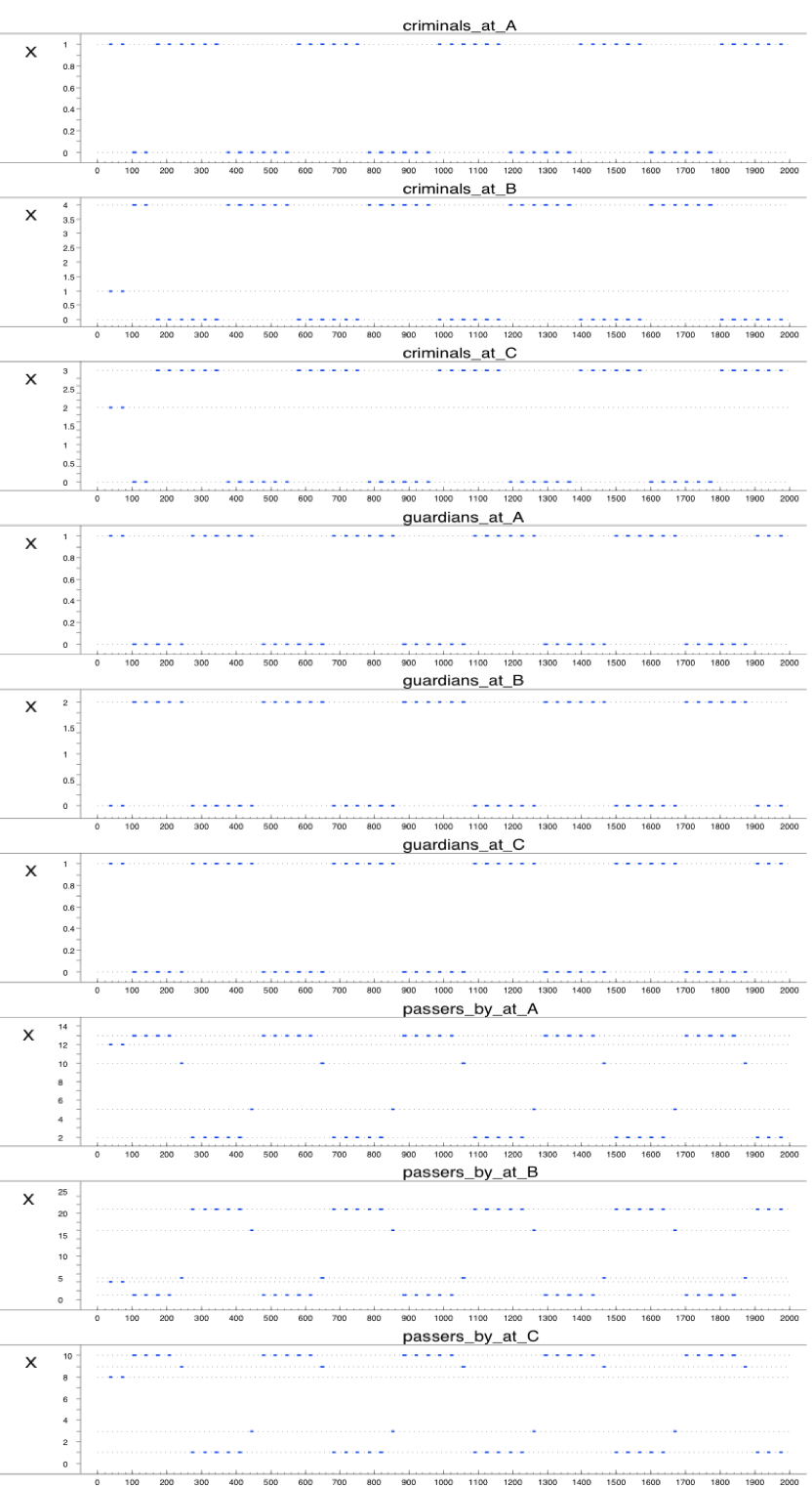
Part of the simulation trace that was generated using these settings is shown in Figure 2 (A-C). Within these graphs, time is on the horizontal axis (where each geometric shape indicates a new iteration of movements), and the number of agents at a certain location is at the vertical axis. As shown in Figure 2B (and also in Figure 1), initially there are no guardians at location B. As a result, some assaults take place at that location. This leads to a change in the assault reputation of that location, which eventually results in displacement. This can be seen in the third iteration (around time point 100): most of the passers-by move away from location B (although one of them still remains at that location), whereas all criminals and all guardians move towards location B. As a result of this, some arrests take place, which leads to a change in arrest reputation of location B. As a consequence, again, the criminals move (in the fifth iteration, around time point 160), this time to location A and C. Since location A and C are now populated by criminals and passers-by, but not by guardians, some assaults take place at that location, which again leads to a change in assault reputation, and in displacement of the passers-by and the guardians. This cycle repeats itself until the end of the simulation: the passers-by move away from the criminals (and if possible, towards the guardians), the criminals follow the passers-by (as long as they do not encounter too many guardians), and the guardians follow the criminals. However, it is important to note that there is no strict sequential order in these movements (in the sense that one of the groups would always move 'earlier' or 'faster' than the others). In fact, Figure 2 shows that in the third iteration, all groups move simultaneously (namely, the passers-by move away from location B whereas the other two groups move towards location B). However, the result of these movements is that a new situation emerges, in which apparently the criminals are least satisfied, since they are the 'first' to decide to move again (in the fifth iteration), whereas the other two groups decide to stay. This leads again to a new situation, in which the passers-by decide to move (in the seventh iteration), followed by the guardians (in the eighth iteration), and so on.

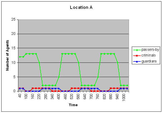
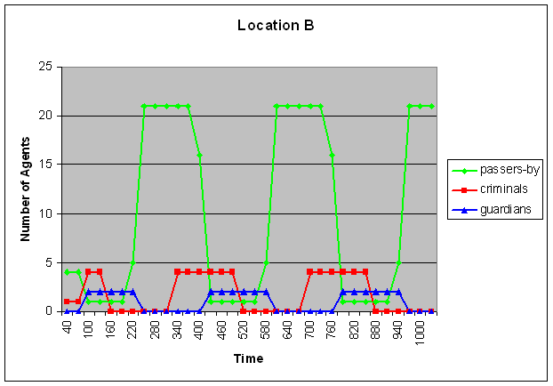
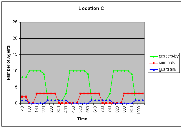
Figure 2. Displacement of the three types of criminals
Here time is on the horizontal axis and the number of agents is depicted on the vertical axis. The upper graph represents location A, the middle graph location B and the graph below represents location C. The green line shows the amount of passers-by, the red line the amount of criminals and the blue line the amount of guardians.

5.4

To understand the influence of assaults on the assault reputation, see Figure 3, which depicts the dynamics of the assault reputation of location A. Note that, as opposed to Figure 2, this picture is a screenshot of the LEADSTO simulation environment. As shown in Figure 3, whenever an assault is performed, the assault reputation of this location immediately increases. However, when no assaults are performed, the assault reputation gradually decreases. For example, at time point 160, 190, and 220, location A contains a criminal and several passers-by, but no guardians (see Figure 2A). As a result, assaults are performed, which increases the assault reputation of that location (after a small delay), as shown in Figure 3. This figure also shows the gradual decay of the assault reputation in between these three assaults.

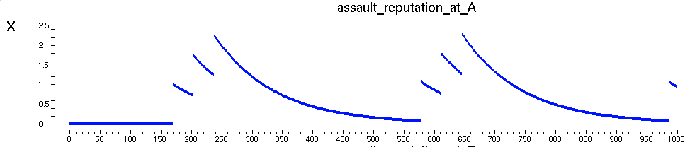
Figure 3. Assault reputation of location A
This figure shows an immediate increase after a crime has been committed. When no crimes are committed, the assault reputation decreases gradually due to decay.

5.5

A similar trend can be observed in Figure 4, which depicts the dynamics of the arrest reputation of location A. The dynamics of the reputations of the other locations are not shown. However, these show similar behaviour as depicted in Figure 3 and 4.

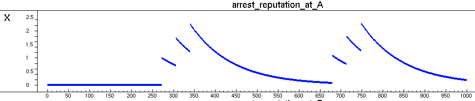
Figure 4. The arrest reputation of location A
This figure shows a similar pattern as the assault reputation. After an arrest the reputation of the location increases quite rapidly. When no arrest is performed on that location, the reputation decreases gradually.

Visualisation of Simulation Runs

5.6

To provide the user more insight in the exact (spatial) dynamics of a simulation trace, a visualisation tool has been developed in Matlab. The tool takes an arbitrary simulation trace as input and generates an animation of the crime dynamics (which can be stored as .mpg-files). In Figure 5, a screenshot of such an animation is shown. Here, each intersection represents a location in a city. Note that this example is unrelated to the scenario addressed above. In the example addressed here, instead of 3, there are now 25 locations in total that are connected through edges (according to a grid or 'block' structure). However, the numbers of agents are still the same (i.e., 24 passers-by, 4 criminals, and 2 guardians). The different agents can meet each other at the intersections. The green dots denote passers-by, the blue dots are guardians and the red dots are criminals. In addition, the black dots represent the reputation of a certain location. The bigger the dot, the higher the assault reputation of that location.

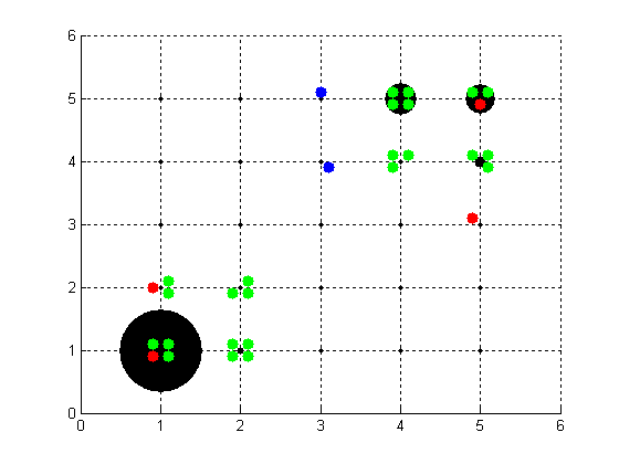
Figure 5. Screenshot of the Visualisation Tool. In this figure, twenty-five locations are depicted (i.e., the intersections of the dotted lines). Here the blue dots represent the guardians, the red dots the criminals and the green dots the passers-by. The black dots represent the reputation of a certain location

Formal Analysis

6.1

All in all, a large series of simulation runs has been performed. The detailed settings and results of a simple example of these simulations (i.e., the one described in Section 5.1) are shown in Appendix B. Among the different simulations, various parameter settings were varied, in particular the number of agents, the ratio between different types of agents, the number of locations, the basic attractiveness of locations for the agents, and the weight factors of the agents.

6.2

To analyse the resulting simulation traces in more detail, the TTL Checker tool (Bosse et al. 2009) has been used. As mentioned earlier, this tool takes as input a TTL formula and a set of traces, and verifies automatically whether the formula holds for the traces. For the current domain, a number of hypotheses have been expressed as dynamic properties in TTL, which were inspired by the questions mentioned in the Introduction. For example, consider the following dynamic property (P1), which expresses that the location of hot spots keeps on changing over time:

6.3

P1 Continuation of Displacement For each time point t (except the end of the trace^[5]), if at t the largest hot spot is at location x, then there is a later time point at which the largest hot spot is at some other location y.

∀γ:TRACES ∀t:TIME ∀x:LOCATION
[ is_largest_hot_spot_at(x, t, γ) & t  <  last_time - δ ]
⇒ [ ∃t2:TIME ∃y:LOCATION is_largest_hot_spot_at(y, t2, γ) &
      t < t2 & x≠y]

6.4

In this formula, is_largest_hot_spot_at is an abbreviation, which can be determined in multiple ways. For example, by taking the location: 1) with the highest assault reputation, 2) with the highest number of criminals, or 3) with the highest number of crimes. These different possibilities are formalised as follows:

is_largest_hot_spot_at(x,t,γ) ≡
∃r:REAL state(γ, t) |= assault_reputation(x, r) &
∀y:LOCATION ∀r2:REAL
   [state(γ, t) |= assault_reputation(y, r2) ⇒ r2 ≤ r ]

is_largest_hot_spot_at(x,t,γ) ≡
∃i:INTEGER state(γ, t) |= number_of_criminals(x, i) &
∀y:LOCATION ∀i2:INTEGER
   [state(γ, t) |= number_of_criminals(y, i2) ⇒ i2 ≤ i ]

is_largest_hot_spot_at(x,t,γ) ≡
∃i:INTEGER state(γ, t) |= number_of_crimes(x, i) &
∀y:LOCATION ∀i2:INTEGER
   [state(γ, t) |= number_of_crimes(y, i2) ⇒ i2 ≤ i ]

6.5

In addition, a combination of the different options can be considered, for example, by calculating the weighted sum of the different numbers. Yet another variant of the dynamic property can be created, for example, by counting the number of criminals or crimes over a longer time period, instead of considering the current time point only.

6.6

Note that the term hot spot is used in many different ways by researchers and police. Although no common definition of the term hot spot of crime exists, the common understanding is that a hot spot is an area that has a greater than average number of criminal or disorder events, or an area where people have a higher than average risk of victimisation. Hot spot analysis can be performed on multiple levels, e.g., on the level of addresses, blocks, or regions (Eck et al. 2005). This variability in definition is reflected in our approach by the possibility to choose one out of multiple formulae, as shown above.

6.7

Besides checking whether the location of hot spots is continuously changing, also other properties can be verified. A relevant property from the viewpoint of crime prevention is to check whether specific reoccurring patterns can be identified. For example, is it always the case that the criminals follow the movement of the passers-by, and that the guardians follow the criminals? And if not, are there specific circumstances in which this pattern does not occur? To analyse these kinds of patterns, properties like the following have been established:

6.8

P2a Criminals follow Passers-by For each time point t (except the end of the trace), if at t most passers-by are at location x, then within ε time points most criminals will be at location x.

∀γ:TRACES ∀t:TIME ∀x:LOCATION
[most_passers_by_at(x, t, γ) & t  <  last_time - δ ]
⇒ [ ∃t2:TIME most_criminals_at(x, t2, γ) & t < t2 & t2 < t+ε]

Here, most_passers_by_at is defined as follows:

most_passers_by_at(x,t,γ) ≡
∃i:INTEGER state(γ, t) |= number_of_passers_by(x, i) &
∀y:LOCATION ∀i2:INTEGER
   [state(γ, t) |= number_of_passers_by(y, i2) ⇒ i2 ≤ i ]

Similarly, most_criminals_at is defined by taking the location with the highest number of criminals (see the second formalisation of is_largest_hot_spot_at above). In addition to P2a, a similar property has been created to check whether the guardians follow the criminals:

6.9

P2b Guardians follow Criminals For each time point t (except the end of the trace), if at t most criminals are at location x, then within ε time points most guardians will be at location x.

∀γ:TRACES ∀t:TIME ∀x:LOCATION
[most_criminals_at(x, t, γ) & t  <  last_time - δ ]
⇒ [ ∃t2:TIME most_guardians_at(x, t2, γ) & t < t2 & t2 ≤ t+ε]

Here, obviously, most_criminals_at is defined as follows:

most_criminals_at(x,t,γ) ≡
∃i:INTEGER state(γ, t) |= number_of_criminals(x, i) &
∀y:LOCATION ∀i2:INTEGER   [state(γ, t) |= number_of_criminals(y, i2) ⇒ i2 ≤ i ]

6.10

A third property has been established to check whether there are any periods during a simulation in which agents spread (more of less) equally over the different locations. This may be an indication that the presence of hot spots has (temporarily) disappeared. For example, for criminals, this can be checked via the following property:

6.11

P3(Criminals)—Equal spread of criminals over locations There are time points t1 and t2 such that for all time points in between, and for all locations x, the amount of criminals at x is within a range of δ of the total amount of criminals c divided by the number of locations NL.

∃t1,t2:TIME ∀t3:TIME ∀x:location ∀i:real
   [t1 < t3 < t2 & state(γ, t3) |= number_of_criminals(x, i)  ⇒ c/NL = i ± c × δ]

In the trace shown in Figure 2, this property clearly does not hold, since at every point in time some locations are more attractive than other locations.

6.12

Finally, a number of properties have been specified to investigate the relation between the emergence of hot spots and the number of locations, and the relation between the emergence of hot spots and the ratio between the types of agents. For example, the following formula can be used to check the property that 'more locations lead to less crime':

6.13

P4—More locations lead to less crime For all traces γ1 and γ2, if there are more locations in γ1 than in γ2, then at the end of the simulation there will be less crime in γ1.

∀γ1, γ2:TRACES ∀x1,x2,i1,i2:INTEGER
 state(γ1, te) |= total_number_of_locations(x1) &
 state(γ2, te) |= total_number_of_locations(x2) &
 state(γ1, te) |= total_number_of_crimes(i1) &
 state(γ1, te) |= total_number_of_crimes(i2) &
x1 > x2   ⇒ i1  <  i2

6.14

Here, te denotes the last time point of the simulation. Moreover, the predicate total_number_of_crimes is defined by summation of the crimes over all locations and all time points. Note that this property usually will not hold. However, in addition to simply checking whether the property holds, the TTL checking tool also allows the modeller to check how often it holds, i.e., in which percentage of the cases, and in which specific situations it does not hold. Such checks may provide the researcher important information about the relation between the geography of a city and the emergence of hot spots.

6.15

All in all, the above properties have been checked against a large number of simulation traces under different parameter settings (see also the appendix mentioned in Bosse and Gerritsen (2008)). The results pointed out that in almost all of the simulations, the same repeating pattern was found: the passers-by move away from the criminals, the criminals follow the passers-by, and the guardians follow the criminals. We therefore conclude that the pattern is quite robust to variations in parameter settings, which is an encouraging result, since the pattern is similar to the trends described in criminological literature (Barr and Pease 1990; Cornish and Clarke 1986; Reppetto 1976), and game-theoretical literature on crime and control such as Rauhut (2009). Intuitively, this finding makes sense, since the three groups involved have fundamentally conflicting interests (e.g., passers-by want to escape criminals, whilst criminals want to catch passers-by). In the game theoretical literature, this situation is referred to as 'discoordination situation' and is known to produce cycles due to the non-existence of Nash equilibria in pure strategies. In addition, the model has similarities with the classical Lotka-Volterra models (also known as predator-prey models, cf. Morin 1999), which show similar cyclical behaviour (although they typically involve two groups instead of three).

6.16

Only in some exceptional cases, this cyclical pattern was not found. For example, when there are more guardians then locations, the guardians may distribute themselves over the locations, so that no crime will ever be performed, and thus no displacement will occur. This case may be compared with the ideal situation that a city has sufficient police force to prevent all crime. Another exception was a situation in which many agents have extreme preferences. For instance, if a certain location has an extremely high attractiveness to passers-by, then these passers-by will stay at that location, even though they run the risk of being assaulted.

Related Work

7.1: The part of criminology concerned with the displacement of crime is called environmental criminology. Within this area the key object is the study of crime, criminality, and victimization as they relate to particular places and to the way that individuals and organisations shape their activities spatially (Bottoms and Wiles, 1997; Bottoms 2007). Among the main research groups within this area is the Chicago School of Sociology. Shaw and McKay, two researchers from this school, made an important contribution in the early 1940s (Shaw and McKay 1942). They found that delinquency rates were at their highest in inner-city zones and decreased the further one moved out of the city and into the suburbs. Further, they indentified that this spatial patterning of juvenile crime remained stable irrespective of the neighborhood's racial or national demographic composition (McLaughlin and Muncie 2001; Shaw and McKay 1942). The work of Shaw and McKay concentrated mainly on area offender rates. After that, the focus shifted towards the rediscovery of the offence and later on the explaining of offender rates. Recently, crime mapping is one of the important topics within the field of environmental criminology, especially by means of computerised geographical information systems (GIS). These systems can act as the means of linking together any types of data which are capable of being geo-coded (Bottoms and Wiles, 1997). The main difference with the approach proposed in this paper is that GIS record empirical crime data as they are, and use these for visualisation or analysis. Instead, our approach attempts to make predictions of crime-related patterns over time (possibly, but not necessarily, inspired by empirical data; see the discussion section).
7.2: Besides the literature in Criminology, also in Artificial Intelligence a number of modelling approaches exist that have similarities to the approach discussed in this paper. This section is not meant to provide a complete overview (see Liu and Eck 2008 for that purpose), but will discuss those approaches that, to our knowledge, are most related to the current paper.
7.3: To start, the work in Groff (2005) systematically investigates the geography of crime trajectories using a variety of spatial analysis techniques. However, a difference with the current approach is that these models do not contain an adaptive element (such as an update of reputation), which causes the results to converge quickly to an equilibrium.
7.4: Another approach to analyse the spatio-temporal dynamics of crime is presented in Brantingham et al. (2005). This approach is based on a Distributed Abstract State Machine (DASM) formalism, combined with a multi-agent based modelling paradigm. Although the agents involved are capable of learning (using a form of behavioural reinforcement learning, where based on past experiences certain preferences are developed that may influence future choices), the notion of reputation is not explicitly incorporated.
7.5: A third interesting approach is introduced in Liu et al. (2005), which also explores the possibility of simulating individual crime events in order to generate plausible crime patterns. This approach is based on a Cellular Automaton (CA), in which the main elements are offenders, targets, and crime places. Different attributes of the model can be manipulated, among which motivation of offenders, capability of guardians, and accessibility of places. Like the approach mentioned above, the main difference with the current approach is that it does not contain an explicit notion of reputation.
7.6: Furthermore, a more specialised approach is presented in Melo et al. (2005). That paper describes a tool to investigate the influence that different police control routes have on the reduction of crime rates. The approach comprises an artificial society consisting of various agents, in particular criminals and policemen. As a follow-up of that work, in Reis et al. (2006) the first results are presented that were achieved with GAPatrol, an evolutionary multi agent-based simulation tool devised to assist police managers in the design of effective police patrol route strategies.
7.7: Another more specialised approach is put forward in Baal (2004). This approach specifically aims at simulating the process of deterrence. A simulation model is presented where each potential offender is part of a social network that consists of several agents. All agents repeatedly face a choice between rule compliance and rule transgression. If agents transgress, they have a probability of being audited and punished. The main aim of the work is to investigate how the probability of being punished influences the amount of crime.
7.8: Although all of the papers mentioned above have some similarities with the work presented here, an important difference is that they all focus on simulation only. In contrast, the current paper proposes an approach that combines simulation with logical analysis. Since the simulation traces that result from the LEADSTO environment can directly be used as input for the TTL Checker, it is relatively easy for the modeller to verify certain global properties of the model. As such, the paper has many similarities with the work presented in Bosse et al. (2007a), which also combines simulation with logical analysis. However, the domain addressed by the latter paper is completely different (namely the psychological and biological characteristics underlying the behaviour of criminals that are diagnosed with "Intermittent Explosive Disorder"). In addition, that paper does not consider the notion of reputation, nor does it address any notion of adaptivity.

Discussion

8.1: Within the area of Criminology, analysis of the spatio-temporal dynamics of crime is an important challenge. In particular, criminologists are interested in the question where criminal hot spot may emerge, and when they will emerge. As a first step towards answering such questions, the current paper presents an agent-based simulation model that can be used as an experimental tool to analyse spatio-temporal dynamics of crime. The simulation model particularly focuses on the interplay between hot spots and reputation, which has not been addressed in earlier work.
8.2: As usual in Agent-Based Social Simulation, the model has been set up in a generic manner, according to the principles of compositionality and knowledge abstraction (Brazier et al. 2000). This means that, when one wants to study another scenario (i.e., analyse the behaviour of another city, or population), the complete behavioural specification of the system (see Appendix A) can be re-used. All that needs to be filled in is a number of domain specific slots, e.g., concerning the geographical environment, or the initial distribution of agents.
8.3: Using the model, a series of simulation runs has been performed, under different parameter settings. The results of the simulations have been automatically verified (by means of the TTL Checker,Bosse et al. 2009) against a number of hypotheses, expressed as logical formulae. In almost all of the simulations, the same repeating pattern was found: the passers-by move away from the criminals, the criminals follow the passers-by, and the guardians follow the criminals. Although there is no overall agreement in the criminological literature about an exact definition of displacement (see, e.g.,Reppetto 1976), this pattern is quite similar to the displacement trends described by authors such as Barr and Pease (1990) and Cornish and Clarke (1986).
8.4: In fact, one could argue that this is a rather unsatisfactory finding, since it may lead to the conclusion that "the police always arrive too late" (or, more concretely, that decisions to establish new patrol teams, surveillance cameras, and so on, are only made after the hot spots have already emerged). Therefore, an interesting question, which we are currently focussing on, is whether simulation models of criminal displacement can be useful for anticipatory policies (i.e., to increase the number of guardians at locations where hot spots are likely to emerge, instead of at the present locations of hot spots). The first results of a extensive comparison between a number of strategies (varying from merely reactive to more anticipatory) which we are currently performing show that anticipatory strategies indeed seem to lead to less crime than reactive strategies (Bosse and Gerritsen 2009).
8.5: Furthermore, note that, although the parameter settings used for the simulations described in this paper were inspired by empirical studies such as Bottoms and Wiles (1997)^[6], no effort was put into creating settings that correspond exactly to the characteristics of real cities and populations. Therefore, the results of the presented simulations should not be considered as conclusive about real world situations. Rather, they provide preliminary insight in the process of displacement, and provide support for the usefulness of the presented approach as an analysis tool. As shown in Section 5 and 6, the presented combination of software tools (i.e., the LEADSTO simulation tool, the TTL Checker tool, and the Matlab visualisation tool) can be very useful for the researcher to study criminal displacement. In particular, the LEADSTO simulation tool can be used to generate large numbers of traces under different parameter settings. Next, the TTL Checker tool can be used to filter out those traces for which unexpected behaviour occurs. After that, these particular traces can be studied in more detail using the Matlab visualisation tool, in order to explain the unexpected behaviour.
8.6: The intended users of these tools are in the first place researchers in criminology, although on the long term they may be also useful for policy makers. When one considers the intended users of similar tools that have been proposed in the literature (Baal 2004; Brantingham et al. 2005; Groff 2005; Liu et al. 2005; Melo et al. 2005; Reis et al. 2006), it turns out that different perspectives are taken. For example, some authors have attempted to develop simulation models of crime displacement in existing cities, which can be directly related to real world data (e.g.,Liu et al. 2005), whereas others deliberately abstract from empirical information (e.g.,Bosse et al. 2008). The idea behind the latter perspective is that the simulation environment is used as an analytical tool, mainly used by researchers and policy makers, to shed more light on the process under investigation, and perhaps improve existing policies (e.g., for surveillance) on the long run (Elffers and Baal 2008). The point of view taken in the current paper can be situated in between these two extremes. Initially, the simulation model was developed to study the phenomenon of displacement per se. However, its basic concepts have been defined in such a way that they can be directly connected to empirical information, if this becomes available. Indeed, the authors also plan to use more realistic parameter settings in the future (including temporal relationships), in order to investigate to what extent the approach is able to reproduce empirical data. As soon as the model can be sufficiently validated in such settings (i.e., the global patterns produced by the model match the empirical data), the model may be of interest for policy makers, e.g. to study 'what-if' scenarios. For example, one may investigate how the crime level of a certain city will change if the policy makers invest in more surveillance in a certain area.
8.7: When such more realistic parameter settings will be considered, also scaling issues will have to be addressed. Although the current simulation model handles population sizes of hundreds of (heterogeneous) agents relatively easily, the simulation time is polynomial in the number of agents. Therefore, complexity problems will arise when populations of (more than) thousands of agents are considered. These problems could be solved by translating the current simulation model to a stochastic model, as is done, for example, in the analysis of epidemics (Anderson and Britton 2000). Also for the displacement of criminal hot spots, such a translation is currently being made. An initial version of such a stochastic model of criminal displacement (where the behaviour of the different agent types was kept simple) is presented in Bosse et al. (Bosse 2008). When making such a translation, the description of the dynamics of a population shifts from a "micro" perspective (at the level of individual agents) to a "macro" perspective (at the level of groups of agents). For example, the number of criminals, assaults and arrests at certain locations can be described by global variables, which are influenced by probabilistic rules. A comparable, but slightly different approach is presented in Bosse et al. (2007a), where the expected number of crimes in certain populations is estimated on the basis of probabilities of opportunities. The main advantage of these types of macro-level approaches is that they can deal with larger populations. An inevitable drawback is however that they imply a loss of detail at the individual agent level. In current work in progress, the benefits of such approaches are explored in more detail.
8.8: Concerning other future work, various extensions to the model will be considered. An interesting expansion could be based on the work by Sampson et al. (1997). They state that the social cohesion of a group is an important factor in the emergence of crime. Social cohesion among neighbours combined with their willingness to intervene on behalf of the common good, is linked to reduced violence. An interesting direction for further research would be to introduce a parameter for social cohesion, in order to investigate whether that increases the accuracy of the simulation model.

Appendix A—LEADSTO Specification

A.1: Below, the complete specification of the criminal displacement model is shown, in LEADSTO notation. Note that the LEADSTO simulation software can be downloaded from the following URL: http://www.cs.vu.nl/~wai/TTL/.
Decide Current Location Attractiveness ∀a:AGENT ∀l:LOCATION ∀n1,n2,v,w1:REAL ∀w2,w3:INTEGER basic_attractiveness_of_agent_for_location(v, l, a) ∧ belief(a, assault_reputation_at_location(n1, l)) ∧ belief(a, arrest_reputation_at_location(n2, l)) ∧ has_weight_factor(a, w1, w2, w3) ∧ agents_counted →→ _{0, 0, 1, 1} belief(a, current_attractiveness_of_location(l, w1 × v+w2 × n1+w3 × n2)) Go to Most Attractive Location ∀a:AGENT ∀l1,l2,l3:LOCATION ∀x1,x2,x3:REAL belief(a, current_attractiveness_of_location(l1, x1)) ∧ belief(a, current_attractiveness_of_location(l2, x2)) ∧ belief(a, current_attractiveness_of_location(l3, x3)) ∧ l1≠l2 ∧ l2≠l3 ∧ l1≠l3 ∧ x1>x2 ∧ x1>x3 →→ _{0, 0, 1, 1} performed(a, go_to_location(l1)) Arrive at Location ∀a:AGENT ∀l:LOCATION performed(a, go_to_location(l)) →→ _{0, 0, 1, nr_agents+4} is_at_location(a, l) Observe all Agents ∀a:AGENT ∀l:LOCATION ∀r:INTEGER ∀t:TYPE is_at_location(a, l) ∧ has_type(a, t) ∧ round(r) →→ _{0, 0, nr_agents+1, 1} observes(a, agent_of_type_at_location(a, t, l)) Count Types of Agents at Locations ∀a:AGENT ∀l:LOCATION performed(a, go_to_location(a, t, l)) →→ _{0, 0, 1, 1} counting_at(1) ∧ agents_counted_of_type_at_location(0, passer_by, locA) ∧ agents_counted_of_type_at_location(0, passer_by, locB) ∧ agents_counted_of_type_at_location(0, passer_by, locC) ∧ agents_counted_of_type_at_location(0, criminal, locA) ∧ agents_counted_of_type_at_location(0, criminal, locB) ∧ agents_counted_of_type_at_location(0, criminal, locC) ∧ agents_counted_of_type_at_location(0, guardian, locA) ∧ agents_counted_of_type_at_location(0, guardian, locB) ∧ agents_counted_of_type_at_location(0, guardian, locC) ∀k:between(0, nr_agents) ∀l:LOCATION ∀n:between(1, nr_agents+1) ∀t:TYPE counting_at(n) ∧ n ≤ nr_agents agents_counted_of_type_at_location(k, t, l) ∧ is_at_location(agent(n), l) ∧ has_type(agent(n), t) →→ _{0, 0, 1, 1} agents_counted_of_type_at_location(k+1, t, l) ∧ counting_at(n+1) ∀k:between(0, nr_agents) ∀l,l2:LOCATION ∀n:between(1, nr_agents+1) ∀t:TYPE counting_at(n) ∧ n ≤ nr_agents ∧ agents_counted_of_type_at_location(k, t, l) ∧ is_at_location(agent(n), l2) ∧ l≠l2 ∧ has_type(agent(n), t) →→ _{0, 0, 1, 1} agents_counted_of_type_at_location(k, t, l) ∧ counting_at(n+1) ∀k:between(0, nr_agents) ∀l,l2:LOCATION ∀n:between(1, nr_agents+1) ∀t,t2:TYPE counting_at(n) ∧ n ≤ nr_agents ∧ agents_counted_of_type_at_location(k, t, l) ∧ is_at_location(agent(n), l2) ∧ t≠t2 ∧ has_type(agent(n), t2) →→ _{0, 0, 1, 1} agents_counted_of_type_at_location(k, t, l) ∧ counting_at(n+1) Believe Counted Types of Agents ∀k:between(0, nr_agents) ∀l:LOCATION ∀n:between(1, nr_agents+1) ∀t:TYPE counting_at(n) ∧ n > nr_agents ∧ agents_counted_of_type_at_location(k, t, l) →→ _{0, 0, 1, 1} belief(all_agents, number_of_type_at_location(k, t, l)) ∧ agents_counted Note: all_agents is an abbreviation for a conjunction of all the agents in the simulation. Visualise Counted Types of Agents ∀k:between(0, nr_agents) ∀l:LOCATION ∀t:TYPE belief(all_agents, number_of_type_at_location(k, t, l)) →→ _{0, 0, 1, 10} visualise_agents_of_type_at_location(k, t, l) Perform Assault ∀a:AGENT ∀l:LOCATION is_at_location(a, l) ∧ has_type(a, guardian) →→ _{0, 0, 1, 1} guardian_at_location(l) ∀a1,a2:AGENT ∀l:LOCATION observes(a1, agent_of_type_at_location(a1, criminal, l)) ∧ observes(a1, agent_of_type_at_location(a2, passer_by, l)) ∧ not guardian_at_location(l) →→ _{0, 0, 1, 1} performed(a1, assault_at(a2, l)) Count Assaults ∀a1,a2:AGENT ∀l:LOCATION performed(a1, assault_at(a2, l)) →→ _{0, 0, 1, 1} assault_at(l) ∀l:LOCATION ∀a:AGENT ∀n:REAL assault_at(l) ∧ belief(a, assault_reputation_at_location(n, l)) →→ _{0, 0, 1, 1>} belief(a, assault_reputation_at_location(n+inc, l)) ∀l:LOCATION ∀a:AGENT ∀n:REAL belief(a, assault_reputation_at_location(n, l)) ∧ not assault_at(l) →→ _{0, 0, 1, 1} belief(a, assault_reputation_at_location(n*dec, l)) Perform Arrest ∀a1,a2:AGENT ∀l:LOCATION performed(a1, assault_at(a2, l)) →→ _{0, 0, 1, nr_agents × 4} known_criminal(a1) ∀a1,a2:AGENT ∀l:LOCATION observes(a1, agent_of_type_at_location(a1, guardian, l)) ∧ observes(a1, agent_of_type_at_location(a2, criminal, l)) ∧ known_criminal(a2) →→ _{0, 0, 1, 1} performed(a1, arrest_at(a2, l)) Count Arrests ∀a1,a2:AGENT ∀l:LOCATION performed(a1, arrest_at(a2, l)) →→ _{0, 0, 1, 1} arrest_at(l) ∀l:LOCATION ∀a:AGENT ∀n:REAL arrest_at(l) ∧ belief(a, arrest_reputation_at_location(n, l)) →→ _{0, 0, 1, 1} belief(a, arrest_reputation_at_location(n+inc, l)) ∀l:LOCATION ∀a:AGENT ∀n:REAL belief(a, arrest_reputation_at_location(n, l)) ∧ not arrest_at(l) →→ _{0, 0, 1, 1} belief(a, arrest_reputation_at_location(n × dec, l)) Maintain Rounds - needed for observations ∀r:INTEGER round(r) →→ _{3, 3, nr_agents+1, nr_agents+1} round(r+1)

Appendix B—Simulation 1

A.2

In this section, an example simulation run is shown. For the sake of readability, a simple case of three locations is chosen.

A.3

First, the simulation settings are shown, in the table below. The first column indicates the name of the agent, the second column indicates the type of agent (criminal, guardian, or passer-by), the next three columns indicate the basic attractiveness of that agent for the different locations (A, B, and C), the next three columns indicate the three weight factors of that agent (w1, w2, and w3), and the last column indicates the initial location of the agent.


Agent	Type	A	B	C	W1	W2	W3	Start
1	PB	0.87	0.81	0.74	0.1	0	0	A
2	PB	0.81	0.76	0.70	0.1	-1	0	A
3	PB	0.83	0.74	0.68	0.1	-2	-1	A
4	PB	0.77	0.60	0.51	0.1	-3	-2	A
5	PB	0.79	0.64	0.58	0.1	-4	-3	A
6	PB	0.85	0.60	0.66	0.1	-5	-4	A
7	PB	0.83	0.59	0.61	0.5	0	0	A
8	PB	0.84	0.63	0.70	0.5	-1	0	A
9	PB	0.89	0.66	0.72	0.5	-2	-1	A
10	PB	0.81	0.43	0.52	0.5	-3	-2	A
11	PB	0.86	0.51	0.62	0.5	-4	-3	A
12	PB	0.90	0.52	0.71	0.5	-5	-4	A
13	PB	0.81	0.90	0.74	1.1	0	0	B
14	PB	0.76	0.84	0.51	1.1	-1	0	B
15	PB	0.53	0.76	0.68	1.1	-2	-1	B
16	PB	0.60	0.81	0.76	1.1	-3	-2	B
17	PB	0.76	0.64	0.83	1.1	-4	-3	C
18	PB	0.78	0.61	0.81	1.1	-5	-4	C
19	PB	0.79	0.70	0.84	2.1	0	0	C
20	PB	0.70	0.63	0.76	2.1	-1	0	C
21	PB	0.81	0.75	0.90	0.1	-2	-1	C
22	PB	0.74	0.68	0.79	0.5	-3	-2	C
23	PB	0.60	0.79	0.85	1.1	-4	-3	C
24	PB	0.74	0.80	0.86	2.1	-5	-4	C
25	G	0.85	0.74	0.79	0.1	4	3	A
26	G	0.81	0.76	0.83	0.1	5	4	C
27	C	0.84	0.81	0.80	0.1	2	-3	A
28	C	0.76	0.86	0.84	1.1	3	-4	B
29	C	0.78	0.81	0.83	1.1	3	-5	C
30	C	0.83	0.82	0.85	2.1	4	-5	C

A.4

In this simulation, there are 24 passers by, 2 guardians and 4 criminals in the world. As shown in the resulting trace, initially, they are distributed over the location by means of their personal preferences (i.e., a predicate that states which location they find most attractive/interesting). At time point 100, there are 13 passers by at location A and there are 10 passers by at location C. At time point 160, the criminals go after the passers by. There is 1 criminal at location A and 3 criminals went to location C. This results in the movement of passers by. They want to move away from the criminals and they go to location B (time point 260). Only 100 time points later, the criminals follow the passers by and they also arrive at location B (time point 360). The passers by want to get away from the criminals and return to the locations A and C. Again 100 time points later, the criminals also move to location A and C (respectively 1 and 3 criminals). This trend repeats itself until the end of the trace. The guardians follow the criminals. They arrive at the location of the criminals 100 time points after the criminals do.

Acknowledgements

: A shorter, preliminary version of this paper appeared in: Proceedings of the Seventh International Joint Conference on Autonomous Agents and Multi-Agent Systems, AAMAS'08. ACM Press, 2008. The authors are grateful to Henk Elffers and Jan Treur for very fruitful discussions about the topic. Further, we would like to thank the anonymous reviewers for their time and their useful remarks.

Notes

¹In this paper, the concept of reputation is studied as a characteristic of a location (or geographical area). More specifically, the reputation of a location is defined as a (publicly known) measure for the amount of crime-related activities (e.g. assaults or arrests) that take place, which is built up on the basis of past events (involving multiple individuals) at that location. Note that this definition differs from the idea of reputation as a characteristic of an individual, as often used in the literature. For an overview of the different notions of reputation in different disciplines (including Evolutionary Biology, Economy, and Computer Science), see Mui et al. (2000).

²Note that this is an over-simplification of police deployment practices. Police officers are indeed more attracted to places with high crime rates, but this is usually part of larger actions against crime. An example is the Street Crime Initiative in the UK (Home Office 2003). This is an initiative taken by five police forces which together accounted for 72% of all street robberies and actually targeted the ten police force areas where street crime levels were highest. Over 30 different projects were designed to tackle the street crime problem from different angles. Youth work, environmental planning, increased surveillance, reducing market of stolen goods, and targeted enforcement are just a number of possible interventions (Home Office 2003). For practical purposes, in our model we decided to simplify such interventions by simply assuming that criminals attract (both formal and informal) guardians.

³Although a location's reputation is an important factor in the process of displacement, it is not the only factor that determines the movement of offenders, targets, and guardians. Also various other aspects of a location may play a role in attracting or repelling certain groups (e.g., escape routes, abandoned buildings, possibilities to buy drugs, and so on). These concepts are modelled in Section 4 by means of the basic_attractiveness predicate.

⁴For a comprehensive review of the differences between forward- and backward-looking decision making models with respect to crime and control (including empirical evidence), see Rauhut (2009).

⁵the condition t < last_time-δ (where δ is the maximum duration of displacement, for example 6 iterations) was added to make sure that the property does not fail for the end of the trace.

⁶For example, the authors tried to pick reasonably realistic settings for agents' preferences and ratios between types of agents.

References

ANDERSON, H., and Britton, T. (2000). Stochastic Epidemic Models and Their Statistical Analysis. Springer-Verlag, NY. [doi:10.1007/978-1-4612-1158-7]

ANTUNES, L., Paolucci, M., and Norton, E. (eds) (2008). Multi-Agent-Based Simulation VIII-LNAI 5003. Berlin: Springer. [doi:10.1007/978-3-540-70916-9]

BAAL, P.H.M. van (2004). Computer Simulations of Criminal Deterrence: from Public Policy to Local Interaction to Individual Behaviour. Ph.D. Thesis, Erasmus University Rotterdam. Boom Juridische Uitgevers.

BARNES, G.C. (1995). Defining and Optimizing Displacement. In: Eck, J.E. and Weisburd, D. (eds.), Crime and Place (Monsey, NY: Criminal Justice Press and Washington, DC: Police Executive Research Forum), pp. 95-113.

BARR, R., and Pease, K. (1990). Crime Placement, Displacement and Deflection. In: Tonry, M. and Morris, M. (eds.), Crime and Justice: A Review of Research, vol. 12. Chicago: University of Chicago Press, pp. 277-315. [doi:10.1086/449167]

BOSSE, T. and Gerritsen, C. (2008). Agent-Based Simulation of the Spatial Dynamics of Crime: on the interplay between criminals hot spots and reputation. In: Proceedings of the Seventh International Joint Conference on Autonomous Agents and Multi-Agent Systems, AAMAS'08, ACM Press, pp. 1129-1136, 2008.

BOSSE, T. and Gerritsen, C. (2009). Comparing Crime Prevention Strategies by Agent-Based Simulation. In: Proceedings of the 9th IEEE/WIC/ACM International Conference on Intelligent Agent Technology, IAT'09. IEEE Computer Society Press, 2009, to appear. [doi:10.1109/wi-iat.2009.200]

BOSSE, T., Gerritsen, C., Hoogendoorn, M., Jaffry, S.W., and Treur, J. (2008). Comparison of Agent-Based and Population-Based Simulations of Displacement of Crime. In: Jain, L., Gini, M., Faltings, B.B., Terano, T., Zhang, C., Cercone, N., and Cao, L. (eds.), Proceedings of the Eighth IEEE/WIC/ACM International Conference on Intelligent Agent Technology, IAT'08. IEEE Computer Society Press, 2008, pp. 469-476. [doi:10.1109/wiiat.2008.333]

BOSSE, T., Gerritsen, C., and Treur, J. (2007a). Cognitive and Social Simulation of Criminal Behaviour: the Intermittent Explosive Disorder Case. In: Proceedings of the Sixth International Joint Conference on Autonomous Agents and Multi-Agent Systems, AAMAS'07. ACM Press, pp. 367-374. [doi:10.1145/1329125.1329195]

BOSSE, T., Jonker, C.M., Meij, L. van der, Sharpanskykh, A., and Treur, J., (2009). Specification and Verification of Dynamics in Agent Models. In: International Journal of Cooperative Information Systems, vol. 18, 2009, pp. 167-193. [doi:10.1142/s0218843009001987]

BOSSE, T., Jonker, C.M., Meij, L. van der, and Treur, J. (2007b). A Language and Environment for Analysis of Dynamics by SimulaTiOn. In: Journal of AI Tools, vol. 16, issue 3, 2007, pp. 435-464. [doi:10.1142/S0218213007003357]

BOTTOMS, A.E., and Wiles, P. (1997). Environmental Criminology. In: Maguire, M., Morgan, R., and Reiner, R. (eds.), The Oxford Handbook of Criminology. Oxford: Oxford University Press, pp. 620-656.

BOTTOMS, A. E. (2007). Place, Space, Crime and Disorder. In: Maguire, M., Morgan, R., and Reiner, R. (eds.), The Oxford Handbook of Criminology. Oxford Univerisity Press, pp. 528-574.

BRANTINGHAM, P. and Brantingham, P. (1984). Patterns in crime. New York: Macmillan.

BRANTINGHAM, P. L., and Brantingham, P. J. (2004). Computer Simulation as a Tool for Environmental Criminologists. Security Journal, 17(1), 21-30. [doi:10.1057/palgrave.sj.8340159]

BRANTINGHAM, P.L., Glässer, U., Singh, K., and Vajihollahi, M. (2005). Mastermind: Modeling and Simulation of Criminal Activity in Urban Environments. Technical Report SFU-CMPTTR-2005-01, Simon Fraser University.

BRAZIER, F.M.T., Jonker, C.M., and Treur, J. (2000). Compositional Design and Reuse of a Generic Agent Model. Applied Artificial Intelligence Journal, vol. 14, 2000, pp. 491-538. [doi:10.1080/088395100403397]

CASTELFRANCHI, C., and Falcone, R. (1998). Principles of Trust for MAS: Cognitive Anatomy, Social Importance, and Quantification. In: Demazeau, Y. (ed.), Proceedings of the Third International Conference on Multi-Agent Systems, ICMAS'98, IEEE Computer Society, Los Alamitos, pp. 72-79. [doi:10.1109/icmas.1998.699034]

CLARKE, R.V.G. (1980). "Situational" Crime Prevention: theory and practice. British Journal of Criminology, vol.20 pp. 136-147.

COHEN, L.E., and Felson, M. (1979). Social change and crime rate trends: a routine activity approach. American Sociological Review, vol. 44, pp. 588-608. [doi:10.2307/2094589]

CORNISH, D.B., and Clarke, R.V. (1986). Situational prevention, displacement of crime and Rational Choice Theory. In: Heal, K. and Laycock, G. (eds.), Situational crime prevention: from theory to practice, London: HMSO, pp. 1-16.

CORNISH, D.B., and Clarke, R.V. (1986). The Reasoning Criminal: Rational Choice Perspectives on Offending. Springer Verlag. [doi:10.1007/978-1-4613-8625-4]

DAVIDSSON, P. (2002). Agent Based Social Simulation: A Computer Science View. Journal of Artificial Societies and Social Simulation, 5(1).

ECK, J. E., Chainey, S., Cameron, J. G., Leitner, M., and Wilson, R. E.. (2005). Mapping crime: Understanding hot spots. National Institute of Justice, U.S. Department of Justice, 2005. URL: http://www.ojp.usdoj.gov/nij/pubs-sum/209393.htm.

ELFFERS, H., and Baal, P. van. (2008). Spatial Backcloth is not that important in simulation research: An illustration from simulating perceptual deterrence. In: L. Liu and J.E. Eck (eds.), Artificial crime analysis systems, pp. 19-34. Hershey, PA: IGI Global. [doi:10.4018/978-1-59904-591-7.ch002]

GOTTFREDSON, M., and Hirschi, T. (1990). A General Theory of Crime. Stanford University Press.

GROFF, E.R. (2005). The Geography of Juvenile Crime Place Trajectories. Ph.D. Thesis: University of Maryland.

HERBERT, D.T. (1982). The Geography of Urban Crime. Longman: Harlow, England.

HOME Office United Kingdom (2003). Streets Ahead: A Joint Inspection of the Street Crime Initiative. Home Office Communication Directorate.

LANIER, M.M. and Henry, S., (1998). Essential Criminology. Westview Press: Boulder, Colorado.

LIU, L., and Eck, J., (eds.) (2008). Artificial Crime Analysis Systems: Using Computer Simulations and Geographic Information Systems. Information Science Reference. [doi:10.4018/978-1-59904-591-7]

LIU, L., Wang, X., Eck, J., and Liang, J. (2005). Simulating Crime Events and Crime Patterns in RA/CA Model. In F. Wang (ed.), Geographic Information Systems and Crime Analysis. Singapore: Idea Group, pp. 197-213. [doi:10.4018/978-1-59140-453-8.ch012]

MACY, M.W. and Flache, A. (2002), Learning Dynamics in Social Dilemmas. In: Proceedings of the National Academy of Sciences, vol. 99, pp. 7229-7236. [doi:10.1073/pnas.092080099]

MCLAUGHLIN, E. and Muncie, J. (2001). The Sage Dictionary of Criminology. Sage: London.

MELO, A., Belchior, M., and Furtado, V. (2005). Analyzing Police Patrol Routes by Simulating the Physical Reorganisation of Agents. In: Sichman, J.S., and Antunes, L. (eds.), Multi-Agent-Based Simulation VI, Proceedings of the Sixth International Workshop on Multi-Agent-Based Simulation, MABS'05. Lecture Notes in Artificial Intelligence, vol. 3891, Springer Verlag, 2006, pp 99-114.

MORIN, P.J. (1999). Community Ecology. Blackwell Publishing, USA.

MUI, L., Halberstadt, A., and Mohtashemi, M. (2000). Notions of reputation in multi-agent systems: A review. In: Proceedings of the First International Conference on Autonomous Agents, AAMAS'02. ACM Press, pp. 280-287.

RAUHUT, H. (2009). Higher punishment, less control? Experimental evidence on the inspection game. Rationality and Society, vol. 21, issue 3. [doi:10.1177/1043463109337876]

REIS, D., Melo, A., Coelho, A.L.V., and Furtado, V. (2006). Towards Optimal Police Patrol Routes with Genetic Algorithms. In: Mehrotra, S., et al. (eds.), ISI 2006. LNCS 3975, pp. 485-491. [doi:10.1007/11760146_45]

REPPETTO, T.A. (1976). Crime Prevention and the Displacement Phenomenon. Crime & Delinquency, vol. 22, pp. 166-177. [doi:10.1177/001112877602200204]

SABATER, J. and Sierra, C. (2002) Reputation and social network analysis in multi-agent systems. In: Proceedings of the First International Conference on Autonomous Agents, AAMAS'02. ACM Press, pp. 475-482. [doi:10.1145/544741.544854]

SAMPSON, R.J., Raudenbush, S.W., and Earls, F. (1997). Neighborhoods and violent crime: A multilevel study of collective efficacy. Science, vol. 277, pp. 918-924. [doi:10.1126/science.277.5328.918]

SHAW, C. and McKay, H. (1942). Juvenile Delinquency and Urban Areas. University of Chicago Press, Chicago.

SHERMAN, L.W., Gartin, P.R., and Buerger, M.E. (1989). Hot Spots of Predatory Crime: Routine Activities and the Criminology of Place. Criminology, vol. 27, pp. 27-55. [doi:10.1111/j.1745-9125.1989.tb00862.x]

SKOGAN, W. (1986). Fear of crime and neighborhood change. In: Reiss, A. J., Jr., and Tonry, M. (eds.), Communites and Crime (Crime and Justice, vol. 8), University of Chicago Press, Chicago, pp. 203-229. [doi:10.1086/449123]

TSEBELIS, G. (1989). The Abuse of Probability in Political Analysis: The Robinson Crusoe Fallacy. American Political Science Review, vol. 83, issue 1, pp. 77-91. [doi:10.2307/1956435]

TSEBELIS, G. (1990). Penalty has no impact on crime. A game-theoretic analysis. Rationality and Society, vol. 2, issue 3, pp. 255-286. [doi:10.1177/1043463190002003002]

Hide
Article Tools

Smaller Text Bigger

Bookmark:

Export citation

Articles with the same author(s)

Articles with similar keywords

Articles citing this article

Download this article in PDF format

Alert me when this article is cited within JASSS

Send a link to this article to a colleague