
 Abstract
- The spatial distribution of crime has been a long-standing interest in the field of criminology. Research in this area has shown that activity nodes and travel paths are key components that help to define patterns of offending. Little research, however, has considered the influence of activity nodes on the spatial distribution of crimes in crime neutral areas - those where crimes are more haphazardly dispersed. Further, a review of the literature has revealed a lack of research in determining the relative strength of attraction that different types of activity nodes possess based on characteristics of criminal events in their immediate surrounds. In this paper we use offenders' home locations and the locations of their crimes to define directional and distance parameters. Using these parameters we apply mathematical structures to define rules by which different models may behave to investigate the influence of activity nodes on the spatial distribution of crimes in crime neutral areas. The findings suggest an increasing likelihood of crime as a function of geometric angle and distance from an offender's home location to the site of the criminal event. Implications of the results are discussed.
- Keywords:
- Crime Attractor, Directionality of Crime, Mathematical Modeling, Computational Criminology
Introduction
- 1.1
-
Investigating the spatial distribution of crime across geographic
areas has been a long-standing interest of scholars, sociologists,
and criminologists over the past two centuries (Burgess 1925). More
recently, criminologists have advanced our knowledge in this area by
demonstrating that crime is not randomly distributed, rather it
exhibits clear spatial patterns. Specifically, the geometric theory
of crime informs us that activity nodes and travel paths are key
components that help to define such patterns (Brantingham and Brantingham 1981). Nodes and
paths shape the activity and awareness spaces of individuals which
contribute to the target selection behaviour of potential offenders
and ultimately determine where crimes may occur. With this research,
the role of activity nodes (in this case suburban regional shopping
centres) on criminal activity is investigated.
- 1.2
-
The concentration of crime at place has been well established in
criminological literature. For example, a sizable body of research
has shown that crimes tend to cluster at certain geographic
locations (see for example, Sherman et al. (1989)). Crime generators and crime attractors
(Brantingham and Brantingham 1995) are two types of areas where crimes tend to
concentrate. Crime generators draw masses of people who without any
predetermined criminal motivation stumble upon an opportunity too
good to pass up. Crime attractors lure motivated offenders because
of known criminal opportunities. Only a relatively small amount of
research, however, has considered the influence of activity nodes on
the spatial patterning of crime neutral areas (Brantingham and Brantingham 1995) - those
where crimes are more sporadically distributed with few clusters or
concentrations. Despite the seemingly haphazard spread of crimes in
these areas, the tenets of Crime Pattern Theory
suggest that an underlying pattern should be present. Since the
target selection behaviours of criminals are influenced by their
awareness spaces which are largely defined by nodes and
paths in their daily travel routines, it is expected that crimes will be
committed along the routes between offenders' homes and activity
node locations (Brantingham and Brantingham 1993). In order to
understand the attraction of activity nodes and uncover the
systematic distribution of crimes in the crime neutral areas around
them, a mathematical structure is needed to model components that
contribute to patterns of crime.
Patterns of Human Activity
- 2.1
-
Many factors influence how an individual navigates in an urban area,
including their personal mobility, transportation options, and the
physical form of the city. Geographic theories are used to describe
the patterns of activity of urban residents including those from
behaviourial geography which examines, at its core, the connections between spatial decision-making, human cognition,
and human movements in the environment (see Argent and Walmsley (2009) and
Golledge et al. (2001)). Lynch's seminal work (1960), The Image of the
City, was one of the first to examine an individual's perception of
space as applied to navigation through urban areas. The author
argued that individuals understand and therefore navigate through
their surroundings in predictable ways. They do this by using
'mental maps' with five basic elements: paths (roads, transit
lines), edges (walls, boundaries, shorelines), districts (defined
areas, neighbourhoods), nodes (urban focal points such as railway
stations, intersections, or plazas), and landmarks (physical
structure unique in its environs). A person maneuvering their way
through an urban area utilizes their knowledge of these spatial
elements in order to successfully carry out all of their daily
activities such as shopping, recreation, or the daily commute back
and forth from work.
- 2.2
-
Individuals interact with their surrounding environments in
predictable ways. Activity space is a key concept in
human-environment interaction studies, defined as the set of
locations that an individual has direct contact with as a result of
the execution of their daily activities (Golledge and Stimson 1997). Core
geographic principles are at the heart of the activity space idea,
including distance decay, referring to the decreasing likelihood of
interaction as a function of distance, and directional bias, an
agent's predisposition to move in a particular direction at the
expense of other directions (Rai et al. 2007). These concepts help to
describe the differential likelihood of people interacting with
other individuals or environments. The characteristics (size, shape)
of a person's activity space are likely to be determined by home
residence location (urban, suburban, rural), socio-economic status
(SES) (Morency et al. 2009), age and gender (see Matthews (1980) and Mercado and Pimez (2009)), and
personal mobility (Kopec 1995) in addition to many other potential
determinants. The activity space concept has been widely applied,
owing to its utility and flexibility for modeling the socio-spatial
context of diverse urban phenomena. It has been utilized for this
purpose in a variety of disciplines including geography, public
health, transportation studies, and criminology (see for example, Mason and Korpela (2009)).
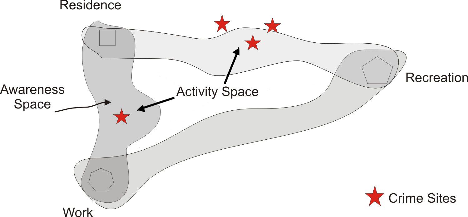
- 2.3
-
It is likely that a person has knowledge of environments beyond
their usual activity space. All places that an individual has some
knowledge of constitutes their awareness space (Brown et al. 1977).
Knowledge of places outside of one's activity space is likely to
exist according to the principle of distance decay, wherein a person
will have greater awareness of places geographically proximal to
their activity space. For an example, see Figure 1.
Patterns of Crime
- 3.1
-
The criminological sub-field of environmental criminology uses the
concepts discussed above to understand criminal activity in the
context of urban environments. The target selection behaviour of
offenders is one area of research within this sub-field that has
generated considerable interest. A variety of factors including the
attractiveness and accessibility of an area, and the opportunities
available within an area have been found to influence where
offenders commit crimes (Bernasco and Luykx 2003). These patterns even exist for
different age-groups (Groff 2005). The theoretical foundation that
informs the design of the proposed model is the geometric theory of
crime (Brantingham and Brantingham 1981). The central idea divulged from this framework is
that crime locations are largely dependent upon where potential
offenders reside and what their awareness spaces consist of, and
where potential targets are located and whether they are located
within an offender's awareness space3. In short, while the target selection behaviour of
offenders has been shown to be influenced by a variety of factors
related to the characteristics of areas, criminal event locations
are ultimately bound by the activity and awareness spaces of
potential offenders.
- 3.2
-
There are several factors that contribute to defining a person's
activity and awareness spaces. Nodes and paths are two concepts that
are of greatest concern for the purposes of the current discussion.
In general, people move from one activity to the next, spending time
at several locations throughout the day. Home, work, school,
shopping centres, entertainment venues and recreation sites are
common activity nodes that consume the majority of our daily lives.
Since some activity nodes draw larger masses of people (e.g.,
shopping centres and sports stadiums), they are said to have a
greater pull or attraction. In contrast, some activity nodes draw
fewer people (e.g., single family dwellings and stand-alone
commercial properties) and are said to have a reduced pull or
attraction. Several criminological studies have demonstrated the
pull of specific types of activity nodes based on their
concentrations of crime and the spatial-temporal transitions of
certain crime types (see Kinney et al. (2008) and Bromley and Nelson (2002)). In Bromley and Nelson (2002), for
example, the authors found that hot spots of alcohol related crimes
in Worcester exhibited clear spatial-temporal transitions. Pubs and
clubs attracted high concentrations of alcohol related crime around
midnight but this type of crime shifted after the alcohol outlets
closed. In the early morning hours alcohol related crimes
concentrated closer to residential areas.
Overview of Journey to Crime Research
- 3.3
-
Paths are the spaces used to navigate between activity nodes.
Roadways and walkways are two examples of paths that connect us from
one place to the next. Since individuals develop routine travel
patterns to and from their destinations, paths contribute to the
activity and awareness spaces that define an offender's target
search area. The importance of travel paths has also been
demonstrated in criminological literature (see Bromley and Nelson (2002) and Alston (1994)).
In Alston's (1994) study of target selection patterns of
serial rapists, for example, initial contact with victims was
repeatedly found to be near routine travel paths. Related to the
target selection behaviours of potential offenders are components
of an offender's journey to crime. Three elements that constitute an
offender's journey to crime include a starting location (usually an
offender's home location), the direction of travel, and the distance
from starting point to crime location (Rengert 2004). To date, journey
to crime research has largely been dominated by investigations into
the distance factor. Generally, it has been found that most crimes
occur short distances from offenders' home locations and follow a
distance decay pattern (Wiles and Costello 2000).
- 3.4
-
According to literature (Brantingham and Brantingham 1995), crimes can be separated
into two general categories, probably should read "those against a specific property, which are usually tied to a location, or those against a person,
which are usually not tied to fixed locations. In this paper the
focus is on those crimes where the location plays a central role,
hence the application of the model is restricted in this paper to
only property-crimes.
Extending Journey to Crime to Directionality
- 3.5
-
The directionality component of an offender's journey to crime is
largely determined by the configuration of their activity nodes and
travel paths. If most of their activities fall along a single
trajectory, directionality should be strong. While research on this
topic is quite sparse, there is some evidence that suggests activity
nodes do influence the directionality of crimes because of their
general forces of attraction. In Rengert and Wasilchick (1985) for example, the
authors investigated offenders' directional preferences in burglary
offences. They found a strong directional preference towards
offenders' places of employment. In fact, most of the offences were located just past the offenders' work locations or along the travel paths between home and work. Public transport systems are also
influential in the development of offenders' awareness spaces.
Transit systems in urban areas transport people across great
distances along a limited number of paths and to a limited number of
transit hubs. As a result, awareness spaces can become tightly
clustered (Brantingham et al. 1991).
- 3.6
-
There are still many questions about the influence of activity nodes
that remain unanswered. It is unknown, for example, whether the
spatial patterning of crimes in crime-neutral areas can be described
by the relationship between the directionality of offenders'
movements and activity nodes. We are also unaware of any research
that has investigated the relative strength of attraction that
different types of activity nodes possess based on characteristics
of criminal events in their immediate surrounds.
- 3.7
-
Mathematical modeling has been applied in several social science
research initiatives. Recent applications in the field of
criminology have included agent based, cellular automata, process,
and system dynamics models (see for example, Brantingham and Tita (2008), Dabbaghian et al. (2010), Li (2008), Alimadad et. al. (2008), Gerritsen (2010) and Malleson and Brantingham (2008)). These types of
models focus on the actual movement of agents (offenders), their
interaction with the environment, and the development of patterns
while assuming an underlying set of rules for the model. The current
project differs from these previous approaches by applying
mathematical structures to define the actual rules by which the above
mentioned models may behave. Using directional and distance
parameters defined by offenders' home locations and the locations of
their crimes, the influence of activity nodes on the spatial
distribution of crimes in crime neutral areas is investigated.
Study Area
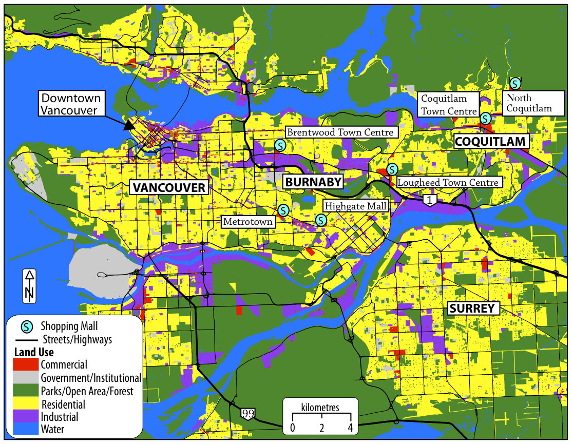
- 4.1
-
The sites of investigation for this study were Burnaby and
Coquitlam; two fast-growing suburban cities in the Metro Vancouver
region located in the extreme south-west of British Columbia,
Canada. This urban region consists of 22 municipalities with a total
population of 2,275,000 (BCStats 2009), see Figure 2.
- 4.2
-
The City of Burnaby, located immediately to the east of the City of
Vancouver (620,000 residents), is the third largest of the 22
municipalities by population with approximately 220,000 residents.
The city is effectively split in two by Highway 1, resulting in
distinct north and south areas of the city. Due to its suburban
relation to Vancouver proper, residential land uses have
traditionally dominated in Burnaby, including a mix of apartments
and single-detached housing types. Burnaby has gradually become more urban in recent years however, as industrial and commercial
land-uses have increasingly proliferated. Commercial land-use in
Burnaby includes the Metrotown neighbourhood in South Burnaby which
boasts the largest shopping centre in British Columbia: Metropolis
at Metrotown (simply called Metrotown hereafter). Other large
shopping centres include Lougheed Town Centre and Brentwood Town
Centre, both located in North Burnaby. In South Burnaby there were
1250 criminal events for 1037 offenders, while in North Burnaby
there were 521 criminal events for 466 offenders.
- 4.3
-
The City of Coquitlam—with a residential population of
approximately 125,000—is located to the east of Burnaby in the
Metro Vancouver region. Land-use in Coquitlam is primarily
single-family residential, as it primarily functions as a bedroom
community for Vancouver and surrounding areas. There is some
industrial and commercial activity in Coquitlam, less however than
in neighbouring Burnaby. The main commercial area in Coquitlam is Coquitlam Town Centre, a centrally-located retail destination that
also includes a high-rise residential neighbourhood. Average family
income in 2005 was $74,413 for Burnaby and $82,934 for Coquitlam,
both below the metropolitan area average of $87,788 (BCStats 2006).
In Coquitlam, for this study, there were 20493 criminal offenses for
16920 offenders.
- 4.4
-
As a result of collaboration between the Institute of Canadian Urban
Research Studies (ICURS) research center at the School of
Criminology at SFU and the Royal Canadian Mounted Police (RCMP),
five years of real-world crime data was made available for research
purposes at ICURS. This data was retrieved from the RCMP's Police
Information Retrieval System (PIRS). PIRS contains the type of calls
for service for the entire division of RCMP in British Columbia (BC)
between August 1, 2001 and August 1, 2006. It records all calls, and
contains data about the subjects (people), as well as vehicles and
businesses involved in the event and what their involvement was. All
property crime and offender home locations for the cities which are
analyzed in this paper were extracted from this dataset. For those
offenders with a valid home or crime location, the locations were
geocoded onto the road-network to get longitudes and latitudes. The
home location is kept in its original form as it was reported by the
offender to the police at the time of the offense (which could be a
friend's house, home or shelter). The crime location was where the
crime event actually occurred. The data geocoded at a rate of 90%,
which exceeds the minimum standard of 85% identified by
Ratcliffe (2004). If any location did not geocode, it was discarded.
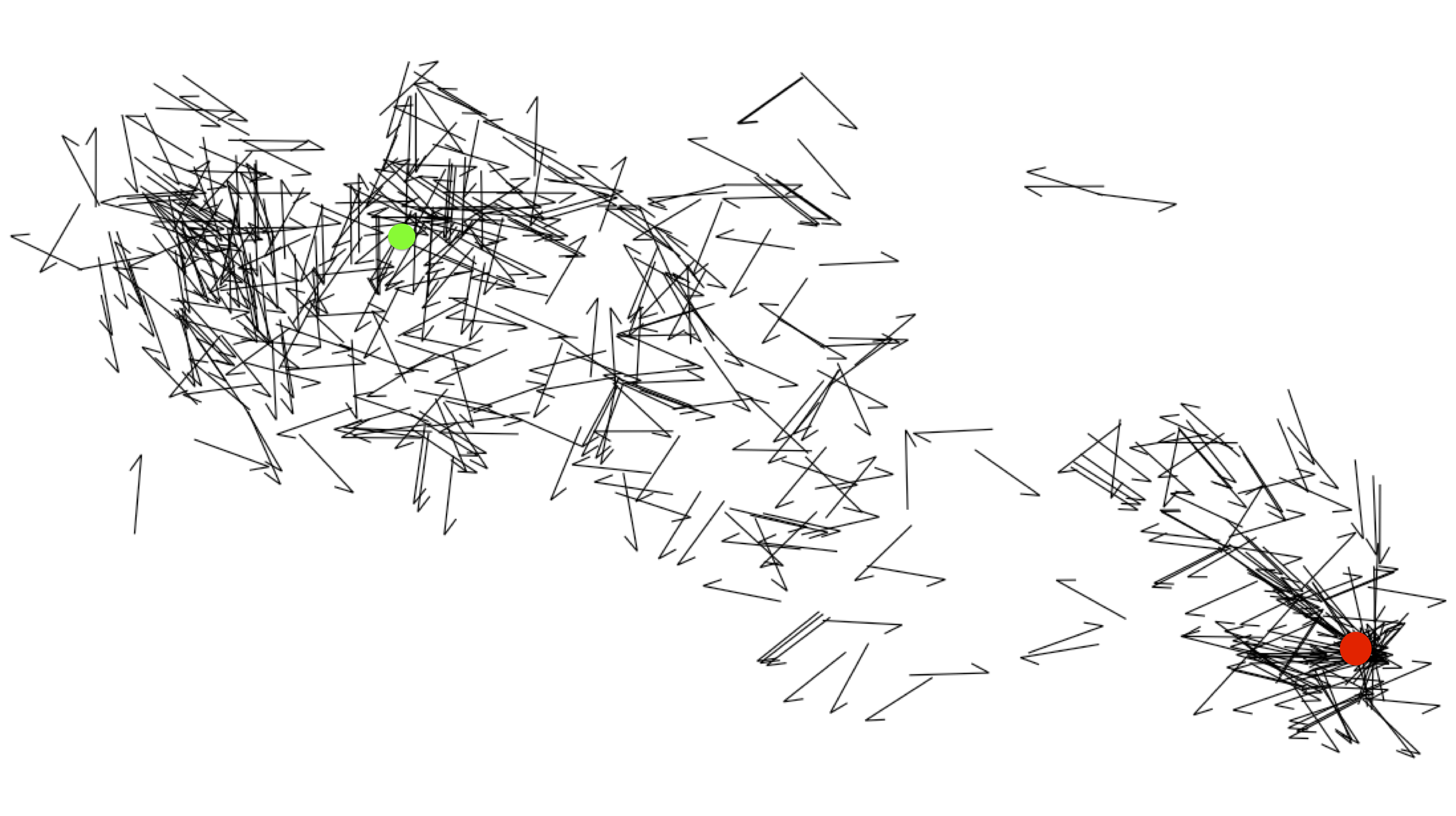
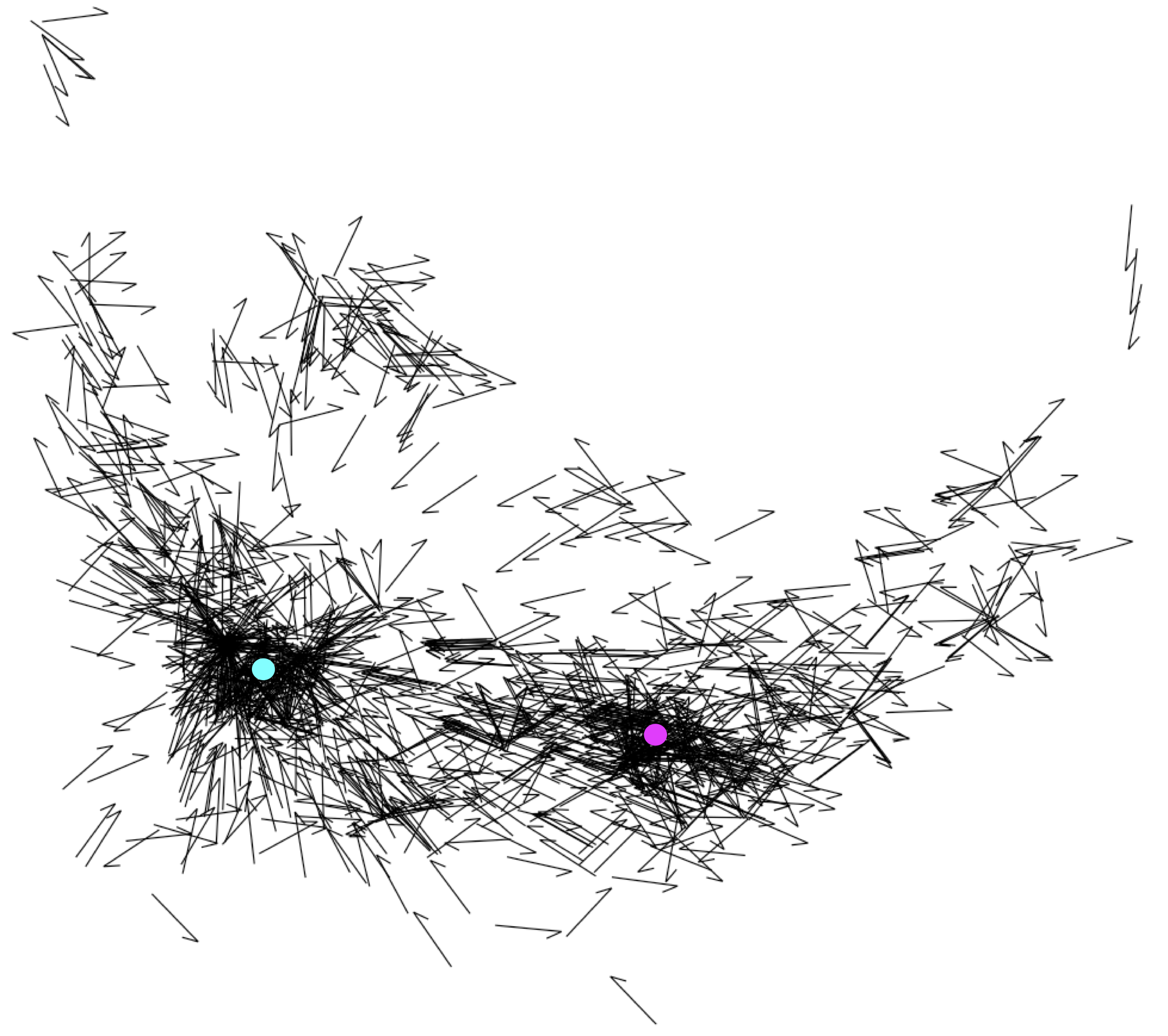
From the remaining locations, crime vectors were constructed to show
which direction the offenders moved when they committed crimes, this
is shown in Figures 3, 4 and
5. Although the data contains other types of crimes, and
even unfounded calls-for-complaints, only the set of events with a
known offender were used.
- 4.5
-
For the models proposed in this paper, we assume that malls are the
major attractors in the region due to the concentration of stores,
restaurants and major transit hubs in their immediate surrounds. We
further assume that, due to extensive work and entertainment
opportunities, many people in the neighbouring municipalities would
define downtown Vancouver as a major activity node in their activity
space. Thus, for North Burnaby we have two malls defined as
attractors. Brentwood Town Centre is located in the north-west area
of the city and Lougheed Town Centre is located in the north-east
part of the city. Finally, downtown Vancouver makes up the third
attractor for this study area. For South Burnaby, Metrotown (located
towards the south-west of the city) and Highgate Mall (located
towards the south-east) are defined as two attractors, in addition
to downtown Vancouver.
- 4.6
-
For Coquitlam we defined Coquitlam Town Centre, the central shopping
mall, as an attractor. We also defined Lougheed Town Centre as an
attractor for this model because it is located just outside the city
limits of Coquitlam. Although Lougheed Town Centre is located in
Burnaby, it is immediately on the border of the City of Coquitlam,
and for all intents and purposes that area cannot be divided (it is
in fact called Burquitlam). For visualization purposes, downtown
Vancouver will not be shown on the images as it would skew the
images too greatly.
- 4.7
-
For visualization purposes, we colour-coded all of the attractors on
the images that display the results for each of the models. The
summary of colours used to identify each attractor is shown in Table
1.
Table 1: The colours and corresponding names of attractors Name of Attractor Colour Downtown Blue Lougheed Town Centre Red Brentwood Town Centre Green Coquitlam Town Centre Yellow Metrotown Cyan Highgate Mall Magenta North Coquitlam Black
Model 1: Home Location and Distance
- 5.1
-
The goal of this paper was to model Crime Locations and the likely
Attractor that influenced the spatial location where the crime
occurred, with respect to the offender's home. The vector connecting
the home and crime locations we refer to as the Crime Vector. There
are several types of locations in any given area which act as
attractors to offenders (e.g., shopping malls). We would like to see
the behaviour of Crime Vectors around these locations.
- 5.2
-
In line with research in environmental criminology, our initial
model consists of just location and distance, and we incrementally
improve our model to include all the aspects which we are interested
in. Instead of analyzing the relationship between Home Location and
distance, like in van Koppen and de Keijser (2006), we are interested in what
attracted the offender to offend at that specific location
based on the distance between the Crime Location and Attractor. By
considering components of the offenders' journeys to crime, we model
the attraction of regional shopping centres in two urban
municipalities in British Columbia: Burnaby and Coquitlam.
- 5.3
-
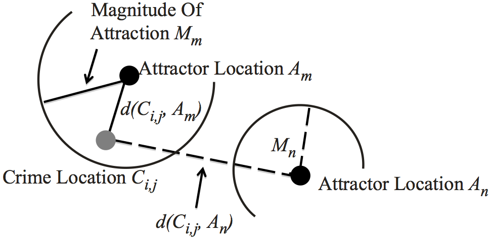
Let us first define the components of the model. There are two sets
of locations which are important with respect to the offenders'
activities. The first is the set of all Crime Locations Ci,j
,
denoting offender i
's crime j
. There are specific locations,
such as shopping malls, that attract offenders to commit crimes.
These are known as Criminal Attractors, or simply Attractors, where
Attractor n
is denoted as An
. In reality these locations are
polygon shapes, but for now we consider them as points, where the
point is at the center of the locations. To determine which is the
primary Attractor, we calculate the distance
d (Ci,j, An)
from
Crime Location Ci,j
to Attractor An
. Each Attractor n
has a
Magnitude Of Attraction, denoted Mn
, which encompasses the area
that An
attracts; the larger the value of Mn
, the stronger the
pull to An
. For the first model, this magnitude of attraction is
fixed. The distance
d (Ci,j, An)
, combined with the Magnitude of
Attraction Mn
for Attractor An
, determines which Attractor
offender i
was moving towards when they committed crime j
. This
is shown in Figure 6.
- 5.4
-
First, in order to mimic the techniques provided by most criminal
researchers studying the Journey to Crime, we define the rules
by which our model will behave. We then construct the model and
apply it to real data. Finally we comment on how well the result
describes the real world environment.
Rules of the Model
- 5.5
-
Given a Crime Location Ci,j
we try to find the Attractor this
offender was attracted to. We use distances between Crime Locations
and Attractors to determine the Magnitude Of Attraction and to
define some rules for finding the Attractor for each crime.
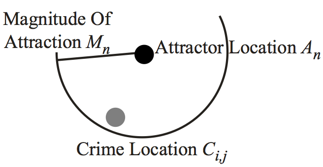
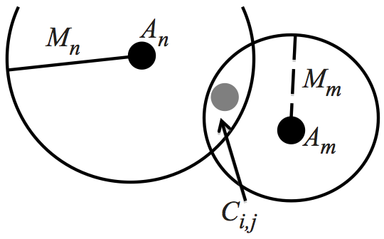
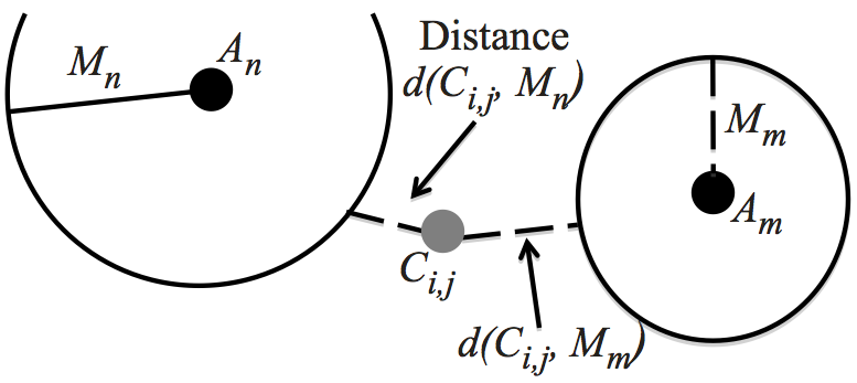
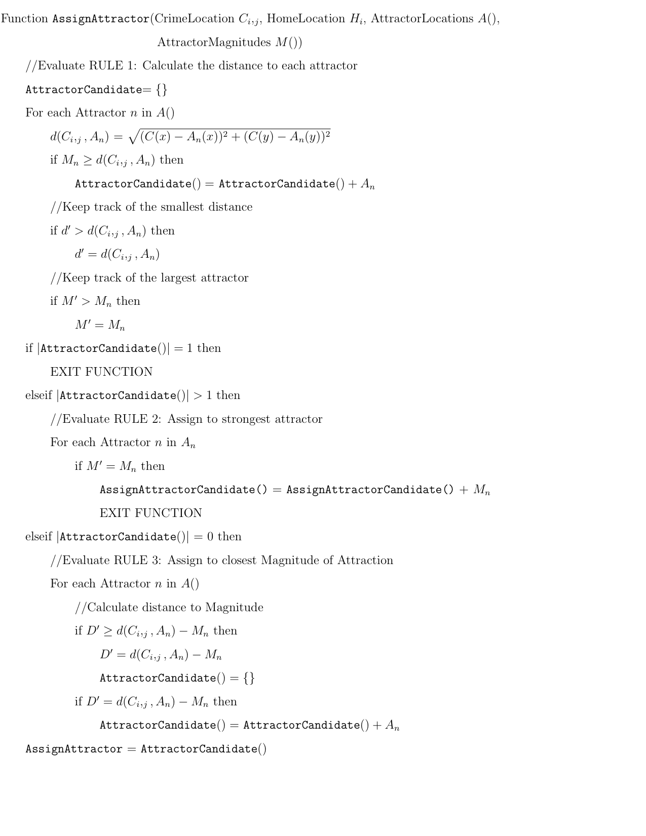
- Rule 1: If Ci,j is inside the Magnitude Of Attraction Mn for a single Attractor An , i.e., Mn > d (Ci,j, An) , then the offender is attracted to this Attractor (Figure 7a).
- Rule 2: If Ci,j is inside the intersection area of the Magnitudes Of Attraction for several Attractors in A , i.e., Mn > d (Ci,j, An) for multiple n , then the offender is attracted to the Attractor with the greatest Magnitude Of Attraction Mn (Figure 7b).
- Rule 3: If Ci,j is outside all the Magnitudes Of Attractions, i.e., Mn < d (Ci,j, An) for all An∈A , then the offender is attracted to the Attractor whose Magnitude of Attraction is closest to the Crime Location, i.e. An for which d (Ci,j, Mn) is minimal. (Figure 7c).
- 5.6
-
The model presented above uses only the distance to each attractor
to determine which location is the likely Attractor for the
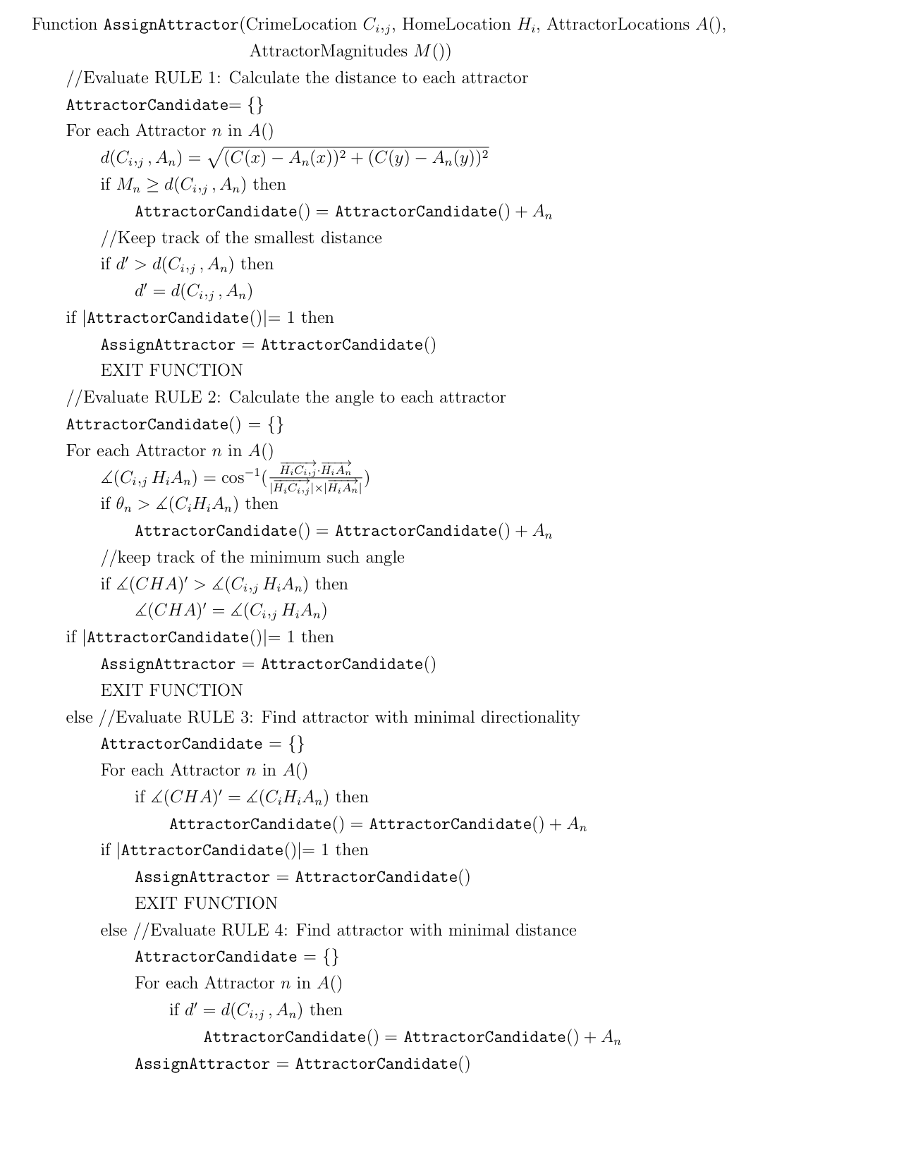
offender. The pseudo-code to calculate this is presented in Figure 8.
Note that ' denotes optimality.
Results
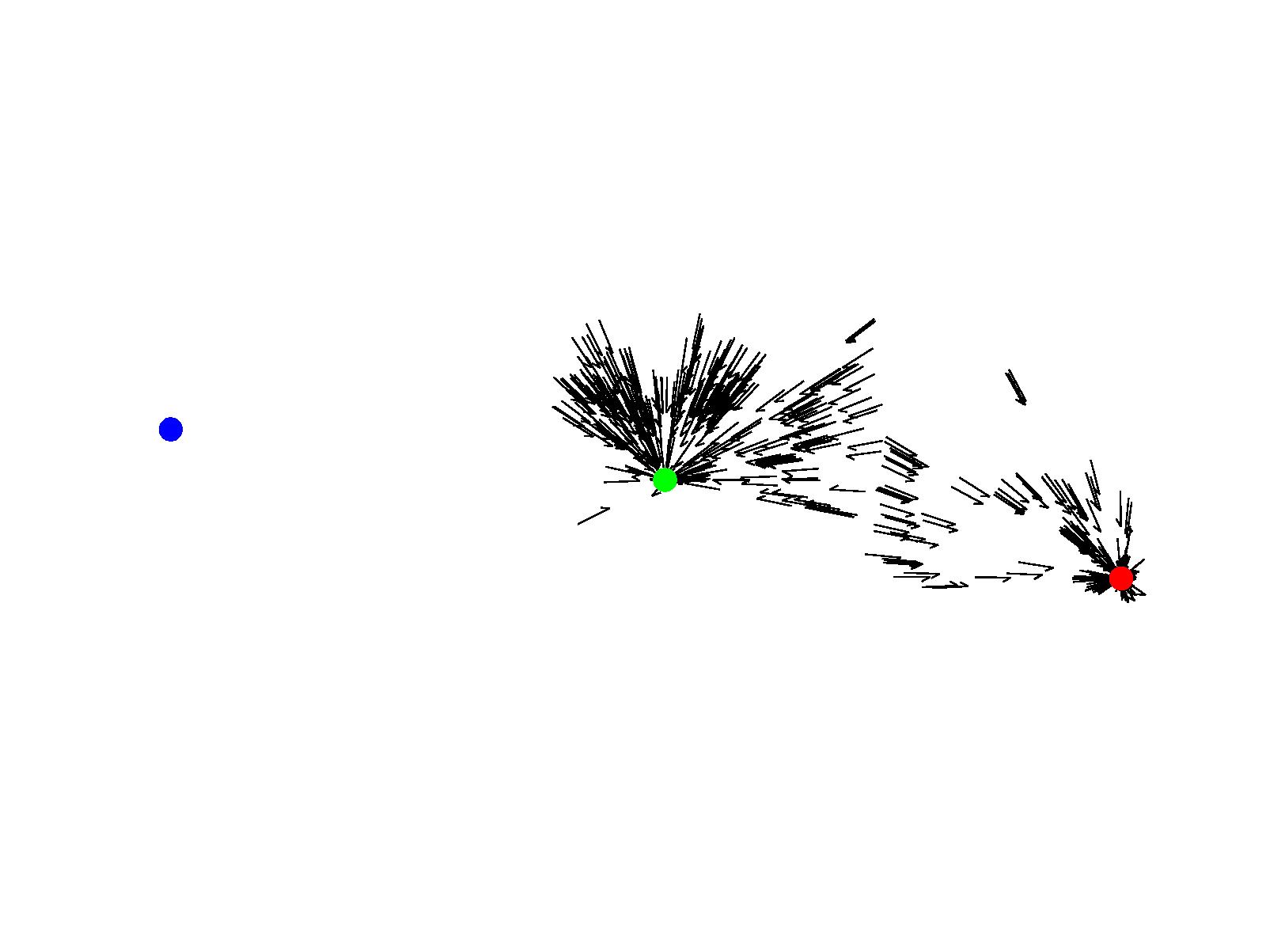
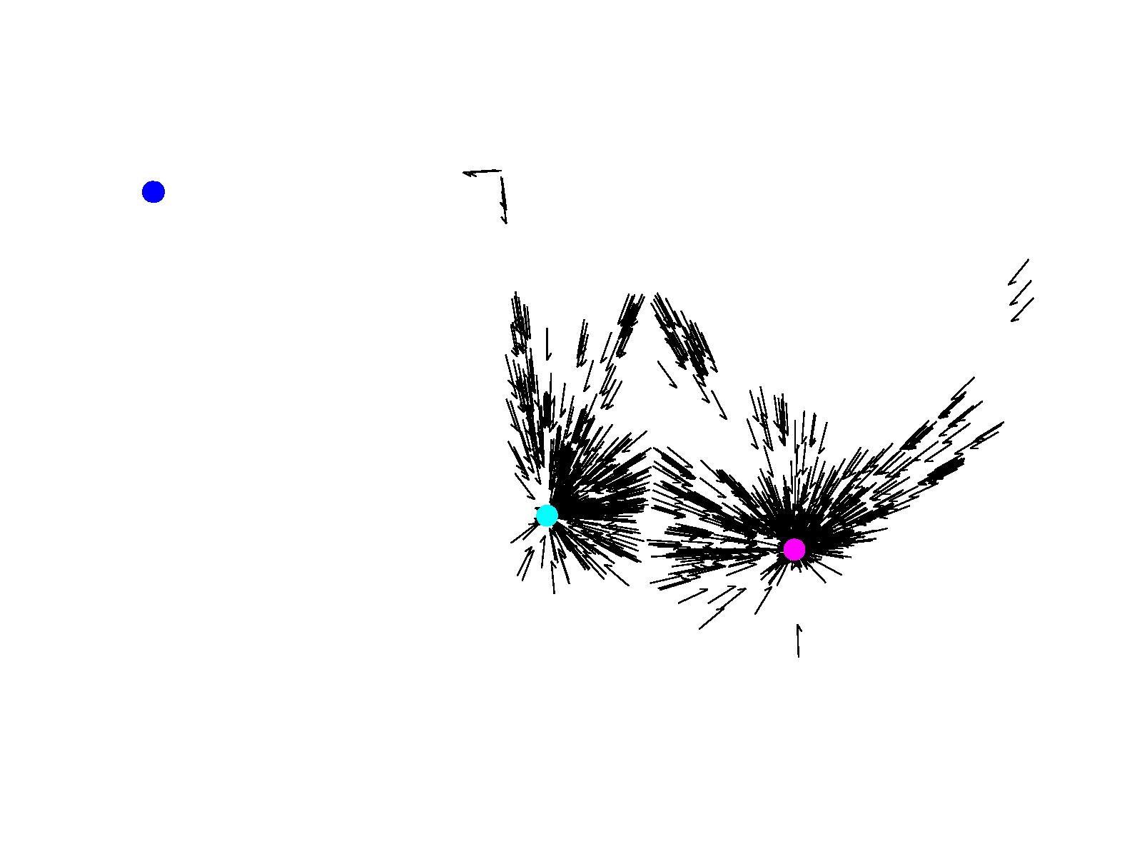
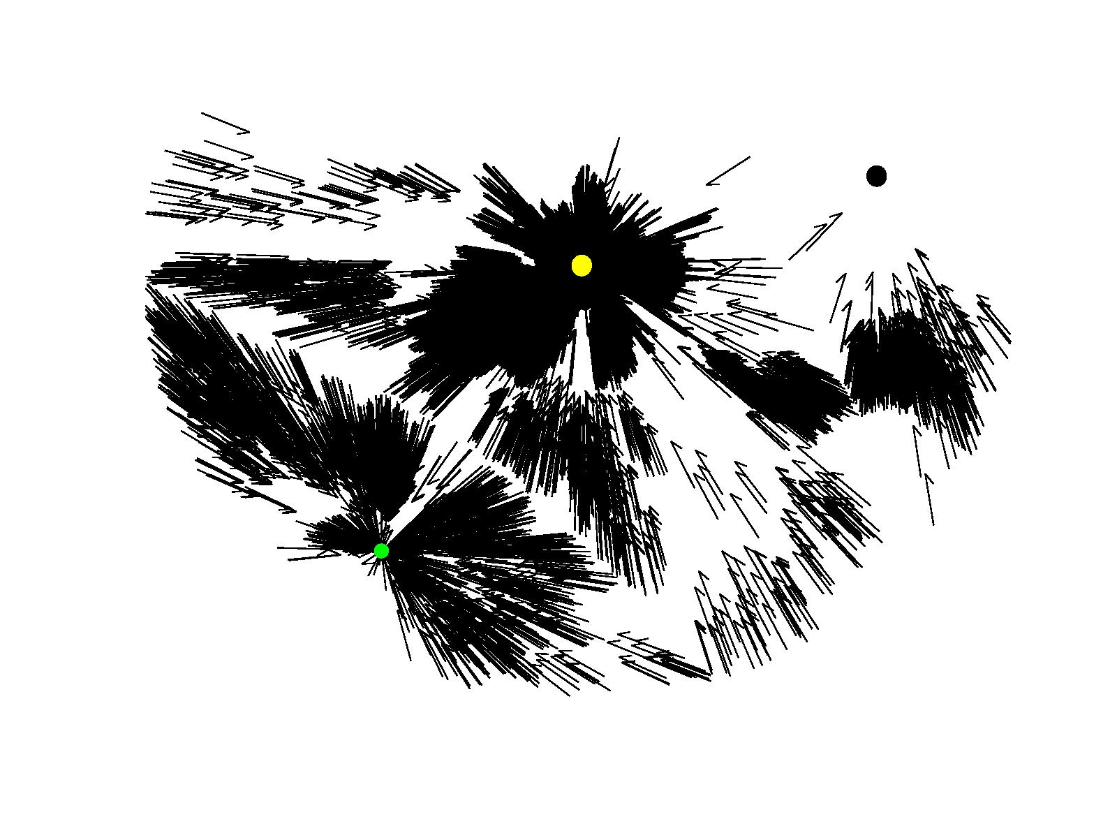
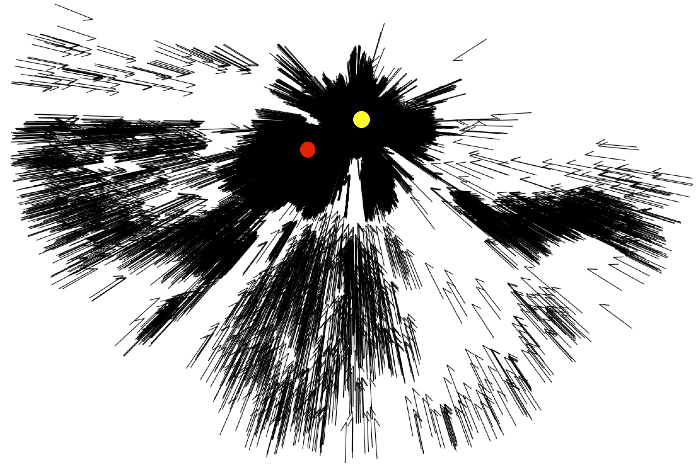
- 5.7
-
Figures 9 to
11 shows the results of
Model 1 applied to our 3 datasets with Mn
fixed to 100. The
locations of the attractors can clearly be identified by the focal
points at which most of the vectors are directed toward. Assigning
the Attractors in this fashion simply results in each Crime Vector
being associated to the closest Attractor. Although possible in real
life, it is probably a bit too naive. The critical component missing
is the inclusion of directionality.
Model 2: The Full Journey to Crime
- 6.1
-
This model includes all of the components of the Journey to Crime by
incorporating directionality into the previous model. In order to do
this, we need to add the Home Location of all offenders, which we
denote with H
, where offender i
resides at Hi
. From Hi
,
two vectors are of importance. First, the Crime Vector, denoted as
 is the vector directed from Hi
towards Ci,j
and denotes the direction from an offender's Home
to the place they committed the crime. Second, the Attractor Vector
is the vector directed from Hi
towards Ci,j
and denotes the direction from an offender's Home
to the place they committed the crime. Second, the Attractor Vector
 is the vector directed from Hi
towards
An
and denotes the direction an Attractor is with respect to the
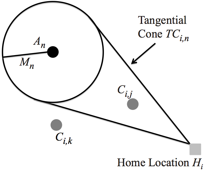
Home of the offender. Third, the Tangential Cone is the cone
projected from H
to the circumference of the Attractor's Magnitude
Of Attraction. Thus, the size of the Tangential Cone from Hi
to
An
is given by
θi,n = sin-1
is the vector directed from Hi
towards
An
and denotes the direction an Attractor is with respect to the
Home of the offender. Third, the Tangential Cone is the cone
projected from H
to the circumference of the Attractor's Magnitude
Of Attraction. Thus, the size of the Tangential Cone from Hi
to
An
is given by
θi,n = sin-1 and is used to denote the relative directional proximity of Hi
to
An
. The larger the Tangential Cone, the closer the directional
proximity is Hi
with respect to An
, given a constant Mn
.
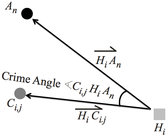
The final component is the Crime Angle
and is used to denote the relative directional proximity of Hi
to
An
. The larger the Tangential Cone, the closer the directional
proximity is Hi
with respect to An
, given a constant Mn
.
The final component is the Crime Angle
 (Ci,jHiAn)
, which is the angle between
and
and is given by
cos-1(
(Ci,jHiAn)
, which is the angle between
and
and is given by
cos-1( ) = tan-1
 - tan-1
 .
.
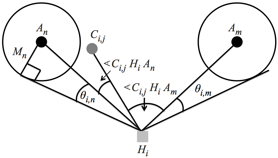
These are illustrated in Figure 12. - 6.2
-
We develop an algorithm to model this. This algorithm gives priority
to the direction along which the crime occurred rather than the
distance between Crime Location and Criminal Attractor.
Rules of the Model
- 6.3
-
Rules are needed to determine which crimes are attracted to which
Attractors. Thus, we define rules to relate the distances between
the Crime Location and Attractor to the Magnitude Of Attraction. We
would say an offender is attracted towards a given criminal
Attractor if the corresponding crime was committed within close
directionality (as opposed to proximity) to the Attractor. That is,
if
(Ci,jHiAn)≤β
, where β
is a
user specified parameter. As an example, all the crime vectors for
the City of Coquitlam are shown in Figure 13a,
while the subset of crime vectors where
(Ci,jHiAn)≤5
are shown in Figure 13b.
Figure 13: Crime vectors of Coquitlam and the criminal attractor 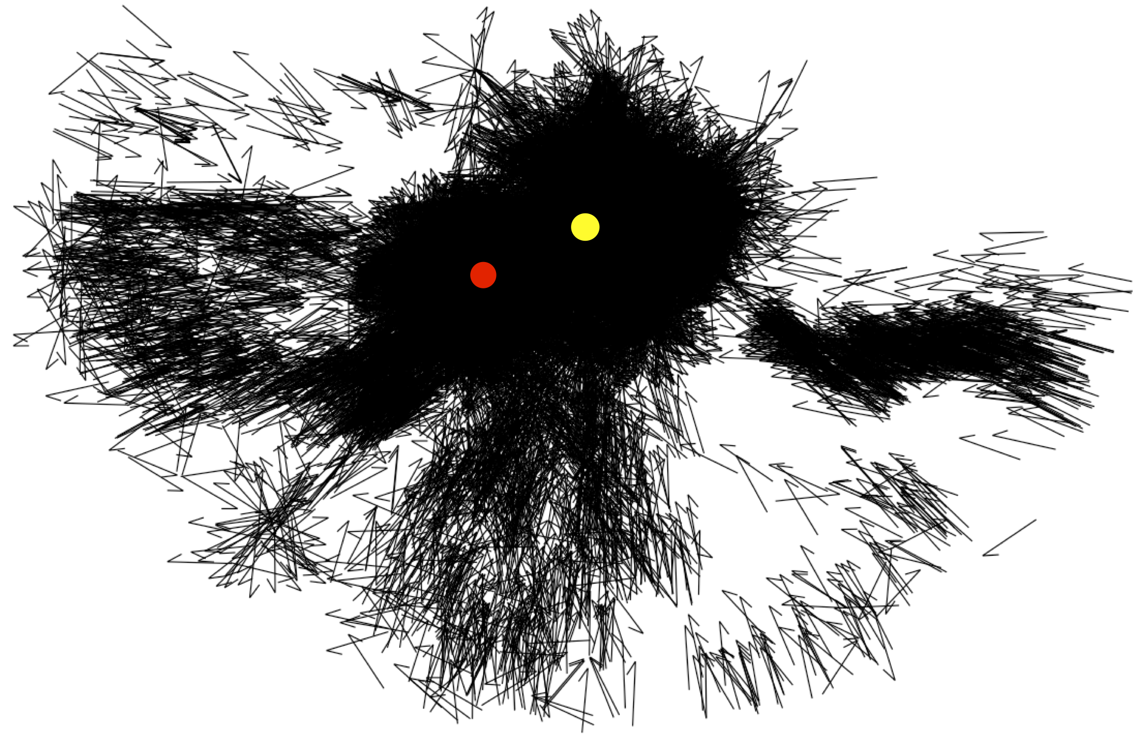
a) Coquitlam crime vectors b) Coquitlam City Center as criminal attractor - 6.4
-
We give the following rules to find the criminal attractor
corresponding to a crime vector. It is easy to understand these
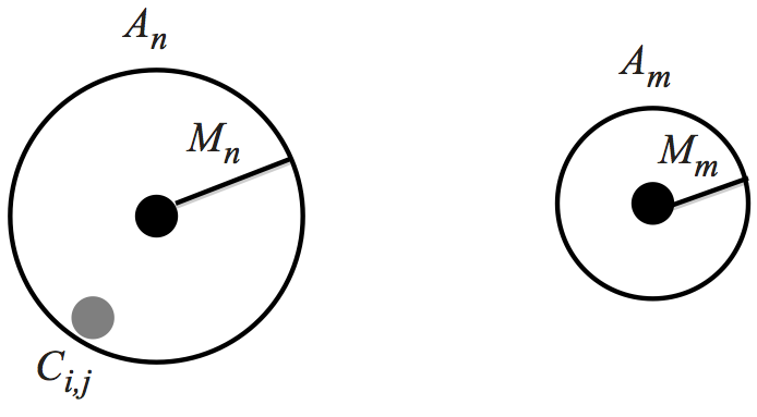
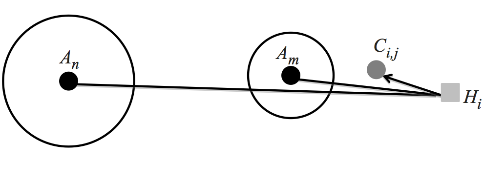
rules visually so we provide Figure 14.
- Rule 1: If the Crime Location is inside the Magnitude of Attraction for a single Attractor, i.e., Mn > d (Ci,j, An) for a single An , then the offender is attracted to this Attractor (Figure 14a).
- Rule 2: If the Crime Vector is outside the Magnitude of Attractions for all A
, then the Crime Vector is
attracted to the attractor with smallest
|(Ci,jHiAn) - θi,n|
, say An
.
For example in
Figure 14b the Crime Vector is closer to the
Tangential
Cone of Attractor An
as
(Ci,jHiAn) < (Ci,jHiAm)
.
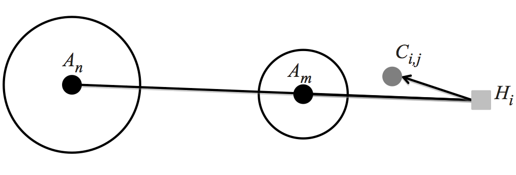
- Rule 3: If the Crime Vector is inside the Tangential Cones of multiple
Attractors in A
then we look strictly at the Crime Angle and
assign the Crime Vector to the Attractor with minimal
(Ci,jHiAn)
. For example, in
Figure 14c the Crime Vector
is inside the Tangential Cones of both Attractors but we observe
that
(Ci,jHiAm) < (Ci,jHiAn)
, hence the Crime Vector is assigned to Am
.
- Rule 4: If the Crime Vector is inside the Tangential Cones of multiple Attractors in A and multiple Attractors have the same minimum Crime Angle, then we look at the distance to the attractor and pick the closest Attractor. For example, in Figure 14d the Crime Vector is inside both Tangential Cones and the Crime Angles are same but the Crime Location is closer to the perimeter of Am hence the Crime Vector is attracted to Am .
- 6.5
-
Although Rules 2 and 3 are similar in meaning, there is a key
difference between them. It is possible that a Crime Location is
close to a weak Attractor, say Am
, but is not in the Tangential
Cone of Am
in which case it would be ignored.
- 6.6
-
The pseudo-code for this algorithm is presented in
Figure 15. Note that ' denotes optimality.
Results
- 6.7
-
In order to maintain clarity in the images, visualizations were
changed from using arrows to using squares and diamonds. We can see
that Model 2 provides some expected results. In North Burnaby there
is a small cluster of crimes formed around the mall towards the east
edge of the city (Figure 16a).
Similarly, the mall towards the west of the city (represented by a
green point) has a cluster of crimes that are attracted to that
Attractor (Figure 16b). Based on the
rules defined for the model, not all crimes are attracted to that
mall. Some (those shown as diamonds) are actually attracted to the
Attractor (downtown Vancouver,
Figure 16c) located far to the west.
- 6.8
-
In South Burnaby we see a somewhat equal distribution of crimes
attracted to each of the attractors. This is expected in this model
because the two malls are assumed to have the same initial level of
attractiveness (Figure 17a-b). They are
also separated by about 5 minutes of travel-time so people can
travel to either one quite easily. Some but not a lot of the
offenders are attracted towards downtown Vancouver
(Figure 17c).
- 6.9
-
Finally, Coquitlam is dominated by Coquitlam Town Centre, and our
model shows the majority of the offenders (shown by diamonds in
Figure 18b) being attracted to it. The
other crimes are relatively evenly spread out to the other two
attractors (Figure 18a and b).
- 6.10
-
What this Model does not deal with is the different strength of
attractiveness, and treats each location identically, hence Mn
was again fixed to 100. However, if a lot of criminals commit crimes
on the way to A1
, but a trivial amount towards A2
, this should
be reflected in the size of attractiveness and A1
should be much
larger than A2
. This is what we call the Magnitude of the Attractor, and is dealt with in Model 3.
Figure 16: Results of North Burnaby using Model 2 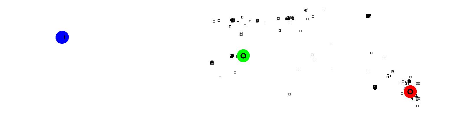
(a) Attractors for Lougheed Town Centre (red) 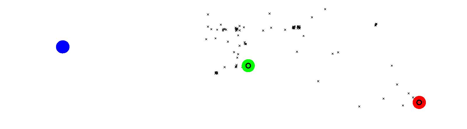
(b) Attractors for Brentwood Town Centre (green) 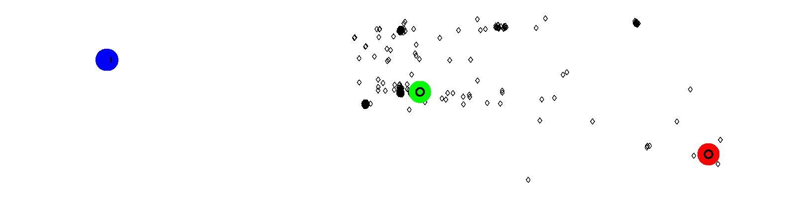
(c) Attractors for Downtown Vancouver (blue) Figure 17: Results of South Burnaby using Model 2 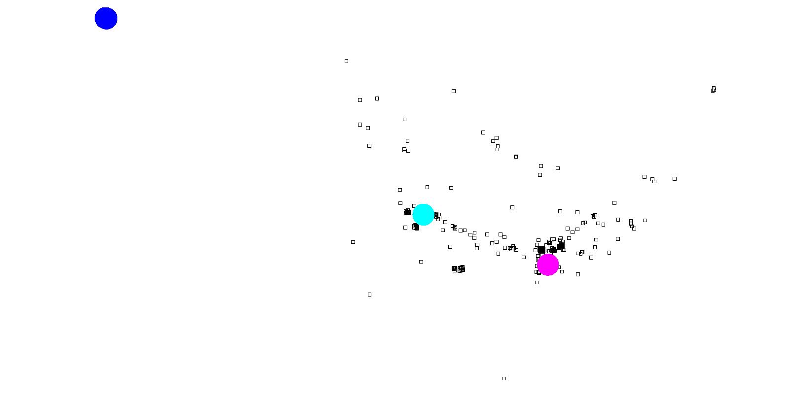
(a) Attractors for Highgate Mall (magenta) 
(b) Attractors for Metrotown (cyan) 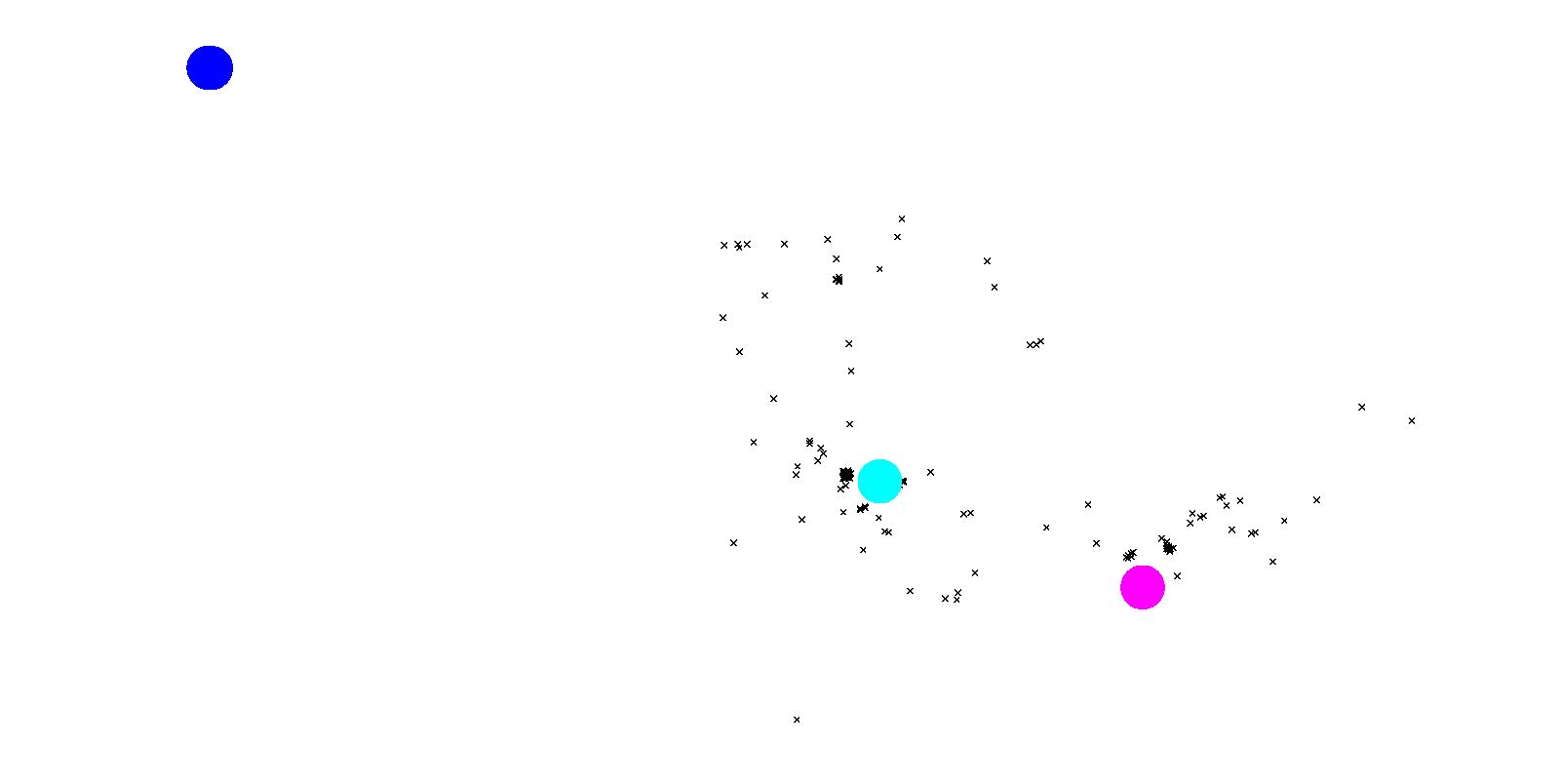
(c) Attractors for Downtown Vancouver (blue) Figure 18: Results of Coquitlam using Model 2 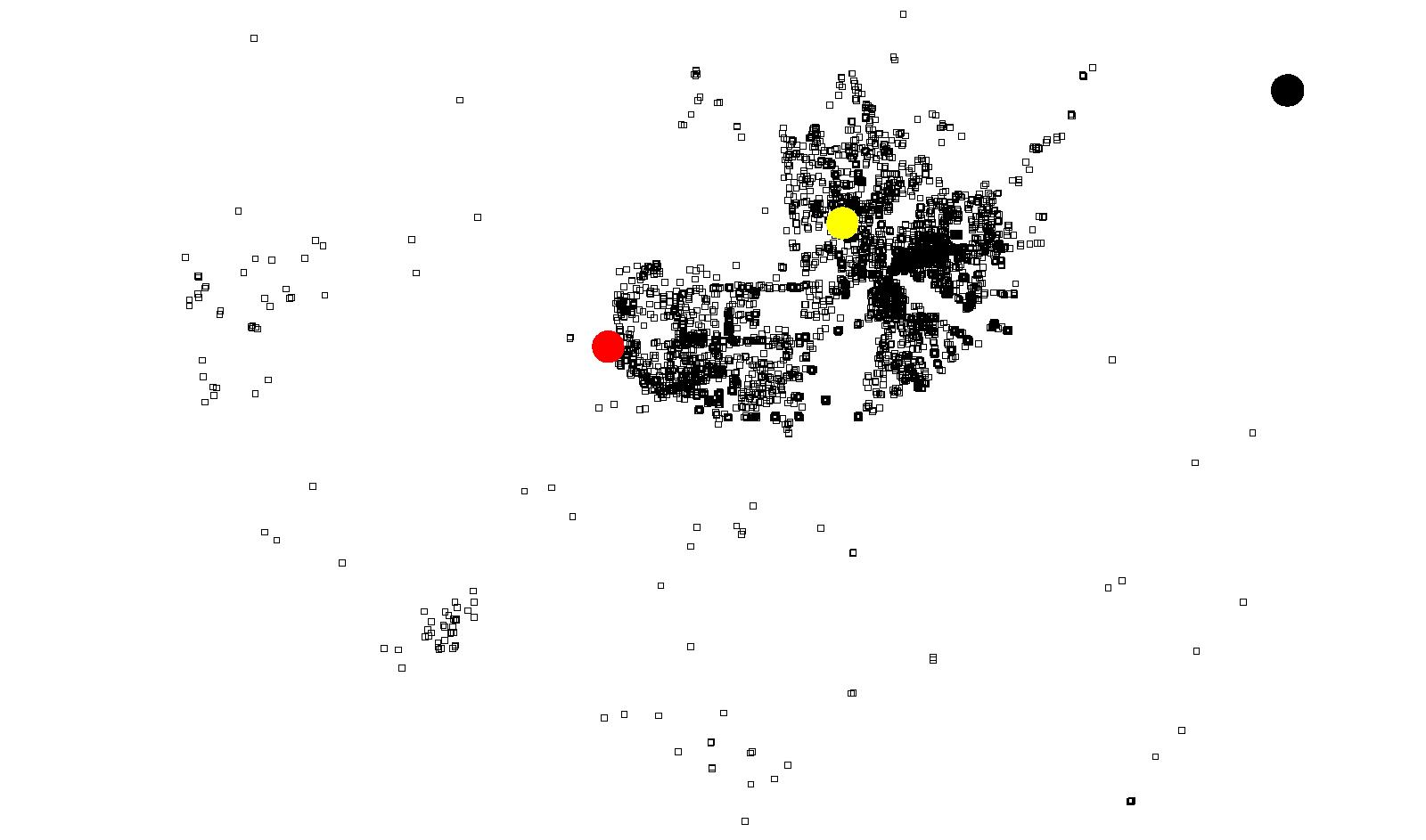
(a) Attractors for Coquitlam Town Centre (yellow) 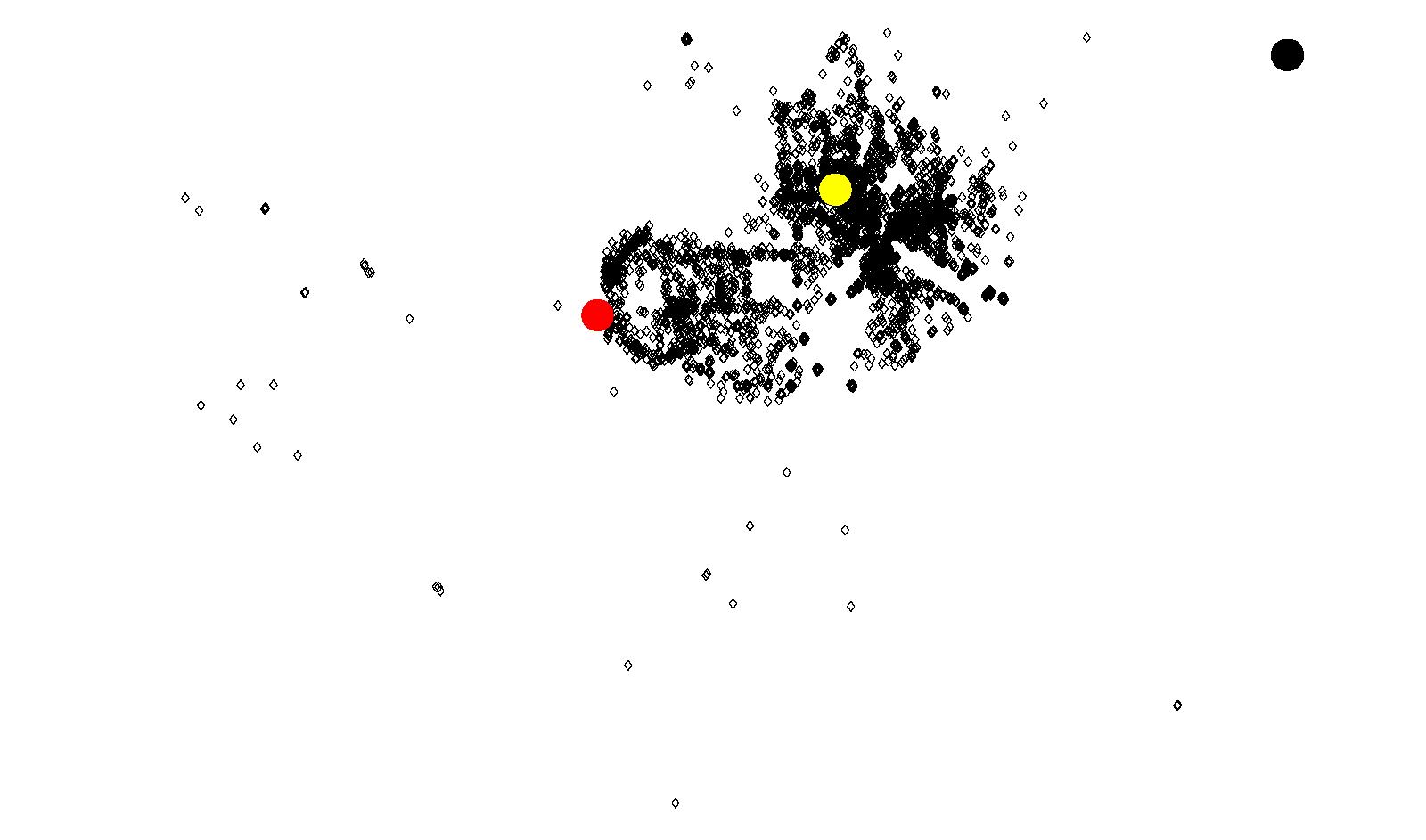
(b) Attractors for North Coquitlam (black) 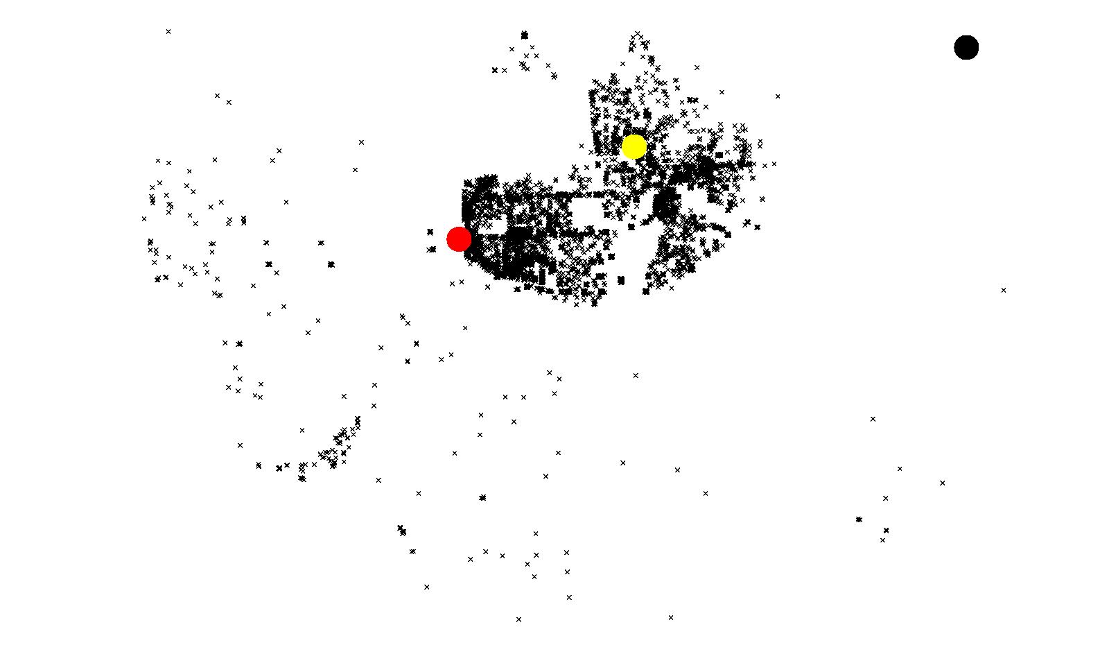
(c) Attractors for Lougheed Town Center (red)
Model 3: Finding the Magnitude of Attractors
- 7.1
-
Until now we assumed that the level of attraction among Attractors
is the same. In Model 3, the initial level of attraction remains the
same among the Attractors but is updated during each iteration of
the algorithm. The algorithm takes these magnitudes as the initial
input values and updates them during each iteration in proportion to
the number of crimes attracted to each Attractor during that
iteration. It terminates if there are no changes from time t
to
t + 1
.
- 7.2
-
Suppose the Magnitude of Attraction at time t
for Attractor An
is Mn(t)
, and the number of criminals attracted to it is
qn(t)
. For example, the number of criminals attracted to
Attractor An
at time t = 0
, the initial state, is qn(0)
.
Knowing that at the beginning of t = 0
the Magnitude of the
Attractor was Mn(0)
, and during that iteration qn(0)
criminals
were attracted to it, we can calculate Mn(1)
as
Mn(1) - Mn(0)∝qn(0).
- 7.3
-
In general, if Mn(t)
and Mn(t + 1)
are the levels of attraction
at t
and t + 1
respectively, and qn(t)
is the number of crimes
attracted to An
at time t
then
Mn(t + 1) - Mn(t)∝qn(t)
or,Mn(t + 1) - Mn(t) = c×qn(t)
HenceMn(t + 1) = Mn(t) + c×qn(t)
where c is some proportionality constant. - 7.4
-
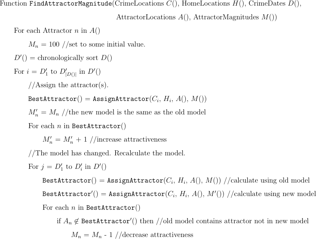
We note the iterative nature of the formula so once we know qn()
for all t
, set some value for the proportionality constant c
and
initial level of attraction we can find the level of attraction for
each Attractor. The pseudo-code for this algorithm is shown in
Figure 19. '
denotes optimality.
- 7.5
-
We simulated the algorithm using real crime locations for North
Burnaby, South Burnaby and Coquitlam. The algorithm was simulated
for two and three attractors.
Model 3 with two Attractors
- 7.6
-
We considered the two largest shopping malls of North Burnaby
(Lougheed Town Centre and Brentwood Town Centre) for the simulation.
Figure 20 shows Lougheed Town Centre and
Brentwood Town Centre as the two attractors, with two concentric
circles denoting their location. The radii of smaller circles
represents the initial level of attraction which we defined to be
100. The larger circles are the output of the algorithm, radii of
which represent the desired level of attraction for each attractor.
We have shown the crime locations with symbols. The squares are the
crime locations which are attracted to Lougheed Town Centre while
the diamonds are the crime locations which are attracted to
Brentwood Town Centre.
Figure 20: North Burnaby property crimes with two attractors 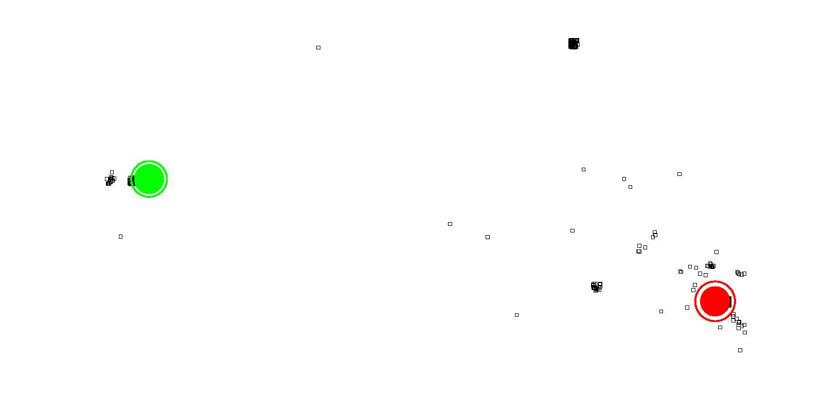
(a) Attractors for Lougheed Town Centre (red) 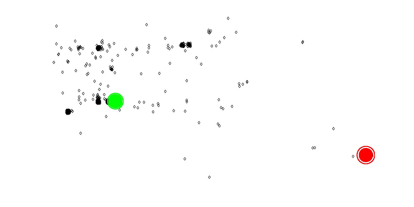
(b) Attractors for Brentwood Town Centre (green) - 7.7
-
The number of crimes attracted to, or the increase in levels of
attraction for each attractor from initial level of attraction
(100), can be a measure of strength/weakness of any attractor.
Table 2 shows the number of crimes
attracted to each attractor and the increase in levels of attraction
for each attractor from the initial level of attraction (100). For
each additional crime that was attracted to an attractor, we
increment the corresponding magnitude of attraction by 1, i.e. our
proportionality constant was set to 1. Although
Figure 20 seems to show otherwise, the actual
numbers indicate that the crimes and increase in levels of
attraction are very similar for both of the attractors. From this,
we can conclude that both are equally strong criminal attractors.
The results are consistent with knowledge of the area, since both
malls are relatively similar in size and contain similar anchor
stores.
Table 2: Number of crimes and levels of attraction for each attractor City Number of
AttractorsAttractor Number of crimes Increase in Magnitude
of AttractionNorth Burnaby 2 Lougheed Town Centre 924 161 North Burnaby 2 Brentwood Town Centre 779 134 North Burnaby 3 Lougheed Town Centre 963 265 North Burnaby 3 Brentwood Town Centre 646 211 North Burnaby 3 Downtown Vancouver 94 118 South Burnaby 2 Highgate Mall 300 181 South Burnaby 2 Metrotown 2710 856 South Burnaby 3 Highgate Mall 268 174 South Burnaby 3 Metrotown 2644 837 South Burnaby 3 Downtown Vancouver 98 126 Coquitlam 2 Coquitlam Center 19778 5930 Coquitlam 2 Lougheed Town Centre 713 1734 Coquitlam 3 Coquitlam Center 9272 3688 Coquitlam 3 Lougheed Town Centre 6973 2458 Coquitlam 3 North Coquitlam 4246 1528 Model 3 with three Attractors
- 7.8
-
Further, we introduce one more attractor in the model, Downtown
Vancouver. Although we do not include crime data for the City of
Vancouver in the current model, it is a suitable Attractor to
include since offenders do not necessarily commit their offences
within the boundaries of their residential municipality.
Furthermore, the work opportunities, shopping and entertainment
districts of Downtown Vancouver attract people from a variety of
municipalities in Vancouver's lower mainland. In
Figure 21 the level of attraction of
Lougheed Town Centre (red), Brentwood Town Centre (green) and
Downtown Vancouver (blue) can be seen. Similar to the previous
model, we initialized the level of attraction with a value of 100
for each attractor. The squares are the crime locations which are
attracted to Lougheed Town Centre, diamonds correspond to Brentwood
Town Centre and crosses correspond to Downtown Vancouver.
Figure 21: North Burnaby property crimes with three attractors 
(a) Attractors for Lougheed Town Centre 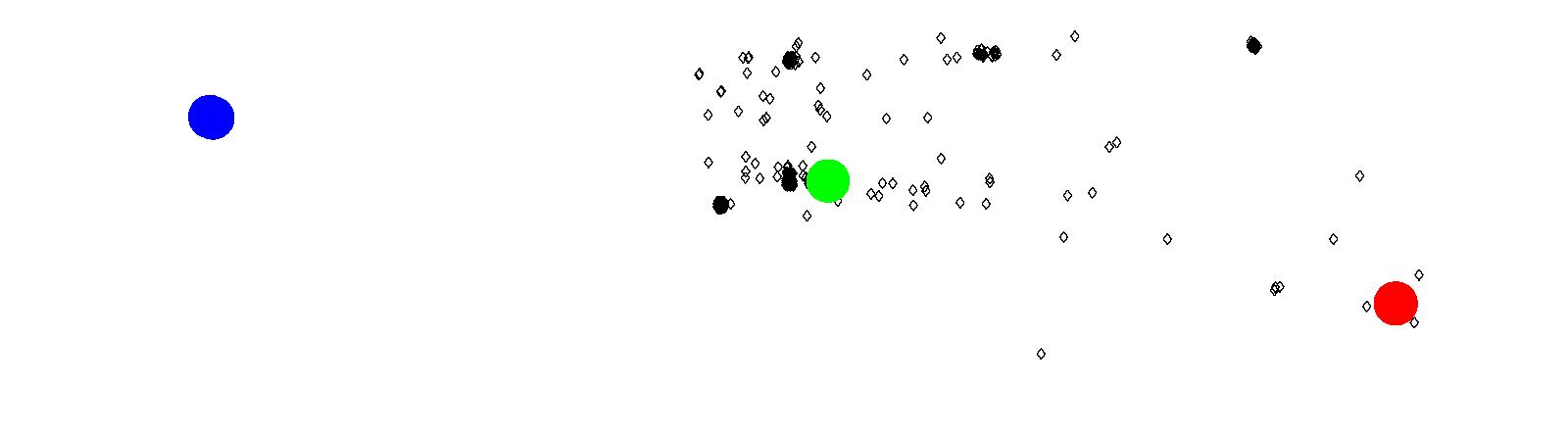
(b) Attractors for Brentwood Town Centre 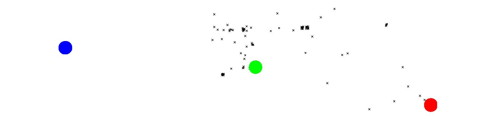
(c) Attractors for Downtown Vancouver Model 3 comparing two and three Attractors
- 7.9
-
Table 2 shows our results for all of the
datasets used for experiments. Figure 21- 23 show the results
pictorially.
- 7.10
-
In North Burnaby, Figure 21, we see that
both Lougheed Town Centre and Brentwood Town Centre are similar in
attractiveness as the amount of crimes attracted to their location
is similar. When downtown Vancouver is introduced as an attractor,
Lougheed Town Centre actually becomes a stronger attractor (39 more
crimes are associated to it), while Brentwood Town Centre becomes
weaker (133 crimes are lost). Downtown Vancouver receives only 94
crimes, which is about a 10th the size of Lougheed Town Centre.
While the two local malls were initially equal, the introduction of
a third attractor shows us that Lougheed Town Centre is more
important of a crime attractor than Brentwood Town Centre is. This
could possibly be explained due to the distant location of Lougheed
Town Center from downtown Vancouver. If offenders living in Burnaby
wish to travel East, they will most likely head towards Lougheed
Town Center, while offenders traveling West will now have a choice
between Brentwood Town Center and Downtown Vancouver.
- 7.11
-
In Figure 22, the two malls, Highgate and
Metrotown, are clearly not of similar scope. Metrotown is the
largest mall in British Columbia, and our results are consistent
with this. Highgate Mall is only a fraction of the size of
Metrotown, and correspondingly its strength as an attractor is also
only a fraction of Metrotown. The introduction of downtown Vancouver
decreases the attractiveness of both malls, as it takes crimes from
both locations equally. Proportionally however, downtown Vancouver
only takes 1% of the crimes from Metrotown, and 11% of the crimes
from Highgate Mall.
- 7.12
-
Coquitlam, Figure 23, is very interesting.
It is very different from the two portions of Burnaby. Coquitlam
Center simply dominates in both instances, when there are two
attractors and when there are three. When there are only two
attractors, compared to Lougheed Town Centre, Coquitlam Center is a
factor of 25 greater of an attractor. When a third attractor is
introduced, the attractiveness of Coquitlam Center is halved, and
this allows Lougheed Town Centre to retain a lot of attractiveness.
What happens in the two-attractor scenario is as follows. The
magnitude of Coquitlam Center is simply so large, that it swallows
up the other attractor. When attractors near Lougheed Town Centre
are evaluated, the magnitude of Coquitlam Center is so large that,
according to our rules, the offender is attracted to it, rather than
Lougheed Town Centre. This is reasonable. If a location is
attractive to criminals, more criminals will likely go there,
increasing its attractiveness further.
Figure 22: Results of South Burnaby using Model 3 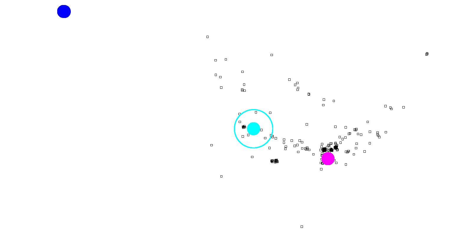
(a) Attractors for Highgate Mall 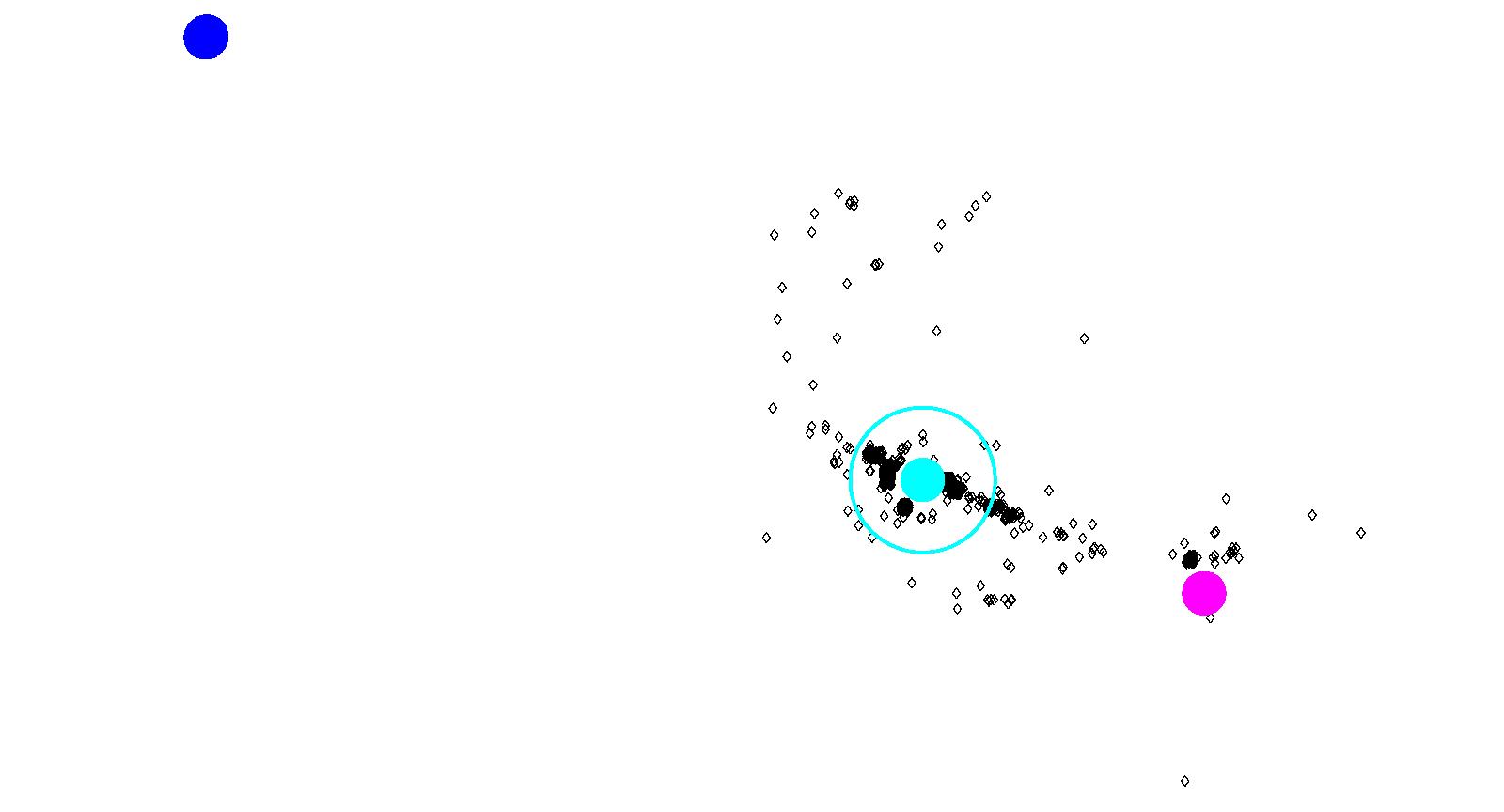
(b) Attractors for Metrotown 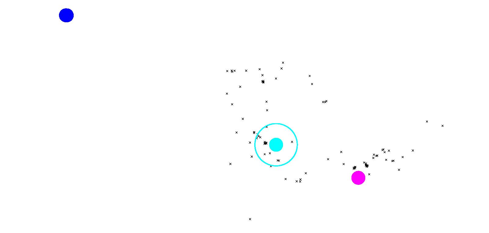
(c) Attractors for Downtown Vancouver Figure 23: Results of Coquitlam using Model 3 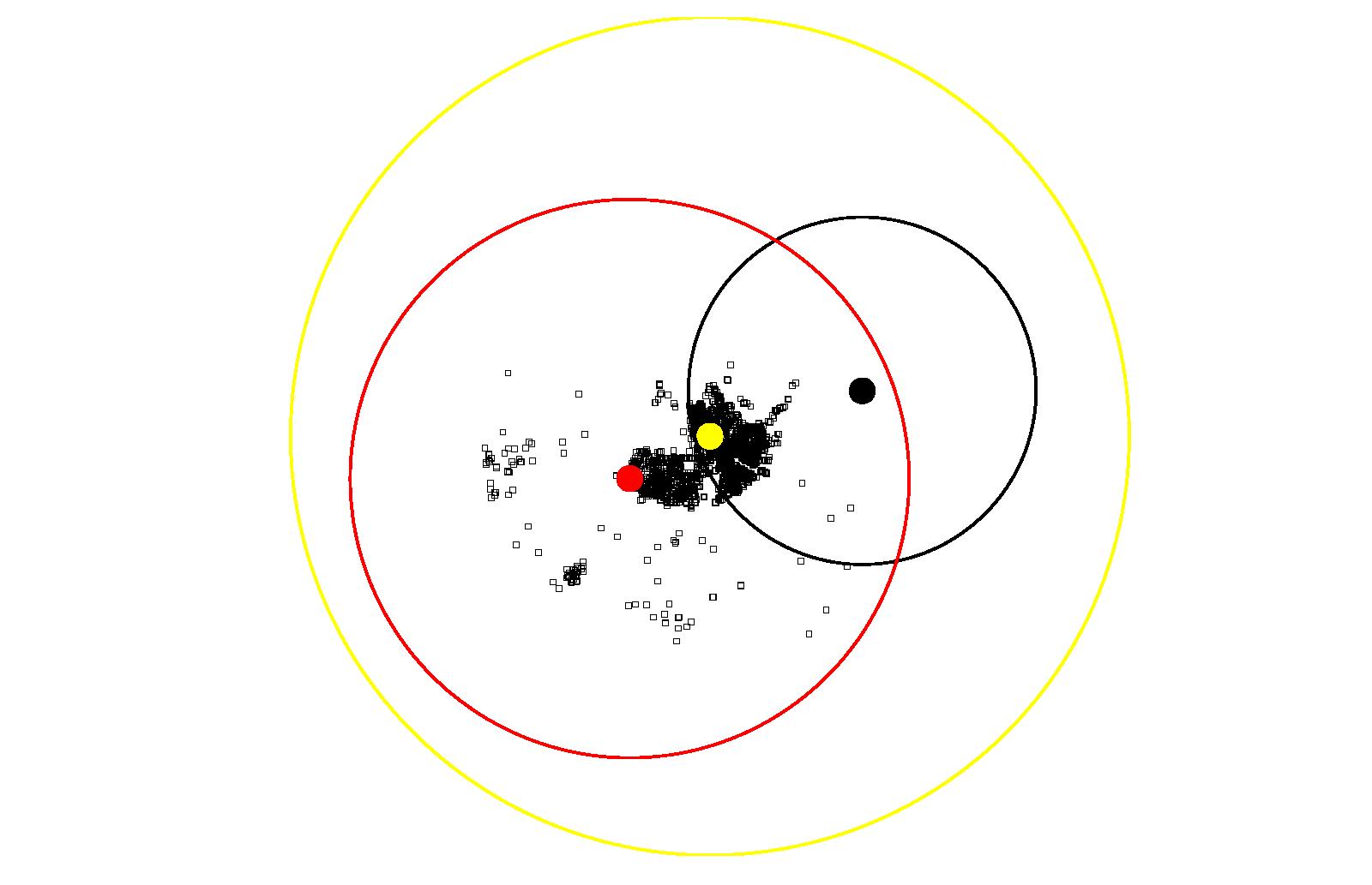
(a) Attractors for Lougheed Town Center 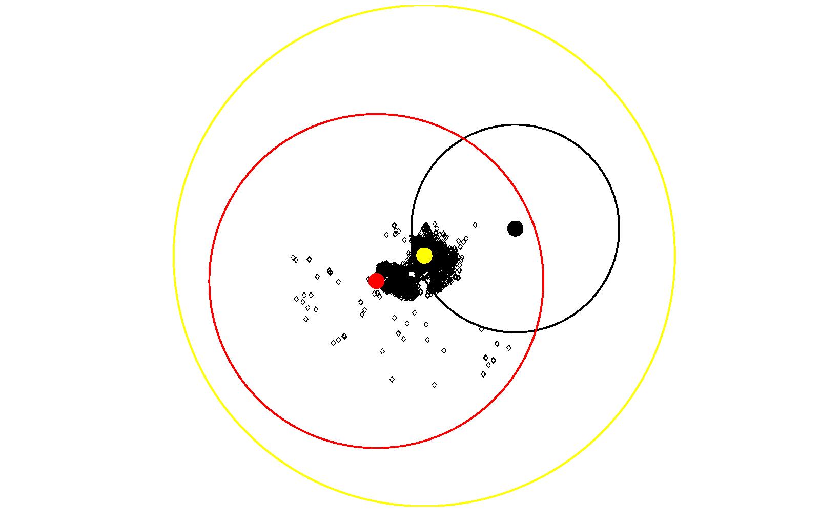
(b) Attractors for North Coquitlam 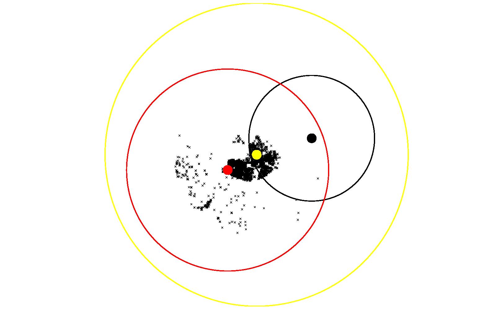
(c) Attractors for Coquitlam Town Center
Discussion
- 8.1
-
These results point to the role of activity nodes, in this case
suburban regional shopping centres, on criminal activity. The
findings suggest an increasing likelihood of crime as a function of
geometric angle and distance from an offender's home location to the
site of the criminal event. This was highlighted, in particular, when
Model 3 was applied to the City of Coquitlam, which resulted in an
overwhelming attractor at Coquitlam Town Centre. This strongly
supports Crime Pattern Theory (Brantingham and Brantingham 1993) which suggests an
underlying pattern to the offense locations should be present. Our
results confirm this.
- 8.2
- The model and its findings may have relevance for real-world issues. Forecasting crime in urban areas is an obvious point of interest for police and city planners, and, given that criminal activity is likely to reduce the success of commercial enterprises in an area, so too for citizens and business owners. The techniques described in this paper may be useful for predicting crime levels in urban areas given the introduction of a new shopping centre, or perhaps other forms of activity nodes. The ability to forecast crime is an invaluable tool that could lead to the prevention of crime. Law-enforcement organizations could use information from criminal activity models such as the one described in this paper to design locally specific crime prevention strategies. This type of proactive policing is gaining favour as decision-makers look for novel crime-reduction and safety promotion strategies. The information provided by this type of modeling research can also be fed into urban land-use policy making. City land-use zoning and policy should consider future consequences of crime when probable criminal attractors are being developed.
Conclusions
- 9.1
-
In this paper, a model was developed to explore the geometric and
geographic determinants of criminal activity in space through an
exploration of crime activity vectors. Offenders' home locations and
the site of their property crimes were extracted from police records
to examine hypotheses of human criminal behaviour. Making use of
Journey to Crime and Activity Space theories used in environmental
criminology, we modeled the relationship between location of
shopping centres, offenders' home location, and the location of
property crimes in two suburban cities, Coquitlam and Burnaby in
British Columbia, Canada. A key advancement of this model to the
environmental criminology literature was the focus on geometric
directionality as a potential determinant of criminal activity
locations.
- 9.2
-
There is growing interest in modeling criminal activity patterns, as
police, policy makers, and government look for new methods to better
understand crime patterns which could ultimately lead to crime
reduction. The model described in this paper represents a starting
point for future research. Plans are being made to extend the
directionality model described herein in order to deal with changes
to the system, such as the addition or removal of an activity node,
or changes to the urban infrastructure. This will be particularly
useful for examining future consequences of urban policy decisions.
Similar to this idea, we would like to see if the model can pick
up seasonal or annual trends, or simply changes in the attractors as
time progresses. In the existing models the Attractors were given to
the model. We are searching for ways of determining the locations of
those Attractors based on the real world crime data. Once locations
are determined, the model presented above can be applied to
determine its strength.
- 9.3
-
The road-network is an important consideration when analyzing
patterns in urban areas. In the future, the theories presented in
this paper will be modified to deal with the complexities introduced
by the road-network. One such complexity is the varying
directionality present as a road winds from one point to another. In
extreme cases, it is possible that the shortest path between a
source and target actually initially leads away from the target.
- 9.4
-
Finally, in order to validate the model in a more complete fashion,
but without waiting for future events to occur, the next task will
be to validate this model using cross-validation where the dataset
available is split into n portions, where n-1 are used
to build the model with the remaining portion used for validation
(repeating n times, each time leaving a different portion for
validation). This way the predicted magnitude of strength can be
considered against each result from the dataset.
Acknowledgements
-
The project was supported in part by the CTEF MoCSSy Program and the ICURS research center at Simon Fraser University. We also are grateful for technical support from The IRMACS Centre also at Simon Fraser University. Finally, we would like to express our gratitude for the helpful feedback from our referees.
Notes
- 3
- This simple summary of the factors that determine the spatial patterning of crimes does not account for more complex target selection behaviour that is found with multiple (co-) offenders (see Brantingham and Brantingham (1981) for a more detailed discussion of the target selection behaviour of criminals).
References
-
A. Alimadad, P. Borwein, P.L. Brantingham, P.J. Brantingham, V. Dabbaghian-Abdoly, R. Ferguson, E. Fowler, A.H. Ghaseminejad, C. Giles, J. Li, N. Pollard, A. Rutherford, A. van der Waall, Using Varieties of Simulation Modeling for Criminal Justice System Analysis, In L. Liu and J. Eck (Eds.), Artificial Crime Analysis Systems: Using Computer Simulations and Geographic Information Systems, Idea Press, Hershey, PA, (2008). [doi:10.4018/978-1-59904-591-7.ch019]
J.D. Alston., The serial rapist's spatial pattern of target selection, Unpublished Thesis, Simon Fraser University, Burnaby, B.C., (1994).
N.M. Argent and D.J. Walmsley, From the Inside Looking out and the Outside Looking in: Whatever Happened to 'Behavioural Geography'? Geographical Research, 47(2) (2009), 192–203. [doi:10.1111/j.1745-5871.2009.00571.x]
W. Bernasco and F. Luykx, Effects of Attractiveness, Opportunity and Accessibility to Burglars on Residential Burglary Rates of Urban Neighborhoods, Criminology, 41 (2003), 981–1001. [doi:10.1111/j.1745-9125.2003.tb01011.x]
BCStats, 2006 Census of Canada: Census Profiles, Retrieved 20 November, 2009, from http://www.bcstats.gov.bc.ca/data/cen06/profiles/detailed/ch_alpha.asp
BCStats, Population Estimates: Municipalities, Regional Districts and Development Regions, Retrieved 20 November, 2009, from http://www.bcstats.gov.bc.ca/DATA/pop/pop/mun/PopulationEstimates_1996-2008.pdf
P.L. Brantingham and P.J. Brantingham, Notes on the geometry of crime, In P.J. Brantingham and P.L. Brantingham (Eds.), Environmental Criminology, Sage Publications, Beverly Hills, CA, (1981).
P.L. Brantingham and P.J. Brantingham, Environment, routine, and situation: Toward a pattern theory of crime, In R.V. Clarke and M. Felson (Eds.), Routine Activity and Rational Choice: Advances in Criminological Theory, (5th Ed.), Transaction Publishers, New Brunswick, NJ, (1993).
P.L. Brantingham and P.J. Brantingham, Criminality of place: Crime generators and crime attractors, European Journal of Criminal Policy and Research, 3 (1995), 5–26. [doi:10.1007/BF02242925]
P.J. Brantingham and G. Tita, Offender mobility and crime pattern formation from first principles, In L. Liu and J. Eck (Eds.), Artificial Crime Analysis Systems: Using Computer Simulations and Geographic Information Systems, Idea Press, Hershey, PA, (2008). [doi:10.4018/978-1-59904-591-7.ch010]
P.J. Brantingham, P.L. Brantingham, and P.S. Wong, How public transit feeds crime: Notes on the Vancouver ''Skytrain'' experience, Security Journal, (2)2, (1991), 91–95.
R.D.F. Bromley and A.L. Nelson, Alcohol-related crime and disorder across urban space and time: Evidence from a British city, Geoforum, 33 (2002), 239–254. [doi:10.1016/S0016-7185(01)00038-0]
L.A. Brown, E.J. Malecki and S.G. Philliber, Awareness space characteristics in a migration context. Environment and Behavior, 9(3) (1977), 335–348. [doi:10.1177/001391657700900303]
E.W. Burgess, Can neighborhood work have a scientific basis?, In Park, R.E., Burgess, E.W., McKenzie, R. (Eds.), The City, University of Chicago Press, Chicago, (1925).
V. Dabbaghian, P. Jackson, K. Wuschke and V. Spicer, A cellular automata model on residential migration in response to neighbourhood social dynamics, Math. Comput. Modelling, 52 (2010), 1752 – 1762. [doi:10.1016/j.mcm.2010.07.002]
C. Gerritsen Caught in the Act: Investigating Crime by Agent-Based Simulation Ph.D. Thesis. VU University Amsterdam, (2010)
R.G. Golledge, J.S. Neil, and B.B. Paul, Behavioral Geography. In International Encyclopedia of the Social & Behavioral Sciences, (2001) (pp. 1105–1111). Oxford: Pergamon. [doi:10.1016/B0-08-043076-7/02491-8]
R.G. Golledge and R.J. Stimson, Spatial Behavior: A Geographic Perspective, New York: Guilford Press, (1997).
E.R. Groff, The Geography of Juvenile Crime Place Trajectories Masters Thesis, University of Maryland, (2005)
J.B. Kinney, P.L. Brantingham, K. Wuschke, M.G. Kirk, and P.J. Brantingham, Crime attractors, generators and detractors: Land use and urban crime opportunities, Built Environment, 34 (2008), 62–74. [doi:10.2148/benv.34.1.62]
J.A. Kopec, Concepts of disability: The activity space model, Social Science and Medicine, 40(5) (1995), 649–656. [doi:10.1016/0277-9536(95)80009-9]
P.J. van Koppen and J.W. de Keijser, Desisting distance decay: On the aggregation of individual crime trips, Criminology 35/3 (2006) pp 505-515 [doi:10.1111/j.1745-9125.1997.tb01227.x]
X. Li, Simulating Urban Dynamics Using Cellualar Automata, In L. Liu and J. Eck (Eds.), Artificial Crime Analysis Systems: Using Computer Simulations and Geographic Information Systems, Idea Press, Hershey, PA, (2008). [doi:10.4018/978-1-59904-591-7.ch007]
K. Lynch,The Image of the City, Cambridge, MA: MIT Press, (1960).
N. Malleson and P. Brantingham Prototype Burglary Simulations for Crime Reduction and Forecasting. Crime Patterns and Analysis (2008) 2(1), 47-66.
M.J. Mason and K. Korpela, Activity spaces and urban adolescent substance use and emotional health, Journal of Adolescence, 32(4) (2009), 925–939. [doi:10.1016/j.adolescence.2008.08.004]
M.H. Matthews, Children represent their environment: Mental maps of Coventry city centre, Geoforum, 11(4) (1980), 385–397. [doi:10.1016/0016-7185(80)90025-1]
R. Mercado and A. Pimez, Determinants of distance traveled with a focus on the elderly: a multilevel analysis in the Hamilton CMA, Canada Journal of Transport Geography, 17(1) (2009) 65–76. [doi:10.1016/j.jtrangeo.2008.04.012]
C. Morency, A. Paez, M.J. Roorda, R. Mercado and S. Farber, Distance traveled in three Canadian cities: Spatial analysis from the perspective of vulnerable population segments, Journal of Transport Geography, (2009), In Press.
R.K. Rai, M. Balmer, M. Rieser, V.S. Vaze, S. Schonfelder and K.W. Axhausen, Capturing human activity spaces - New geometries, Transportation Research Record (2021), (2007), 70–80. [doi:10.3141/2021-09]
J.H. Ratcliffe, Geocoding crime and a first estimate of a minimum acceptable hit rate., International Journal of Geographical Information Science, (2004), 18:61-72. [doi:10.1080/13658810310001596076]
G.F. Rengert and J. Wasilchick, Suburban Burglary: A Time and a Place for Everything, Charles C. Thomas, Springfield, IL, (1985).
G.F. Rengert, The journey to crime, In G. Bruinsma, H. Elffers, and J.D. Keijser (Eds.), Punishment, Places and Perpetrators: Developments in Criminology and Criminal Justice Research, Willan, Cullompton, Devon, (2004).
L.W. Sherman, P.R. Gartin, and M.E. Buerger, Hot spots of predatory crime: Routine activities and the criminology of place, Criminology, 27 (1989), 27–55. [doi:10.1111/j.1745-9125.1989.tb00862.x]
P. Wiles and A. Costello, The road to nowhere: The evidence for traveling criminals, U.K. Research study 207, Home Office, Research, Development and Statistics Directorate, London, (2000).