Abstract

Land acquisition and ownership is an important part of modern agriculture in North America. Given the unique nature of farmland as a good, this paper develops a multi-agent simulation of farmland auction markets in a Canadian context. The model is used to generate data on land transactions between farm agents to determine if a particular auction design or type is better suited to farmland transactions. The simulation uses three different sealed-bid auctions, as well as an English auction. The auctions are compared on the basis of efficiency, stability, and perceived surplus. We find that the form of agent learning about land markets affects both sale price and the variance of sale prices in all of the studied auctions. The second-price-sealed-bid auction generates the most perceived surplus, most equitable share of surplus, and also decreases uncertainty in the common-value element of prices. But on a macroscopic level, it appears that auction choice does not influence market structure or evolution over time.

Keywords:

Multi-Agent Simulation, Auctions, Agriculture

Introduction

1.1

Agriculture as an industry in North America is going through a major period of transition. Technological changes continue to create to significant economies of scale at the farm level, leading to greater competition for farm land. Farming is also affected by increasing price volatility in both input and output markets. Nowhere are these changes affecting production more than in the Prairie provinces, the agricultural heartland of Canada.

1.2

Since land acquisition is so critical to modern agriculture, this paper examines the efficiency of auction markets to sell farmland. Using simulation allows us to incorporate factors such as individual heterogeneity, variable feedback, strategic behaviour, and agent learning into standard static auction models. Several well-known auction types will be compared via multi-agent simulation to assess which is best suited to selling farmland, where each auction type will be evaluated based on pricing efficiency and the generation of surplus. We also incorporate the effects of agent-level decision making on macro level variables in farmland markets, a factor that has not been well considered in agricultural research.

1.3

While there are agricultural models incorporating farmland auctions within the framework of multi-agent simulation (Balmann 1997; Freeman et al. 2009), the comparative efficiency of land auctions was not the focus of these prior efforts. The contribution of this research is to examine the effects of auction choice on market structure and economic efficiency in agricultural land transactions. Farm exits, financial stability, productivity, price levels, transaction surplus, and price variability will be tracked to determine which auction mechanism is best suited for selling farmland. Finally, while some research has modeled "auction-like" land markets that incorporate space and time (Balmann 1997), and others have focused specifically on the design of farmland auctions (Colwell and Yavas 1994), to our knowledge no work has yet analyzed a realistic farmland auction market capturing both space and time.

1.4

This paper is drawn from the unpublished thesis of Arsenault (2007) and is organized as follows. We begin with a broad outline of the conceptual model of farming and land markets applicable to Canadian Prairie agriculture. This leads to a more formal description of the simulation environment and the equations used to govern farm agent behaviour. The latter section includes some rationale about farm agent learning in the context of land auction participation. The auction/bidding models and algorithms used in this simulation are covered next, followed by a brief description of the simulation environment. Subsequently, key findings are highlighted and contextualized within the framework of the efficiency of agricultural land auctions for both buyer and seller. The paper then concludes.

Conceptual Framework

2.1

In today's electronic world, auctions are commonplace and used to sell a variety of goods on very different scales, from household items on E-Bay to regional radio spectrum licenses across the globe (Klemperer 2002). But when Vickrey (1961) first wrote an economic theory of auctions, he did so under the assumption of independent private valuations among the participants of the good being auctioned. Simply put, Vickrey assumed that bidders in an auction value a good independently of other bidders over the same good. Clearly this assumption may not hold for all goods sold in auction markets.

2.2

Farmland is one good that does not readily fit within the independent private values model. Firstly, farmland is a capital asset that can be resold in the future. It is long-lived and generates income over time. It is also fixed in space and thus cannot be transported. For these reasons, time and space matter for farmland markets. It is the combination of these qualities that make farmland very distinct from typical consumption goods (say, like toys or furniture), meaning that an auction design for farmland based on a one-time independent private values assumption may not be appropriate.^[1]

2.3

However, one of the most important features of farmland concerns its affiliated values characteristics. As an example, under an affiliated values assumption, a given individual's personal valuation for a plot of farmland is now both a function of their private valuation and a common valuation, the latter being observed or learned from prior transactions and bidding behaviour. The affiliated values assumption greatly complicates the design of optimal auctions since noisy common value observations cause uncertainty and decrease efficiency (Goeree and Offerman 2002). Due to these unique characteristics, designing an optimal auction mechanism for farmland would necessarily be complex in a computational sense. This is the reason we choose to examine the issue of auction design for farmland via multi-agent simulation.

2.4

The multi-agent simulation model assessing the relative efficiency of farmland auctions is built upon a series of relatively simple relationships or equations governing the behaviour of each farm agent. In addition, every time period agents make calculated decisions based on individual experiences and expectations, and these decisions in turn also affect the decisions of all other agents in future time periods.

2.5

A flowchart (Figure 1) helps outline the major activities undertaken by the agents in the simulation. Farm agents start in what we refer to as a Crop Production Module, where all production, harvesting, and crop sale activities take place. Agents then progress to what we call the Farm Finances Module where they determine if they should remain in the land market or exit.

2.6

In any given time period, older farmers eventually exit the industry to retire. The actions of these agents are then governed by the Auction Module, where they remain until all their land is sold and they exit the simulation. Those farm agents who continue farming then enter the Expectations Module where each agent updates their private expectations about future crop prices and yields. Agents attempt to purchase available land if they are financially viable. Otherwise, they wait until the next time period or growing season. Farmers in the simulation receive farmland price information via an information diffusion mechanism. This information then becomes what we call the "learned" price information upon which individual bids are based.

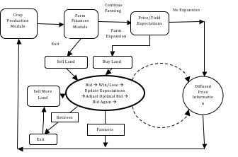
Figure 1. Simulation Flow Diagram - Simulation Modules and Agent Decision Points

2.7

Ultimately, farm agents who meet a specified criterion enter the Auction Module and then bid on plots of land as they become available. This is done until they have purchased all the land that they desire. Once agents are finished with purchases in the auction module, they wait until either; 1) all land is sold, or; 2) there are no bidders remaining. Once the Auction Module is complete, all remaining farmers proceed to the Crop Production Module, starting another simulated crop year where the land purchase cycle starts anew.

The Structure of Farm Agents

2.8

The simulation environment begins with 422 agents. At time t = 0, we randomly assign 97 percent of the agents as Farmer agents, while 3 percent are assigned as Retiree agents. This is an important distinction based on reality. Farmer agents in the simulation are initially endowed with land, machinery and cash, and are assumed to produce crops on their land and sell them at market prices. Behaviorally, we assume that all farmers under age 55 want to expand their farm size by purchasing land from other farmers exiting the market (for simplicity, we also assume that there is no government support for farmers and no off-farm income). Therefore income is generated based solely on a farmer's ability to farm the land successfully.

2.9

Retirees are farmers who have left the industry and want to sell the land they own. If a retiree agent is unsuccessful in selling all plots of land in the first year of retirement, they are assumed to hold on to unsold land. All remaining plots of land go up for sale again in subsequent periods, but at a discounted price. This process continues each simulated year until all plots are sold.

Factors of Farm Production

2.10

Farms in the simulation produce crops using 3 inputs; land, labour, and capital. Different types of farmland are assigned to 1 of the 4225 spaces on the 65 by 65 grid that comprises the virtual farming landscape. Each plot represents one quarter-section or 160 acres. The 422 farmsteads are dispersed randomly over this landscape. Note that plots are heterogeneous in cultivatable acres and quality, but land quality is assumed to be homogeneous within a plot. Each plot has its quality correlated to the plots surrounding it using a relational variable. Plots that are of higher quality (quality > 1) will generate higher yields than plots of lower quality (quality < 1), ceteris paribus. In each period, plots are also randomly assigned a weather variable that affects yields in the same manner as quality. Weather is also assumed to be diffused and correlated across plots.

2.11

As in previous related research, farm agents in the model supply most, but not all, of the required labour for crop production (Freeman et al. 2009). Additional farm labour is purchased on an open market and withdrawals from income are made to compensate farm agents for supplying labour. One of the key components of heterogeneity among farmers will be their productivity measure (skill). For our purposes, we assume that a farmer with higher skill, Sk, is capable of altering crop mixes more effectively so as to extract more output than lesser skilled farmers. Farmers who are more productive (Skill > 1) produce greater yields, and thus more income, than farmers who are less productive (e.g. Skill < 1), ceteris paribus.

2.12

Next, we assume that farm agents are heterogeneous in entrepreneurial attitude, including their risk preferences. Farmers' willingness to assume risk is a function of the assumed goals and objectives for their farm enterprise. Building upon some of the previous research, farms in this simulation operate in one of three distinct life phases of farming: 1) Growth and Expansion, 2) Development, and 3) Maintenance (Freeman et al. 2009)

Crop Production

2.13

Farm agents generate gross farm revenue through the sale of their crops. All farmers produce the same four types of crops, but in different mixes. Crop yields are composed of the weighted average of 4 different crop types. Average yields realized by farmers with the same skill is the same for their given crop mix, ceteris paribus. Diversification of crops is necessary for crop rotational purposes. Total individual crop prices and yields for each farm agent are computed using a weighted average of the crops grown. Equations 1 and 2 below define the relationship between individual prices (yields) and weighted average prices (yields) respectively:

(1)

(2)

where the parameters are non-negative and sum to one.
Both prices, P_i, and average yields, Y_i, are exogenously determined in the simulation. Yields are affected by weather patterns and prices are fixed via a world market assumption.

2.14

Total cost of production for farm agent k consists of fixed and variable costs. Variable costs are a function of area cultivated, yield realized, and distance from plot xy to agent k's farmstead. Farm agents do not decrease variable costs incurred if yield is expected to be poor (Freeman et al. 2009). Fixed costs are constant in year t but can vary across years. They include cost of capital, debt payments, and capital replacement. The management/family living withdrawal is also considered as a fixed cost.

2.15

Variable costs are the sum of all variable costs for all plots of land, i_k=(1_k, …, I_k ) managed by farm agent k in year t. This also includes any non-family labour that is used:

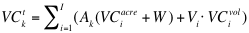
(3)

where A_k is cultivatable acres of farmer k, VC_i^acre is the variable cost per acre of plot i, W is the non-family labour per acre for farmer k, V_i is the production volume for plot I, and VC_i^vol is the variable cost of production for plot i.

2.16

Finally, total fixed cash commitment for a farm operator is defined as:

(4)

where DebtService is the total debt payment in time t, FW_k is the minimum amount of cash that must be withdrawn from farm operation to cover living expenses, managerial costs, and family labour, and FC_k^Capital is the annual reinvestment requirements and is set equal to the economic rate of depreciation.

The Land Market: Farm Exits and Expansion

2.17

We assume that in time t = 0 all farm land is owned. Thus, for any farm agent to purchase land in future time periods, at least one other farm agent must be willing to sell land. Farm agents sell land when they exit the market, and this occurs in the model for one of 3 reasons: Retirement, Forced Exit, or Voluntary Exit.

2.18

Retirement occurs when farmers reach a critical age and no longer wish to farm, while the probability of retirement increases in age. Alternatively, forced exit occurs when a farmer fails a test for financial solvency—when debt exceeds 90% of asset value, the individual is insolvent and forced out of the market. Voluntary exit occurs when a farmer calculates that it is no longer profitable to farm and chooses to exit to protect equity. After retirement or a voluntary exit, farmers can sell their land on the open market or pass it to an heir.

2.19

Land that becomes available for purchase is bid on by farmers who are deemed credit worthy. Credit worthiness is determined by a debt to asset ratio (D/A ratio) criterion, also factoring in a minimum amount of cash necessary to cover down payment and cropping costs for the following year. Farmers are monitored to ensure that expected production margins are sufficient to cover family withdrawals and future debt payments. Expected production margins are calculated as follows (Freeman et al. 2009):

(5)

2.20

Farmers who meet all the criteria can make bids on available land. Farmers who decide to buy (or sell) land need to formulate expectations about future yields and prices to determine the expected profitability of a plot of land. Maximum willingness to pay (WTP) for a plot of land is based on expectations about future yields and prices, and the costs associated with these expectations. Price and yield expectations are formulated as follows:

(6)

(7)

where the parameters are non-negative and sum to one.

2.21

We assume that farmers only have trustworthy yield information for their own crops. As such, the information used by farm agent k will be the average of farm agent k's yields for time periods t - 1 through t - 5 adjusted for average soil quality, and an error ε which is unique to agent k and related to S_k..

Maximum Willingness to Pay, Credit Constraints, and Bid Formation

2.22

Farm agents in the model derive utility from acquiring as much land as possible. Therefore, calculating individual WTP, deciding on an optimal bid, and learning from past experiences are very important. Farm agents only gain advantages over one another via experiences and learned price information. Farmers who make these decisions more often will have more information on which to base future decisions, facilitating more accurate expectation calculations.

2.23

When a buyer calculates maximum WTP, they use their expectations about prices, yields, and the future price of land. Bidding more frequently allows farmers to obtain more accurate information about the expected price of land. Equation 8 illustrates this relationship:

(8)

2.24

Farmers can also be constrained by a maximum borrowing limit. Similar to the actual situation in Western Canadian farming, we assume that farmers make a 25% down payment on any land purchases, meaning that they must borrow 75% of the purchase price from lending institutions. To that end, lending institutions place a maximum borrowing limit on farmers who wish to bid.

2.25

Farmers must determine their valuation for a plot of land. In order to do this, a farm agent relies on prior experience and learned price information. Individual valuation is also influenced by risk preference. A farmer's aversion to losing an auction will be reflected in their valuation of the land. This type of risk is inversely related to expectation risk and is captured by placing upper and lower bounds on a farmer's expected value of land. These are shown in Table 1.

2.26

In this simulation, no single farmer knows the value of a plot of land, and must rely on their learned or updated information to estimate plot value.^[2] Farmers will use learned information to pick a valuation from a distribution of values (Zeng and Sycara 1998). These values are normally distributed around a farmer's learned mean and standard deviation of land prices.

Setting the Reservation Price for Land

2.27

All land that is submitted to auction is assigned a reservation price and listed for sale in each period, until it sells at a price equal to, or above, its reservation price. One can think of farmers who are forced out of the market as having all their assets, including land, repossessed and sold by the bank which subsequently assigns a reservation price. It is important to note that reservation prices are not revealed to potential bidders.

Table 1: Farm Agent Valuation Distributions
Stage	Distribution	Truncation
		Lower Bound	Upper Bound
Growth and Expansion	~N(Est.Mean, Est.Std.Dev)	Mean - (1 Std.Dev)	Mean + (3 Std.Dev)
Development	~N(Est.Mean, Est.Std.Dev)	Mean - (2 Std.Dev)	Mean + (2 Std.Dev)
Maintenance	~N(Est.Mean, Est.Std.Dev)	Mean - (3 Std.Dev)	Mean + (1 Std.Dev)

Source: Authors' calculations.

2.28

Reservation prices are calculated based on a seller's perceived price of land at time t. Perceived prices are a function of learned information about average price per acre. Farm agent k sets:

(9)

where V_k^t is seller k's learned price of land adjusted for acres and quality, and ω is a measure of urgency. In addition, we also assume that retired farmers regularly attend auctions seeking to sell land, meaning that their price information, V_k^t, is at least as accurate as the best informed farmer. As a retiree becomes more determined to sell their land, _ increases, leading to a fall in reserve price. The longer a plot is held for sale without being sold, the higher the seller's urgency.

Prices and Agent Learning

2.29

All farm agents learn over time about the land market, and do so at an equal rate. Agents learn about prices of transacted land parcels, and how to increase 1) the probability of increasing rents when an auction is won, and 2) the probability of winning an auction.

2.30

When agents learn about land markets, they do so via two mechanisms, which we call Local and Global learning. Local learning occurs when an agent participates in an auction - agent k is said to learn locally from auction m when she is a bidder in auction m. Local learning takes place by means of two pathways; 1) Price Information, 2) Optimal Bidding Information. Price information learning means that agents participating in auction m learn the final price (price information) of the plot of land sold in auction m.^[3] This information is perfect and known to all bidders in m. Acquiring optimal bidding information is slightly more difficult and is discussed in detail below.

2.31

Global learning from auction m occurs for all agents who do not take part in auction m. All agents k in K who do not participate in m will receive final price information by means of a diffusion process. Specifically, final price information from auction m will diffuse through the population, getting noisier as the agent's distance from (x,y) increases:

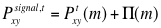
(10)

where P_xy^signal,t is the noisy signal heard by agent k from auction m, P_xy^t is the true final price of plot xy in auction m, Π(m) is the noise term and is η (0,S(m)) and S(m) is increasing in distance from the location of auction m to the farm agent k.

2.32

In this simulation, all farm agents possess a limited memory. They can only hold a finite amount of price and bid information. Once this memory capacity is full, new information replaces the oldest piece of information.

2.33

Finally, the incorporation of Optimal Bidding Information in the simulation is done according to Learning Direction Theory (LDT) (Neugebauer and Selten 2006). LDT is a qualitative behavioural theory motivated by ex post rationality. LDT effectively forces agents to ask themselves whether a different action might have produced a better result. This allows agents to adapt their behaviour by using ex post information on prices to increase their chances of future auction success.^[4]

Auctions and the Revenue Equivalence Theorem: Private, Common, and Affiliated Values

3.1

The revenue equivalence theorem for auctions was first formulated by Vickrey (1961), and later generalized by Myerson (1981). The theorem states that given the following assumptions, particular auctions will yield the same expected seller revenue and allocation of goods:

• Highest bidder wins the auction and receives the good
• Bidders have independent private values drawn from the same, commonly known distribution—values and bids are IID
• Bidders are risk neutral
• Bidders are not budget constrained
• Bidders are perfectly rational and know that all other bidders are also perfectly rational, ad infinitum.

3.2

The revenue equivalence theorem relies on some rather strong assumptions—risk neutrality, IID, perfect information, and homogeneity—in order to ensure that players can find a Nash Equilibrium bidding solution. This last point is particularly important to this research because auction theory has traditionally been examined using Nash Equilibrium bidding functions (Richter 2004). In fact, Vickrey's original work showed that under the assumptions listed above, all private-valued auctions, including the well known English, Dutch, First Price Sealed Bid (FPSB), or Second Price Sealed Bid (SPSB) auctions yield the same expected seller revenue and allocation of goods.

3.3

Vickrey's independent private-values assumption (IID) is the topic of on-going research in auction design. Originally, Vickrey assumed that bidders would value a good independently of how other bidders valued the same good. As mentioned previously, this assumption does not apply to all goods that are sold by auction. In light of this, Wilson (1969) suggested what is known as the common-values approach, which implies that all bidders value a good equally, but its actual value is unknown to all agents. Individual values are therefore based on each agent's best private information about the good. As a result, valuation can differ between agents and is a function of the information available to each agent. The common values assumption is best known for generating the so-called winner's curse situation: in common-value auctions with imperfect information, the winner tends to over pay for the good since the actual value of the good is likely to be closer to the average of all values.

3.4

There is a third type of value model that is commonly used in auction theory, called the affiliated-values model. This uses elements of both private and common values to generate bidder valuations. Milgrom and Weber (1982) proposed this model of competitive bidding because it accounts for personal preferences, preferences of others, and the intrinsic qualities of the item being bid on. Affiliated-values depend on the private information of all bidders; e.g. a high valuation by one bidder makes high valuations by other bidders more likely. Theoretically, this model generates higher selling prices in an English auction than a second-price auction. To date, the majority of analytic auction theory relies on the private-values assumption because common- and affiliated-values models significantly increase the algorithmic complexity of the problem due to the need to capture these interdependencies (Matthews 1987). And very little is understood about the consequences of relying upon common- and affiliated-values assumptions among bidding agents.

Pseudo-Optimal Bidding Mechanisms

3.5

During the course of the simulation we assumed each farm agent acts similarly, regardless of the type of auction mechanism employed to determine their maximum WTP. Beyond this, farmers will formulate bids strategically depending on the type of auction mechanism they will face. Their optimal bidding strategies are founded upon results from the analytic auction literature. The bidding procedure used in the simulation approximates optimal behaviour using known bidding algorithms that are readily computable. Ease of computation is especially important because optimal bidding strategies should be tractable in real world settings.^[5]

3.6

Some other assumptions have been made that are common to all auctions. First, farmers are aware of the number of bidders participating in the auction. Second, if a land auction has only 1 bidder, the transaction converts to a bargaining solution between the bidder and the seller where the final price paid is the mid-point of the bid/ask spread so long as the initial bid is above the reservation price.

3.7

What follows is a description of the auctions and algorithms used by agents to determine their optimal bid based on their WTP: First-Price Sealed Bid (FPSB) Auction. Under a FPSB auction, farmers submit a sealed bid to the auctioneer. After all bids have been received, the auctioneer ranks all bids and awards the plot to the bidder with the highest bid at the price they bid. The optimal bid under certain restrictive assumptions for a FPSB is:

(11)

where X is a farmer's valuation of the plot of land and N is the number of bidders bidding on the plot of land.

Second-Price Sealed Bid (SPSB) Auction. The strategy in a SPSB is similar to that of a FPSB, except that in a SPSB, farmers have the incentive to bid their true valuation, X, for the plot of land (Vickrey 1961). This occurs because the price that the winning farmer pays is not a function of her bid. A winning bidder will pay the second highest bidder's bid, thus, she has no incentive to increase or decrease her bid above or below her true valuation. As such, for the SPSB we have:

(12)

Third-Price Sealed Bid (TPSB) Auction (Kagel and Levin 1993). A TPSB is again similar to the FPSB and SPSB auctions in that it is a single round sealed bid. However, as its name implies, in a TPSB the bidder with the highest bid does not pay their own bid, nor the second highest bid, but the third highest bid. In this case the winning bid will be above X and is decreasing in N:

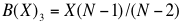
(13)

English Auction. In an English auction, farmers have the ability to make a bid, then re-evaluate their bid based on other farmers' observable bids and submit a new higher bid, if desired. Bidding is divided into 2 rounds. In the first round, all bidders submit oral bids until the bid reaches their personal valuation for the good, B(X). At this point, the bidder with the highest valuation will have submitted a bid equal to the second highest bidder's bid plus a minimum bid increment, ς , and thus would be considered the current winner of the auction.

3.8

After an initial round of bidding, all farm agents are permitted to re-evaluate the common-value element of their bid since more information is available. If they have reason to believe that they have undervalued the land, farmers may choose to submit a new higher bid.

3.9

A farmer will increase their valuation, and bid, for the plot of land to their MaxWTP (if MaxWTP > current highest bid) with some probability ρ. In turn, the probability that a farmer will choose to increase their valuation is dependent on individual risk preferences. Farmers in the Growth and Expansion Phase are more risk averse to losing the auction than a farmer in the Maintenance Phase, meaning the former has a higher probability of increasing valuation to MaxWTP.^[6]

Model Initialization and Data

4.1

Netlogo (V 3.1.5) is the agent-based simulation platform used for this analysis. The NetLogo code can be found in the Appendix to Arsenault's (2007) thesis, while the full working model (Netlogo code including input data used for this study) is also archived on the OpenABM.org website ( http://www.openabm.org/model/2539/version/4/view). Each set of simulation runs begin with similar land market structure. Farm operator attributes include; 1) age, 2) farm size, 3) attitude, 4) financial information, and 5) learned price information, and are homogeneous across iterations. The only factors that change are the location of the farmsteads and the location and quality of the owned plots of land.^[7]

4.2

Farmer age and land area owned (Tables 2 and 3) were compiled by means of a random number generator. Farmer age is distributed η (38.2, 9.32) while land plots owned is η (10.0, 5.94). Initial farm agent assets are equal to the sum of all machinery, land, and cash held at t = 0. Cash accounts are initialized at $75.00 per cultivatable acre while capital stocks, which include machinery, equipment and buildings, are initialized at $100.00 per cultivatable acre. Farm operator debt per acre is distributed as η (101.77, 49.48). This translates to an average farm indebtedness of $165,643. Total farm indebtedness at time t = 0 for all 422 farmers is $69,901,243. Means and standard deviations for all variables were estimated using data from various census agricultural regions in the 2005 Canadian Farm Financial Survey (FFS).

Table 2: Distribution of Initial Plots Owned by Age Group
	Plots Owned (1 Plot = 160 acres)
Age	1 to 5	6 to 10	11 to 15	16 to 20	21 +
20 - 29	15	20	25	17	4
30 - 39	24	52	38	22	10
40 - 49	49	49	37	13	9
50 - 59	9	16	6	0	0
60 - 69	5	2	0	0	0
Source: Authors' calculations based on 2005 FFS.

Table 3: Initial Farmer Debt by Age Group
	Farm Debt (thousands)
Age	<$50	$50 - <$100	$100 - <$300	$300 - <$500	$500 +
20 - 29	13	14	42	10	2
30 - 39	31	19	69	24	3
40 - 49	37	29	65	23	3
50 - 59	7	9	14	1	0
60 - 69	5	2	0	0	0
Source: Authors' calculations based on 2005 FFS.

4.3

The simulation is initialized with 422 farmers with a mean age of 38 and an average farm size of 10 plots (1600 acres). Crop prices and yields used in the simulation are based on price and yield data reported by the government of the province of Saskatchewan for the four crops as grown during the 1985-2004 cropping years.

Measurement and Evaluation

5.1

Allocative Efficiency. For our purposes, an auction is not allocatively efficient if there exists uncertainty in the common-value element of the affiliated-values signal. Due to the nature of the land market, and the ex post realization of value, it is not possible to know if a farm agent's valuation was correct.^[8] Therefore, minimizing variance in auction sale prices has been suggested as one metric of minimized efficiency losses from an allocative standpoint (Goeree and Offerman 2002). To that extent, it is possible to ordinally rank the auctions based on allocative efficiency by measuring price variance in each simulated auction.

5.2

System Surpluses. In the absence of a static equilibrium, it is still possible to measure an agent's perceived surplus from a transaction in this simulation. In this model, transaction surplus is "perceived" because agents do not know with certainty the true value of the land purchased until it is no longer farmed and subsequently sold. Calculations of perceived surplus will be made based on the best information available in the current period -the transacted price for land. To that extent, the auction that generates the most total perceived surplus will be considered the most efficient (Harberger 1971).

5.3

Industry Characteristics and Evolution. A final point of comparison will examine to what extent, if any, choice of auction mechanism has on industry evolution at a macro level. Macro level market characteristics such as farm exits, farm size, financial ratios, and bidder participation will be tracked to determine the impact auction design has on the evolution of this agricultural sector.

Results and Discussion

6.1

What follows is a comparison of eight simulations of farmland market auctions, each run with 100 iterations of 35 years each with Learning Direction Theory (LDT) applied. Summarizing the primary results:

1. The SPSB generated the most perceived total surplus, followed by the TPSB, English, and FPSB auctions respectively (Figure 2).
2. The SPSB and TPSB resulted in the most egalitarian distribution of surplus between the buyer and seller. While potentially important for policy analysis, we draw no conclusions about an "optimal" distribution of surplus in this land auction environment (Figure 3).
3. The English auction generated the most variability in prices. All the sealed-bid auctions performed equally well. This suggests that the common-value elements of the bids in an English auction generate higher price variability than the common-value elements in the sealed-bid auctions.
4. The English auction generated, on average, the highest prices. This was followed by the FPSB, TPSB, and SPSB auctions respectively. The English auction also exaggerated upward trends in sales price more than the sealed-bid auctions.
5. Contrary to our prior expectations, auction choice had no effect on aggregate market characteristics or industry evolution.

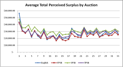
Figure 2. Average Total Perceived Surplus Generated from Sale by Auction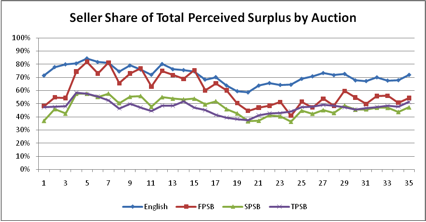

Figure 3. Seller Share of Total Surplus from Sale by Auction

6.2

Learning Direction Theory (LDT). The simulation compared auctions of the same type with and without the imposition of LDT. All four auction types were found to generate greater means and variances when LDT was active. Differences between the means and variances were significant at a 5% level of significance. This result concurs with the work of Neugebauer and Selten (2006) who found that LDT explained, at least in part, some of the over-bidding phenomena observed in repeated auction experiments. However, these findings are somewhat counter to our expectations about the effect of a learning mechanism (that bid variance would decrease under LDT). It is also important to keep in mind that LDT is not so much a true learning mechanism as it is a bid adjustment theory.

6.3

Nevertheless, these findings are unique because much of the existing research about land prices assumes that they are either influenced by speculation, hedonic pricing, capitalization, or expected revenue (Huang et al. 2006). Our results suggest that a non-trivial portion of land prices in modern agriculture could be attributed to a strategic bidding component when there is repeated interaction in land markets.

6.4

Auction Performance. The simulation results also indicate that price level was highest under an English auction, and lowest under the SPSB (Figure 4). Farmland price variance was greatest under the English auction, implying that the English auction may be the least efficient mechanism for land markets. The sealed-bid auctions examined here all performed equally well under this efficiency criteria, implying that uncertainty in common-values might be reduced with the use of sealed-bid auctions, especially when farmland values are assumed to be affiliated in nature (Figure 5).

6.5

Market Characteristics. Simulation results suggest that market evolution is dependent on the rationality of agents. Implicit upper and lower bounds on the price of farmland, coupled agents that are income/productivity driven leads to land markets that track in similar directions in spite of auction choice. That is to say, market characteristics such as participation rates in auctions, financial characteristics, and evolution of market structure were unaffected by auction choice. In sum, our findings imply that so long as the mechanism of choice supports income generating incentives, the system is likely going to be robust to auction or mechanism design.^[9]

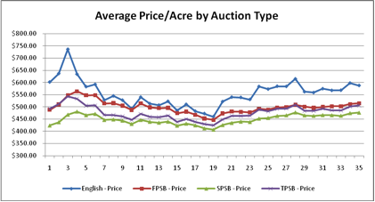
Figure 4. Average Price/Acre by Auction Type with LDT On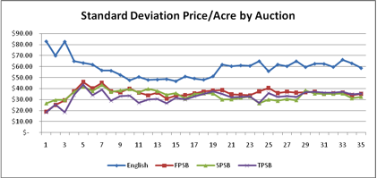

Figure 5. Average Standard Deviation of Price/Acre by Auction Type with LDT On

Conclusions

7.1

The results from this analysis indicate that in the absence of exogenous shocks the farmland auction market seems to be robust to the choice of auction mechanism since each auction type ultimately generated a similar overall land structure. The fact that all auctions produced a similar landscape suggests that even when land bids are sub-optimal, these auction mechanisms can elicit good outcomes provided that the auction mechanism supports income-generating incentives.

7.2

Although our analysis does not permit the identification of the absolute best farmland auction as a one-size-fits-all design, the findings do indicate that the SPSB auction can mitigate overbidding in repeated auctions, yield an equitable distribution of surplus, generate the greatest total surplus as well as send quality signals to other bidders about prices. As usual, these exploratory results should be interpreted with caution. For instance, there are documented real-world instances where SPSB auctions, coupled with weak demand, resulted in market failures by facilitating collusion and subsequent low seller surplus due to lower than predicted transaction prices (Klemplerer 2002).

7.3

Most importantly, the findings must also be viewed in light of the limitations of MAS. The data generated from the MAS is the result of agents acting on the assumptions imposed on them. Although some of these assumptions may not be sufficient to mimic all real world behavior, the flows of information, evolution of time, and the agent landscape have offered valuable insights about farmland auction markets. Multi-agent simulation appears to have the potential to be a valuable tool for future agricultural land market analysis.

Notes

¹To better focus this research on auction choice, we chose not to explore alternative methods of price formulation in farmland markets. See King and Sinden (1994) for a detailed discussion of this issue.

²Learned prices are adjusted to reflect different qualities of land.

³This is true only for auction designs that allow such information. i.e. sealed bid auctions reveal the winning price only, whereas an English auction reveals the bids and the winning price.

⁴A more complete description of LDT as applied in this framework is in Arsenault (2007).

⁵Optimal bidding functions used here are based on established best-response functions from the theoretical auction literature (Kagel and Levin 1993). As noted above, these functions are not optimal in a mathematical sense, but are aligned with incentives that all bidders are assumed to have.

⁶It should be noted that farmers do not change their risk preference, but are more or less likely to change the common-value element of their valuation based on their preferences towards risk, and losing an auction.

⁷Running 100 iterations of each simulation should mitigate any such adverse effects.

⁸Recall that agents form expectations about future prices and yields, and the future price of land. And since the full value of a capital asset (farmland) is based on future income streams, it is not possible for agents to know the true value of any plot of land.

⁹It should be noted that this stylized model does not allow for extreme deviations in prices due to the number of assumptions that are imposed. Allowing for exogenous shocks to the industry may result in shocks to land markets, changing the steady state path.

Acknowledgements

This paper is a product of the unpublished MSc (2007) thesis of A. Arsenault completed at the University of Saskatchewan. The views and opinions expressed herein are those of the authors and do not necessarily reflect the views of Agriculture and Agri-Food Canada, the Minister of Agriculture and Agri-Food Canada, the government of Canada, or its employees. Nolan would also like to thank R. Lawrence for programming assistance in the preparation of this manuscript.

References

ARSENAULT, A. (2007) A Multi-Agent Simulation Approach to Farmland Auction Markets: Repeated Games with Agents that Learn. Unpublished MSc thesis, Dept. of Agricultural Economics, University of Saskatchewan, Saskatoon, SK.

BALMANN, A. (1997) Farm-based Modeling of Regional Structural Change: A Cellular Automata Approach. European Review of Agricultural Economics 24, pp. 85-108. [doi:10.1093/erae/24.1.85]

COLWELL, P.F., Yavas, A. (1994) The Demand for Agricultural Land and Strategic Bidding in Auctions. Journal of Real Estate Finance and Economics 8, pp. 137-149. [doi:10.1007/BF01097034]

FREEMAN, T., J. Nolan and R. Schoney (2009) An Agent-Based Simulation Model of Structural Change in Canadian Prairie Agriculture, 1960-2000. Canadian Journal of Agricultural Economics 57, pp. 537-554. [doi:10.1111/j.1744-7976.2009.01169.x]

GOEREE, J.K., Offerman, T. (2002) Efficiency in Auctions with Private and Common Values: An Experimental Study. The American Economic Review 92, pp. 625-643. [doi:10.1257/00028280260136435]

HARBERGER, A.C. (1971) Three Basic Postulates for Applied Welfare Economics: An Interpretive Essay. Journal of Economic Literature 9, pp. 785-797.

HUANG, H., Miller, G.Y., Sherrick, B.J., Gomez, H.I. (2006) Factors Influencing Illinois Farmland Values. American Journal of Agricultural Economics 88, pp. 459-470. [doi:10.1111/j.1467-8276.2006.00871.x]

KAGEL, J.H. and D. Levin (1993) Auctions: A Survey of Experimental Research. In: Kagel, J.H., Roth, A.E. (eds.) Handbook of Experimental Economics. Princeton University Press, NJ.

KING, J.H. and J.A. Sinden (1994) Price Formation in Farm Land Markets, Land Economics, 70, 38-52. [doi:10.2307/3146439]

KLEMPERER, P. (2002) What Really Matters in Auction Design, Journal of Economic Perspectives 16, pp. 169-189. [doi:10.1257/0895330027166]

MATTHEWS, S. (1987) Comparing Auctions for Risk Averse Buyers: A Buyer's Point of View. Econometrica 55, pp. 633-646. [doi:10.2307/1913603]

MILGROM. P.R., Weber, R.J. (1982) A Theory of Competitive Bidding. Econometrica 50, pp. 1085-1122.

MYERSON, R. (1981) Optimal Auction Design. Mathematics and Operations Research 6, pp. 58-73. [doi:10.1287/moor.6.1.58]

NEUGEBAUER, T., Selten, R. (2006) Individual Behavior of First-Price Auctions: The Importance of Information Feedback in Computerized Experimental Markets. Games and Economic Behavior 54, pp. 183-204. [doi:10.1016/j.geb.2005.10.001]

RICHTER, R. (2004) Revenue Equivalence Revisited: Bounded Rationality in Auctions. Working Paper, University of Kiel. http://www.ecomod.net/conferences/ecomod2004/ecomod2004_papers/80.pdf

VICKREY, W. (1961) Counterspeculation, Auctions, and Competitive Sealed Tenders. Journal of Finance 16, pp. 8-37. [doi:10.1111/j.1540-6261.1961.tb02789.x]

WILSON, R.(1969) Competitive Bidding with Disparate Information. Management Science 15, pp. 446-448. [doi:10.1287/mnsc.15.7.446]

ZENG, D., Sycara, K. (1998) Bayesian Learning in Negotiation. International Journal of Human Computer Studies 48, pp. 125-141. [doi:10.1006/ijhc.1997.0164]