Abstract

To examine the blocking effect of transaction costs on household mobility, we construct a housing consumption model including transaction costs and adopt an analog simulation methodology, analyzing how changes in household income and home prices influence household consumption, savings decisions and the transaction costs blocking effect. We find that changes in housing demand are the fundamental cause of the blocking effect of transaction costs. The more demand changes, the greater the blocking effect is. Besides, increased volatility in home prices worsens the household mobility problem with regards to the blocking effect of transaction costs, while a change in household income does not impact the blocking effect of transaction costs on housing consumption. To expand housing consumption, our findings suggest active measures that should be taken by policymakers to reduce transaction costs and stabilize home prices.

Keywords:

Blocking Effect, Transaction Costs, Housing Consumption, Household Mobility, Simulation Analysis

Introduction

1.1

In a frictionless housing market, households will change residences instantaneously when faced with a change in household size, family income, consumption preferences, and even general home prices. However, in the real world, housing markets are anything but frictionless. For example, household mobility is restricted by the transaction costs involved in compensating real estate agents for their buyer-seller matching services and lenders for arranging new loans. Even search costs, the time and efforts required for the buyer to find a suitable alternative home, must be considered. In China, transaction costs are particularly high leading to a prolonged search process which affects potential buyers' adjustment to their housing consumption according to the changes in their housing demand. Indeed, Zheng (2006) documented that it takes approximately nine months in China for a suitable residence to be selected by a buyer. During this search period, residents remain in their original home causing a severe mismatch between housing demand and consumption, and a resulting sub-optimal utility function.

1.2

Wheaton (1990) reasoned that when a mismatch occurs between households' current home characteristics and their optimal housing consumption, the search for an alternative residence will begin as long as the marginal benefit to finding a more suitable home exceeds the marginal search cost associated with finding the new home. Alternatively stated, when the degree of consumption-demand mismatch exceeds the search costs of finding a new residence, the household will move. Goodman (1990) built a family consumption model to study the influence of transaction costs on housing consumption utility and housing consumption decisions. He adopted a simulation method to quantify the household mobility "blocking effect" of transaction costs. Zhang (2009), Xing (2005), and Lei (2007) also examined the impact of housing transaction costs on a household's consumption utility by introducing transaction costs into household consumption decisions. This article builds a blocking effect model of the transaction costs in the housing market, adopts an analog simulation method to analyze the influence of changes in household income and home prices on housing consumption decisions, and makes policy recommendations to allow for expanding housing consumption.

The blocking effect of transaction costs

Definition of the blocking effect of transaction costs

2.1

When household income, size of the household, and even home prices change, housing demand will no longer match present housing consumption. Importantly, while the drift away from equilibrium on the housing consumption side is often a gradual process, transaction costs associated with changing residences are static and lumpy. For this reason, households do not change residences frequently. They only move when the utility loss caused by the mismatch between housing demand and housing consumption is greater than housing transaction costs. As such, large housing transaction costs delay the process of adjusting housing consumption, leaving families in a disequilibrium state for potentially long periods of time. This phenomenon is termed the "blocking effect" of the transaction costs in the context of this article.

The blocking effect mechanism of transaction costs

2.2

To further analyze the formation of the blocking effect of transaction costs, we divide family consumption into two parts: housing consumption and daily goods consumption, so as to analyze residents' consumption decisions within the context of an income constraint. The household's consumption utility can be represented by a series of indifference curves. When the chosen level of consumption is tangent to the income constraint, consumption utility is maximized. As shown in Figure 1, the solid lines represent the income constraint I and the consumption utility I, respectively. In this figure, the optimal consumption choice is point A, the housing consumption is h₁, and the other daily goods consumption is c₁. When income increases, the income line shifts to the right towards income constraint II, represented by the dotted line. The present household consumption no longer matches current demand, causing a motivation to change consumption. When the influence of transaction costs is not considered, the indifference curve remains tangent to the income constraint, and the point of intersection shifts to the right to point B. When this occurs, housing consumption increases to h₂, and the other daily goods consumption increases to c₂.

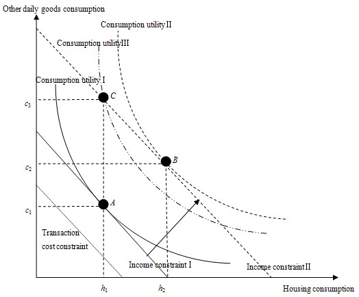
Figure 1. The blocking effect of transaction costs on household consumption decisions

2.3

In the real world, however, when a household moves, transaction costs may exceed several years of the marginal benefit to relocating. When transaction costs are taken into account, the increased income constraint II will shift to the left. If the increase in household income is less than the transaction costs, the real constraint line will shift left, which is even less than the original income constraint I, shown as the transaction costs constraint line in Figure 1. When this occurs, the adjustment of housing consumption lowers total utility, and the household will choose not to move. Instead, they will purchase other daily goods with the same amount of income. The indifference curve intersects the income constraint at point C. The amount of housing consumption is still h ₁, while the amount of other daily goods consumption increases to c ₃. In sum, high transaction costs prevent housing consumption resulting in a mismatch between consumption and demand and a less than optimal level of utility.

Building a blocking effect analysis model of transaction costs

The building principles of the transaction costs blocking effect model

3.1

We adopt an inter-temporal consumption utility model. A household is often faced with two situations with regards to consumption decisions. In the first case, when an increase in income is greater than the transaction costs associated with moving, the households will bear the costs to improve their consumption of housing and other daily goods, and the consumption utility will shift from point A to point B. The housing consumption will increase from h ₁ to h ₂, and other daily goods consumption will increase from c ₁ to c ₂, as shown in Figure 2. In the second case, when an increase in income is less than the transaction costs, the household will choose the same amount of housing consumption, h. When their income grows, the households only improve their daily goods consumption rather than relocating, resulting in a consumption utility shift from point A' to point B'. At this time, although they do not have to bear the transaction costs, the households are indirectly affected by the cost in that they suffer from an increased mismatch between housing demand and housing consumption.

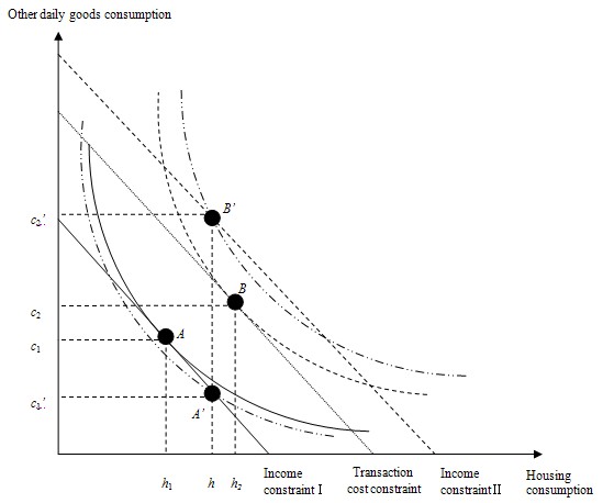
Figure 2. Households' two consumption decisions when affected by transaction costs

Building a housing consumption model excluding transaction costs

3.2

The utility function adopts the classic Cobb-Douglas production function, to maximize the total utility of household consumption. Constrained by the income equation, we can build a basic form of the housing consumption model excluding transaction costs (henceforth referred to as housing consumption model I), shown in equation (1).

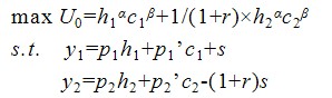
(1)

3.3

In equation (1), U₀ represents the optimal consumption utility without considering transaction costs; α represents the proportion of the housing utility to total utility; β represents the proportion of other consumer goods utility to total utility; r represents the discount rate in one period; y₁ and y₂ represent the consumers' income in the first and second periods, respectively; p₁ and p₂ represent home prices in the first and second periods, respectively; h₁ and h₂ represent the amount of housing consumption in the first and second periods, respectively; p ₁' and p₂' represent the price of other consumer goods in the first and second periods, respectively; c₁ and c₂ represent the amount of other consumer goods consumption in the first and second periods, respectively; and s represents the amount of household savings.

3.4

The housing consumption model is then transformed into a non-linear optimization problem. At the beginning of the first period, the households forecast their income and housing price in the future. Based on their expected income, they will determine the consumption amounts of housing and daily goods in the following two periods and also plan some level of borrowing/lending in order to maximize their long-term consumption utility. When having no constraints on transaction costs, the household will move at the beginning of the second period to meet the new housing demand, causing h₁≠h₂.

Building a housing consumption model including transaction costs

3.5

As described in the basic form of the model, when transaction costs are included, the household is faced with a choice of whether or not to move between the two periods. This decision results in two forms of the model: (1) the housing consumption model not affected by transactions costs versus (2) the housing consumption model affected by transaction costs.

The housing consumption model not affected by transaction costs

3.6

Suppose transaction costs can be accurately anticipated as constant. When households decide to adjust their housing consumption, we experience a housing consumption model that is not affected by transaction costs (henceforth referred to as housing consumption model II), shown in equation (2).

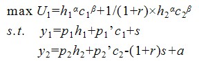
(2)

3.7

In equation (2), U₁ represents the optimal consumption utility when transaction costs are included and housing consumption is not affected by the costs. α represents housing transaction costs.

The housing consumption model affected by transaction costs

3.8

When households choose to remain in the original house, instead of making an adjustment to housing consumption, they only adjust the amount of daily goods consumption at the beginning of the second period. In this situation, h₁= h₂ and c₁≠ c₂. Transaction costs will produce the blocking effect on housing consumption. As a result, the housing consumption model is affected by transaction costs (henceforth referred to as housing consumption model III), shown in equation (3).

(3)

3.9

In equation (3), U ₂ represents the optimal consumption utility when housing consumption is affected by transaction costs; h represents the amount of housing consumption in the first and second periods, respectively.

3.10

When faced with the above two choices, households will compare the long-term expected utilities. When U₁ > U₂, the households will choose to bear the transaction costs and relocate; when U₁ < U₂, they will remain in their original home. In the second case, their housing consumption is blocked by transaction costs. The housing demand does not match their housing consumption, and the households will suffer from housing demand- consumption disequilibrium.

Analog simulation of the housing transaction costs blocking effect model

The first simulation of the transaction costs blocking effect model

4.1

To perform the first simulation, we begin by assigning values to various exogenous market condition variables. Household income in the model can be used for savings, but not entirely for consumption, so we set α+β < 1; here we assume α+β=0.9. Consistent with previous studies, we assume housing consumption utility composes 30% of total consumption utility. Thus we let α=0.27 and β=0.63. We assume a discount rate of 10%. Based on statistics released by the Beijing municipal statistical information website for 2011 coupled with an assumption of dual-income households, average annual household income is set as 100,000 yuan.

4.2

In addition, as the prices of housing and other daily goods merely influence the absolute values of the numerical simulation but have no influence on the changing trend on which we focus, in order to simplify the calculations, we assume the price of other daily goods remains constant at 10,000 yuan. The housing price in the first period is assumed to be 10,000 yuan; the housing price in the second period changes on the basis of that in the first period. If the amount of housing consumption, h, is calculated to be 50, it indicates that 50 units (ten thousand yuan) of housing services will be consumed. The first simulation results are shown in Table 1.

Table 1: First simulation results of the transaction costs blocking effect model
Housing price ratio p2 /p1	Without considering the blocking effect of transaction costs	Without considering the blocking effect of transaction costs	Without considering the blocking effect of transaction costs	Considering the blocking effect of transaction costs	Considering the blocking effect of transaction costs	Considering the blocking effect of transaction costs	Considering the blocking effect of transaction costs
	Housing consumption in the first period(h1)	Housing consumption in the second period (h2)	Household savings(s)	Housing consumption(h)	Household savings(s)	Transaction costs(a)	Proportion of the transaction costs to housing consumption
1.0	30.00	30.00	0.00	30.00	0.00	0.00	0.00%

4.3

According to Table 1, when both home prices and income in the two periods remain the same, without considering transaction costs, if housing demand remains constant, the household chooses to spend 30 units on housing consumption, but not on savings. The optimized choice is then not to adjust housing consumption. Hence, the highest acceptable transaction cost is 0. This shows that the change in housing demand is the key trigger in causing the blocking effect of transaction costs. The households do not have the motivation to relocate when their demand remains constant and as such, they will not be impacted by the blocking effect.

Analysis of the simulation results of the transaction costs blocking effect model

4.4

To compare the influence that changes in household income and home prices have on family consumption decisions, we assume the total household income in the first period remains at 1 million yuan throughout the simulation process and that family income in the second period is 0.5 million yuan, 1 million yuan, 1.5 million yuan and 2 million yuan, respectively, or y₂=0.5 y₁, y₂= y₁, y₂=1.5 y₁, and y₂=2 y₁. We assume the home price in the first period is constant at 10,000 yuan and the fluctuation in home prices in the second period ranges from 5,000 yuan to 20,000 yuan, with the fluctuation rate being 5,000 yuan per unit of time. Then, at the following four levels of income shown in Table 2, we can determine what influences the change in the expected home price has on the simulation results.

Table 2: Influences on the simulation results of the model when family income and home price change at the same time
Housing price ratio p2/p1	Income ratio y2/y1	Without considering the blocking effect of transaction costs			Considering the blocking effect of transaction costs
		Housing consumption in the first period (h1)	Housing consumption in the second period (h2)	Household savings (s)	Housing consumption (h)	Household savings(s)	Transaction costs (a)	Blocking effect of the transaction costs
0.5	0.5	6.32	82.10	78.94	30.00	16.67	9.37	22.81%
	1.0	8.29	107.76	72.36	39.37	-9.37	12.29	22.81%
	1.5	10.27	133.41	65.78	48.75	-35.42	15.22	22.81%
	2.0	12.24	159.07	59.20	58.12	-61.46	18.15	22.81%
1.0	0.5	22.86	22.86	23.81	22.86	23.81	0.00	0.00%
	1.0	30.00	30.00	0.00	30.00	0.00	0.00	0.00%
	1.5	37.14	37.14	-23.81	37.14	-23.81	0.00	0.00%
	2.0	44.29	44.29	-47.62	44.29	-47.62	0.00	0.00%
1.5	0.5	33.46	7.46	-11.53	18.46	28.21	3.36	30.00%
	1.0	43.91	9.80	-46.38	24.23	5.77	4.41	30.00%
	1.5	54.37	12.13	-81.23	30.00	-16.67	5.46	30.00%
	2.0	64.83	14.46	-116.08	35.77	-39.10	6.51	30.00%
2.0	0.5	38.28	2.95	-27.60	15.48	31.18	8.04	136.43%
	1.0	50.24	3.87	-67.48	20.32	9.68	10.55	136.43%
	1.5	62.21	4.79	-107.35	25.16	-11.83	13.06	136.43%
	2.0	74.17	5.71	-147.23	30.00	-33.33	15.57	136.43%

4.5

According to Table 2, across various home price ratios, household consumption decisions change with expected income, which demonstrates almost the same tendency. In general, housing consumption increases with the growth of the future income, while the amount of savings decreases with the growth of future income. Specifically, if we assume both the income ratio and home price ratio to be 0.5, without considering transaction costs, the optimal decision for the family is 6.32 units of housing consumption in the first period, 82.10 units in the second period, and savings of 78.94 units. Because households expect both the future income and home prices to decrease precipitously, they choose to delay the consumption and reduce current expenses in order to increase the amount of future consumption. In this case, if blocked by the transaction costs, the households will not move during the two periods and will spend 30 units of housing consumption and 16.67 units of savings, which is much less than the amount of savings when they are not blocked by transaction costs. As a result, transaction costs compose 22.81% of housing consumption. In addition, when considering transaction costs and a fixed housing price ratio, no matter how much the income ratio changes, the proportion of transaction costs to housing consumption remains constant. Alternatively stated, the change in expected income influences the absolute value of the transaction costs rather than the blocking effect the transaction costs have on housing consumption. This blocking effect is only affected by one factor: the expected price. Moreover, when the expected home price ratio is 1, the blocking effect of transaction costs on housing consumption is 0. Therefore, if we can maintain relatively stable home prices, the influence of transaction costs on housing consumption will be correspondingly reduced.

4.6

To analyze the influence that changes in home price and household income have on consumption decisions, we construct the following graphs which show that the amount of housing consumption and the sum of savings vary with prices at different levels of income (see Figures 3-8).

Influence of changes in household income and home prices on housing consumption decisions

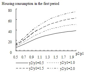
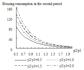
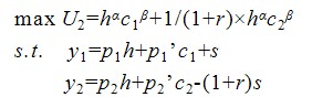
Figure 3. Influence of home prices on households' consumption in the first period at different income levels (without transaction costs)	Figure 4. Influence of home prices on households' consumption in the second period at different income levels (without transaction costs)

4.7

As shown in Figures 3 and 4, without transaction costs, housing consumption in the first period has positive correlations with the expected income and expected home prices in the second period. The housing consumption in the second period has a positive correlation with expected income and a negative correlation with expected home price. In addition, we can see when expected future home prices increase, the elasticity of housing consumption to housing price decreases. Finally, when we observe the distances between curves, we conclude that with an increase in future home prices, the distance between the housing consumption curves in the first period becomes increasingly larger, while that in the second period is significantly decreasing. This shows that as expected future home prices increase, the elasticity of current housing consumption to income increases, while the elasticity of future housing consumption to income decreases.

Figure 5. Influence of home prices on households' consumption decisions at different income levels (affected by the blocking effect)

4.8

According to Figure 5, when housing consumption is blocked by transaction costs, and the household remains in the same home in both periods, as expected future home price increases, the amount of housing consumption will gradually decrease, and the elasticity of housing consumption to home price will diminish. In addition, the distances between the curves do not change drastically; instead, they decrease slightly with the increase in the home price ratio. This indicates that when housing consumption is blocked, an increase in expected home prices causes the elasticity of housing consumption to income to slightly decrease.

Influence of household income and home prices changes on the amount of savings and borrowing

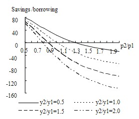
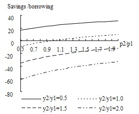
Figure 6. Influence of home prices on households saving decisions at different income levels (without transaction costs)	Figure 7. Influence of home prices on households saving decisions at different income levels (affected by the blocking effect)

4.9

As shown in Figures 6 and 7, without considering transaction costs, the amount of household savings is negatively correlated with home price ratio. With an increase in the home price ratio, a households' savings/borrowing tendency gradually shifts from savings to borrowing. When household mobility is blocked by transaction costs, the amount of savings is positively correlated with home price ratio. The households' savings/borrowing tendency gradually shifts from borrowing to savings, and the slope of the curve changes only slightly. Comparing the curves associated with different income ratios, we can see that the higher the expected future income, the stronger the households' borrowing tendency. Without considering transaction costs, the distances between the curves gradually decrease, which indicates that with the increase in expected future home prices, the elasticity of household savings to income decreases. When the household is blocked by transaction costs, the distances betwesen the curves change very little, indicating that with the increase in expected home prices, the elasticity of household savings to income almost remains constant.

Influence of changes in household income and home prices on transaction costs and the blocking effect

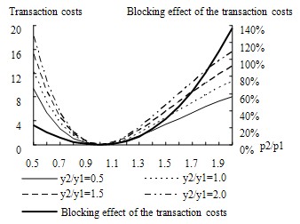
Figure 8. Influence of home prices on transaction costs and the blocking effect at different income levels

4.10

As shown in Figure 8, when the home price ratio is less than one, the highest acceptable transaction costs associated with different income ratios all negatively correlate with home price ratios, and the slope is larger. When the home price ratio is greater than one, the highest acceptable transaction costs associated with different income ratios all positively correlate with home price ratios, and the slope is relatively small. This indicates that when expected future home prices increase, the elasticity of the absolute value of transaction costs to the home price is relatively small. Comparing the curves associated with different income ratios, we can see that the higher the expected future income, the larger the highest acceptable transaction costs, and the larger the slope, or the larger the elasticity of the transaction costs to price.

4.11

The proportion of the transaction costs to housing consumption does not vary with expected income. Therefore, the increase in expected household income only raises the absolute value of the transaction costs, but does not affect the blocking effect on housing consumption. The blocking effect is only related to expected future home prices. When expected future home prices decrease, the blocking effect will decrease with the increase in expected price, with a slow changing rate, and a small elasticity. When expected future home prices increase, the blocking effect will increase with the increase in expected price, with a quickly changing rate and an increasingly large elasticity.

Conclusions and suggestions

5.1

Referring to the Cobb-Douglas production function, this article builds an inter-temporal housing consumption model including transaction costs, and analyzes how changes in household income and home prices influence household consumption, savings decisions and the transaction costs blocking effect. We find: (1) increased volatility in home prices worsens the household mobility problem with regards to the blocking effect of transaction costs; (2) a change in household income does not impact the blocking effect of transaction costs on housing consumption; (3) when transaction costs are excessive, only a significant change in housing demand will cause a household to relocate. These findings underscore the importance of home price stability and reduced transaction costs in residential real estate if policymakers hope to encourage home ownership and maximize the efficient allocation of resources in the housing market.

Acknowledgements

This work was funded by the National Natural Science Foundation of China (No.71073096).

References

GOODMAN, A. C. (1990). Modeling and Computing Transactions Costs for Purchasers of Housing Services. Journal of the American Real Estate & Urban Economics Association, 18(1), 1-21. [doi:10.1111/1540-6229.00506]

LEI, Q. L. (2007). Typical characteristics of family consumption behaviors and optimization analysis of the inter-temporal choices. Consumer Economics, 23(5), 57-60. (in Chinese)

WHEATON, W. C. (1990). Vacancy, search, and price in a housing market matching model. Journal of Political Economy, 98(6), 1270-1292. [doi:10.1086/261734]

XING, Z. L., FAN, A. G. (2005). "Family production function": an expansion of the utility function. Journal of Shijiazhuang University of Economics, 28(3), 346-349. (in Chinese)

ZHANG, X. G., ZHANG, H. (2009). Transaction information costs in Beijing's housing market based on a Hedonic model. Journal of Tsinghua University (Science and Technology), 49(3), 321-324. (in Chinese)

ZHENG, S. Q. (2006). A Microeconomic Analysis of Housing Demand in China-theory and case. Beijing: China Architecture and Building Press. (in Chinese)