
 Abstract
- Observations in experiments show that players in a prisoner's dilemma may adhere more or less to a cooperative norm. Adherence is defined by the intensity of pro-social emotions, like guilt, of deviating from the norm. Players consider also payoffs from defection as a motive to deviate. By combining both incentives, the modeling may explain conditional cooperation and the existence of polymorphic equilibria in which cooperators and defectors coexist. We then show by the use of simulations, that local interaction structures may produce segregation and the appearance of cooperative zones under these conditions.
- Keywords:
- Social Emotions, Norms, Prisoner, Spatial Interaction Structures, Segregation, Agent-Based Simulation
Introduction
- 1.1
-
Human cooperation is explained by different arguments such as kin selection (Hamilton 1964),
direct reciprocity based on the repetition of the game (Fudenberg & Maskin 1986; Axelrod & Hamilton 1981; Kreps et al. 1982; Trivers 1971)
and indirect reciprocity based on reputation building (Alexander 1987).
Cooperation may also arise in a prisoner's dilemma as an effect of the interaction structure but in conjunction with segregative patterns (Helbing et al. 2011; Nowak & May 1992; Nowak et al. 1994; Epstein 1997; Eshel et al. 1998; Cohen & Riolo 2001). That is, a context preserving social structure is necessary for cooperation to emerge and in contrast, random pairing performs poorly for the survival of cooperation. Whereas, the emergence of cooperation in these spatial models rests on imitation/reproduction of the ''best'' procedure (Eguıluz et al. 2005; Helbing et al. 2011; Nowak & May 1992; Nowak et al. 1994; Eshel et al. 1998),
or biological reproduction of the fittest (Epstein 1997; Cohen & Riolo 2001), our paper uses utility maximizing agents to show that cooperative segregation can appear in the context of spatial games with myopic agents.
- 1.2
-
For this, we extend the prisoner's dilemma to integrate two observations from experimental economics which are conditional cooperation and norm abiding behavior by individuals. That is, our modeling must account for the fact that individuals have different behavior underlying diversity in preferences and interactions based on strong reciprocity (Ledyard 1995; Camerer 2003; Fehr et al. 2002). Notably, conditional cooperation and selfishness are mostly observed in public good games (Fischbacher et al. 2001) and cooperation exists even in one shot games (Ledyard 1995; Camerer & Thaler 1995; Fehr & Gächter 2000). Two types of theories explain the deviation from the selfishness axiom shown by these experimental facts. Social preference models (Fehr & Schmidt 1999; Bolton & Ockenfels 2000) posit that individuals are not only interested in their own earnings but also by the distribution of these earnings. Reciprocal models (Falk & Fischbacher 2006; Rabin 1993; Dufwenberg & Kirchsteiger 2004) posit that individuals incorporate the consequences for others positively or negatively in their preference functions depending on whether others are considered as being nice or mean. Implicitly however, both approaches appeal to some normative judgment in stating what should be fair or kind i.e. an implicit norm is required. Our modeling postulates that individuals adhere more or less to a cooperative norm. Indeed, experiments show that individuals globally adhere to a cooperative norm both in repeated and non repeated interactions although this may depend in a non trivial way on the type of social groups (Henrich et al. 2001; Henrich et al. 2005) and differ across individuals within a group (Winter et al. 2012; Fehr & Fischbacher 2004a). In addition, the possible heterogeneity of behavior and the presence of conditional cooperation is explained in this paper by considering that people have prosocial emotions, here shame or guilt, from deviating from a cooperative norm (Bowles & Gintis 2005) albeit to a different degree 2. In fact, negative emotions toward defectors have been shown to be a proxy mechanism behind altruistic punishment (Fehr & Gächter 2002) and difference in adherence to a norm as a source of potential conflict (Winter et al. 2012). Possible coexistence of cooperators and defectors is then a result of our modeling assumptions, i.e. prosocial emotions and norm abiding behavior, which may thus account for the difference in the types of social groups, some of which are actively cooperating groups, others showing more selfish outcomes (Henrich et al. 2001; Henrich et al. 2005).
- 1.3
-
The modeling also relates to the literature on social interactions, in which actions of a reference group affect the individual's preference (Glaeser & Scheinkman 2000; Glaeser et al. 2003; Brock & Durlauf 2001). In the transformed game including emotions, cooperation may be a best response for some people given the overall cooperating rate of their reference group and their emotional value to conform to the norm. For the type of the reference group, our model explores both issues of random or local (and fixed) interaction structures. Another type of game where the payoff structure implies the coexistence of cooperators and defectors is the snowdrift game (Doebeli & Hauert 2005). However, our payoff structure is different from this game and resembles more to an assurance game at least for some players for which cooperation may be a best response given the cooperation rate in their reference group.
- 1.4
-
In a first section, we frame the model proposed in Gordon et al. (2005) as a bayesian game, where the link between a procosial emotion and a norm is made transparent, and call it a normative game with emotions. In addition, the equilibrium configuration from pairwise encounters from a large population, called the global interaction case, is shown for a uniform distribution. In a second section, we present a simulation model with the aim of studying local or random interaction structures of different size. For each structure of interaction, we show the resulting cooperation, segregation and frustration (unhappiness) levels. In addition, we perform a sensitivity analysis for the major result of the section, i.e., that segregation appears under small local interaction structures depending on the distribution of emotions. The final section concludes.
A normative game with emotions
- 2.1
-
The game is a prisoner's dilemma (PD) where we integrate a cost, interpreted as an emotion, of deviating from a cooperative norm.
Assumption 1 Cooperation is an implicit norm on which all players agree but adherence to the norm depends on an idiosyncratic prosocial emotion called guilt.
- 2.2
-
Taking cooperation as players' implicit norm is a rather ad-hoc assumption favorable to the resolution of the social dilemma but which may be justified by the following reasons. First, in many situations, people know which is the implicit norm to follow simply by cultural or legal prescriptions. Second, observations in experimental games show a tendency for people to cooperate in one shot games. Players in these games seem to understand which should be the expected action from the collective point of view. For example, punishments are most often triggered by deviation from the cooperative norm (Fehr & Fischbacher 2004b). Indeed, recent advances in neuroeconomics have shown that people are wired with social norms of fairness (Tabibnia et al. 2008; Sanfey et al. 2003) or conditional cooperation (Zak 2005). In the words of Zak (2005): ''nature has designed us to be conditional cooperators because it makes us feel good''. Emotions together with reward seeking decisions may thus play a dual role in observed behavior (Tabibnia et al. 2008; Loewenstein et al. 2008). Last, from a modeling point of view, it makes no difference whether we suppose that agents have an implicit cooperative norm but null emotions of deviating from it or do not have a norm of cooperation at all. In both cases, we are back to the PD game for these two types of individuals. That is, supposing that some agents do not have a cooperative norm in mind may simply be interpreted as no adherence to the norm. Indeed, normative conflict can be due to two factors ; either by individuals holding different norms , or by difference in the degree of commitment, i.e. adherence, to the same norm. Winter et al. (2012) show that both may explain experimental data in an ultimatum game.
- 2.3
-
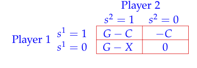
The modeling supposes that there is a population of N agents. In each period, two randomly chosen individuals from a large population are matched together to play the game in table 1.
- 2.4
-
Each individual has a private gain G > 0 if the other individual cooperates. The cooperation cost is C with 0 < C < G. Since cooperation benefits only to the other individual but is socially optimal (G - C > 0), we have a social dilemma. The game with no emotional cost X is a PD game and represents the real payoff of the game. We will refer to real payoff as fitness in the following. In addition, each player i has a type Xi which is private information to him and represents the guilt/shame of deviating from cooperation. For each i, Xi is an identical and independent realization from a continuous and strictly increasing probability distribution F(x) on [0, XM]. F(x) is common knowledge. A free rider (si = 0) does not support the cost of cooperation but supports its emotional cost Xi whenever faced with a cooperator. A pure strategy for an agent is a function s(Xi) from [0, XM] into
Si =
 0, 1
0, 1 . The utility function of individual i can be written as:
- 2.5
-
We define a normative game with emotions to be a Bayesian game Gb = (N,(Si)iwith the additional feature that emotions which represent agents' types are triggered by deviation from a specified profile of actions (
 N,(Xi)i N, F,(ui)i N,(
 )i N)
)i N)
 )i N (the implicit norm).
N is the set of players, (Xi)i N players' types, F the cumulative distribution of players' types,
(Si)i N a set of actions. What is added to a standard Bayesian game is the specification of an implicit norm referring to a specific course of actions supposed to be wired in players' mind which makes clear the dual link between social emotions and norms. A type of an agent is given by the emotional feeling triggered when deviating from the implicit norm. We take the implicit norm to be s = 1 i.e. cooperation. Note that a player with Xi = 0 has a dominant strategy and will always defect.
Let be the probability that sj = 1. Let
Xc(j) = C / . A player i's best response depends on Xc(j) which is a function of the probability that player j cooperates as well as the size of the cooperation cost.
be the probability that sj = 1. Let
Xc(j) = C / . A player i's best response depends on Xc(j) which is a function of the probability that player j cooperates as well as the size of the cooperation cost.
- 2.6
- The best response function of player i is given by:
- 2.7
- In deciding whether to cooperate or not, a player compares two costs: the cost of cooperation C and the expected player's emotional cost of facing a cooperator
Xi. If
C > Xi then cooperation is costly compared to the emotional cost and defection is optimal. Otherwise, cooperation is better. Note than when = 0 then
 = 0 is the best response of player i whatever Xi. And given that
= 0,
= 0 is a best response for player j. Defection, that is
= 0 is the best response of player i whatever Xi. And given that
= 0,
= 0 is a best response for player j. Defection, that is  = 0, is always an equilibrium. Moreover, the size of G ( > C) plays no role in the determination of the Nash equilibria.
A Bayesian equilibrium is a pair of strategies (si*(.), sj*(.)) such that for each player i and every possible value Xi , the strategy si*(Xi) maximizes Eui(si, sj*(Xj)| Xi).- 2.8
- Let Y = X / XM be a normalized random variable on [0, 1] with distribution F1(Y). Denote G1(X) = 1 - F1(X). We have the following characterization of a Bayesian Nash equilibrium: Proof: by equations 2a ,
 = 0 if
 Xi < C and similar for player j. Player's j best response to
= 0 is
= 0 which implies that
= 0. Suppose an equilibrium with
> 0. A player i cooperates with positive probability if Xi belong to
[Xc, XM] by 2b and 2c which occurs with probability
1 - F(Xc) i.e.
= G1
Xi < C and similar for player j. Player's j best response to
= 0 is
= 0 which implies that
= 0. Suppose an equilibrium with
> 0. A player i cooperates with positive probability if Xi belong to
[Xc, XM] by 2b and 2c which occurs with probability
1 - F(Xc) i.e.
= G1 C/XM
C/XM . In a symmetric equilibrium,
= G1(C/XM). QED
. In a symmetric equilibrium,
= G1(C/XM). QED
A necessary condition for the existence of an equilibrium with cooperation is C < XM since Xi must be greater than Xc.- 2.9
- We can also interpret the game as a population game with utility defined by equation 1. With a proportion
of cooperators the average utility of individual i playing against the field is:
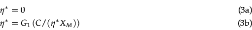
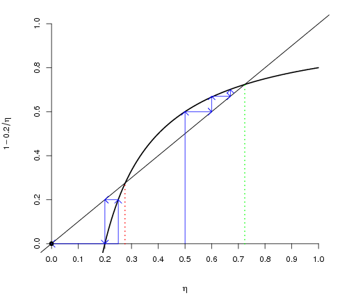
For a large population, depending on the parameters C and F(.), a polymorphic equilibrium exists with coexistence of cooperators and free riders given by equation 3b as shown in Gordon et al. (2005).- 2.10
- The next section contains simulation results when interactions are restricted to a limited number of neighbors. Payoffs are given by the average utility against the players who are part of the interaction structure. As already noted, Nash equilibrium analysis is independent by a normalization of all variables by XM. In performing simulations, individual emotions will then be a N-sample from a uniform distribution on [0, 1]. Defining c = C/XM, the equilibrium configuration for a uniform distribution with cooperation is given by
 = (1 -
  )
)(5)
and has two fixed points given by
with D = 1 - 4c and c 1/4 for such an equilibrium to exist.
The only stable equilibrium with cooperation under global interaction corresponds to
* =
1/4 for such an equilibrium to exist.
The only stable equilibrium with cooperation under global interaction corresponds to
* =  with a basin of attraction given by
>
with a basin of attraction given by
>  . The other stable equilibrium is with full defection i.e. * = 0.
- 2.11
- Figure 1 shows the equilibria and convergence under Cournot best response dynamics. The next section presents simulation results with the following parameters setting: XM = 1, C = 0.2, G = 1 for a uniform distribution. For these parameters, the equilibrium under global interaction depends on the initial proportion of cooperators. With less than 27.6 percent of initial cooperators, convergence under Cournot best response is to pure defection; otherwise, an equilibrium with 72.4 percent of cooperators is expected with coexistence of pure free riders and conditional cooperators. Figure 1 pictures the equilibria. Remember that pure free riders have Xi < C that is, whatever the proportion of cooperators, free riding is optimal. Other individuals are conditional cooperators who cooperate depending on the actual proportion of cooperators.
![\begin{subequations}\begin{gather}\text{if } X^i<X_c(j) \Rightarrow \eta^i = 0\\...
...ht]\\ \text{if } X^i>X_c(j) \Rightarrow \eta^i = 1\end{gather}\end{subequations}](14/img9.png)

Interactions structures and segregated cooperation
-
A first case study with the uniform distribution
- 3.1
-
In this section, we are interested in the study of patterns of cooperation and segregation in a highly stylized situation where agents interact with a small number of other agents. Indeed our interest is to show that segregation may appear from the structure of interactions, implying different patterns of cooperation in comparison to the global interaction case. For this sake, agent-based modeling is a useful tool.
- 3.2
-
In each period t, a random sample of n < N agents play the normative game with emotions with payoffs given by equation 4. Each of them, say individual i, draws a sample of k other players and chooses a stochastic best response to
 (t - 1) where
(t - 1) is the proportion of players playing s = 1 in player's i sample in period (t - 1). By a stochastic best response, we mean that the strategy is randomly chosen with a probability
(t - 1) where
(t - 1) is the proportion of players playing s = 1 in player's i sample in period (t - 1). By a stochastic best response, we mean that the strategy is randomly chosen with a probability  or is a best response to the proportion
with a probability
1 - .
The neighborhood is either local (fixed k nearest neighbors on the lattice) or random (k randomly chosen players from the population in each period). The neighborhood sample size is taken to be one of
k = 4, 8, 24, 44 from a population of N = 100 agents.3 At time t, we define the state of the system by a N-tuple
s(t) =
or is a best response to the proportion
with a probability
1 - .
The neighborhood is either local (fixed k nearest neighbors on the lattice) or random (k randomly chosen players from the population in each period). The neighborhood sample size is taken to be one of
k = 4, 8, 24, 44 from a population of N = 100 agents.3 At time t, we define the state of the system by a N-tuple
s(t) =  s1(t), s2(t),..., sN(t)
 SN = 0, 1
 . Note that since only n ( < N) players are active in each period, passive players stick to their last played strategy. It means that each period only n items of the state space are updated.
- 3.3
-
As an illustrative case, we present simulation results for a uniform distribution and parameters: XM = 1, C = 0.2, G = 1, n = 5,
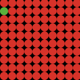
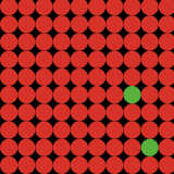
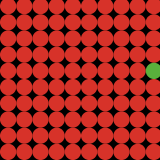
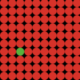
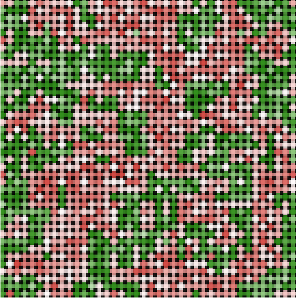
= 2. As noted, for XM = 1, C = 0.2, G = 1, an equilibrium with coexistence of cooperators and defectors exists and may be attained depending on the initial proportion of cooperators (fig 1). Figure 2 shows a snapshot representing the state space of cooperators and defectors after 3000 time periods for each interaction structure. Initialization of the state space is identical for each interaction structure and is such that the initial proportion of cooperation is 20 percent and the mean emotional level in the population is 0, 5016. In this case, full defection is predicted at equilibrium under a Cournot best response dynamics. Unexpectedly, the figure shows a positive cooperation rate for a sample size of 4. Indeed, for a sample size of k = 24 or k = 44, we have full defection (up to noisy cooperation) as expected in equilibrium. This will be a general result shown in the following: local interaction with a small sample size produces cooperative zones different from the global equilibrium prediction. Moreover, cooperation is persistent and segregated with local interactions whereas it is not for random interaction configurations. Localized interactions in small groups may be a factor explaining cooperative segregation as shown in the following paragraph.
Figure 2: State space for different interaction structures. Initial parameters: cooperation 20%, mean emotion 0, 5016. Expected equilibrium at 0 . Red (darker) spots are defectors; green (lighter) spots are cooperators. For k = 24 and 44, we have full defection except some noisy cooperation. World is a torus. Size 4 Size 8 Size 24 Size 44 LOCAL 


RANDOM 
Generalisation
- 3.4
-
We run 32 simulations for each interaction structure with the following parameter configurations: at each time period t, n = 5 randomly chosen players play a stochastic best response (
= 2 percent) to a sample from the state space SN(t - 1); the total number of periods is T = 3000.4
The use of some randomness, i.e.
= 2, allows to check the robustness of the results to small perturbations. We control for initial conditions, i.e. agents' emotions and initial actions, by taking the same initial seed for each different interaction structure. Thus for a given seed, we perform a run for each interaction structure that is, L4, L8, L24, R4, R8, R24 corresponding to local (L) versus random (R) interactions for the different sample size levels
k = 4, 8, 24. More common names for local interaction neighborhoods are Von Neumann for L4, Moore for L8, Moore with range 2 for L24 and Moore with range 3 for L44. Roughly under global interaction, half of the 32 runs predicted full defection given the initial conditions and the other half, high cooperation.
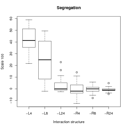
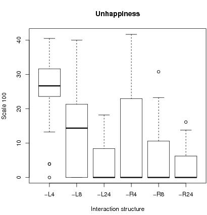
Figure 3: For each interaction structure, the lower bound (whisker line), 1st quartile (hinge), median, 3rd quartile (hinge) and upper bound (whisker line) are shown. The Whisker lines indicate the smallest and largest observation falling within a distance of 1.5 the box size from the nearest hinge. Unusual observations fall outside this range and are represented by a circle. 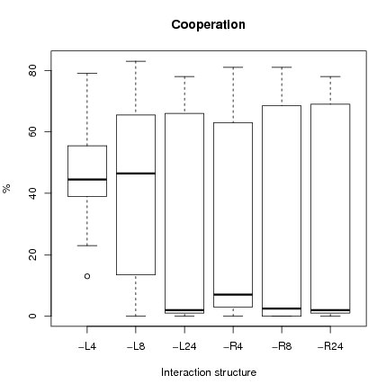
- 3.5
-
Figure 3 shows a box plot for the
32×6 runs (and table 3 in the appendix for rough data). Median cooperation is higher and cooperation is less dispersed under local interactions with small sample size (L4 and L8) than with any other interaction configuration.
There is no equilibrium with full defection equilibrium for the case L4. For L4, and to a lesser degree L8, the impact of the initial number of cooperators is less important than for other configurations where more dispersion in cooperation is observed. This is confirmed by a Chi-2 test on a restricted parameter configuration set. We check whether starting from an initial basin of attraction favorable to one of the two equilibria, we stay in the basin of attraction of the equilibrium by period 3000 (H0 hypothesis) 5.
- 3.6
-
Indeed for initial conditions where an equilibrium of full defection is expected, H0 is rejected for L4 and L8 (p-values < 0.05). That is starting from an initial cooperation rate below 27, the final cooperation rate is above 27. For configurations R24 and L24, the level of cooperation was near to zero in all cases which, given the stochastic best response indicates convergence to the low equilibrium. The same procedure is applied to runs favorable to the high equilibrium. H0 is rejected only for R4 and R8 (p-values less than 0.05) that is starting from an initial condition with a cooperation rate greater than 27, the final state of cooperation is less than 27. The principal conclusion is first, that L4 and L8 lead to a high cooperation level independently of the initial cooperation rate and second, that L24 and R24 never reject H0 and therefore conform to the global equilibrium analysis.
Segregation and fitness
- 3.7
-
We define a normalized index of segregation taking into account the fact that the proportion of cooperators changes during a run. We do that in the spirit of Carrington & Troske (1997). A natural measure of non segregation would be a function
 defined as the sum over all agents of the number of defector-cooperator pairs in a local neighbourhood of sample size k. The higher this index the lower the segregation. Since k and vary across and within a run, we need to define a unit free measure of segregation. Segregation arising by randomness with same parameters k and should not be considered as real segregation.
A random configuration with parameters k, and population size N would give an expected value of
E() = k**(1 - )*N of mixed pairs so that a normalized degree of segregation is
defined as the sum over all agents of the number of defector-cooperator pairs in a local neighbourhood of sample size k. The higher this index the lower the segregation. Since k and vary across and within a run, we need to define a unit free measure of segregation. Segregation arising by randomness with same parameters k and should not be considered as real segregation.
A random configuration with parameters k, and population size N would give an expected value of
E() = k**(1 - )*N of mixed pairs so that a normalized degree of segregation is
 =
=  . If
is around zero then segregation is not different from the one arising in a random configuration. Higher values of
correspond to higher levels of segregation
6.
. If
is around zero then segregation is not different from the one arising in a random configuration. Higher values of
correspond to higher levels of segregation
6.
- 3.8
-
The left figure 4 shows a box plot of segregation depending on the type of interactions. First, one observes that fixed local interactions with small sample size k = 4, 8 lead to higher segregation than with other interaction structures. Remembering that these are also the cases where cooperation is persistent, we have the paradoxical effect that local interactions with small sample size lead to robust cooperation with segregation. Indeed, it is segregation which supports localized cooperation much in the spirit of Epstein (1997) and Cohen & Riolo (2001), albeit with a different kind of rationality. Second for L24 and R24, we know from the preceding paragraph that cooperation is consistent with global equilibrium analysis. Since in this case, cooperation depends on the initial distribution of emotions among the N individuals on the lattice which indeed are obtained randomly, segregation will be low. Last, with random interactions, cooperation depends on the chosen sample and the emotions of the moving players. Since sampling is completely random, segregation must be low.
In addition, we define an index of unhappiness as the proportion of defectors who would like to cooperate given their idiosyncratic emotions and the overall cooperation rate. Unhappiness is linked to segregation and cooperation. Since local interactions with small sample size lead to segregation and significant cooperation, some people will find themselves prisoners of zones of defection and be frustrated. The right figure 4 shows that indeed dissatisfaction is highest with L4 and L8. This shows that local interactions with small samples lead to a situation where people may become frustrated in their environment.
Figure 5: Boxplot of fitness differential (left fig) and average fitness with standard deviation (right fig. on a scale 100). 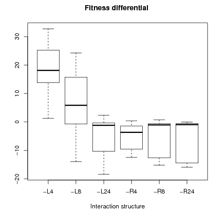
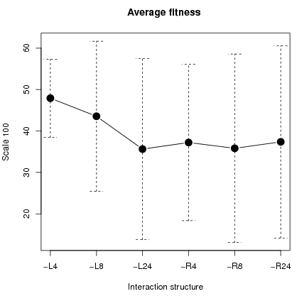
- 3.9
-
Concerning fitness, we compute the differential in fitness between cooperators and defectors. Left figure 5 shows that cooperators are better off than defectors with localized interactions. Fitness is defined as ''real'' payoffs, i.e. emotions are not considered. Fitness corresponds thus to the payoff in a PD game7. Only for L4 and L8 are cooperators better off than defectors as shown in the left figure 5. For L4, cooperators always earned more than defectors. Overall mean fitness was higher in configurations L4 and L8 as shown in right figure 5.
- 3.10
-
As a preliminary conclusion:
- Cooperation is resilient with small localized interactions.
- For the given stochastic best response function, large sample interactions lead to predictions which are conform to the global analysis.
- Cooperators are preserved from defectors in local interactions with small sample size due to high segregation, although some players with high emotions may be trapped in defection zones and become frustrated. Thus, if cooperation is resilient with small local interactions, it will be at a lower level.
Sensitivity analysis
- 3.11
-
The essential question about generalizing the results is whether segregated cooperation under local interactions is preserved by varying parameters of error size, number of periods and number of "moving" individuals n.8 Population size, the distribution of emotions and the cost of cooperation will be considered subsequently. Note that if segregated cooperation is preserved, then the by-side effects of frustration and preserved earnings by cooperators will be valid.
We treat here different issues concerning the validity of our results with different parameters. With respect to the initial parameter configuration of the preceding paragraph T = 3000 ,
= 2 (error) and n = 5 (number of agents playing in each period), we make the following changes:
- varying error size;
= 0, 2, 10 (T=25000; n= 5; N=100)
- varying simulation length T: T= 3000 versus T= 25000 ( = 2; n = 5 , N=100)
- varying n; n = 5, 1 20 (T= 25000 , = 2, N=100)
- varying error size;
- 3.12
-
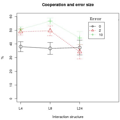
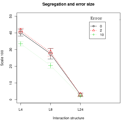
The first result is that the error size affects the cooperation level. Left figure 6 shows that higher cooperation is obtained in the case of small error sizes (2 or 10) compared to no error for small interaction structures (L4 and L8). In contrast, for the larger interaction structure L24, zero error produces no statistical difference in mean cooperation with error 2 or 10 (only error sizes 2 and 10 show a difference in mean cooperation, t-test with a p-value of 0.0172). In addition, the conclusion that segregation is resilient with small localized interactions is true for all error levels (right fig. 6).
Figure 7: Left plot: Impact of time on segregation. Right plot: Impact of the number of moving agent . All plots with 95% confidence intervals . 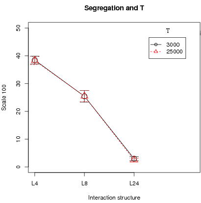
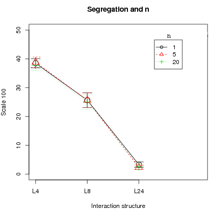
- 3.13
-
Second, the number of period T plays no essential role since there is no difference in cooperation and segregation, averaged over the different runs, between T = 3000 and T = 25000 (left fig. 7, only segregation shown). Cooperation and segregation is still the highest with L4 and L8. Indeed, cooperation has stabilized by T = 3000 and once stabilized, it remains there. Last, the number of active players n makes no difference in the results of cooperation and segregation (right fig. 7, only segregation shown). In addition, synchronous updating, i.e. when all agents are active (n = N), was tested with N = 100 and N = 400 and the conclusions of segregated cooperation with higher fitness for cooperators under L4 and L8 hold under synchronous updating.
Impact ot the population size
- 3.14
-
One additional question is whether the population size N plays a role in segregation.
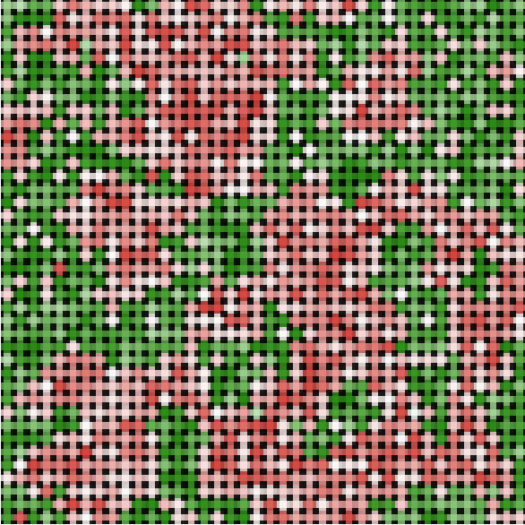
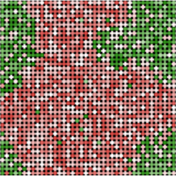
Snapshots in figure 8 show that this may indeed be the case. Starting with an overall cooperation rate of 24.9% and mean emotions in the population equal to 0.5004, the final pattern shows segregation occurring for all structures of local interactions L4, L8, L24 and L44.
Cooperative zones emerge by the existence of clusters of high emotional agents as shown in figure 8. In this figure, the darker a cell is, the larger an agent's emotion is. Indeed a larger neighborhood size may have a positive effect for high emotional agents trapped in defection zones when interaction structures are L4 or L8. For example the top right corner of snapshot L4 of the figure 8 shows high emotional agents who defect (darker red cells) while these agents cooperates for interaction structure L24 and L44.
Figure 8: Snapshots for population size 1600: initial setting 24.9% cooperators. Parameters : n = 5 , = 2, T = 10000, mean emotion = 0.5004. The lighter a cell, the lower an agent's emotion is. The world is a torus.Initial Setting L4 L8 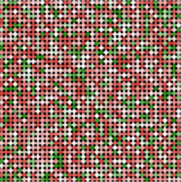
L24 L44 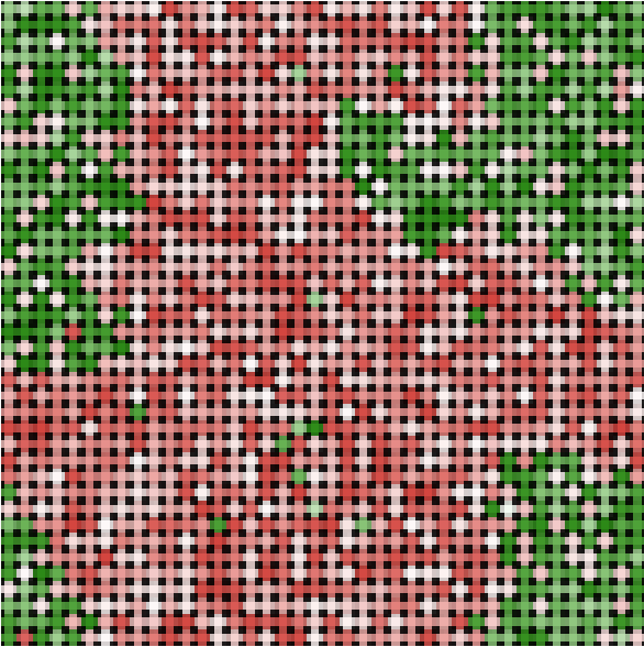
- 3.15
-
We performed additional 30 runs for each of five different population sizes: N = 100, 225, 400, 900, 1600 and each interaction structure. Other parameters are set to : error size = 2, T = 25000, n = 5 and memory = 50.10 We included sample size 44 (L44).
- 3.16
-
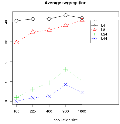
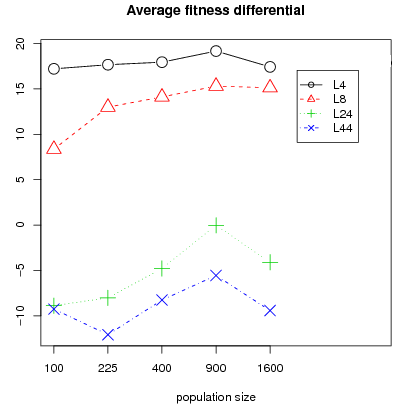
Figure 9 shows average segregation and average fitness differential over the 30 runs for different population sizes. A Fligner Policelli test11 shows that for the interaction structure L4, segregation is identical for different population size (at any level of significance), and for L8, L24, L44 segregation is higher for population size 900 and 1600 when compared to population size 100 (p-values less than or equal to 5 percent for all 3 interaction structures).
- 3.17
-
Segregation is linked to the sample size in relation to population size. For sample sizes L24 and L44, the final state patterns for large population sizes (400 up to 1600) exhibit three types of configurations: in two types, the final state has low segregation with cooperation levels conforming to global equilibrium conditions i.e either at a high or at a full defection equilibrium. A third configuration has high segregation and intermediate levels of cooperation. This latter configuration is the one shown in figure 8 for L24 or L44. A possible explanation for this configuration is that cooperative zones are protected by barriers of cooperators with high emotions. It suggests that the initial distribution of emotions on the lattice plays a role and that the likelihood of such high segregated cases should be negatively related to the sample size. The higher the sample size, the less likely this latter case since the larger the sample size, the more exposed to defectors, cooperators will be and the lower the probability that a sufficiently thick barrier with favorable emotions will appear.
Indeed, only 7 out of 90 configurations (i.e. 30 runs times 3 for population size 400, 900, 1600) had a segregation level above 20 for L44. There are twice as many for L24, 87 for L8 and 90 for L4.
Note that fitness differential between cooperators and defectors follows a similar pattern than segregation (fig. 9). Segregation preserves income for cooperators i.e. increasing segregation leads to increasing fitness differential between cooperators and defectors. We conclude that segregation is persistent for L4 and L8 in all considered configurations of population size and that for a large population the probability of segregated patterns is inversely related to the sample size.
Varying the distribution of emotions: results for a triangular distribution
- 3.18
-
One drawback of the preceding analysis is that a uniform distribution favors too much the high equilibrium with a bifurcation point at 27 percent. Nevertheless, the preceding paragraph shows that segregation and cooperation are persistent for interaction structures L4 and L8 even under initial conditions favoring the low equilibrium. However, under a stochastic best response function, the size of the basin of attraction could play a role (Young 1998). The question here is to check what happens for a higher bifurcation point i.e. a situation less favorable to the appearance of a high equilibrium. We do this by generating data from the following triangular distribution
f (x) =
 with support [0, XM]. We take XM = 1. The expected emotion from the distribution is equal to 0.65. We set the cooperative cost to C = 0.35.
The equilibria with cooperation are the solution of the following equation:
with support [0, XM]. We take XM = 1. The expected emotion from the distribution is equal to 0.65. We set the cooperative cost to C = 0.35.
The equilibria with cooperation are the solution of the following equation:
 = 1 -
= 1 - 
(7)
There are two equilibria: = 82 and = 0; the bifurcation point is at 49.5.
- 3.19
-
For each interaction structure, we perform 47 runs with the following parameters : T = 25000, population size 400, error size 0 or 2 or 10, and memory = 50 for averaging all the variables. By controlling for initial conditions, approximately half of the runs are favorable to the low equilibrium and another half to the high equilibrium. Figure 10 shows for different error sizes and different interaction configurations L4, L8 and L24, the cooperation level as a function of the segregation level for the 47 runs.
Figure 10: Triangular distribution: cooperation as a function of segregation for different error sizes (0, 2, 10) and interaction structures L4, L8, L24. For each error size and interaction structure, 47 runs. Other parameters, population size 400, paired conditions (same initial seeds), T= 25000, n=5, memory = 50. 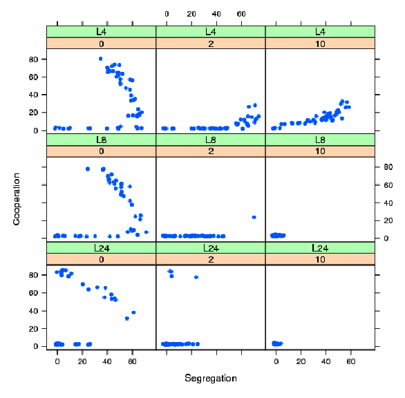
- 3.20
-
For error size 0, segregation and cooperation remain high both for L4, L8 and L24 although some runs end up near the full defection equilibrium with almost no segregation. Consistent with the preceding results, L4 and L8 have mostly segregated equilibria with some equilibria with small cooperation rates. For these equilibria, only small clusters of cooperators resist to defection. L24 has three types of equilibria: two non segregated, where equilibria are consistent with the global equilibria and some segregated equilibria.
Introducing noise changes the results: first for L4 and L8, the cooperation level becomes very small and segregation may remain high. Only a few small clusters of cooperation resist but overall cooperation is almost absent in the long run. For L8 and L24 and positive noise (2 or 10) almost all equilibria show low rates of cooperation (fig. 10). For L24 and positive noise, segregation is low in most of the cases and quasi absent for an error of 10. This shows that increasing sample size and error noise up to reasonable limits will lead to full defection in the triangular case. However, cooperation may be high and highly segregated for a long period of time before dropping to full defection: this is depicted by an example in figure 11.Figure 11: One simulation for the triangular distribution C=0.35, n=5, error size 2, T= 40000, L8. Cooperation level (left) and segregation level (right). 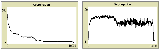
- 3.21
-
Note that in figure 11, before cooperation collapses, segregation is high which implies that cooperators may be preserved from defectors during these periods. Especially since cooperators earn more than defectors in small local interactions, other types of rationality, such as imitation of more successful individuals, could preserve cooperation.
Overall one concludes here that the distribution of emotions, and especially the level of the bifurcation point, is a central part for the emergence of segregated cooperation as shown in the next paragraph.
Varying the cost of cooperation
- 3.22
-
To further highlight the importance of the distribution of emotions on the final result, we vary the cost of cooperation and analyze, for each distribution, three cases summarized in table 2.
Table 2: Equilibrium prediction Uniform Triangular Costs 0.05 0.15 0.2 0.2 0.35 0.38 High Eq. 95 82 72.5 95 82 72.5 Bifurcation 5 18 28 23 49 61
- 3.23
-
The costs of cooperation are set so that the high equilibrium is respectively equal to 95, 82 and 72.5 for each distribution, uniform and triangular. For the uniform distribution, it corresponds to the respective costs of
0.05, 0.15 and 0.2, the latter being the case studied previously . For the triangular distribution, the costs are 0.2, 0.35 (preceding case) and 0.38. Thus, we compare three cases for which the same high equilibrium levels are expected, although the triangular distribution is always less favorable to the high equilibrium as shown by bifurcation points. Other parameters are set to T = 15000, n = 5,
= 2 and population size 100. For each combination of an interaction structure (L4, L8, L24, L44), a cost and a distribution, we performed 25 runs.
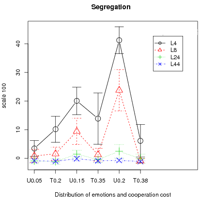
What should we expect? First of all since the bifurcation points are higher in the triangular case than their counterpart in the uniform case we should have, overall, higher cooperation rates for the uniform distribution. This is almost always the case. The only exception is for T0.2 (Triangular with C = 0.2) and U0.05 (Uniform with C = 0.05) for interaction structures L4 and L8 where cooperation rates are identical (left fig. 12).Figure 12: Average cooperation and segregation with 95% Confidence interval over 25 runs for different distributions of emotions and cooperation costs. 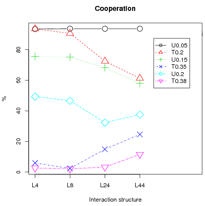
- 3.24
-
Second, one conjecture is that the stochastic stable equilibrium (Young 1998) is the full defection equilibrium whenever the bifurcation point is above 0.5 (T0.38). In that case, small local interactions should lead to full defection in the long run, implying smaller segregation levels than in the uniform counterpart. This is observed in left figure 12 where the cooperation rate is significantly different between U0.2 and T0.38 whatever the type of interactions. Especially, cooperation is almost null both for L4 and L8 in the T0.38 case implying that a bifurcation point below 0.5 is central for cooperation to persist (note that this is also true for T0.35). Therefore, segregation levels between U0.2 and T0.38 should also be different. This is observed in the right figure 12 where segregation for T0.38 is near zero for almost all interaction structures except L4, but for the latter, far lower than the U0.2 counterpart.
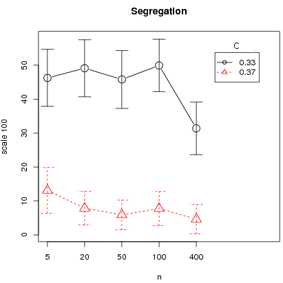
Finally except for the L4 interaction structure, the triangular distribution shows almost null segregation levels and segregation for the L4 and L8 cases is generally lower for the triangular distribution than in the uniform counterpart. This is consistent with the fact that, for L4 and L8 interactions, full defection is attained in almost all cases for the triangular, except T0.2. We run additional simulations for the L4 case in the case of the triangular distribution to test the critical importance of the bifurcation point for the results of segregation and cooperation. For this we take two costs: first, C = 0.33 for which the high equilibrium is at 84.9 and the bifurcation point at 44.3 ; second C = 0.37 for which the high equilibrium is at 76.9 and the bifurcation point at 55.7 . Other parameters are set to N = 400, memory = 30, T = 50000, error = 2 and
n = 5, 20, 50, 100, 400. For each (C, n) we run 50 simulations, controlling for initial conditions across different parameter configurations (C, n). That is the same 50 seeds are taken for each set (C, n) so that we have paired conditions between C = 0.33 and C = 0.37 for a given n. For initial conditions, 25 seeds are favorable to the full defection equilibrium that is with initial cooperation rates below 44.3 and 25 to the high equilibrium that is with initial cooperation rates above 55.7. Note that no initial condition has an initial cooperation rate between the two bifurcation points so that from the global equilibrium analysis, the same equilibrium are predicted for each paired condition. Figure 13 clearly shows that cooperation and segregation are higher for a bifurcation point below 50 percent. Moreover there seems to be a small effect of synchronous updating (n = 400) on segregation.
Figure 13: Average cooperation and segregation for L4 over 50 runs (with 95% confidence intervals) as a function of n for different costs c (triangular distribution). 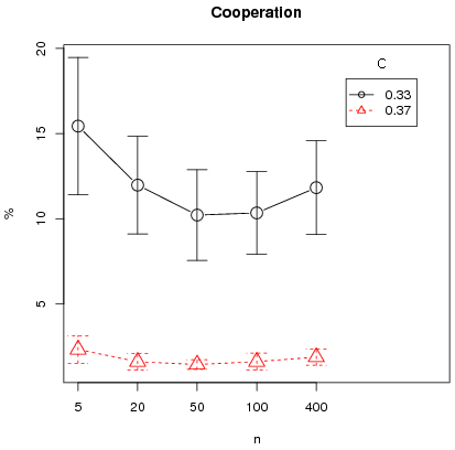
- 3.25
-
To conclude, segregation depends on the specific distribution of emotions.
When the high equilibrium has a larger basin of attraction as for the uniform distribution then segregated patterns emerge for small interaction structures. They disappear in the case of the triangular distribution with bifurcation above 50 (U0.2 in comparison to T0.38). For distributions with 2 stable fixed points, a bifurcation point below 50 is thus critical to large clusters of cooperation.
Conclusion
- 4.1
-
This paper introduced a modified PD game where players adhere more or less to the cooperative norm depending on the emotional intensity of deviating from it. Our modeling is, in some sense, a combination of methodological individualism, i.e. explaining cooperation by individual motives, and methodological holism by which cooperation is explained by the constraints the group exerts on individuals. The combination of real payoffs with emotions may lead to patterns explaining conditional cooperation and coexistence of cooperators and defectors in one shot games. Path dependency may lead to different types of equilibria. These two factors, i.e. the degree of adherence to a norm and history dependency, may be an explanation of the difference in cooperation among groups.
- 4.2
-
In addition, there is an ongoing debate in the social sciences as to whether institutions, here, the way individuals interact, or rationality is the most important factor in explaining emergent phenomena. The aim of this paper was to show that both aspects are important, i.e. the structure of interactions may be a factor explaining a large variance in outcomes across space. The result clearly shows that small localized interactions lead to segregated cooperation depending on the distribution of emotions (all results are summarized in table 4). Contrary to other papers, this result is not obtained by imitation. Indeed our individuals choose cooperation as a (stochastic) best response to real payoffs from a PD game. The only disturbing factor to segregated cooperation is in the case where the basin of attraction of the full defection equilibrium is larger than for the high equilibrium. In that case, full defection can be obtained in the long run, but the dynamics leading to defection may consist of segregated cooperation, suggesting that cooperation could be preserved by other types of rationality such as imitating the best strategy. Nevertheless the overall result that small interaction structure may lead to segregated cooperation, should be interpreted ''as a possibility condition" to the appearance of segregated cooperation.
Appendix A: Pseudo code
- A.1
-
Initialization: Place agents on the lattice and set up characteristics for all players (random initial strategy, random emotion).
- A.2
-
For each time step, the general procedure is:
- Some randomly chosen agents: Play the game
- Update global variables
- A new period starts
- To play the game: for n (
 N) players do
- count number of cooperators and defectors in a sample (local or random with a given size)
- compute payoffs (equation 4) for each strategy (cooperation and defection) given the strategy played in the preceding period by players in the sample and choose the best strategy with probability
(1 - ).
- Compute the fitness (real payoffs) from strategy
- Update the fitness list of each player (list of past and present fitness )
end
- To update all global variables
- update the list of strategies in the population
- compute the number of cooperators and defectors in the population
- compute average emotions of each sub-population of cooperators and defectors
- compute the average fitness of the population and in each sub-population of cooperators and defectors
- update a list stating whether players are happy or unhappy
- ask all players
[ ifelse ( my emotion > C / actual cooperate rate and (I am a defector) ]
- [set unhappy? 1 ]
- [set unhappy? 0 ]
- ask all players
[ ifelse ( my emotion > C / actual cooperate rate and (I am a defector) ]
- Count all unhappy players
- report the segregation level
end
- to report segregation levels
- given k (sample size) and the cooperation rate, compute the expected number of mixed pairs i.e. k × (percentage of cooperators ) × (1 - percentage of cooperators ) × population size
- ask each player: compute the number of players having a different strategy than myself in my sample of size k
- Sum over all players and divide by 2 to get the number of mixed pairs
- set segregation 100 × (1 - (mixed-pairs divided by expected-mixed-pairs))
Appendix B: Tables
-
Table 3: Average cooperation (over 30 periods) for different interaction structures and initial conditions in the case of a uniform distribution. 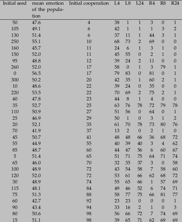
Table 4: Major results n Population Interaction structures Sample size T Distribution Cost Major result 5 2 100 Random and local 4,8,24 3000 U 0.2 Segregated cooperation for L4 and L8 5 0, 2, 10 100 Random and local 4,8,24 25000 U 0.2 Segregated cooperation for L4 and L8 5 2 100 Random and local 4,8,24 3000 , 25000 U 0.2 Segregated cooperation for L4 and L8 1, 5, 20, 100 2 100 Random and local 4,8,24 25000 U 0.2 Segregated cooperation for L4 and L8 5 2 100, 225, 400, 900, 1600 Local 4,8,24,44 10000 U 0.2 Segregated cooperation for L4 and L8, possible segregation for L24 and L44 for large population 5 0, 2, 10 400 Local 4,8,24 25000 T 0.35 Segregated cooperation vanishing in the long term but substantial in the mean term 5 2 100 Local 4,8,24 15000 U (cost = 0.05, 0.15, 0.2) and T (cost = 0.2, 0.35, 0.38) Higher bifurcation points lead to lower cooperation levels; the bifurcation level is critical to segregated cooperation. 5,20,50,100,400 2 400 Local 4 50000 T (cost = 0, 33 or 0.37) The bifurcation level is critical to segregated cooperation.
Notes
-
1
Support from the Agence Nationale de la Recherche ref. ANR-08-SYSC-008 is gratefully acknowledged.
The author would like to thank 3 anonymous reviewers for their valuable comments and suggestions. All errors remain my own. A preliminary version of this paper appeared under the name ''Segregation in social dilemmas''.
2 There is a large literature in psychology on the difference between shame and guilt but for the sake of our paper such difference will be ignored.
3 Simulations were done in Netlogo: http://ccl.northwestern.edu/netlogo/ (pseudo code in the appendix). The world is a torus meaning that agents in opposite sides are neighbours if within the distance of the sample size for local interactions.
4 T = 3000 is sufficient for the cooperation level to stabilize given the simulation parameters.
5 For the restricted parameter set, we eliminate from table 3 (appendix) seeds 35 and 110. For these seeds, the theoretical bifurcation point, given the mean emotion of the population, was at the initial cooperation level. It was not possible to decide whether we would expect a high or low equilibrium in these cases.
6 See Grauwin et al. (2012) for additional justifications and an application to segregation in Schelling's model.
7 Fitness of agent i in period t is simply the average fitness given
(t - 1). Total fitness of an agent equals to the sum of fitness over the last 30 periods, called memory of a run. To compare fitness with different parameters settings of memory, C or G, we normalized the total fitness of an agent to
(total fitness + C × memory)/(memory × (G + C)). It is this measure that is shown here. Note that each period only active players update their fitness. Additional simulations were done where all players updated their fitness or with fitness computed with actual play
(t) without notable changes in the results.
8 Note that random interaction structures do not lead to segregation so that the sensitivity analysis will be presented only for local interaction structures.
9 To allow for higher smoothing of noise, each variable represents now the average value over the last 50 periods of a run (instead of 30 in the preceding section).
10 Since the population size changes, we cannot control for identical initial conditions for different population sizes. T is chosen to make sure that for each parameter configuration, cooperation has stabilized.
11 Equivalent to Mann-Withney test but without assuming that samples have the same variance.
References
-
ALEXANDER, R. D. (1987).
The biology of moral systems.
New York: Aldine de Gruyter.
AXELROD, R. & HAMILTON, W. D. (1981). The evolution of cooperation. Science 211 (4489), 1390 -1396. [doi:10.1126/science.7466396]
BOLTON, G. E. & OCKENFELS, A. (2000). Erc: A theory of equity, reciprocity, and competition. American Economic Review 90(1), 166-193. http://ideas.repec.org/a/aea/aecrev/v90y2000i1p166-193.html. [doi:10.1257/aer.90.1.166]
BOWLES, S. & GINTIS, H. (2005). The Economy as an Evolving Complex System, III: Current Perspectives and Future Directions, chap. Prosocial Emotions. Oxford University Press.
BROCK, W. A. & DURLAUF, S. N. (2001). Interactions-based models. In: Handbook of Econometrics (HECKMAN, J. & LEAMER, E., eds.), vol. 5 of Handbook of Econometrics, chap. 54. Elsevier, pp. 3297-3380. http://ideas.repec.org/h/eee/ecochp/5-54.html. [doi:10.1016/s1573-4412(01)05007-3]
CAMERER, C. F. (2003). Behavioral game theory, experiments in strategic interaction. Princeton University Press.
CAMERER, C. F. & THALER, R. H. (1995). Ultimatums, dictators and manners. Journal of Economic Perspectives 9(2) 209-19. http://ideas.repec.org/a/aea/jecper/v9y1995i2p209-19.html. [doi:10.1257/jep.9.2.209]
CARRINGTON, W. J. & TROSKE, K. R. (1997). On measuring segregation in samples with small units. Journal of Business & Economic Statistics 15(4), 402-09. http://econpapers.repec.org/RePEc:bes:jnlbes:v:15:y:1997:i:4:p:402-09.
COHEN, M. D. & RIOLO, R. L. (2001). The role of social structure in the maintenance of cooperative regimes. Rationality and Society , 5-32. [doi:10.1177/104346301013001001]
DOEBELI, M. & HAUERT, C. (2005). Models of cooperation based on the prisoner's dilemma and the snowdrift game. Ecology Letters 8(7), 748-766. [doi:10.1111/j.1461-0248.2005.00773.x]
DUFWENBERG, M. & KIRCHSTEIGER, G. (2004). A theory of sequential reciprocity. Games and Economic Behavior 47(2), 268-298. http://ideas.repec.org/a/eee/gamebe/v47y2004i2p268-298.html. [doi:10.1016/j.geb.2003.06.003]
EGUİLUZ, V. M., ZIMMERMANN, M. G., CELA-CONDE, C. J. & SAN MIGUEL, M. (2005). Cooperation and the emergence of role differentiation in the dynamics of social networks. Am. J. Sociol. 110(4), 977. [doi:10.1086/428716]
EPSTEIN, J. M. (1997). Zones of cooperation in demographic prisoner's dilemma. Complexity 4, 36-48. [doi:10.1002/(SICI)1099-0526(199811/12)4:2<36::AID-CPLX9>3.0.CO;2-Z]
ESHEL, I., SAMUELSON, L. & SHAKED, A. (1998). Altruists, egoists, and hooligans in a local interaction model. American Economic Review 88(1), 157-79. http://ideas.repec.org/a/aea/aecrev/v88y1998i1p157-79.html.
FALK, A. & FISCHBACHER, U. (2006). A theory of reciprocity. Games and Economic Behavior 54(2), 293-315. http://ideas.repec.org/a/eee/gamebe/v54y2006i2p293-315.html. [doi:10.1016/j.geb.2005.03.001]
FEHR, E. & FISCHBACHER, U. (2004a). Social norms and human cooperation. Trends in Cognitive Sciences 8(4), 185-190. [doi:10.1016/j.tics.2004.02.007]
FEHR, E. & FISCHBACHER, U. (2004b). Third-party punishment and social norms. Evolution and Human Behavior 25(2), 63-87. [doi:10.1016/S1090-5138(04)00005-4]
FEHR, E., FISCHBACHER, U. & GäCHTER, S. (2002). Strong reciprocity, human cooperation, and the enforcement of social norms. Human Nature 13, 1, 1-25. [doi:10.1007/s12110-002-1012-7]
FEHR, E. & GäCHTER, S. (2000). Cooperation and punishment in public goods experiments. The American Economic Review 90(4), 980-994. [doi:10.1257/aer.90.4.980]
FEHR, E. & GäCHTER, S. (2002). Altruistic punishment in humans. Nature 415, 137-140. [doi:10.1038/415137a]
FEHR, E. & SCHMIDT, K. M. (1999). A theory of fairness, competition, and cooperation. The Quarterly Journal of Economics 114(3), 817-868. http://ideas.repec.org/a/tpr/qjecon/v114y1999i3p817-868.html. [doi:10.1162/003355399556151]
FISCHBACHER, U., GäCHTER, S. & FEHR, E. (2001). Are people conditionally cooperative? evidence from a public goods experiment. Economics Letters 71(3), 397-404. http://ideas.repec.org/a/eee/ecolet/v71y2001i3p397-404.html. [doi:10.1016/S0165-1765(01)00394-9]
FUDENBERG, D. & MASKIN, E. (1986). The folk theorem in repeated games with discounting or with incomplete information. Econometrica 54(3), 533-54. http://ideas.repec.org/a/ecm/emetrp/v54y1986i3p533-54.html. [doi:10.2307/1911307]
GLAESER, E. L., SACERDOTE, B. I. & SCHEINKMAN, J. A. (2003). The social multiplier. Journal of the European Economic Association 1(2-3), 345-353. http://ideas.repec.org/a/tpr/jeurec/v1y2003i2-3p345-353.html. [doi:10.1162/154247603322390982]
GLAESER, E. L. & SCHEINKMAN, J. (2000). Non-market interactions. Working Paper 8053, National Bureau of Economic Research. http://www.nber.org/papers/w8053. [doi:10.3386/w8053]
GORDON, M. B., PHAN, D., WALDECK, R. & NADAL, J.-P. (2005). Cooperation and free-riding with moral costs. In: International Conference on Cognitive Economics, August 5-8, Sofia, Bulgaria (PRESS, S. N., ed.).
GRAUWIN, S., GOFFETTE-NAGOT, F. & JENSEN, P. (2012). Dynamic models of residential segregation: an analytical solution . Journal of Public Economics 96, 1-2 124-141. [doi:10.1016/j.jpubeco.2011.08.011]
HAMILTON, W. (1964). The genetical evolution of social behaviour. i. Journal of Theoretical Biology 7(1), 1 - 16. http://www.sciencedirect.com/science/article/pii/0022519364900384. [doi:10.1016/0022-5193(64)90038-4]
HELBING, D., YU, W. & RAUHUT, H. (2011). Self-organization and emergence in social systems: Modeling the coevolution of social environments and cooperative behavior. The Journal of Mathematical Sociology 35(1-3), 177-208. [doi:10.1080/0022250X.2010.532258]
HENRICH, J., BOYD, R., BOWLES, S., CAMERER, C., FEHR, E., GINTIS, H. & MCELREATH, R. (2001). In search of homo economicus: Behavioral experiments in 15 small-scale societies. The American Economic Review 91(2), 73-78. [doi:10.1257/aer.91.2.73]
HENRICH, J., BOYD, R., BOWLES, S., CAMERER, C., FEHR, E., GINTIS, H., MCELREATH, R., ALVARD, M., BARR, A., ENSMINGER, J., HENRICH, N. S., HILL, K., WHITE, F. G., GURVEN, M., MARLOWE, F. W., PATTON, J. Q. & TRACER, D. (2005). in cross-cultural perspective: Behavioral experiments in 15 small-scale societies. Behavioral and Brain Sciences 28(06), 795-815. [doi:10.1017/S0140525X05000142]
KREPS, D. M., MILGROM, P., ROBERTS, J. & WILSON, R. (1982). Rational cooperation in the finitely repeated prisoners' dilemma. Journal of Economic Theory 27(2), 245-252. http://ideas.repec.org/a/eee/jetheo/v27y1982i2p245-252.html. [doi:10.1016/0022-0531(82)90029-1]
LEDYARD, J. O. (1995). Public Goods: A Survey of Experimental Research. In: A Handbook of Experimental Economics (ROTH, A. & KAGEL, J., eds.). Princeton, NJ: Princeton University Press, pp. 111-194.
LOEWENSTEIN, G. F., RICK, S. & COHEN, J. D. (2008). Neuroeconomics. Annual Review of Psychology 59, 647-670. [doi:10.1146/annurev.psych.59.103006.093710]
NOWAK, M. A., BONHOEFFER, S. & MAY, R. M. (1994). Spatial games and the maintenance of cooperation. Proceedings of the National Academy of Sciences of the United States of America 91(11), 4877-4881. http://www.pnas.org/content/91/11/4877.abstract. [doi:10.1073/pnas.91.11.4877]
NOWAK, M. A. & MAY, R. M. (1992). Evolutionary games and spatial chaos. Nature 359(6398), 826-829. [doi:10.1038/359826a0]
RABIN, M. (1993). Incorporating fairness into game theory and economics. American Economic Review 83(5), 1281-1302. http://ideas.repec.org/a/aea/aecrev/v83y1993i5p1281-1302.html.
SANFEY, A. G., RILLING, J. K., ARONSON, J. A., NYSTROM, L. E. & COHEN, J. D. (2003). The neural basis of economic decision-making in the ultimatum game. Science 300(5626), 1755-1758. http://www.sciencemag.org/content/300/5626/1755.abstract. [doi:10.1126/science.1082976]
TABIBNIA, G., SATPUTE, A. B. & LIEBERMAN, M. D. (2008). The sunny side of fairness. Psychological Science 19(4), 339-347. http://pss.sagepub.com/content/19/4/339.abstract. [doi:10.1111/j.1467-9280.2008.02091.x]
TRIVERS, R. (1971). The evolution of reciprocal altruism. Quarterly Review of Biology 46, 35-57. [doi:10.1086/406755]
WINTER, F., RAUHUT, H. & HELBING, D. (2012). How norms can generate conflict: An experiment on the failure of cooperative micro-motives on the macro-level. Social Forces 90, 3, 919-946. http://ideas.repec.org/p/jrp/jrpwrp/2009-087.html. [doi:10.1093/sf/sor028]
YOUNG, H. P. (1998). Individual strategy and social structure : an evolutionary theory of institutions / H. Peyton Young. Princeton University Press, Princeton, N.J. :. http://www.loc.gov/catdir/toc/prin031/97041419.html.
ZAK, P. J. (2005). The neuroeconomics of trust. SSRN eLibrary . [doi:10.2139/ssrn.764944]