Abstract

We introduce a model for agent specialization in small-scale human societies that incorporates planning based on social influence and economic state. Agents allocate their time among available tasks based on exchange, demand, competition from other agents, family needs, and previous experiences. Agents exchange and request goods using barter, balanced reciprocal exchange, and generalized reciprocal exchange. We use a weight-based reinforcement model for the allocation of resources among tasks. The Village Ecodynamics Project (VEP) area acts as our case study, and the work reported here extends previous versions of the VEP agent-based model ("Village"). This model simulates settlement and subsistence practices in Pueblo societies of the central Mesa Verde region between A.D. 600 and 1300. In the base model on which we build here, agents represent households seeking to minimize their caloric costs for obtaining enough calories, protein, fuel, and water from a landscape which is always changing due to both exogenous factors (climate) and human resource use. Compared to the baseline condition of no specialization, specialization in conjunction with barter increases population wealth, global population size, and degree of aggregation. Differences between scenarios for specialization in which agents use only a weight-based model for time allocation among tasks, and one in which they also consider social influence, are more subtle. The networks generated by barter in the latter scenario exhibit higher clustering coefficients, suggesting that social influence allows a few agents to assume particularly influential roles in the global exchange network.

Keywords:

Specialization, Agent-Based Modeling, Archaeology, Social Networks, Models of Social Influence, Barter

Introduction

1.1

Specialization is one way in which agents can increase their productivity (Murciano and Zamora 1997) by cooperating with other individuals (Spencer, Couzin and Franks 1998) to generate increasing returns to scale (population size of social group). The origins of specialization, especially craft specialization, have been linked with increasing sociopolitical complexity since at least the eighteenth century. Adam Smith (1776/1937) chose to begin his Inquiry into the Nature and Causes of the Wealth of Nations by suggesting that "the greatest improvement in the productive powers of labour, and the greater part of the skill, dexterity, and judgment with which it is any where directed, or applied, seem to have been the effects of the division of labour." He connected the origin of specialization with a human propensity to exchange, emphasizing that the interdependence produced by the joint action of specialization and exchange tends to increase overall productivity. Such increased production quite possibly initiated a positive feedback, since, for Childe (1936/1983), surplus production from an effective agriculture underwrote both technical and social divisions of labour, leading eventually in Mesopotamia to the emergence of elites who were able to support full-time craft specialists. Although specialization and production for exchange are often linked to the rise of the state, it is clear that they exist in smaller-scale societies alongside subsistence production (Patterson 2005).

1.2

In this article we develop an agent-based simulation of specialization in resource production, and a system of barter allowing exchange of specialized products, in Pueblo societies existing between AD 600 and 1300 in southwestern Colorado with the ultimate goal of examining their effects in these middle-range Neolithic societies. Since barter can mean rather different things, we specify that by barter we mean "moneyless market exchange" and not the sorts of reciprocal transactions that appear to be universally important in small-scale, non-market societies (Dalton 1982). Our goal here is to present the computational machinery making specialization and barter possible within our existing agent-based model. We are therefore less concerned with the realism of some of the assumptions below, including the amount of storage we allow, and the goods in which agents specialize. For example, specialization in production of ceramics is probably more likely in these societies (Harry 2005) than is specialization in making water available to other households; nor do we really believe that households in these societies were able to store the large quantities of goods we allow below. However, using these sometimes unrealistic assumptions, we hope to, as Epstein (2008: 3-4) says, "illuminate core dynamics" of the systems of barter and exchange and capture "behaviors of overarching interest" within the American Southwest.

1.3

Here we define specialization as the agents' choice to produce quantities of some goods in excess of a level needed for subsistence, while simultaneously underproducing other goods. When agents specialize, if they don't produce all their subsistence requirements, they must acquire these through exchange with other agents (Evans 1978). Specialization as we model it can occur along a spectrum. Agents can be fully specialized, performing one task (here, producing one good) to the exclusion of all others, or they can be partially specialized, performing all tasks to varying degrees. In our system, our agents are expected to be partially specialized, but it is also possible for some agents to become fully specialized.

1.4

As Smith realized, so long as exchange is relatively frictionless, specialization increases the productivity in a market system (Murciano and Zamora 1997). Productive individuals increase the supply for goods in which they specialize, and they specialize in producing goods in which they have a comparative advantage; at the same time they increase demand for other goods that they need, thereby providing indirect network effects (Young 1928). The level of specialization and output are dependent on several factors, including competition, the characteristics of the exchange networks, and initial conditions (Lavezzi 2003). Cockburn, Kobti and Kohler (2010) created an economic agent specialization model that added features not found in the simpler model produced by Lavezzi (2003), including consumption, production limits, changing populations, and changing trading relationships. The agents in that model were also sensitive to varying supplies of resources. If many agents are already outputting the same resource, the supply for that resource is likely to surpass the demand, thus discouraging additional production of that resource.

1.5

It has been shown that the level of specialization in complex systems, including human societies (Bonner 1993), is affected by the size of the system (Bonner 2004). Research in insect societies by Jeanson, Fewell, Gorelick, and Bertram (2007) indicates that when demand is low and there are many tasks, increased division of labour is an emergent property, suggesting that the level of specialization within insect societies is positively related to the size of colonies. The behaviour of cognitive agents can be modeled using motivation networks (Krink, Mayoh and Michalewicz 1999) in which agents choose between moving, eating and breeding based on conditions within the environment. Our agents are not this sophisticated, and only use specialization to determine what jobs to perform and how to divide their time among those tasks.

1.6

Cockburn and Kobti (2009b) and Cockburn et al. (2010) claim that introducing social influence into a system would increase the level of specialization. Building on these assertions, here we create a model that incorporates both economic state and social influence. Agents are influenced by competition from other agents in their topographically based social network. It is expected that there should be more task specialization in this socially influenced system than in the models without social influence. We also expect that the level of wealth will increase in the population (Murciano and Zamora 1997). Further, specialization and social influence may have effects on populations of agents, and as social influence interacts with exchange networks, we may expect specialization to change the structure of global populations. To assess the presence and size of these effects we compare systems in which (1) agents only try to procure enough resources to meet their needs; (2) where they plan based upon the economic state of their family, possibly producing more of some resources for which they have extractive advantage due to their location; and finally, (3) where they plan based upon their economic state while also considering competition from agents within their social network.

1.7

There are several approaches to modeling socially influenced specialization, including social inhibition, whereby agents discourage others from competing (Beshers and Fewell 2001). Temporal polyethism is another, where agents' specialization is related to their age (Ravary et al. 2007). Agents might also learn from experience (Murciano and Zamora 1997; Spencer et al. 1998; Theraulaz, Bonabeau and Deneubourg 1998), for example by randomly selecting a specialization at the outset, and if successful, selecting that action in the next round with higher probability.

1.8

For reinforcement-based systems to succeed in dynamic environments, agents must be able to overcome previously learned behaviour, especially when failure to do so results in death (Beaudreau 2003). Agents must be willing to engage in behaviour that previously had poor results and also must be able to respond to emergency situations, where change may be dramatic yet necessary. Moreover, the level of social influence within a society also affects the level of specialization. The more agents are affected by the actions of their neighbours, the more specialized the society becomes (see, for example, Cockburn and Kobti 2009a; 2009b).

Centralized Multi-agent systems

1.9

In Multi-Agent Systems (MAS), the study of specialization is often motivated by an interest in how specialization can increase the efficiency of the system in reaching its goals. A Markov-chain model to describe the evolutionary dynamics of the emergence of specialization in MAS is presented in Chai, Chen, Han, Di and Fan (2007). In that environment, agents search for and exploit resources with incomplete information and a goal of maximizing the efficiency of the entire system. The MAS uses a centralized model for determining task specialization, with task allocations emerging as a result of long-term system evolution. Thus, agents' specialization is determined by the overall needs of the system and not by individual considerations alone. As a result, an agent can sometimes be caused to specialize in tasks that are dangerous to its personal interests without sufficient reward (i.e., the job of cleaning up a toxic spill). Agent specialization in these systems will result in higher system productivity than in non-specialized systems (Chai et al. 2007).

1.10

Using a centralized specialization system also addresses another problem: agents generally do not possess complete information, thus any specialization decisions they make are likely to be suboptimal. Centralized MAS are better able to handle specialization in complex and changing environments (Chai et al. 2007), partly because they suppress complications arising from the self-adaptive striving of individual agents. Centralized systems also benefit from the fact that resources discovered by individuals can be more quickly exploited due to the global knowledge in the system and centralized direction.

1.11

Centralized MAS, however, put the burden on "the system" to be fully aware of all relevant factors in the decision-making process for all agents. There is no competition between agents in these systems. Such systems beg the question as to how societies of cooperating agents can emerge from societies of autonomous agents, since they assume that any conflict-of-interest problems in which cognitive agents might be tempted to override centralized decisions have been successfully solved. Finally, centralized direction is simply unrealistic for the case of the societies we model here, in which decision-making must have been more consensual and bottom-up than centralized (Van Vugt & Ahuja 2011).

Case Study: Village Ecodynamics Project

2.1

The Village Ecodynamics Project (VEP) is a multi-disciplinary, multi-institution project (Kohler et al. 2007). It has involved individuals from Washington State University, Crow Canyon Archaeological Center, Wayne State University, University of Windsor, Santa Fe Institute, Colorado School of Mines, University of Notre Dame, and BBL, Inc. Researchers include computer scientists, archaeologists, ecologists, anthropologists, geologists and economists. The VEP began by describing and modeling 1800 km² of the central Mesa Verde region of Southwest Colorado, occupied between A.D. 600 and 1300 by farmers ancestral to contemporary Pueblo peoples, which is the setting for this model. Thousands of habitation sites are known from this area, which we can assign to one or more of 14 periods based either on excavation or, in most cases, the ceramics on their surfaces (Varien, Ortman, Kohler, Glowacki and Johnson 2007). The entire northern Southwest was depopulated towards the end of the thirteenth century and one of the primary goals of the VEP research is to understand the reasons that led to this depopulation (Kohler, Varien, Wright and Kuckelman 2008). Another goal is to understand why, during certain times in prehistory, most people lived in large and relatively compact villages, while at other times, they dispersed into smaller hamlets (Crabtree 2012).

2.2

The original simulation was designed by Tim Kohler and colleagues at Washington State University and the Santa Fe Institute (Kohler, Kresl, van West, Carr and Wilshusen 2000). The simulation creates agent households that live, work, and reproduce in a landscape modeled on that of southwestern Colorado. Much of the dynamism of the simulation is provided by annual and spatially specific estimates of potential maize production on this landscape, originally developed by Van West (1994) and later refined by Kohler (e.g., 2012). Agent actions on this landscape are designed to be as realistic as possible, drawing on the considerable amount known about this place and time (Lipe, Varien and Wilshusen 1999). Agents are responsible for gathering their resources, while feeding their families and exchanging with other agents. Agents must farm maize, hunt for protein (cottontail rabbit, jackrabbit, and mule deer), obtain water from rivers and springs, and gather firewood from forests. Agents get all their energy, as measured in calories, from maize. When protein is required, it costs calories to procure. Agent households must provide their families with enough calories to perform these tasks, as well as provide for their basic metabolic needs. In the case that agents cannot obtain all the resources they need on their own, they are allowed to exchange with other agents. Families and family members are tracked in the model, and we allow different kinds of exchange relationships between kin, and among non-kin, drawing on models appropriate for small-scale societies (Sahlins 1972).

2.3

If an agent is not performing well at its present location, it will move to a more suitable location in the study area. Unfortunately for the agents, they are not allowed to exit the study area. When considering locations to move to, agents evaluate the resource productivity of prospective areas. This includes evaluating for farming productivity, water and fuelwood accessibility, and hunting opportunities. The model aims to represent soil productivity, rainfall, animal density, forest density, and other features of the region with a fair degree of realism. Even the vegetation that feeds the animals in the simulation is affected by climatic variability.

2.4

VEP researchers have identified two population cycles in the archaeological record (Varien et al. 2007). In the earlier, smaller cycle there is relatively little evidence for specialization, whereas in the later, more populous cycle there is evidence for specialization in at least the domain of political leadership, and probably also in provision of religious services and in aspects of ceramic production (Bernardini 2000). Ortman (2003) provides evidence that households relocating to the largest site in the VEP area, Yellow Jacket Pueblo, towards the end of its occupation specialized in ceramic production. This is possibly because, as late arrivals, the newcomers did not have access to high-quality farmland and needed to engage in craft activity to integrate with the economy. The framework we create here allows the emergence of resource-acquisition specialists within the simulation. Ceramic production specifically is not modeled but could later be added to the simulation.

2.5

Kohler and Varien (2012) present a great deal of additional information about the local archaeological record, the structure of the simulation, and our conclusions derived from comparing the two. The version of the simulation reported in that volume—on which this paper builds—is available at http://www.openabm.org/model/2518. Also notable in the present context are the investigations by Kobti et al. on the role of exchange in aggregation and depopulation, using cultural algorithms (Kobti, Reynolds and Kohler 2004; Reynolds, Kobti and Kohler 2004; Kobti and Reynolds 2005).

Approach

3.1

A more formalized description of our approach is presented in the appendix. Agents are allowed to divide their time among all four tasks existing within our simulation (farming, hunting, gathering wood and collecting water). The percentage of their time spent on each of these tasks is dependent upon their needs for the results of that task, as well as their perceived ability to obtain those resources more cheaply from close neighbours. If an agent has 30 kg less maize than it needs, it will seek to increase its maize production for the following year by 30 kg, by adjusting the percentage of its time that should permit that goal to be achieved. The agent will try to do the opposite if it is over its threshold for a resource. It will often happen that the agent will change multiple allocations, resulting in a total outlay not equal to 100%. At this point, the agent will normalize these allocations, such that it will spend 100% of its work hours on these tasks.

3.2

When agents have excess stores of a resource, they will let their neighbours know. Those neighbours that have higher production costs for these resources will predict that this agent will be able to help them meet any shortfall for this resource in the upcoming year. They will be willing to reduce their own production accordingly. The net result of these factors is that agents will dynamically adjust their allocations based on personal experience, as well as cooperation and competition from others.

Simulated environment

4.1

The VEP environment consists of four resources: water, wood, maize and meat. All but wood are needed for survival. While an agent dies immediately if it does not have enough maize or if it has been short of meat protein for three consecutive years, agents are allowed to survive continual shortages of wood (however, the agents don't factor this into their planning). While agents are bound by these resource requirements, they don't have any understanding of the consequences of resource shortfalls. This means that an agent does not prioritize water or maize over wood or protein, even though neglecting the former increases the chances of death.

4.2

Each resource is associated with a task that produces that resource. A farmer produces maize, a hunter acquires protein, a woodsman gathers wood, and a water carrier retrieves water. Each task also has constraints and requirements for the performance of that task. Farmers require land to plant their maize. There are a limited number of productive plots on the landscape and plots vary in productivity, both within a year (spatially) and from year to year. Hunting requires the presence of animals within the permissible hunting range of 4 km. Gathering wood requires the presence of deadwood or trees, and carrying water requires that there are water sources that the agent can travel to. For wood and water, agents are not bound by the distance to these resources; they can travel as far as necessary to obtain them. However all tasks require energy to perform, and thus require the agent to have sufficient calories to perform the task. The amount of energy required for these tasks was incorporated in the simulation before the development described here began, as explained in Kohler at al. (2007).

4.3

Agents must allocate their family's total calories available for the year among the given tasks. The number of calories required by each household is determined by the number of adults in the household, the number of children in the household, as well as how many hours per day each is required (or willing) to work. In the version of the simulation reported here, the number of hours willing to work was set to 6 hours/day for each individual in a family that is at or above working age (8 years old, in our simulation). Agents are able to spend any amount of their calories on any specific task. Agents also have a secondary goal, the accumulation (storage) of resources that increases their economic security for times when they cannot procure additional resources, such as during a famine or drought. All agents can only store a maximum of 10 years supply of any resource. A year's supply is the amount the household (agent) would need for subsistence estimated according to its current circumstances. It should be noted that while the maximum is set at 10, it is rarely the case that an agent possesses that much of a resource. Meat, for example, is rarely held in storage because of the scarcity of the resource and the high rate of decay. The maximum storage would theoretically allow a household specializing in hunting to store the meat from 10 deer while waiting to trade some for other resources. Any excess amount above the maximum allowed storage (10 years) will be donated to nearby relatives, or discarded if there are no relatives to accept them. While agents must sustain needs to survive, their focus is on maximizing their productivity given their abilities. All agents have the same skill level, so ability is delineated by the productivity of an agent at performing a task. Thus an agent having more productive plots would get a higher return on the energy expended on those plots, and thus can be claimed to be a "better" farmer than an agent with less productive plots. To prevent agents from dying before they have time to procure resources, all households are given an initial allocation of two year's supply of maize and meat, as these resources can only be gathered in autumn and summer respectively.

4.4

It is not feasible to initialize an agent's allocation among tasks randomly, since an allocation for farming that is too low would likely result in starvation, with similar unfortunate results for other resources. Additionally, the only way for a new agent to be introduced to the system is for a household to survive long enough to produce offspring. To address this problem, we have households calculate how much of each resource they need and allocate enough time to meet these needs. This only happens in the year in which a household is created. (Except at initialization, this is always due to a marriage.) We use the resulting allocation of time in that first year to seed our weights for the second year. If an agent spends 25% of its energy in the first year farming, then farming will have a 25% weight in our system during the second year. After this, agents rely on a performance and feedback function to update their weights for subsequent years. If agents may not be able to provide themselves with all the subsistence goods they need, they may trade for or request those resources through an exchange network.

4.5

The simulation reported here also modified the version reported in Kohler and Varien (2012) by allowing agents to pass on their wealth at death. If an agent household dies, the resources it has stored will be divided equally among its children who are within trading range, which is set at the same distance (8 km) permitted for balanced reciprocal exchanges (BRN; see below). If no children are within that range, this wealth is divided equally among neighbours, and finally, if no other agents are within range, the resources go to waste.

4.6

The general decision-making steps required of each agent are presented in Table 1.

Table 1: Decision-making process for each agent (household)
Step	Decision/action
1	If first year in current location, perform based on family needs and proceed to step 3. If not, proceed to step 2.
2	If second year in current location, use allocations from previous year to initialize weights. Proceed to step 3.
3	Perform tasks and expend energy.
4	Exchange resources if needed.
5	If still alive, update weights (defined in section 4.4).
6	If agent location not sustainable, move to new location.
7	Return to step 1.

Agent states

4.7

Agents have four states for each resource that affect their health and willingness to trade that resource. Calculations for each state depend on the size and makeup of each family. The calculations do not include usage of the resources for the purposes of working or performing other tasks. The states are based on how long the agents estimate the amount of the resource they possess will be able to meet their family's needs.

• TRADING - 2 years supply or more.
• SATISFIED - 6 months to 2 years supply.
• CRITICAL - less than 6 months supply (but more than 0).
• STARVING - When an agent doesn't have any of the resource, and needs to immediately obtain some via trading or begging.

Exchange

Barter

4.8

Barter—new to this version of the simulation—allows agents to trade one or more resources in exchange for another resource. Previous versions of the simulation allowed only generalized reciprocal exchange and balanced reciprocal exchange, and those only operated within the domains of meat and maize, as discussed below in §4.12 and §4.13. Moreover, the balanced reciprocal exchange system only allows time-delayed exchanges whereas barter simulates immediate exchanges. We have developed a simplified barter system in which agents trade goods based on a fair valuation. Prices are therefore not negotiated. To determine values for resources, we use the agent's cost of production. We accept that this does not result in the level of inequality that one would expect in a capitalist barter system where prices are negotiated. For instance, in a system with negotiation, we expect that if an agent (household) has the sole supply of a desired resource, it could inflate the price of that resource well beyond its cost of production. We did not include such a mechanism as it would unduly increase computational complexity. We use calories as a form of currency in this simulation. The interactions between the barter system, and the exchanges based on reciprocity, are outlined below in §4.18. We postpone for later investigation whether barter increases or decreases the degree of agent inequality (as measured for example by the Gini coefficient) relative to exchanges based only on generalized and balanced reciprocity.

Table 2: Variables used in barter
Abbreviation	Meaning
Ag	An agent
rAG	Some resource per agent
tAG	Agents in the set of potential trade partners
RWA	Set of resources an agent is willing to accept
REQag	Amount of given resource required by agent Ag

4.9

If for some resource rAG (Table 2 lists the abbreviations used to describe the barter algorithm) an agent is in a state of CRITICAL or STARVING, it tries to obtain enough of that resource to get back to a SATISFIED state. First it must identify agents that it can possibly trade with for the resource. It does so by the following process, which is repeated for each resource:

1. Ask each agent tAG (within trade range) if it is willing to trade the needed resource and what it is willing to accept in exchange.
2. Call the set of resources that tAG is willing to accept RWA(tAG)
3. If tAG has enough of the resource being requested by AG (tAG is in a TRADING state for that resource) and
4. If rAG has enough of one of the resources being demanded (in a SATISFIED state or better) by tAG, then add tAG to a list of trade partners, which we can call TList.
5. Sort TList in order of price for the resource being sought.

4.10

Since this process is repeated for each resource rAG sought, if the agent is in need of multiple resources, it will first seek to procure one, then after that (regardless of success), it will proceed to the next resource. After finding out which agents within its trade range are potential trade partners, AG must then ask these agents to trade in exchange for what it can offer them. That process is as follows:

4.11

For each agent tAG in TList:

1. Calculate how much of the required resource tAG is willing to offer. tAG is willing to offer any amount as long as it would not take it below its TRADING state.
2. Filter RWA(tAG), removing resources rAG not above the CRITICAL threshold for that resource. The resulting set can be called TRADE_SET.
3. Calculate how much of the required resource tAG is willing to offer (so that it doesn't fall below TRADING); we can call this set OFFER.
4. Limit OFFER to the amount rAG desired.
5. Calculate an amount for each resource in TRADE_SET that is equivalent in value to OFFER. rAG is not allowed to fall below SATISFIED for any or these resources.
6. If we can find a combination of such resources, then trade that combination of resources with tAG in exchange for the required resource.
7. If we cannot find such a combination, then calculate the maximum total value of resources that we are willing to trade with tAG.
   1. Calculate the amount of the required resource that tAG is willing to give for that value.
   2. Trade the selected amount of resources in exchange for the equivalent amount of the required resource that tAG is willing to give.
8. If rAG is now in a SATISFIED state, then stop, otherwise move to the next agent tAG in TList.

4.12

As stated, the value of a resource for an offering agent is determined by the cost to that agent of acquiring that resource. So if it costs an agent 1000 calories to acquire 10 kg of protein, then the value of that protein is 100 calories/kg. Agents do not question the value of resources as determined by other agents. Agents are however able to sort through those providing resources. Therefore an agent knows who in their neighbourhood can provide the resource most economically. This gives the requesting agent an advantage in the exchange relationship, as it can sort selling agents by lowest price, and selling agents will accept the cost to AG to produce the goods rAG being given in exchange.

Generalized Reciprocal Exchange

4.13

Even as we add barter, we maintain reciprocity-based exchanges in our system, since we can readily observe that even contemporary market societies retain kin and reputation-based reciprocal exchanges alongside market exchanges. We recognize two distinct systems of reciprocity, which we model separately. The first is based on kinship. An agent household knows the households of the parents of the husband and the wife as well as those of their siblings (again bilaterally). This leads to the introduction of the generalized reciprocal network (GRN), which operates over this bilateral kinship network (Kobti et al. 2004; Reynolds et al. 2004; Kobti and Reynolds 2005; Sahlins 1972). In GRN, agents are able to make requests for resources from members of their close kin. This provides a social safety net whereby related households band together to help each other survive. Agents are not expected to repay the resources that they obtain in the GRN, so if an agent obtains maize from a parent, they are not expected to repay that gift. This works out in the long run for agents because if that parent later were to ask the child for help, the child would reciprocate (Crabtree 2012; Sahlins 1972). Details on the internal logic of the GRN can be found in the papers listed above. In addition to requests, agents in the GRN in a TRADING state will donate some of their resources to a member of their family. All trading and donation in GRN in this instantiation of the model are limited to a geographical distance of 6 km, although this distance is changeable. Moreover, kin will not put themselves below the SATISFIED state to help, as this may put their own household at risk, and importantly, GRN is only implemented for maize and meat. The order in which the three types of exchange networks are activated is outlined below.

Balanced Reciprocal Exchange

4.14

The balanced reciprocal exchange network (BRN) is a reputation-based borrowing/loaning network that enables agents to exchange maize or meat with neighbours who are not kin in the expectation that they will be repaid the same amount of the same resource at a later date. This is probabilistic, so agents will not automatically loan to someone requesting, even if that household has a good or neutral reputation (in this model, we allow a 75% chance of saying yes to these individuals). If an agent loans a resource to a neighbour (here defined as a household within BRN trading distance of 8 km, but like GRN this distance can be modified), it expects to receive that resource back when it asks for it. Agents will ask to be repaid once per year, at the end of the harvest, or immediately if the agent is in dire need (in a STARVING state; however, agents, as in the GRN, will not exchange if they are below a user-specified state for risk of death by starvation). If the neighbour repays when asked, then its reputation remains intact. If the neighbour is unable to repay the loan, this will damage its reputation. Reputations are only dyadic (between two agents), so an agent could have a negative reputation with one agent while being held in high esteem by another (Crabtree 2012).

4.15

Agents are able to improve their reputations by loaning resources. If a neighbour loans an agent a resource, its reputation with that agent goes up. This means that later if this neighbour is in need of another resource that its partner in a previous exchange can provide, this partner is more likely do so. Resource transaction in the BRN is like-for-like. This means that if an agent is loaned some maize, the debt is repaid in maize. As for GRN, BRN is only implemented for maize and meat.

4.16

Neighbours (those agents in a BRN) are much less generous than kin (agents in a GRN). An agent has to be in a TRADING state before it will consider making a BRN exchange. Then the reputation of the asking agent is considered. The asking agent needs a positive or neutral reputation before the neighbour will proceed. If these two requirements are met, the agent will consider whether it is in a "loaning mood" (as determined by the probability noted above). An agent will not allow itself to fall below a TRADING state in loaning a resource to a neighbour.

4.17

BRN promotes a strong "community" bond among agents, though these bonds are only expressed dyadically. While agents do not account for this (in either their movement algorithm, or by seeking to enhance their reputations as a goal) larger communities with more positive linkages provide more opportunities for trade and assistance. Of course this is balanced by competition for resources; if local populations become too large, resources may become limiting. This can result in agents having to leave their community to find a more productive location, even at the cost of losing their current trade partners. Note that while we use the word community, this is not a physical construct within the simulation. Here we regard a community simply as a network of agents within a certain radius, tied together by their exchange practices.

Sequence of exchanges in the model

4.18

Agents first seek to obtain the needed amount of a resource via the barter network. If the agent still has not obtained enough of the resource it needs from its trading partners and it's in a STARVING state, it attempts to use one of the reciprocity networks. First the agent uses the GRN to ask up to 4 kin (this number is a changeable parameter in the simulation) to give it the amount it's short. If it cannot obtain enough via this method, it then tries to borrow using the BRN. If after all this, rAG is still deficient, then AG dies if the resource is mandatory (water, maize) or suffers malnutrition (protein), which may also lead to death after 3 years. Since balanced and generalized reciprocity exchanges only pertain to protein and maize, agents can obtain water and wood only via barter or by direct procurement.

Social Influence

4.19

Agents' behaviours may be influenced by the behaviours of those around them (Waibel, Floreano, Magnenat and Keller 2006). Given a choice between multiple specializations, we factor in what an agent's neighbours are doing and allow that to influence the agent's decision. An agent N is defined as a neighbour of an agent Ag if N and Ag are directly connected within a social network (for our simulation this network is limited to the trade radius of BRN). It has been shown that social influence often can increase the level of agent specialization when compared to systems with no social influence (Cockburn and Kobti 2009a). Cockburn and Kobti (2011) showed that a weight-allocated social pressure system would be capable of stimulating the emergence of a high level of specialization within a population. We base our current model on that method.

4.20

For each agent Ag, there should exist a composite function Soc(t) for each task t in EC. Soc(t) would be a function representing the social influence towards performing task t. An example of such a function would be peer pressure towards performing a task. In an economic network, the social influence may be a reflection of the demand for a product. In such a situation, it is also possible to create the social influence function such that there also exists negative influence. An example of this would be negative influence in the case of a potential sale that's lost because a competitor can provide a better product. The handling of the result of Soc(t) is dependent upon the agent and the domain. Given the same example of an agent selling a product and the same demand-influence function, an agent may reduce production or reduce the price of its product.

4.21

For our case, we first designate r(t) as the resource produced by task t. Each agent requesting a resource r(t) exerts production pressure on its possible trade partners in the following manner:

1. Locate all agents within trade range, placing them in a list we call POSS
2. Determine an influence rate IR=1/the size of POSS
3. Let rAmount = amount of resource r(t) that Ag is seeking to procure
4. For agent tAG in POSS
   1. exert upward production pressure on tAG for task t in the amount of rAmount × IR (for tAG: Soc(t) = Soc(t) + rAmount × IR)
   2. Let tAmount = amount of resource r(t) that tAG has available, OR rAmount, whichever is lower
   3. exert downward production pressure on tAG for task t in the amount of 2 × tAmount × IR (for tAG: Soc(t) = Soc(t) + amountTraded × IR)
   4. If tAG and Ag completed a trade for r(t)
      1. Then amountTraded = the amount of r(t) traded between Ag and tAG
      2. Exert upward production pressure on tAG for task t in the amount of amountTraded × IR (for tAG: Soc(t) = Soc(t) + amountTraded × IR)

(Interpretations of quantities: 4a indicates to each agent that may provide the resource that this agent has a demand for the resource; 4c: This pressure accords with an agent's expectation of completing a trade for the amount possible (tAmount). If the agent completes the trade, the pressure will be reversed based on the amount of resource traded. If the agent is unable to sell, then this is either because there exists another agent that was a better trade partner for the requesting agent, or the requesting agent did not have the resources that the selling agent was demanding in exchange for the resource. 4dii: This rewards the expectation of sale. The net effect is that if an agent is asked for a resource and is able to provide it, then that means their current level of production is sufficient to meet demand.)

4.22

A selling agent Ag, having excess resources available at the end of a production period (in a TRADING state) also exerts pressure on its competitors in the following manner:

1. Locate all agents within trade range, placing them in a list we call POSS
2. Determine an influence rate IR = 1 / the size of POSS
3. Let rAmount = amount of resource r(t) that Ag has that it is still willing to trade
4. For agent tAG in POSS
   1. If production cost of r(t) is higher for tAG than for Ag
      1. Exert downward production pressure on tAG in the amount of rAmount × IR (stated differently: Soc(t) = Soc(t) - rAmount × IR for tAG)

4.23

Therefore an agent will attempt to indicate to competitors with higher production costs that it is a better source of the resource and that it would be more capable of providing that resource to them. This deals with agents who are within range of each other, but are both self-sufficient with regards to a resource. Exerting competitive pressure encourages the less efficient agents to lower their production and rely on the more efficient ones for the resource.

4.24

An agent that is pressured socially does not have to change its behaviour. Sometimes, if an agent is already in a TRADING state for a resource, they will ignore pressure to increase production. The reason behind this behaviour is that the agent determines that it already had surplus, but no one was able to exchange for it (possibly because no agent has anything to offer that the agent is willing to accept). In that case, increasing production will not lead to an increase in trade. Agents also will not decrease production if they are below a SATISFIED state. This occurs if the agent determines it could not procure more of the resource because it did not have anything to trade to the selling agents. Therefore reducing their production will not result in them obtaining more needed goods and would therefore be antithetical to their survival.

Update function

4.25

We use a uniform update function for each task in our weight system. This update function is applied at the end of each year, and determines how the agent will allocate time for the upcoming year. Given task t that provides resource r and x amount of resource r:

1. If the agent is in a TRADING state, then assume y = x - the threshold for TRADING. The agent will then reduce the weight of task t proportionally so it should result in the agent producing y less of r than it produced this year. In other words, if the agent has 200 kg too much maize, then it will reduce the weight it applies to farming so that the agent expects to produce 200 kg less maize next year. To avoid an agent making too drastic a cut, based perhaps on an abnormal amount of a resource because of trading, we restrict the amount an agent is allowed to reduce a weight to 50% of the current value.
2. If an agent is in a CRITICAL or STARVING state, then the agent will attempt to increase the weight for the task t so that it expects to produce enough additional resources in the following year to get it to a SATISFIED state. Again, to avoid overcompensating, we restrict the maximum increase to 300%.
3. Apply any social pressure as determined previously.

Results

5.1

To evaluate the impacts of these additions to the base simulation, we ran the simulation three times, once with agents allocating effort based only on family needs (Scenario 1), which is similar to the original simulation but with additions such as the barter network and resource inheritance. We do not expect this scenario to result in much specialization. We then ran the simulation with agents allocating effort based only on their current economic state (Scenario 2). In that case, agents set their weights for tasks based on the amount of a resource they have remaining. If they have more than they need based on their reserve threshold (TRADING state), then they reduce production. They increase production if they are below this level. The calculation for this update was explained previously. Finally we ran the simulation with both economic state considerations and social influence enabled (Scenario 3). With the addition of social influence, agents will reduce their production of a resource if they are in a TRADING state and there is an agent available that can provide the resource more cheaply than the agent's cost of production.

5.2

We compare the different methods using several measures. One such measure is the level of task specialization (as explained below), which is applicable only to the second and third scenarios. We also compare the proportion of the population in each of three "settlement types" differentiated by the number of households cohabiting specific cells in the model. We also note the change in the volume of exchange when agents allocate based only on needs, and when they attempt to specialize. Additionally, we measure the accumulated wealth (measured as defined below) of the population under these three scenarios.

5.3

Finally, we compare the structure of the exchange networks that form in Scenario 2, and in Scenario 3, using an approach designed to reveal the degree of compartmentalization in the networks. The exchange network provides another means of characterizing the overall structure of the system; for example, how does the degree of specialization affect the structure of these exchange networks? In network analysis one analyzes the frequency of nodes (the agents) and the frequency of edges (here, the exchanges between agents) (Newman 2010). By understanding how the connectance (the proportion of possible links between agents that are realized) of each agent changes, and variability in the number of edges, we can better understand phenomena of interest in the reference system such as the resilience of the network to perturbation or the efficiency of the network in distributing goods or information. We presume that different network structures have different outcomes for transmission of influence, innovations, and socially influenced behaviours in general. Below we contrast years of high and low population within and between scenarios.

5.4

To measure the degree of task specialization, we use a method developed in Gorelick, Bertram, Killeen and Fewell (2004) to calculate the level of task specialization within the system. We use the weight given to each task to calculate the level of task specialization at the end of each step in the simulation. The weights of all agents are then stored in an n-x-m matrix, where n is the number of agents and m is the number of tasks. Therefore each row in the matrix represents an agent's time allocation among all tasks. The matrix is then normalized such that the total of all values in the matrix is 1. The mutual information and Shannon entropy index (Shannon 1948) are then calculated for the distribution of agents across tasks. The Shannon entropy is then divided by the mutual information score, resulting in a value between 0 and 1. A value of 1 indicates that all agents spend all their time on one task (not of course in the same task), while a score of 0 means that there is no task specialization, as would be the case when each agent divides its time equally among tasks. See Gorelick et al. (2004) for a full explanation of this method.

Effects on Population Size and Degree of Specialization

5.5

As can be seen in Figure 1, and as expected, there is a marked increase in population size when specialization is added (Scenario 2 vs. 1). Somewhat surprising is that population levels are slightly lower when social influence is added to economic specialization, though populations converge late in the simulation (Scenario 3 vs. 2). Perhaps the addition of social influence can make agents too reliant on the success of others for their own success, somewhat analogous to Hegmon's demonstration that sharing too broadly can be detrimental to community survival (Hegmon 1989). Another potential explanation may be that since agents here do not consider social networks when moving, they may be able to move outside of their social network, populating an area where they have no exchange partners. This increases the likelihood that agents will not be able to exchange until they are able to rebuild an exchange network (Crabtree 2012).

5.6

We also found that the degree of production specialization increased significantly as we added social influence to the factors that agents consider (Figure 2, Scenario 3 vs. 2). This further confirms the findings of Cockburn and Kobti (2009a; 2009b). In all figures, AD 600 corresponds with the initial colonization of the VEP area by farmers. However, this area was in fact depopulated around AD 1280, a fact not replicated in these simulations. Instead, we see a spike in the levels of specialization around this time in our simulation.

5.7

There are factors to be noted in the performance of the underlying specialization mechanism that we were not able to fully explore here. Namely, the number of years of storage we allow each agent is very important. As we have no monetary currency (outside of caloric costs) and do not allow exchanges of goods for labour, stored resources are the only source of wealth and assets for exchange. Investigations not presented here show that the level of specialization increases as we increase the number of years of storage allowed. We can conclude that adding social influence to our reference system with economic specialization leads to a population that is not necessarily larger in size, but one that is more specialized.

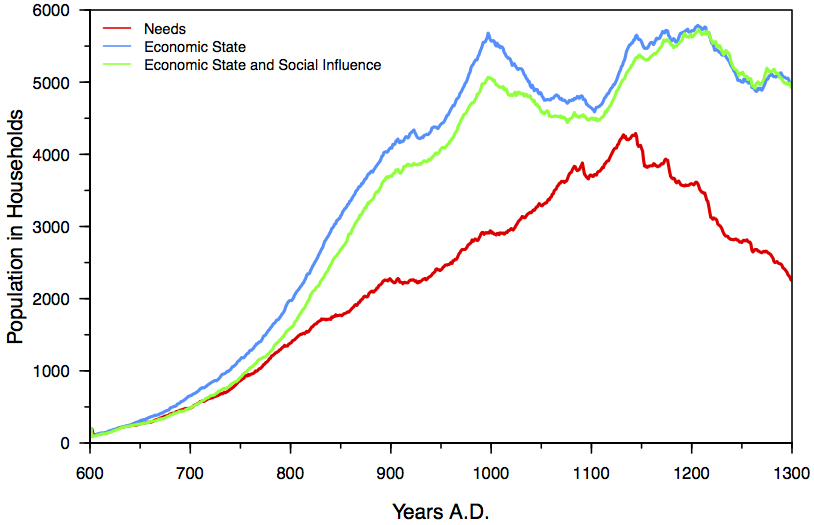
Figure 1. Population levels for each of the three scenarios; Scenario 1 needs only; Scenario 2 economic state; Scenario 3 based on both economic state and social influence. To note is how much higher populations are when they are not based on needs only.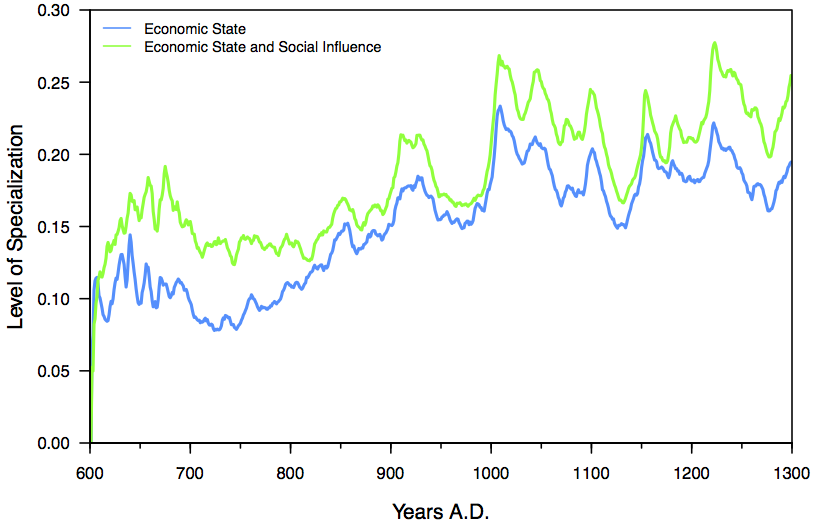

Figure 2. The degree of production specialization between Scenario 2 for economic state and Scenario 3 for economic state and social influence.

Effects on Degree of Aggregation

5.8

As noted, agents will move if they are not thriving at their current location. When choosing a destination, agents do not factor in the presence of potential exchange partners, or any exchange networks that may exist among those households, unlike in Crabtree (2012). Our results show that agents are more likely to cohabit the same cell when they specialize, as seen in Figure 3. Without specialization, agents primarily live in small hamlets of 1-2 households, and few in community centers (of 9 or more households). We found that with just economic state influencing planning (Scenario 2 vs. 1), agents are more likely to live in big hamlets (3-8 households), surpassing the proportion living in smaller hamlets after about AD 750 in the runs presented here. The proportion of agents living in community centers is also greater in either scenario 2 or 3 than in 1. This may suggest that agents move less as a result of specialization, or it may suggest that they are better able to tolerate the effects of scramble competition for resources when their resource needs are complementary rather than redundant. More generally these results suggest that an increase in specialization might often lead to increases in sizes of the largest sites, and in the degree of aggregation, in the archaeological record.

5.9

Interestingly, when comparing Scenario 3 vs. 2, we see that agents taking into account only economic state (Scenario 2) are more likely to live in community centers (> 8 households) for most of the simulation. Agents in Scenario 3 are more likely to live in big hamlets (of 3-8 households) than are the Scenario 2 agents. These differences are relatively slight, however, and might disappear if we were to repeat this exercise using multiple realizations of each of these economic scenarios using different random number seeds and different parameter settings for basic agent operation. The stronger signal is the clear difference between the greater aggregation expected under Scenarios 2 or 3 relative to Scenario 1.

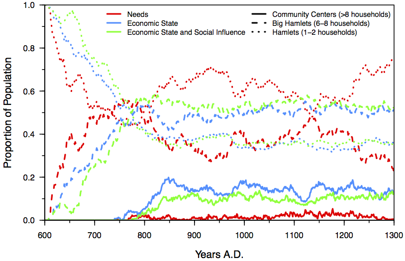
Figure 3. Proportion of households in each type of settlement, hamlets, big hamlets and community centers for Scenario 1 needs, Scenario 2 economic state and Scenario 3 economic state and social influence.

Effects on Volume of Exchange

5.10

Along with an increase in the proportion of households living in larger communities, we observed a significant increase in barter under either of the scenarios promoting specialization, compared to the condition where agents allocate efforts based on their private subsistence requirements (Scenario 1). This is due in part to workers working more hours on average, and thus trying to produce more than they need to meet their family's needs. The excess supply of resources results in more agents in shortage being able to find someone willing to meet that demand. We see in Figure 4 that there is very little trading in some resources such as wood in the "needs only" scenario (whereas much is requested, but almost none is exchanged). With agents just trying to produce enough for their own family, it's unlikely that they will overproduce, and so they accumulate no exchangeable surplus. Therefore there is no barter, despite the fact that there still is a high level of demand for wood. With the change in allocation strategy more of the demand for such resources can be met because there is more overproduction of resources. Although the level of demand is not fully met under specialization, the unmet demand is much less than in the "needs only" scenario.

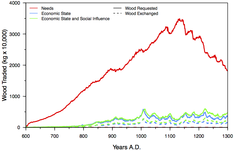
Figure 4. Volume of exchange of wood per scenario; solid line depicts requested wood, while dotted line requests exchanged wood. Note how in Scenario 1 the needs only scenario wood is requested frequently but seldom exchanged.

Effects on Volume of Storage

5.11

Figure 5 reveals that when agents allocate their labour based only on needs (Scenario 1), we found that they store less than in the specialization scenarios (2 and 3), despite the fact that their storage restrictions are identical. This is as expected since agents procuring only what they need rarely overproduce. Overproduction in that case is due either to the inability of an agent to accurately estimate the needs of its family, or inability to procure exactly the amount required (for example it's not possible to only kill half a deer). On the other hand, when allocating labour based on economic and social factors, agents are much more productive. The resources they overproduce are maintained in the system (the society), resulting in higher average agent wealth. We can see that there is still a low storage amount for meat. This is due both to the high decay rate for this resource in storage, as well as the landscape-wide depression of the most important meat source, deer (both in our models, and in the world they reference). Average storage levels do not change noticeably when social influence is added to economic specialization, even though that addition results in a small increase of specialization, as we saw in section 5.1.

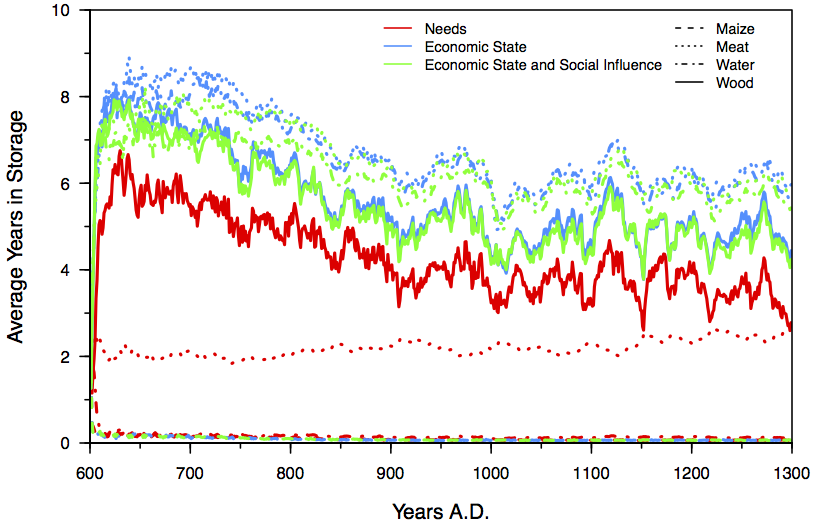
Figure 5. Storage based on each scenario. Note that in the needs based scenario, Scenario 1, agents store much less than in the other two scenarios.

Effects on Social Networks

5.12

As seen above, exchange increases when economic state and social influence are taken into account, as shown in Figure 4 for wood. Additionally, storage of most resources is greater when agents specialize than when they only take into account their needs, as seen in Figure 5. Finally, when agents specialize, populations increase (see Figure 4 for example). These three results lead us to expect that the social networks that form from bartering of each of these resources will be markedly different among the three scenarios: when agents take into account only their needs (Scenario 1) and when they specialize (Scenarios 2 and 3). Performing a network analysis on the dyadic exchanges between agents provides a means for comparing the structure of the system emerging from these interactions.

5.13

For this analysis we identified four points in time (as reported in Table 3) from Scenarios 2 and 3. Table 4 reports the number of exchanges through time in the barter network for Scenario 2. Table 5 reports the corresponding figures when allocation of effort is based on economic state and social influence (Scenario 3).

5.14

Not surprisingly, when the simulation begins exchange is high. When the agents are initially seeded, randomly, on the landscape, many are placed in areas with poor production. Consequently the agents try to make up for deficiencies of resources by bartering with one another. With respect to the number of edges per node, both Scenario 2 and 3 are rather similar, and decline slightly through time. However, except in the first year of the simulation, Scenario 3 always generates more exchanging agents—nodes—and more exchanges—edges—than does Scenario 2.

5.15

Another interesting contrast between the two scenarios lies is in the differing degree of the clustering coefficient that each network generates. The network's clustering coefficient is the measurement of the number of edges between the neighbours of a node n divided by the maximum number of edges that could exist between the neighbours of node n, as described in Assenov, Ramirez, Schelhorn, Lengauer and Albrecht (2008). The clustering coefficient of a node n is:

Cn=en/(kn(kn-1))

"where k_n is the number of neighbors n, and e_n is the number of connected pairs between all neighbors of n" (Assenov et al. 2008 Network Analyzer Supplemental Materials). The clustering coefficient of a node is always scaled between 0 and 1, which allows for comparability (Assenov et al. 2008; Doncheva et al. 2012). In this context, a higher clustering coefficient means that the entire system of exchanges exhibits more clustering into condensed components. A lower clustering coefficient means that the system of exchanges is more dispersed overall. Note that this is "aspatial" in that the clustering of exchanges is not necessarily related to the location of agents on the landscape. Here, we calculate the clustering coefficient as averaged across all of the nodes to give a clustering coefficient for the entire network. Clustering coefficients are calculated differently depending upon whether the network is directed or undirected. Networks of exchange are directed, since one household is providing resources for another, so analyses are based on directionality; even though exchange is reciprocal, each exchange itself is directional. For this analysis the clustering coefficient is computed for directed networks. These results are reported below in Figure 6.

5.16

Comparing Scenarios 2 and 3, we see in Figure 6 and Table 5 that the socially influenced network generally exhibits a higher clustering coefficient even as the overall connectivity of the agents is declining. This suggests that the socially influenced network (Scenario 3) is more reliant on a few nodes to supply the rest of the network. Bascompte (2010) characterizes the reliance on few nodes to supply the network as a "compartmentalization" or "the tendency of a complex network to become organized in 'compartments' characterized by a group of species interacting more strongly among themselves" (Bascompte 2010: 765).

5.17

Though Bascompte refers to biological networks, compartmentalization is similarly useful here. Instead of different species interacting, the compartments are formed of groups of agents who together can be conceptualized as communities. For example, in year 1100 of Scenario 3 (Figure 7c) the overall network has been divided into multiple groups; some of these groups are connected through just a few individuals. There are also outlying groups that are completely cut off from the flow of goods in the main network and other subnetworks. These networks appear to be more compartmentalized, as also indicated by the slightly higher clustering coefficient in Table 5, than the networks generated under Scenario 2.

5.18

If one wanted to disrupt the flow of the Scenario 3 networks there are certain nodes that would be instrumental to destroy. In Scenario 2 year 1100 (Figure 6c), on the other hand, there is a more equal distribution of node interactions; if one random node were to be removed, it would be less disruptive to the overall flow of the network since node-to-edge distribution is fairly equal. In Scenario 3 if one were to remove a random node there would be a high probability of removing a non-essential node. However, if, perchance, one of the "hub" nodes (the node with the most connections) were removed, its entire network would collapse. The hub nodes provide the bulk of the interactions, and once removed more compartmentalization would occur—portions of the network would no longer be connected to each other (see Reynolds, Kobti, Kohler and Yap 2005).

Table 3: Characteristics of population at years when networks are assessed
Year	Characteristic of population
600	Start of simulation
1000	Population peak
1100	Population trough
1200	Population peak
1300	Population trough

5.19

We have not yet investigated whether the "hub nodes" of Scenario 3 are also relatively wealthy, though it is likely that they have both large families, and more storage than average; we do know they are relatively "rich" in the number of connections they have. We also hypothesize that they are advantageously placed on the landscape both with respect to landscape productivity and with respect to their ability to act as intermediaries between two network segments because of their location. Clearly they are instrumental to the distribution of the goods.

5.20

Upon visual inspection of the figures we can see that exchanges look very similar in year 600 for both strategies (Figures 7a and 8a). For year 1100, in the network created by Scenario 2 agents there are few exchanges, and it appears that each exchanging agent is equally connected. However, in year 1100 under Scenario 3 we see that exchange is more frequent. Possibly the social influence that helps to create "hub" nodes also facilitate exchange among larger numbers of agents than is possible through economic state alone.

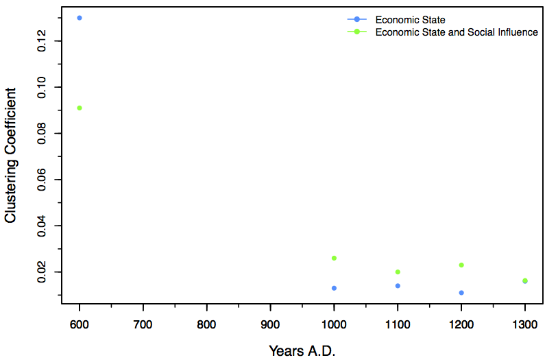
Figure 6. Network clustering coefficient for each of Scenario 2 economic state and Scenario 3 economic state plus social influence for year 600, 1000, 1100, 1200 and 1300. Coefficients are reported in Table 4 and Table 5.

Table 4: Connectivity when allocating only based on economic state (Scenario 2)
Year	Nodes	Edges	Network Clustering Coefficient	Number edges/node
600	181	478	0.130	2.64
1000	595	1592	0.013	2.68
1100	443	1194	0.014	2.70
1200	271	678	0.011	2.50
1300	317	749	0.016	2.36

Table 5: Connectivity when allocating based on economic state and social influence (Scenario 3)
Year	Nodes	Edges	Network Clustering Coefficient	Number edges/node
600	180	468	0.091	2.60
1000	625	1746	0.026	2.79
1100	495	1320	0.020	2.67
1200	455	1160	0.023	2.55
1300	470	1185	0.016	2.52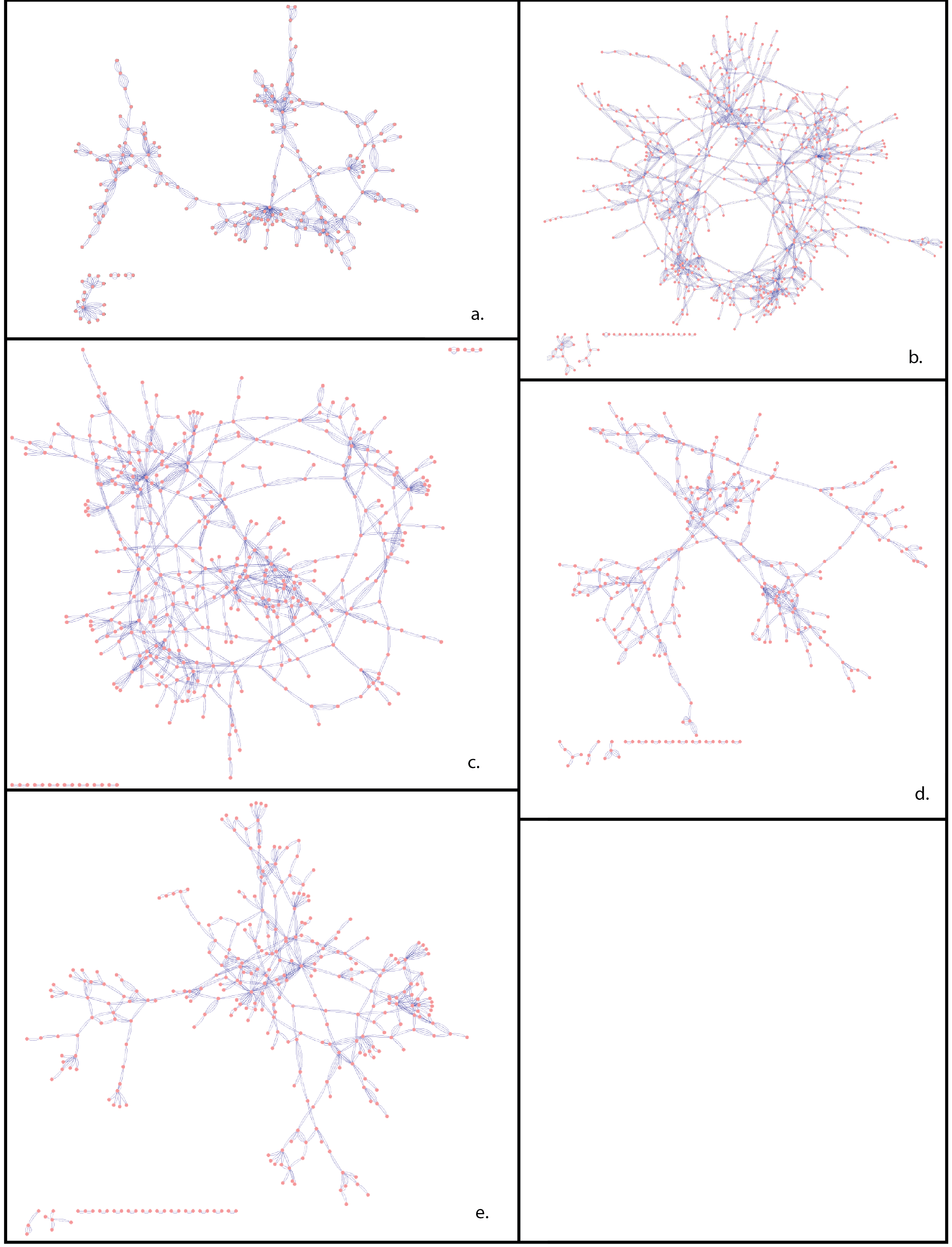

Figure 7. Example exchange networks, scenario 2. Pink dots represent households and blue lines represent exchanges. Multiple lines represent multiple exchanges for those households. a. year 600, b. year 1000, c. year 1100, d. year 1200, e. year 1300. Graphs are formed based on connectance, not on physical space. Nodes toward the edges are the least connected, while nodes toward the center are the most connected.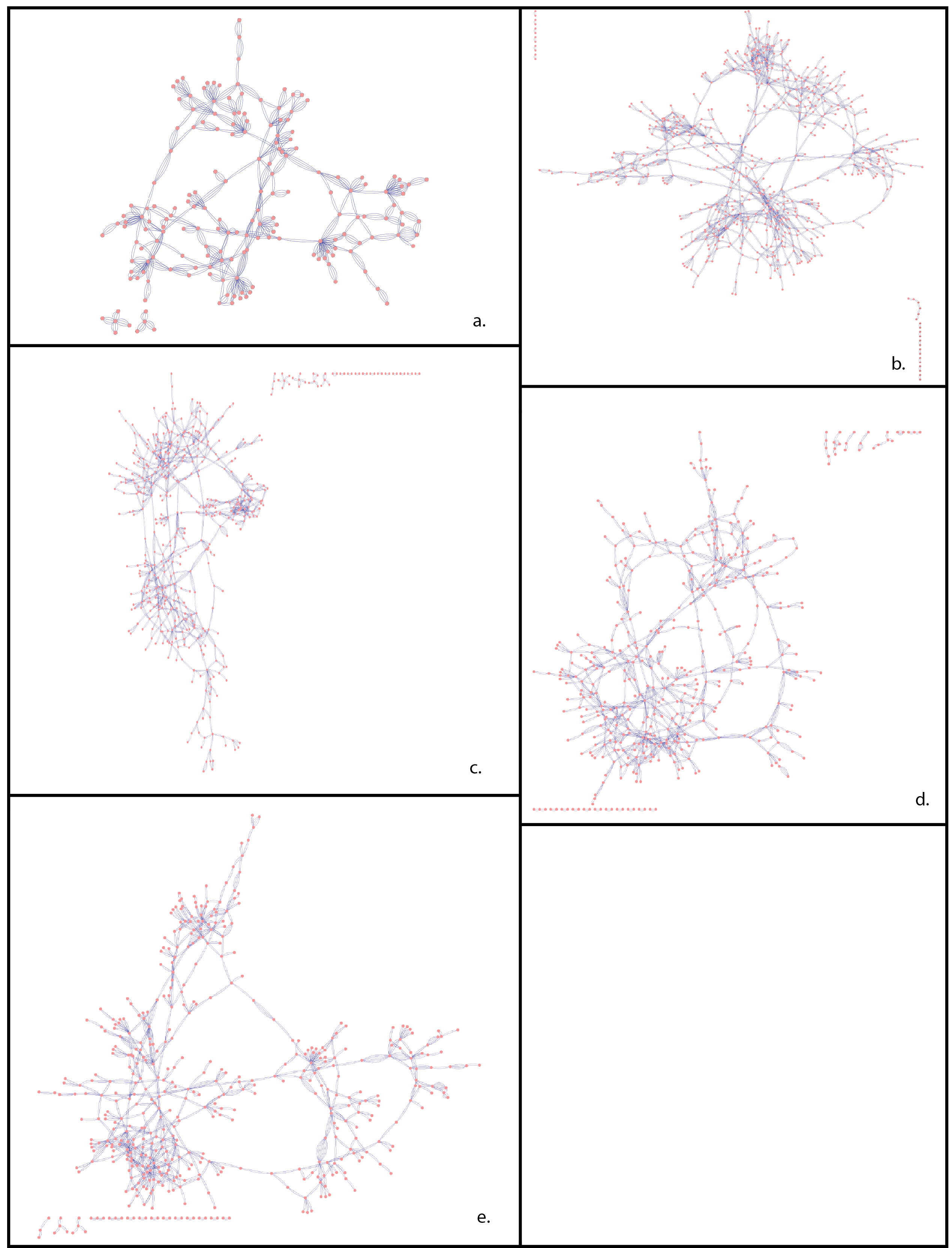

Figure 8. Example exchange networks, scenario 3. Pink dots represent households and blue lines represent an exchange. Multiple lines represent multiple exchanges for those households. a. year 600, b. year 1000, c. year 1100, d. year 1200, e. year 1300

Conclusions

6.1

In this paper we created a weight-based system for agent time allocation, resulting in specialization of production. This in turn required us to develop a system of barter so that agents could exchange the goods they variably produced. We explored two scenarios for such specialization. In one, agents are allowed to determine the degree of specialization based only on their economic state. In the second, they take into account both their economic state and a social influence from their neighbours. As expected, households became more specialized when they were "allowed" to do so. Agents also became increasingly co-resident (that is, more households co-reside within specific 200m × 200m cells in the simulation), exchanged more goods with each other, and achieved higher global population levels in either of the specialization scenarios than in Scenario 1.

6.2

The social networks formed from the two types of specialization displayed somewhat different characteristics. While both displayed increasing compartmentalization through time, Scenario 3 displayed a generally higher clustering coefficient. The social influence of agents in this simulation is important to facilitate the flow of goods throughout the system. Future research into the "wealth" of the hub nodes will help elucidate how these nodes supply the network.

6.3

As we begin to explore this new model using parameterizations more reasonable for our reference case—the Basketmaker III through Pueblo III periods in the central Mesa Verde region—we will investigate several questions raised by the analysis here. What are the spatial characteristics of the networks formed by the combination of specialization and barter? How do the sizes and locations of the communities discoverable in the model compare with those known from our study area? Does the combination of barter and specialization increase the sizes of the communities in the model, relative to communities discoverable from the networks generated by reciprocity among agents with largely redundant production?

6.4

Kohler, Herr and Root (2004) suggested that many of the differences between pre-AD 1280 in Southwest Colorado and the post-AD 1375 Pueblo societies in the northern Rio Grande can be attributed to the addition of proto-market forces to economies previously structured by economies based mostly on reciprocity. Abbott et al. (2007) suggested that in the Hohokam area in the deserts of southern Arizona, periodic marketplaces and barter in goods such as earthenware containers may be important structuring forces even earlier, by around AD 1000. Further work with this model will help us understand the extent to which differences in site and community sizes and locations can be legitimately attributed to the addition of barter and specialization to economies previously based on reciprocity.

6.5

In the models presented here we are engaging in counter-factual explorations, since it appears unlikely to us that the high degrees of specialization and large amounts of barter that typify our Scenarios 2 and 3 in fact characterized the economies of societies in southwestern Colorado between AD 600 and 1300, when the area we model was depopulated in a collapse that affected the entire northern Southwest. Assuming that this depopulation was not just due to a large external shock (which may in fact have been the case) we can use these models to guide our intuitions as to whether the pre-1300 societies in southwestern Colorado would have been more (or less) resistant to this collapse if they had in fact developed more specialization and barter.

6.6

In their recent review of the structural characteristics of systems approaching and undergoing critical transitions, Scheffer et al. (2012) propose that, in general, modularity and heterogeneity create more robust (less fragile) systems than do connectivity and homogeneity. In our model systems, it is true that specialization and barter lead to more connectivity among households, as pointed out in section 5.5, but on the other hand, those households are more heterogeneous than in the Scenario 1 case, where all households engage in the same suite of activities to approximately the same extent. So, while their high connectivity may make Scenario 2- and 3-type systems more prone to undergoing a critical transition such as collapse, their heterogeneity may provide some protection against that possibility. That the post-1300 Pueblo societies in the northern Rio Grande seem to have been highly stable in spite of their (presumed) high degree of connectivity may signal that heterogenetity is more fundamental to stability than is degree of connectivity. It is also possible that the agricultural systems developed in the northern Rio Grande—based on water management rather than rainfall—were so much more stable that any deleterious consequences for high connectivity were never expressed.

6.7

The next phase in this strand of VEP research will involve enlarging our study area to include both southwestern Colorado and the northern Rio Grande. This will provide us with an opportunity to see the extent to which the structure of the environment in the northern Rio Grande itself encourages the formation of specialization and barter, or whether the possibility of engaging in a single specialization (such as growing cotton, which was not possible throughout that area, or in southwestern Colorado) can provoke a cascade of other specializations in the model households.

Acknowledgements

This research was made possible by grant DEB-0816400 to Kohler, Craig Allen, Ziad Kobti, and Mark Varien. Crabtree also acknowledges support from grant DGE-080667. Crabtree and Kohler thank the Laboratoire Chrono-Environnement (UMR-6249) of the Maison des Sciences de l'Homme et de l'Environnement C.N. Ledoux and the Université of Franche-Comté of Besançon for support while completing final edits to this manuscript.

References

ABBOTT, D. R., Smith, A. M. and Gallaga, E. (2007). Ballcourts and ceramics: The case for Hohokam marketplaces in the Arizona desert. American Antiquity, 72(3), 461-484. [doi:10.2307/40035856]

ASSENOV, Y., Ramirez, F., Schelhorn, S. E., Lengauer, T. and Albrecht, M. (2008). Computing topological parameters of biological networks. Bioinformatics, 24(2), 282-284. [doi:10.1093/bioinformatics/btm554]

BASCOMPTE, J. (2010). Structure and dynamics of ecological networks. Science, 329, 765-766. [doi:10.1126/science.1194255]

BEAUDREAU, B. (2003). On the origins of large-scale specialization and exchange: A game-theoretical approach. In The Canadian Economic Theory Conference. Montreal, Canada.

BERNARDINI, W. (2000). Kiln firing groups: Inter-household economic collaboration and social organization in the northern American Southwest. American Antiquity, 65(2), 365-377. [doi:10.2307/2694064]

BESHERS, S. and FEWELL, J. (2001). Models of division of labor in social insects. Annual Review of Entomology, 46, 413-440. [doi:10.1146/annurev.ento.46.1.413]

BONNER, J. (1993). Dividing the labor in cells and societies. Current Science, 64, 459-466.

BONNER, J. (2004). Perspective: The size-complexity rule. Evolution, 58, 1883-1890. [doi:10.1111/j.0014-3820.2004.tb00476.x]

CHAI, L., Chen, J., Han, Z., Di, Z. and Fan, Y. (2007). Emergence of specialization from global optimizing evolution in a multi-agent system. In: International Conference on Computational Science, 4. [doi:10.1007/978-3-540-72590-9_13]

CHILDE, V. G. (1936/1983). Man Makes Himself. New York: New American Library.

COCKBURN, D. and KOBTI, Z. (2009a). Agent specialization in complex social swarms. Studies in Computational Intelligence, 248, 77-89. [doi:10.1007/978-3-642-04225-6_5]

COCKBURN, D. and KOBTI, Z. (2009b). The effect of social influence on agent specialization in small-world social networks. IEEE Congress on Evolutionary Computing, 3172-3175. [doi:10.1109/cec.2009.4983345]

COCKBURN, D. and KOBTI, Z. (2011). Wasps: A weight allocated social pressure system for agent specialization. European Conference on Artificial Life, Paris.

COCKBURN, D., Kobti, Z. and Kohler, T. A. (2010). A reinforcement learning model for economic agent specialization. In: FLAIRS Conference.

CRABTREE, S. A. (2012). Why can't we be friends? Exchange, alliances and aggregation on the Colorado Plateau. Unpublished Masters Thesis, Washington State University. Pullman, WA.

DALTON, G. (1982). Barter. Journal of Economic Issues, 16(1), 181-190.

DONCHEVA, N. T., Assenov, Y., Domingues, F. S., Albrecht, M._ (2012). Topological analysis and interactive visualization of biological networks and protein structures._ Nature Protocols, 7:670-685. [doi:10.1038/nprot.2012.004]

EPSTEIN, J. M. (2008). Why Model?. Journal of Artificial Societies and Social Simulation 11(4)12. https://www.jasss.org/11/4/12.html

EVANS, R. (1978). Early Craft Specialization: An Example for the Balkan Chalcolithic. In Social Archaeology: Beyond Subsistence and Dating. New York: Academic Press.

GORELICK, R., Bertram, S., Killeen, P. and Fewell, J. (2004). Normalized mutual entropy in biology: quantifying division of labor. American Naturalist 164, 678-682. [doi:10.1086/424968]

HARRY, K. G. (2005). Ceramic specialization and agricultural marginality: Do ethnographic models explain the development of specialized pottery production in the prehistoric American Southwest? American Antiquity, 70(2), 295-319. [doi:10.2307/40035705]

HEGMON, M. (1989). Risk reduction and variation in agricultural economies: A computer simulation of Hopi agriculture. Research in Economic Anthropology, 11, 89-121.

JEANSON, R., Fewell, J., Gorelick, R. and Bertram, S. (2007). Emergence of increased division of labor as a function of group size. Behavioral Ecology and Sociobiology. 62, 289-298. [doi:10.1007/s00265-007-0464-5]

KOBTI, Z. and Reynolds, R. (2005). Modeling protein exchange across the social network in the village multi-agent simulation. In: Systems, Man and Cybernetics, 2005 IEEE International Conference ON, 4, 3197-3203. [doi:10.1109/icsmc.2005.1571638]

KOBTI, Z., Reynolds, R. and Kohler, T. (2004). The effect of kinship cooperation learning strategy and culture on the resilience of social systems in the village multi-agent simulation. In: Evolutionary Computation, 2004. CEC 2004 Congress ON, 2, 1743-1750. [doi:10.1109/cec.2004.1331106]

KOHLER, T. A., Herr, S., and Root, M. J. (2004). The Rise and Fall of Towns on the Pajarito (A.D. 1375-1600). In Kohler, T. A. (Ed) Archaeology of Bandelier National Monument: Village Formation on the Pajarito Plateau (pp. 215-264). University of New Mexico Press.

KOHLER, T., Johnson, C. D., Varien, M. D., Ortman, S., Reynolds, R., Kobti, Z., Cowan, J., Kolm, K., Smith, S. and Yap, L. Y. L. (2007). Settlement Ecodynamics in the Prehispanic Central Mesa Verde Region. In Kohler, T. A., Van der Leeuw (Eds.) The Model-Based Archaeology of Socionatural Systems (pp. 61-104). Santa Fe, New Mexico: SAR Press.

KOHLER, T.A. Kresl, J., van West, C., Carr, E. and Wilshusen, R. H. (2000). Be There Then: A Modeling Approach to Settlement Determinants and Spatial Efficiency among Late Ancestral Pueblo Populations of the Mesa Verde Region, U. S. Southwest. In Kohler, T.A., Gumerman, G. G. (Eds.) Dynamics in Human and Primate Societies: Agent-based Modeling of Social and Spatial Processes (pp. 145-178). Santa Fe Institute and Oxford University Press.

KOHLER, T. A., Varien, M. D., Wright, A. and Kuckelman, K. A. (2008). Mesa Verde migrations: New archaeological research and computer simulation suggest why Ancestral Puebloans deserted the northern Southwest United States. American Scientist 96,146-153. [doi:10.1511/2008.70.3641]

KOHLER, T. A. (2012) Modeling Agricultural Productivity and Farming Effort. In T. A. Kohler and M. D. Varien (Eds.) Emergence and Collapse of Early Villages: Models of Central Mesa Verde Archaeology (pp. 85-111). University of California Press, Berkeley. [doi:10.1525/california/9780520270145.003.0006]

KOHLER, T. A., M. D. Varien (eds.) (2012). Emergence and Collapse of Early Villages: Models of Central Mesa Verde Archaeology. University of California Press, Berkeley. [doi:10.1525/california/9780520270145.001.0001]

KRINK, T., Mayoh, B. and Michalewicz, Z. (1999). A patchwork model for evolutionary algorithms with structured and variable size populations. In Genetic and Evolutionary Computation Conference.

LAVEZZI, A. M. (2003). Complex dynamics in a simple model of economic specialization. Computing in Economics and Finance 2003 170, Society for Computational Economics.

LIPE, W. D., Varien, M. D., and Wilshusen, R. W. (ed.) (1999). Colorado Prehistory: A Context for the Southern Colorado River Basin. Colorado Council of Professional Archaeologists.

MURCIANO, A. M. and Zamora, J. (1997). Specialization in multi-agent systems through learning. Biological Cybernetics 76(5), 375-82. [doi:10.1007/s004220050351]

NEWMAN, M. E. J. (2010). Networks: An Introduction. Oxford University Press, USA. [doi:10.1093/acprof:oso/9780199206650.001.0001]

ORTMAN, S. (2003). Artifacts. In The Archaeology of Yellow Jacket Pueblo: Excavations at a Large Community Center in Southwestern Colorado. http://www.crowcanyon.org/researchreports/yellowjacket/text/yjpw_artifacts.asp

PATTERSON, T. C. (2005). Craft specialization, the reorganization of production relations and state formation. Journal of Social Archaeology 5, 307-337. [doi:10.1177/1469605305057570]

RAVARY, F., Lecoutey, E., Kaminski, G., Châline, N. and Jaisson, P. (2007). Individual experience alone can generate lasting division of labor in ants. Current Biology. 17(15), 1308-1312. [doi:10.1016/j.cub.2007.06.047]

REYNOLDS, R., Kobti, Z. and Kohler, T. (2004). The effects of generalized reciprocal exchange on the resilience of social networks. Computational and Mathematical Organizational Theory 9, 227-254. [doi:10.1023/B:CMOT.0000026583.03782.60]

REYNOLDS, R.G., Kobti, Z., Kohler, T.A., and Yap, L. Y. L. (2005). Unraveling Ancient Mysteries: Reimagining the Past Using Evolutionary Computation in a Complex Gaming Environment. IEEE Transactions on Evolutionary Computation 9:707- 720. [doi:10.1109/TEVC.2005.856206]

SAHLINS, M. (1972). Stone Age Economics. Aldine Atherton.

SCHEFFER, M., Carpenter, S. R., Lenton, T. M., Bascompte, J., Brock, W., Dakos, V., van de Koppel, J., van de Leemput, I. A., Levin, S. A., van Nes, E. H., Pascual, M., and Vandermeer, J. (2012). Anticipating Critical Transitions. Science 338 (6105), 344-348. [doi:10.1126/science.1225244]

SHANNON, C. (1948). A mathematical theory of communication. Bell System Technical Journal 27, 379-423, 623-656. [doi:10.1002/j.1538-7305.1948.tb00917.x]

SMITH, A. (1776/1937). An Inquiry into the Nature and Causes of the Wealth of Nations. Modern Library.

SPENCER, A. J., Couzin, I. D. and Franks, N. (1998). The dynamics of specialization and generalization within biological populations. Journal of Complex Systems, 1(1), 115-127. [doi:10.1142/S0219525998000077]

THERAULAZ, G., Bonabeau, E. and Deneubourg, J. (1998). Response threshold reinforcements and division of labour in insect societies. In Proceedings of the Royal Society B Biological Sciences, 265(1393), 327-332. [doi:10.1098/rspb.1998.0299]

VAN VUGT, M. and Ahuja, A. (2011). Naturally Selected: The Evolutionary Science of Leadership. HarperBusiness, New York.

VAN WEST, C. R. (1994). Modeling prehistoric agricultural productivity in Southwestern Colorado: A GIS approach. Reports of investigations NO. 67. Department of Anthropology, Washington State University, Pullman, and, Crow Canyon Archaeological Center, Cortez, CO.

VARIEN, M. D., Ortman, S. G., Kohler, T. A., Glowacki, D. M. and Johnson, C. D. (2007). Historical ecology in the Mesa Verde region: Results from the Village Ecodynamics Project. American Antiquity, 72(2), 273-300. [doi:10.2307/40035814]

WAIBEL, M., Floreano, D., Magnenat, S. and Keller, L. (2006). Division of labour and colony efficiency in social insects: effects of interactions between genetic architecture, colony kin structure and rate of perturbations. Biological Society, 273, 1815-1823. [doi:10.1098/rspb.2006.3513]

YOUNG, A. A. (1928). Increasing returns and economic progress. The Economic Journal 38, 527-542. [doi:10.2307/2224097]

Appendix - Formal Problem Description and Approach

Problem Description

Given agent Ag, the set tAG and a resource rAG, how does an agent allocate its rAG among each task t in tAG?

So: Σ x_i=S(R_Ag)
where i is each task in tAG , S(rAG) refers to the amount of the resource rAG available, and x_i refers to a fraction of S(rAG).

The problem also involves the following conditions:
The problem is continuous over a period of iterations
S(rAG) changes between iterations
x_i is allowed to change over iterations
Each agent Ag also has a set REQ(Ag), such that a resource r in REQ (Ag) needs some amount of r for subsistence between iterations.

Weight-based model for time allocation among tasks

We used a weight-based approach for agents' time allocation based on Cockburn and Kobti's study (2011). A quick summary of that approach (named WASPS) is presented here.

For each agent Ag, we propose a set EC, where e_i in EC. There is a task i in tAG and e_i represents the weight of task i.

Task weights in EC are relative, therefore for the given a task i and a resource to be allocated rAG, the amount of rAG to be allocated to task i is:
e_i/S(EC) × S(rAG)
where S(EC) is the sum of all elements in EC.
We make no assumptions about the initialization of the weights in EC. They can be randomly assigned, or initialized by some other method. A task having a weight of 0 will result in the task being allocated none of rAG.
Ag must possess some evaluation function P(t) for each task t in EC.
P(t) is assumed to be a composite function, assumed to be an economic performance function.
P(t) is applied to each task in EC after the performance of that task, therefore representing the result of performing the task.
If P(t) > 0, the task is assumed to have had a positive result, in which case e_t is increased by some factor, which is domain dependent. In the case of P(t) < 0, e_t is similarly decreased by some factor. The result of this process is the updating of the weights in EC, which in turn determine how each agent allocates the resource in question. More details on the methodology can be found in Cockburn and Kobti (2011)