Abstract

The purpose of this study is to model and analyze by simulation the dynamics of endogenously created oscillations in real estate (housing) prices. A system dynamics simulation model is built to understand some of the structural sources of cycles in the key housing market variables, from the perspective of construction companies. The model focuses on the economic balance dynamics between supply and demand. Because of the unavoidable delays in the perception of the real estate market conditions and construction of new buildings, prices and related market variables exhibit strong oscillations. Two policies are tested to reduce the oscillations: decreasing the construction time, and taking into account the houses under construction in starting new projects. Both policies yield significantly reduced oscillations, more stable behaviors.

Keywords:

Real Estate Modeling, Housing Cycles, Price Oscillations, System Dynamics, Socio-Economic Simulation

Introduction

1.1

Real estate market in general, housing in particular is one of the most dynamic and unpredictable economic sectors (Hiang & Webb 2007; Mu et al. 2009). Moreover, the real estate sector involves large and influential investments, thus affecting the whole economy and the labor market profoundly. Typically, housing markets exhibit oscillatory behaviors, with cycle periods ranging from a few years to a few decades (Wheaton 1999). As will be seen in the literature review below, endogenous structure of the housing sector itself can play a significant role in the creation of such cycles: A positive housing demand movement causes the prices to rise (Aoki et al. 2004). Even after new constructions, the prices may continue to rise, since expectations are formed by past movements in the prices. The prices peak when constructions overshoot the demand, at which point the prices start to decline. This process sets off a repeating cycle in the prices, construction, and the stock of houses. Within this dynamic environment, construction companies face a great risk of loss (or a chance of profit) due to the oscillatory behavior of the prices. If they just react to the prices and start or phase out their projects accordingly, they may have unsold houses in the bust times or not enough houses in the boom times. Because of the unavoidable delays in the system, companies must foresee the demand movements and start their projects well before the demand starts rising. The increase in the population growth makes the market even more complex and harder to predict (Genta 1989; DiPasquale & Wheaton 1994; Aoki et al. 2004; Sæther 2008).

1.2

Additional to its economic dynamics, housing development is a process that operates as a connected sequence of events. These series of events (i.e. site identification, feasibility analysis, design, production and occupation) transform a vacant site or a redundant or obsolete property into a new use. Through this development process many different actors and institutions such as developers, owners, occupiers, lenders, contractors and sub-contractors, architects, technologists, local government, consultants, engineers play different roles (Wyatt 2007). Inevitably, these operations and players are affected by many different factors such as long-term social trends, national and global economic conditions, environmental amenities, and government policies (Wyatt 2007; Selim 2009). Similarly economic crisis and global economic recessions have different effects on real estate markets in US and Europe (Deloitte 2010). The parameters and assumptions of our study are derived from Turkey where real estate market is growing with speed (Binay & Salman 2008). According to Keskin (2008) housing prices are affected by house size, level and age of the building and safety (especially earthquake risk) and security of the site, average income, time spent in the city and neighbor satisfaction. In addition to these determinants other housing market variables, rapid urbanization and urban population growth strengthen the housing market in Turkey (Coskun 2011).

1.3

Due to the dynamic stock-flow nature of the housing variables, stock-flow models of housing sector have been widely used since 1960s (DiPasquale & Wheaton 1994; Fair 1972; Maisel 1963). The common feature of these models is that they represent the relationships between the housing stocks and their flows by difference/differential equations. Most of these models are used to reflect the physical conversion process of constructions to house supply. However, this physical process is only a part of the system. In studies that model only a part of the system, the dynamics and forecasts have to be based on variables exogenous to the model. The majority of the studies in the housing literature build econometric models based on this stock-flow structure that seek to explain or forecast exogenously the dynamics of the system variables. Over the years, many improvements have been made in stock-flow modeling, by using evidence from literature and representing more variables endogenously in the model. As will be seen below, there is a thread of literature that seeks to explain the market behavior almost endogenously based on more elaborate stock-flow models. Our study belongs in this branch of literature, by adopting a "systems" perspective to the problem of housing price cycles. It means that we focus on how system components, in this case, the supply, demand and price, related decisions and delays, all interact with each other. Instead of seeing the problem as an open system that is determined by external forces, we identify feedback loops between the system variables, to explain the oscillations. These feedback loops include not only the physical processes like construction or price adjustment, but also the mental processes of decision makers, like effect of price on new construction decisions or perception formations. To formally represent these processes, we use system dynamics methodology, a modeling and simulation discipline that uses multiple stock-flow structures and feedback loops to analyze complex socio-economic dynamic systems (Forrester 1961; Sterman 2000).

1.4

System dynamics uses stock and flow variables to denote the processes that can be expressed by a differential (or difference) equation: the rate of change of a stock is the net sum of its flows. The stocks change through their flows, and the flows can be functions of any variables in the model. Stocks are used to represent not only physical accumulations (like stock of houses), but also intangible accumulations (like expectations that develop over time). One of the unique features of system dynamics approach is that it holds a systemic (holistic) worldview. This systemic perspective means striving to build models that incorporate endogenously all variables that are relevant to the problem. Thus, the outputs of the model are driven not by the external factors, but by the internal structure of the model. The internal structure comprises the feedback loops formed by interdependencies between variables.

1.5

Our model builds upon previous stock-flow models of housing markets, as well as generic structures used in system dynamics literature to represent common physical and mental processes. It is a dynamic model of the demand and supply sides of the real estate market in a major and still growing city. The model is a generic one and likely to be reasonably valid for any developing urban area. However, the parameters and assumptions are based on the city of Istanbul, Turkey.

1.6

In Section 2 of the paper, a literature review of the related studies is presented. Then, the methodology is described in Section 3. In Section 4, the model is explained and the validation process is summarized. Finally, scenario and policy analysis results are presented.

Literature Review

2.1

Our model is a continuous time, nonlinear, non-equilibrium, dynamic stock-flow model that consists of feedbacks in both supply and demand sides of the system. The model particularly focuses on endogenously created cycles of housing market in the long term from the constructor company perspective. Although current literature includes many models that possess one or many of these properties, our model is unique in the sense that it combines all these aspects.

2.2

Price is one of the key variables of the housing sector, as well as our model. Causal mechanisms that drive the housing price dynamics, which constitute the core of our model, have been subject of many model-based studies in the past 50 years. Anas (1978) develops a recursive dynamic model of urban residential growth. The model focuses on how consumption, housing prices, and land rents adjust over time. In a study that is not housing-specific, Fershtman and Fishman (1992) uses a dynamic search model to demonstrate that the price of a commodity can show cyclical behavior due to endogenous dynamic interactions between buyers and firms, without any external intervention to the system. Chicago Prototype Housing Market Model presented in Anas and Arnott (1993) is a multi-dimensional, discrete-time, dynamic equilibrium model that reflects asset bid-price, housing stock adjustment and market clearing processes. It is a policy-oriented model with a medium term time horizon (10 years) focusing mainly on the dynamics of the subcomponents of the system. Meen (2000) develops a mathematical model including house prices, constructions, cost and interest rates and their interactions to analyze housing cycles of the UK market. Filatova et al. (2009) develops an agent-based model that includes behavioral drivers of land-market transactions on both the buyer and seller sides. Murphy (2010) presents a dynamic micro-econometric model of housing supply to explain the volatility in prices in the San Francisco Bay Area.

2.3

Among the dynamic models of housing market, the stock-flow models are of particular interest to us (as explained in Section 3). A study can be classified as stock-flow model if it has a conceptualization of the system based on stock and flows in a dynamic perspective. In one of the early studies, Maisel (1963) presents a model with two basic stocks: stock of dwellings and inventory under construction, which are connected through completions flow. The inflow, called starts, is determined by builders, by taking into account the stock and some external factors. This is a rather simple framework focusing mainly on the supply side of the system. Smith (1969) uses a similar structure for the housing market, but presents a more elaborate model of the mortgage market and relates to the demand side of the housing market. However, the model does not include separate supply and demand equations, meaning that equilibrium is assumed. Fair (1972) summarizes a few other models that assume equilibrium between demand and supply.

2.4

Weibull (1983) presents a three-stock structure to represent demand, supply and price in a continuous-time dynamic model. The model accounts for nonlinearities present in the system, but lacks the construction and investment side of the problem. Poterba (1984) uses a model composed of two differential equations for housing stock and price. Although this model represents price endogenously, it lacks some related delays and feedback loops. The paper by DiPasquale and Wheaton (1994) provides a summary of historical development of stock-flow based housing models and develops a dynamic stock-flow model of housing market to understand its aggregate behavior. Authors also improve the earlier stock-flow models by including gradual price adjustment, expectation formation and a feedback loop controlling new constructions. Although this model reflects the essential backbone of a dynamic housing model, there is only one major feedback loop, which is from housing stock to the construction starts through price. The model developed by DiPasquale and Wheaton (1994) has been modified by Tu (2004) and applied to Singapore private housing market. Jiang et al. (2010) also modifies the stock-flow model of DiPasquale and Wheaton (1994) to analyze the factors driving housing market cycles in China. Yet these modifications do not enrich the model structure but merely adapt the model to different locations.

2.5

Although the aforementioned studies use a stock-flow structure they are essentially data-driven, exogenous models that seek to explain and predict price fluctuations. Some studies, on the other hand, use endogenous stock-flow structures to generate the dynamic behavior of the housing market. For instance, Barras (2005) builds a set of difference equations to explain endogenously the cyclical behavior housing market. The model accounts for two types of demand creation: due to growth and due to turnover. There are delay structures in rent (or price) adjustment, occupier response to rent changes, construction starts, and construction completions. However, this model ignores the effect of price on demand and the matching process between supply and demand. Likewise, Eskinazi et al. (2011) creates a system dynamics model for the Netherlands housing market based on DiPasquale and Wheaton model.

2.6

There are other examples of housing-related studies in the system dynamics literature. J. Forrester's Urban Dynamics model (1970) is one of the first system dynamics models dealing with the housing dynamics in an urban area. It focuses on the connections between the labor, business and housing sectors, but does not include variables about price. Recently, Kummerow (1999) presents a system dynamics model for cyclical office oversupply problem. His model consists of a single balancing feedback loop between vacancy rate and supply, assuming all other factors external. The paper asserts that the supply lag, the adjustment time and the tendency of oversupply are responsible for the cycles and they can serve as leverage variables for reducing the cycles. Hong-Minh and Strohhecker (2002) presents a system dynamics model for the private housing supply chains to assess the impact of re-engineering scenarios on construction performance and to study the impact of re-engineering policies on demand amplifications. Ho et al. (2010) presents a model of housing market of Taichung City in Taiwan to determine the effectiveness of various government policies. Genta (1989) and Sæther (2008) develop system dynamics models to explain the housing cycles in Boston and Norway, respectively.

2.7

One distinctive property of our model is its endogenous focus. In our study, like other system dynamics-based studies, we mainly focus on the dynamics generated by the interactions between the system variables. As a system dynamics model, its dynamic behaviors are endogenously generated, rather than being externally data-driven. The aim is not to forecast the house prices at specific time points, but to understand how and why the price cycles occur. The model is not only valid for the equilibrium state but has the capability to reflect the transient dynamics in the housing market.

2.8

Unlike the system dynamics models cited above, our model is built from the perspective of construction companies. The problem owner is important because it determines the model boundary. Since our model is constructer-oriented, it involves economic decision-making processes of the companies. Due to the fact that construction companies do not have direct influence on households' buying decisions, the demand side and the purchasing power of the customers are modeled in less detail. The problem perspective is also relevant in identifying feasible policy interventions and evaluating their outcomes. Our recommended policies modify decision parameters that are under control of construction sector, and the evaluation of these policies considers their effects on profits.

2.9

Structure-wise, our model also brings several improvements to the existing models in the literature. The traditional assumption in the stock-flow model is that the market clears quickly (DiPasquale and Wheaton 1994). However, the price adjustment mechanism and the search process can cause significant time lags that can affect the dynamic behavior. Although gradual price adjustment is a feature of some earlier models (for example, DiPasquale & Wheaton 1994; Barras 2005; Eskinazi et al. 2011), no other model that we reviewed explicitly models the search process and its effect on sales duration. Moreover, many models either assume demand to be external (Maisel 1963; Kummerow 1999; Sæther 2008), or solely dependent on supply (Barras 2005; Jiang et al. 2010), ignoring the effect of price on demand. By including all these feedback loops, a rich structure is created which is capable of producing different behaviors endogenously.

Methodology

3.1

System dynamics is a model-based methodology to analyze complex dynamic systems involving feedback interactions. The basic elements of a system dynamics model are stocks and flows. A stock variable represents an entity that gradually accumulates or diminishes over time. A flow is the rate of change of a stock. Mathematically, the relationship between stocks and flows corresponds to differential (or difference) equations. Apart from stocks and flows, there are auxiliary variables that represent the stock-to-flow links explicitly. Feedback corresponds to a situation where X influences Y, and Y in turn influences X through a chain of causal relationships. There are two types of feedback loops; a positive feedback loop means that an initial change (increase or decrease) in a variable will eventually cause the same variable to change in the same direction. On the contrary, a negative feedback loop has a balancing effect: an initial change in a variable will eventually cause the same variable to change in the opposite direction (See Figure 2 for an illustration of feedback loops). Since variables in a system are interconnected through feedback loops, the behavior of any variable is dependent on the whole system. For more information on system dynamics methodology see, for instance, Barlas (2002) and Sterman (2000).

3.2

The motivation of this study is to investigate the structural reasons behind the cyclic behavior of the main housing variables. The model boundary is selected large enough to make sure the causal mechanisms that drive the system behavior lie inside the boundary, as suggested in system dynamics literature (Forrester 1987). The dynamic hypothesis is presented using a causal-loop diagram (Figure 2), which explains how variables are linked to each other. This conceptual model is then translated to a formal mathematical model in the form of a stock-flow diagram and equations (Figure 3). After verification and validation steps, the causes of the oscillatory behavior can be identified by a series of simulation experiments. With the aid of such a model, it is possible to design improvement policies to dampen the oscillations and analyze their effects on the whole system.

3.3

The model is developed and implemented using STELLA 9.1.4 (isee systems 2009). In STELLA and most computer simulation applications of system dynamics models, the dynamic relationships between the elements, including variables, parameters, and external inputs, are captured in the interface in forms of equations, graphs and functions (as given in Appendix) using user-friendly visual tools. It is a flexible way for building simulation models from causal loops or stocks and flows. When simulation runs are carried out, various types of graphs and tables are the outputs from STELLA. The model can be downloaded from: http://www.openabm.org/model/3936/.

The Model

4.1

The model is built from the perspective of the construction companies. Specifically, the decision maker could be a trade chamber, an association or a consortium of construction companies. So, the model focuses on the construction chains and the decision-making processes of the companies. This dynamic model seeks to explain the structural causes of housing market oscillations and test alternative policies that may improve the decision making process of the construction companies.

4.2

The real estate prices are known to exhibit oscillatory behaviors in real life (Wheaton 1999). In Figure 1, the de-trended ratio of real estate rent index to the overall price index in Istanbul is used as a reference behavior for the model. The rent prices are used as a reference because long-term house price data series for Istanbul is not available. Rent and house prices in Istanbul are in general assumed to be strongly correlated, which logically makes sense. Moreover the strong linkage between rents and prices in housing is also shown in the literature (Hargreaves 2008; Gallin 2008). We believe that the behavior of the rent price is a good proxy for the real estate price behavior for Istanbul.

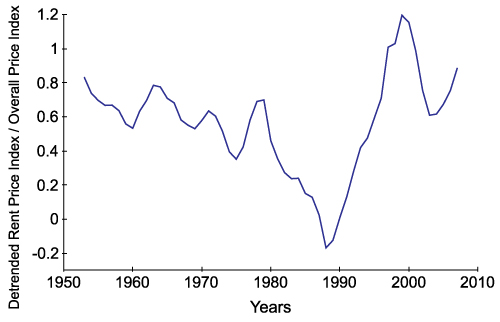
Figure 1. A reference behavior for the model: The line represents the de-trended ratio of real estate rent index to the overall price index in Istanbul

4.3

The time unit of the model is in years since the major time delays and the rates of changes are measured in terms of years. The time horizon is 60 years between 1970 and 2030. The motivation for selecting a long range is to be able to observe at least a few cycles.

4.4

The model includes the following elements; the houses under construction, for sale, and sold; the demand for houses; the price, and the profit. The city population continuously increases with immigration and births, which is taken as an external input to the model. The cost of building houses is also modeled as an input that changes over time. The effect of national economy on the construction companies is not considered. We also assumed that there is practically no land limitation for building new houses. There is an upper bound for the construction rate, which reflects the constraints on the labor, capital and other resource limitations for the constructors. The parameter values in the model are mostly based on rough estimates due to lack of statistical data regarding these parameters. Since this model does not aim to forecast the specific values of variables in the market, our focus has been structural validity rather than numeric precision of the parameters.

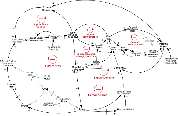
Figure 2. The causal loop diagram of the model

Model Structure

4.5

The causal loop diagram shown in Figure 2 presents the interactions between variables that constitute the engine behind the oscillatory dynamics. Since the causal loop diagram is a qualitative description of the system's feedback structure, it shows only the major variables. Arrows show how the variables affect each other ceteris paribus. An arrow with a positive sign means that a change in X causes Y to change in the same direction, other things being equal. A negative influence means a change in X causes Y to change in the opposite direction. The || sign implies a delay before an effect reaches a variable. Figure 3 shows the stock-flow diagram of the model. Stock-flow diagram corresponds to the formal quantitative model used in simulations. Each variable has a corresponding equation in the Appendix.

4.6

In the remaining part of this section, we explain major feedback loops and critical formulations. We refer readers to the causal-loop diagram (Figure 2) when feedback loops are discussed, and to the stock-flow diagram (Figure 3) when specific formulations are discussed.

4.7

Three major balancing (negative) feedback loops govern the behavior of the system, as will be described below: demand-price, supply-price and supply-demand loops. A balancing loop counteracts any disturbance in variables in the loop, forcing the system to seek an equilibrium.

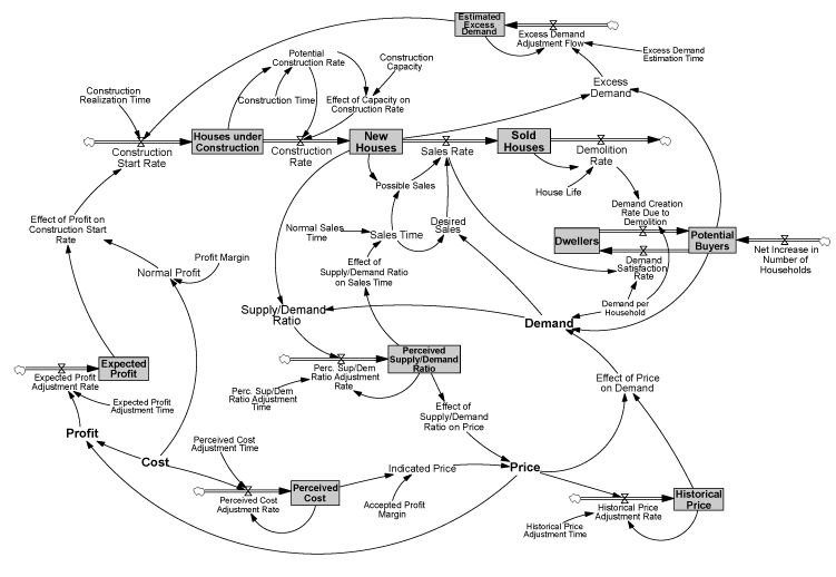
Figure 3. The stock-flow diagram of the model. Rectangles stand for the stocks and pipes with valves stand for the flows. Other variables are auxiliaries or parameters.

The life cycle of houses

4.8

Like most stock-flow models, our model represents the life cycle of houses by a series of stocks variables: houses under construction, new houses, and sold houses (Maisel 1963). Two flow variables connect the stocks: construction rate and sales rate. Construction rate is limited by construction capacity, which is a result of physical resource limitations. The new projects first turn into constructions and then to new houses after a construction delay.

4.9

Sales rate is dependent on both supply and demand. Sold houses are demolished after an average lifetime of 40 years.

Demand creation process

4.10

In the model, potential buyers is a stock variable that represents the households who need a house for dwelling (see Figure 3). New potential buyers are created by two ways: demand created due to demolition (natural turnover) and increase in number of households (demand creation due to population growth) (Barras 2005). Potential buyers stock decreases by demand satisfaction rate (which is equal to the sales rate). This stock and its flows are thus defined in the following differential equation:

d(Potential Buyers)/dt = Net increase in number of households +    Demand creation rate due to demolition − Demand satisfaction rate

(1)

The differential equations show the continuous rate of change of the stocks. In order to evaluate them in computer simulation, a small time step (dt) is used to compute the value of the stock. Its value at time t+dt is computed iteratively as follows:

Potential Buyers t+dt = Potential Buyers t + (Net increase in number of households    + Demand creation rate due to demolition − Demand satisfaction rate) × dt

(2)

The above form of simulation equation holds in general for all stock equations.

4.11

Net increase in number of households shows the number of new houses demanded by the population (households) annually. It is an external input as given in Figure 4, based on historic household increase rates of Istanbul under the assumption that one household creates one house demand under normal price conditions. The future values are extrapolated based on current trend.

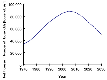
Figure 4. Net Increase in Number of Households over time (model input).

4.12

While variable potential buyers represents the population needing a house for dwelling, it is not necessarily equal to the actual demand on the market. The prevailing market price has an effect on the demand. Specifically, demand is dependent on effect of price on demand and potential buyers as shown Equation 3.

Demand = Potential buyers × Effect of price on demand

(3)

4.13

Effect of price on demand is a decreasing function of price and historical price as illustrated in Figure 5. When the average house price is higher than historical price, people tend to decrease the demand or vice versa. When price is equal to historical price, the effect function takes the value of 1. This makes demand equal to potential buyers, the normal demand level.

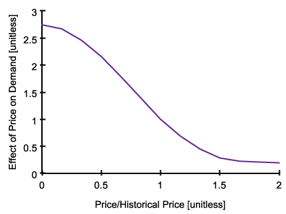
Figure 5. Effect of Price on Demand

4.14

Such nonlinear effect formulations are used throughout the model to express causal relations between variables. The advantage of using effect functions is the freedom to express any kind of nonlinear relation without being limited by certain hard-to-present/understand mathematical expressions.

Demand-Price loop

4.15

This loop reflects the classical balancing process of demand through price (See Figure 2). Suppose that at some given time the system is in equilibrium and demand suddenly increases (maybe due to a sudden immigration). This rise in demand decreases supply/demand ratio. Since it takes some time for market actors to perceive and respond to this change, price increases, after a delay. We used a first-order information delay structure to represent this process, which is widely used in system-dynamics literature (Sterman 2000) to model delayed perceptions (see Appendix). Increased price causes demand to fall back. A similar logical sequence of successive effects also holds for an initial decrease of demand, as well as any other variable in the loop.

Construction start process

4.16

Cost is taken to be an external input that changes with economic conditions, which are not explicitly included in the model, as given by Figure 6.

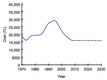
Figure 6. Average cost of dwelling units (model input)

4.17

The cost data are based on 1970–2008 statistics of average cost of dwelling units in Turkey, provided by Turkish Statistical Institute. The data are deflated to year 2009 prices and smoothed by nonparametric regression to avoid sudden changes in the model.

4.18

The difference between price and cost determines profit. As demonstrated by Kenny (1999), construction companies pass any increase in the costs to the buyers, in order to maintain profit margins. This fact is reflected in our model as normal profit that depends on cost and profit margin. Normal profit is the benchmark value for profit, used to compare the attractiveness of the profit obtainable by starting new projects (see Figure 3). The ratio of expected profit to normal profit determines effect of profit on construction start rate, which is a concave increasing function, similar to Figure 7. The difference between new houses and potential buyers is excess demand, as shown below.

Excess Demand = Potential Buyers − New Houses

(4)

This excess demand cannot be known accurately and the construction firms estimate it by an exponential smoothing process.

4.19

While Barras (2005) models the construction process as a stock-adjustment structure with a desired level of building stock (occupied or not) that change with economic growth, our approach reflects the constructor point of view. In our model, instead of trying to reach a desired housing stock, the firms aim to meet estimated excess demand by starting new constructions. If they expect a higher profit than their normal profits, their willingness to meet excess demand increases. The new projects turn into constructions and after a construction delay, to new houses and then demolishes. Construction rate is limited by construction capacity, which represents the constraints of available resources.

Supply-Price loop

4.20

Another major loop is the supply-price feedback loop (see Figure 2). When price rises, profit increases. Increased profit gradually increases expected profit. Companies compare their expected profit with normal profit (since companies cannot know the exact profit that can be obtained, an information delay structure is used to represent the profit expectation process of the firms). If expected profit is higher than normal profit, construction start rate rises. Through the physical process of construction, houses under construction yield new houses. The increased stock of new houses (the supply) increases the supply/demand ratio. The rise of supply/demand ratio creates a reduction in price. This is a negative feedback loop involving several delays. Although eventually any price change is compensated by the effect of new constructions, the delays slow down the process and cause the price to oscillate.

Supply stock control loop

4.21

There is a negative loop between the excess demand and the supply (see Figure 2). As explained above, estimated excess demand stimulates new constructions and the new houses for sale. This construction decreases the excess demand, which closes the balancing feedback loop. This loop is analogous to an inventory control structure that tries to keep the inventory constant at a target. In our model, inventory corresponds to new houses and target is the number of potential buyers.

Price

4.22

Price is anchored on indicated cost and adjusted by effect of supply/demand ratio on price (See Figure 3). Indicated price is the expected average price of a house under normal supply/demand conditions. It is assumed that, indicated price is 10% higher than the perceived cost of building a house. Perceived cost is the smoothed version of the average building cost in the market. Kenny (1999) demonstrated that house prices adjust positively in response to any excess demand for housing. In line with that observation, Effect of supply/demand ratio on price is modeled as a decreasing S-shaped function (see Appendix) similar to the formulations available in the literature (Genta 1989).

Sales Process

4.23

Sales occur when new houses and demand are both available. Search theory regards residential housing market as a sampling process of available houses with constant rate, which continue until buyer finds an acceptable house (Haurin 1988). Thus, the availability of houses relative to the demand determines the speed of sales, which is quantified in our model as follows:

Sales time = Normal Sales time × Effect of supply/demand ratio on sales time

(5)

4.24

Normal sales time (1 year) is the average time spent in matching the demand and the supply under normal market conditions. Effect of supply/demand ratio on sales time is an increasing concave function of 1/perceived supply demand ratio as given in Figure 7. It is assumed that if perceived supply/demand ratio decreases, sales time increases since it takes longer time for people to find a new house meeting their needs (as the probability of finding a match decreases).

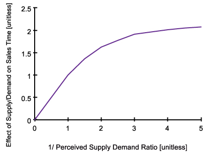
Figure 7. Effect of Supply/Demand Ratio on Sales Time

4.25

Possible sales is the average rate at which new houses can be sold in current sales time, without taking the demand into consideration. Desired sales, on the other hand, is the average rate at which demand can be met, ignoring the supply. Sales rate is the realized rate of sales, which is the minimum of desired and possible sales rates.

Supply-Demand Loop

4.26

This loop represents the balancing process between supply and demand, through sales and price (See Figure 2). As demand increases sales rate rises. This reduces the supply and raises price, after a delay. The risen price has a negative effect on demand.

Supply and Demand Self-Correction Loops

4.27

These are minor natural feedback loops that are results of stocks controlling their outflows. Increased supply of houses gives rise to faster sales, which in turn decreases the supply itself. A similar process works for the demand.

Supply Adjustment through Sales Time

4.28

This loop constitutes an extra balancing process for the new houses stock (see Figures 2 and 3). When the level of new houses becomes larger than the demand, the increased availability of new houses shortens the process of supply-demand matching, thus shortens the sales time. Decreased sales time leads to increased desired sales and possible sales, which means higher sales rate, which in turn balances off the rise in the new houses stock. Thus any increase in new houses stock, other things being equal, induces an increase in sales rate (outflow), which in turn results in a negative movement in new houses (stock). This negative feedback loop shows the balancing nature of the process.

Model Behavior

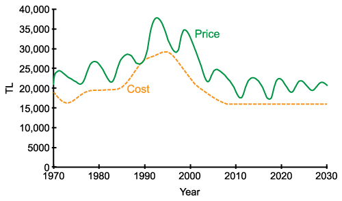
4.29

Figure 8 shows the dynamic behaviors generated by the base model. Price follows the general trend of cost (see Figure 8(a)). Due to the effect of profit margin, the average price is 26% higher than the average cost. The range of the realized profit margin is between 0% and 46%. More importantly, price exhibits oscillations with an average period of 7 years. The main reason behind this oscillation is the negative loop and the delays between demand creation and new house construction. This delay includes the time spent in starting new projects as well as the construction duration. During this period, due to shortage of supply, which can be seen as a decrease in supply/demand ratio in Figure 8(b), price increases. The construction firms do not take into account the constructions in progress and continue to start new projects in order to benefit from the high profits in the market. As the constructions are completed, the demand has already been met, and an excess supply emerges, which causes a decrease in price. The lag between the demand and the supply (new houses) is clearly seen in Figure 8(c).

4.30

As seen in Figure 8(d), effect of profit on the construction start rate is usually close to 1, which means that the companies try to construct new houses as much as excess demand. Sometimes, expected profit falls below normal profit as shown in Figure 8(e). This causes a decrease in effect of profit on construction start rate and the construction companies decide to meet a smaller portion of estimated excess demand.

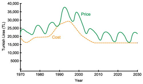
(a) Behaviour of cost (input) and price (output)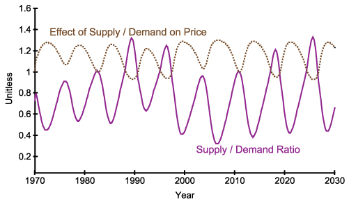

(b) Behaviour of supply/demand ratio and its effect on price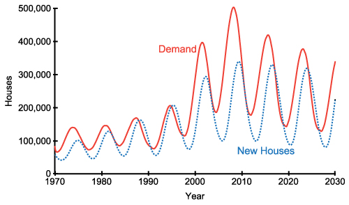

(c) Behaviour of demand and new houses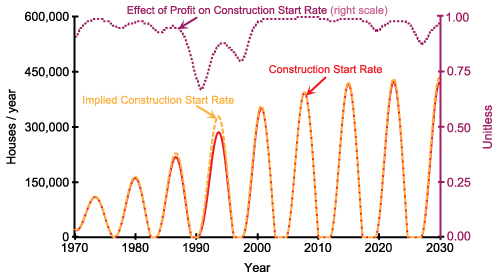

(d) Behaviour of construction start rate and the effect of profit on it. (Implied construction start rate is defined as estimated excess demand divided by construction realization time)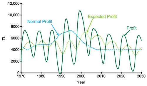

(e) Behaviour of profit-related variables

Figure 8. Behaviors of the base model

Validation

4.31

Since system dynamics models are long-term behavior-oriented descriptive models, their validity cannot be measured by their capabilities of making point forecasts. Rather, they are evaluated in terms of their structural adequacy and their power of generating valid behavior patterns. Validity of the behaviors can be checked against available real behavior patterns, or against logically predicted behaviors under extreme conditions. Thus, there are two main aspects of validation of system dynamics models: structure validity and behavior validity (Barlas 1989, 1996; Saysel & Barlas 2006). Structure validity is assuring that model structure is in agreement with the relations existing in the real life. Behavior validity tests, on the other hand, assess if the model and the real system produce similar output behavior patterns. Validation tests applied in this study are based on the methodology given in Barlas (1996). One should keep in mind that in causal-descriptive modeling, the essence of validity is structure validity: without a valid structure, output behavior validity can be meaningless, entirely coincidental. Behavior validity is useful and meaningful, only after structure validity has been established.

4.32

For the structure validity, we made use of relations from literature that are proven to be consistent with the real system. Our model makes use of many key concepts and structures that are used in the housing economics literature: a chain of stocks representing houses under construction and new houses (Maisel 1963); the dependence of construction start rate on the difference between supply and demand (DiPasquale & Wheaton 1994); gradual price adjustment (DiPasquale & Wheaton 1994); two types of demand creation: due to growth and due to turnover (Barras 2005); demand amplification when price is high (Kenny 1999); and delays in price formation, demand and profit estimation, construction starts and completions (Barras 2005). We also incorporate structures commonly used in system dynamics literature to model similar phenomena: using information delay structures to model adaptive expectations (Sterman 2000); 'effect' formulations to express nonlinear causal relations (Barlas 2002); aging chains to represent consecutive material delays where flows are conserved (Forrester 1970).

4.33

Additionally, the units of the left and right hand sides of all equations are checked and verified that they are consistent. For testing the logical validity of model behavior, we compared the model behavior under extreme conditions with the logically expected behavior in the same conditions. For example, in one of such extreme condition test, we set the initial value of the potential buyers stock and net increase in number of households to zero and showed that the houses under construction are completed but no new houses are constructed (Figure 9(a)) and the price is only affected from changes in the cost as given in Figure 9(b). In another test, we set cost to a constant value, as given in Figure 10. Under this condition, the oscillatory behavior of price still exists which shows that the oscillatory behavior of price is a result of the model's internal structure itself, not a result of the external inputs. This result is particularly important, as it shows that the behavior validity of the model is obtained not by fine-tuned external inputs, but by the internal structure of the model ('right behavior for the right reasons' principle).

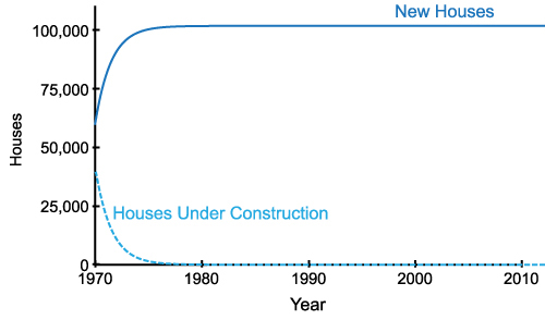
(a) Behaviour of housing variables when there is no demand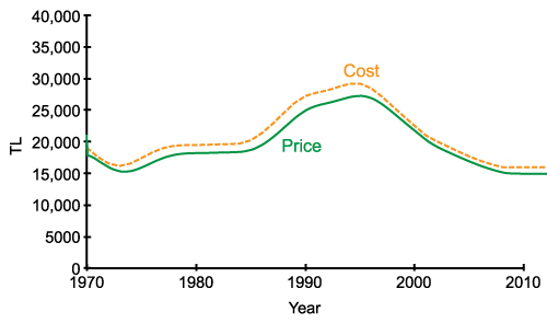

(b) Behaviour of cost and price when there is no demand

Figure 9. Results of the extreme condition validation runs.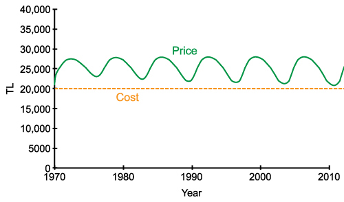

Figure 10. Behavior of price when cost is constant.

4.34

To ensure the behavior validity of the model, the model outputs should be consistent with the real data. It is known that the real estate prices typically show oscillatory behaviors in real life (Figure 1 and Fershtman & Fishman 1992; Meen 2000; Jiang et al. 2010; Genta 1989; Sæther 2008). As Figure 8(a) shows, the behavior of the price variable generated by the model also oscillates similarly. An International Monetary Fund study (Helbling & Terrones 2003) analyzed housing price cycles in 14 developed economies over the 1970 to 2001 period. Over 75 cycles identified, the cycle period is in the range of 0.5–10.5 years with an average of around 4 years. Such rich data for Istanbul real estate market is not available. But as given in Figure 1, the ratio of real estate rent index to the overall price index in Istanbul is available, which can be used for validation purposes. This data series shows oscillations of 6–8 years. The model output for price given in Figure 8(a) shows 7-year price cycles, which is within the range of IMF data and consistent with cycle periods of Istanbul real estate index.

Scenario and Policy Analysis

5.1

In order to prevent the undesired oscillatory behaviors, we need to identify the leverage points that can be used to create changes in the system. This model provides a useful platform for determination of such parameters. Özbaş et al. (2008) performs a sensitivity analysis of an earlier version of the model presented in this paper. The study shows that the amplitude of the price cycles is significantly affected by construction time. As construction time falls, the amplitude of the price cycles also falls. In view of this fact, we conduct a scenario analysis that evaluates the changes in the model when the construction time is decreased.

5.2

Finally we also analyze the effects of a policy that can be applied by the problem owner, which may be a trade chamber, an association or a consortium of real estate construction companies. The policies are evaluated in terms of their effects on the price oscillations.

Decreasing Construction Time

5.3

Our base model assumes that the average construction completion time is about 550 days. Various factors including labor and material shortages, financial difficulties, poor project management, inadequate design and technological limitations cause long delays in construction projects. With the pressure of increasing competition and with the help of technological and managerial strategies, the delays in construction projects can be significantly reduced. The technological strategies may include standardization and repetition of building elements, increasing physical capabilities of machinery, adopting more efficient construction scheduling, or increased use of precast components. The managerial strategies may involve effective site management, providing decision aids, better communication and coordination (Chan & Kumaraswamy 2002).

5.4

This scenario tests what happens if the average construction time is gradually decreased to 150 days linearly in a 10-year period starting from the year 2010. As seen in Figure 11(a), the price cycles damp out and eventually almost disappear. However, complete damping takes about six decades (which cannot be fully observed within the time horizon of the model outputs).

(a) Behaviour of cost (input) and price (output)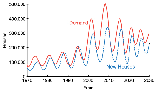

(b) Behaviour of demand and new houses

Figure 11. Behavior of key variables when construction time is decreased by 73% from the year 2010 to 2020.

5.5

The stabilized behavior of price affects the whole system and other variables such as demand, new houses (See 11(b)) and profit gradually approach a steady state after the policy is implemented. This provides a predictable and safe environment for the companies. In a more stable real estate sector, there will be less distortion, lower risk of unemployment and increased output due to reduced mismatch between supply and demand. Less volatile sector creates a much predictable financial environment, which results in lower credit risk assessment.

Companies Take into Account Houses under Construction

5.6

Normally companies do not have enough information about other companies' houses under construction. In this policy, we assume that a central association of companies gathers data on the number of houses under construction, provides the companies with this information and promotes the application of the policy at least by the majority of the companies. Previously, excess demand was computed without taking houses under construction into account as given in Equation 4. In the new policy, the companies use the information about houses under construction in estimating excess demand as shown in Equation 6.

Excess Demand = Potential buyers − New Houses − Houses under construction

(6)

This way, the unnecessary house construction is avoided, which was the main cause of the price oscillations. Figure 12(a) shows behavior of price when this policy is applied after the year 2010. This policy makes the price cycles disappear almost immediately, but the equilibrium price level of this policy is higher than that of the previous scenario.

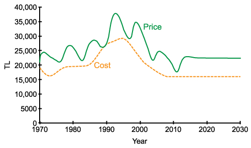
(a) Behaviour of cost (input) and price (output)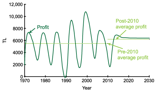

(b) Behaviour of profit

Figure 12. Behavior of key variables when companies start considering houses under construction in their decisions after the year 2010.

5.7

Like price, profit oscillates until new policy is adopted in the year 2010. After the new policy, profit comes to a steady behavior (see Figure 12(b)). When we compare the average yearly profits of pre-policy and post-policy periods, a 13% increase is observed. That is, considering houses under construction in construction decisions makes the market stable and also increases the profits. In a stabilized market the companies will also enjoy the previously mentioned benefits. Finally note that in reality perfect information about houses under construction would not be available to the decision makers. A more realistic version of this ideal scenario can be easily implemented in our model, by incorporating and estimation delay and estimation error in houses under construction in the decision equation. In this case, the oscillatory behaviors would again be stabilized, but not to the extreme extent obtained in the idealized policy (See Figure 13).

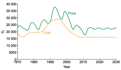
Figure 13. Behavior of cost and price when companies start considering houses under construction with a one-year delay and 10% error after the year 2010.

5.8

Realistic combination of the above two policies; A mild reduction of the construction delays and an imperfect/delayed access to the "number of houses under construction" information would have more real-life relevance. In this case, the oscillatory behavior of the base model is again stabilized (See Figure 14).

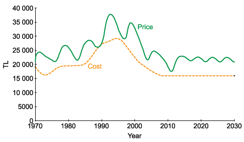
Figure 14. Behavior of cost and price when construction time is decreased by 42% from the year 2010 to 2020, and companies start considering houses under construction with a one-year delay and 10% error after the year 2010.

Conclusion

6.1

The purpose of this study is to model and analyze by simulation the dynamics of endogenously created oscillations in real estate (housing) prices. A system dynamics simulation model is built to understand some of the structural sources of cycles in the key housing market variables, from the perspective of construction companies. The model focuses on the economic balance dynamics between supply and demand. Because of the unavoidable delays in the perception of the real estate market conditions and construction of new buildings, prices and related market variables exhibit strong oscillations. Two policies are tested to reduce the oscillations: decreasing the construction time, and taking into account the houses under construction in starting new projects. Both policies create significantly reduced oscillations, more stable behaviors.

6.2

Real estate markets exhibit cyclic behaviors worldwide. The main reason behind these cycles is the imbalance between the demand and the supply, which is caused by the delays involved in construction decisions and in completing the constructions. Even though construction companies know about the oscillatory behaviors of the market, they try to take autonomous actions to increase their profits in the boom times. Additionally decisions taken during boom and boost times alter the price cycles. In other words, price oscillations are to a large extent produced by the very actions that these companies take. The main paradox is that companies do know about the cycles, but they do not change their main strategies to eliminate them, because they believe that these cycles are exogenously created, not as a result of their very own policies. This paradox is demonstrated by the model and is one of the main motivations behind the study. The resulting complex atmosphere creates a volatile and unstable environment for the companies. In order to create a more stable environment, the companies should act in coordination, since no single company has enough power to control the market.

6.3

We develop a system dynamics simulation model of housing market to understand the causal mechanisms that result in cyclic behavior of the market. The model is built from the perspective of an association of construction of companies in a city, which has enough power to guide the housing market. The structure of the model is generic for developing cities and the parameters are chosen from the city of Istanbul. Three major balancing feedback loops determine the behavior of the model: demand-price, supply-price and supply-demand loops. These balancing feedback loops imply that there is a natural tendency towards stabilization of the system. However, significant delays in these loops result in an oscillatory behavior of the price. Thus, we see that delays are the critical components of this system that can be used as a leverage to reduce undesired oscillations. Based on this observation, we propose alternative policies to reduce the oscillations by decreasing delay durations.

6.4

In one simulation scenario, the construction delays are reduced by technological and managerial strategies. A gradual decrease of construction times by 73% in 10 years eventually causes price cycles to dampen over time. However, the complete elimination of cycles takes place in a 60-year period, beyond the time horizon of the base simulations. Since the full transition takes a long time, the adaptation of the construction companies to the changing environment should not be difficult. On the other hand, the system must be patient enough to enjoy the full benefits of this policy, and 60 years may be too long to be realistic in this sense.

6.5

In an alternative policy, we assume that the construction companies have access to the "number of houses under construction" information when they start new projects. This information can prevent companies building more houses than necessary, which was yielding excess supply and oscillations in the base scenario. With the new policy, the price oscillations are eliminated in a much shorter period of time compared to the first policy. Such a quick change in the market behavior may be hard to adopt, but it results in a 13% increase in the yearly profits when the policy shows its full effect. Realistic combination of the above two policies; A mild reduction of the construction delays and an imperfect/delayed access to the "number of houses under construction" information would have more real-life relevance. In this case, the oscillatory behavior of the base model is moderately stabilized.

6.6

Since the model represents the main causal relationships that are relevant to the housing market cycles, it can also serve as a basis for foreseeing the reaction of the market to other changes in the system. With the help of this model, it will be possible to analyze how sensitive the oscillations are to changes in some parameters such as sales time, construction time and profit margin. Various other policy alternatives can be tested by minor modifications in the model. It is also possible to modify and adapt the model to different specific cities and regions around the world.

Appendix: Model Equations

Construction Realization Time = 0.4 years
Construction Start Rate [houses/yr] = Estimated Excess Demand × Effect of Profit on Construction Start Rate / Construction Realization Time
Houses under Construction(t) [houses] = Houses under Construction(t − dt) + (Construction Start Rate − Construction Rate) × dt
Houses under Construction(1970) = 40000 houses
Construction Time = 1.5 years
Potential Construction Rate [houses/yr] = (Houses under Construction / Construction Time)
Construction Capacity [houses/yr] = GRAPH(t)

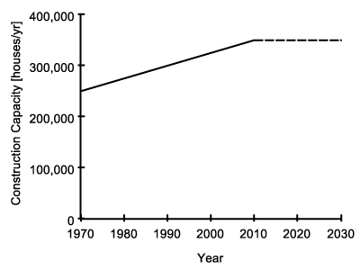
Figure 15. Construction Capacity

Effect of Capacity on Construction Rate [Unitless] = GRAPH(Construction Capacity / Potential Construction Rate)

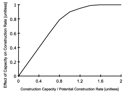
Figure 16. Effect of Capacity on Construction Rate

Construction Rate [houses/yr] = Potential Construction Rate × Effect of Capacity on Construction Rate
New Houses(t) [houses] = New Houses(t − dt) + (Construction Rate − Sales Rate) × dt
New Houses(1970) = 60000 houses
Sales Rate [houses/yr] = MIN(Possible sales, Desired Sales)
Sold Houses(t) [houses] = Sold Houses(t − dt) + (Sales Rate − Demolition Rate) × dt
Sold Houses(1970) = 600000 houses
House Life = 40 years
Demolition Rate [houses/yr] = Sold Houses / House Life
Net Increase in Number of Households [households/yr] = GRAPH(t)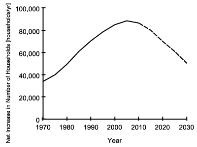

Figure 17. Net Increase in Number of Households

Potential Buyers(t) [households] = Potential Buyers(t−dt) + (Net Increase in Number of Households + Demand Creation Due to Demolition − Demand Satisfaction Rate) × dt
Potential Buyers(1970) = 60000 households
Dwellers(t) [households] = Dwellers(t−dt) + (Demand Satisfaction Rate − Demand Creation Due to Demolition) × dt
Dwellers(1970) = 600000 households
Demand Satisfaction Rate [households/yr] = Sales Rate / Demand per Household
Demand Creation Due to Demolition [households/yr] = Demolition Rate Rate / Demand per Household
Demand [houses] = Potential buyers × Demand per Household × Effect of Price on Demand
Demand per Household = 1 house/household
Cost [TL] = GRAPH(t)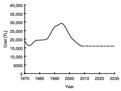

Figure 18. Cost

Perceived Cost(t) [TL] = Perceived Cost(t − dt) + (Perceived Cost Adjustment Rate) × dt
Perceived Cost(1970) = 19100 TL
Perceived Cost Adjustment Time = 0.5 years
Perceived Cost Adjustment Rate [TL/yr] = (Cost − Perceived Cost) / Perceived Cost Adjustment Time
Accepted Profit Margin = 0.1
Indicated price [TL] = Perceived Cost × (1+Accepted Profit Margin)
Price [TL] = Indicated Price × Effect of Supply/Demand on Price
Historical Price(t) [TL] = Historical Price(t − dt) + (Historical Price Adjustment Rate) × dt
Historical Price(1970) = 25000 TL
Historical Price Adjustment Rate [TL/year] = (Price − Historical Price) / Historical Price Adjustment Time
Historical Price Adjustment Time = 5 years
Supply/Demand Ratio [Unitless] = New houses/Demand
Perceived Supply/Demand Ratio (t) [unitless] = Perceived Supply/Demand Ratio (t − dt) + (Perceived Supply/Demand Ratio Adjustment Rate) × dt
Perceived Supply/Demand Ratio Adjustment Rate [Unitless] = (Supply/Demand Ratio − Perceived Supply/Demand Ratio) / Perceived Supply/Demand Ratio Adjustment Time
Perceived Supply/Demand Ratio Adjustment Time = 0.2 years
Effect of Supply/Demand on Price [Unitless] = GRAPH(Perceived Supply/Demand Ratio)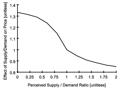

Figure 19. Effect of Supply/Demand on Price

Effect of Price on Demand [Unitless] = GRAPH(Price / Historical Price)

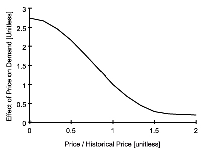
Figure 20. Effect of Price on Demand

Effect of Supply/Demand on Sales Time [Unitless] = GRAPH(1/Perceived Supply Demand Ratio)

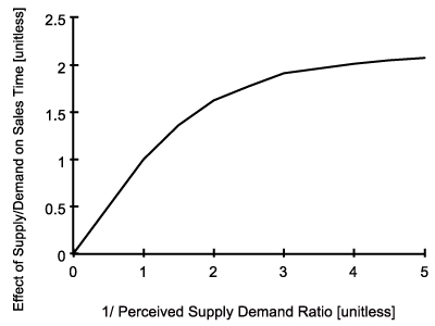
Figure 21. Effect of Supply/Demand on Sales Time

Normal Sales Time = 1 year
Sales Time [years] = Normal Sales Time × Effect of Supply/Demand on Sales Time
Possible sales [houses/yr] = New houses / Sales Time
Desired Sales [houses/yr] = Demand / Sales Time
Profit [TL] = Price − Cost
Expected Profit(t) [TL] = Expected Profit(t − dt) + (Expected Profit Adjustment Rate) × dt
Expected Profit(1970) = 4000 TL
Expected Profit Adjustment Time = 5 years
Expected Profit Adjustment Rate [TL/yr] = (Profit − Expected Profit) / Expected Profit Adjustment Time Profit Margin = 0.25
Normal Profit [TL] = Cost × Profit Margin
Effect of Profit on Construction Start Rate [Unitless] = GRAPH(Expected Profit / Normal Profit)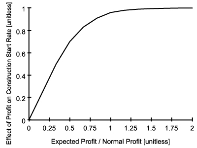

Figure 22. Effect of Profit on Construction Start Rate

Excess Demand [houses] = Potential Buyers − New houses
Estimated Excess Demand(t) [houses] = Estimated Excess Demand(t − dt) + (Excess Demand Adjustment Flow) × dt
Estimated Excess Demand(1970) = 10000 houses
Excess Demand Estimation Time = 1 year
Excess Demand Adjustment Flow [houses/yr] = (Excess Demand − Estimated Excess Demand) / Excess Demand Estimation Time

References

ANAS, A. (1978). Dynamics of urban residential growth. Journal of Urban Economics, 5(1), 66–87. [doi:10.1016/0094-1190(78)90037-2]

ANAS, A., & Arnott, R. J. (1993). Development and testing of the Chicago prototype housing market model. Journal of Housing Research, 4(1), 73–130.

AOKI, K., Proudman, J., & Vlieghe, G. (2004). House prices, consumption, and monetary policy: a financial accelerator approach. Journal of Financial Intermediation, 13(4), 414–435. [doi:10.1016/j.jfi.2004.06.003]

BARLAS, Y. (1989). Multiple tests for validation of system dynamics type of simulation models. European Journal of Operational Research, 42(1), 59–87. [doi:10.1016/0377-2217(89)90059-3]

BARLAS, Y. (1996). Formal aspects of model validity and validation in system dynamics. System Dynamics Review, 12(3), 183–210. [doi:10.1002/(SICI)1099-1727(199623)12:3<183::AID-SDR103>3.0.CO;2-4]

BARLAS, Y. (2002). System dynamics: systemic feedback modeling for policy analysis. In Knowledge for Sustainable Development - An Insight into the Encyclopedia of Life Support Systems, (pp. 1131–1175), Paris, Oxford: UNESCO-EOLSS.

BARRAS, R. (2005). A building cycle model for an imperfect world. Journal of Property Research, 22(2–3), 63–96. [doi:10.1080/09599910500453905]

BINAY, S., & Salman, F. (2008). A critique on Turkish real estate market. Discussion Paper 2008/8. Ankara: Turkish Economics Association.

CHAN, D. W. M., & Kumaraswamy, M. M. (2002). Compressing construction durations: lessons learned from Hong Kong building projects. International Journal of Project Management, 20(1), 23–35. [doi:10.1016/S0263-7863(00)00032-6]

COSKUN, Y. (2011). Housing market in Turkey: an overview. In J. Gimber (Ed.) European Mortgage Federation: Mortgage Info. October 2011.

DELOITTE. (2010). Türkiye gayrimenkul sektörü raporu. Technical Report. Republic of Turkey Prime Ministry Investment Support and Promotion Agency.

DIPASQUALE, D., & Wheaton, W. C. (1994). Housing market dynamics and the future of housing prices. Journal of Urban Economics, 35(1), 1–27. [doi:10.1006/juec.1994.1001]

ESKINAZI, M., Rouwette, E., & Vennix, J. (2011). Houdini: a system dynamics model for housing market reforms. Proceedings of the 29th International Conference of the System Dynamics Society, Washington, DC, USA.

FAIR, R. C. (1972). Disequilibrium in housing models. The Journal of Finance, 27(2), 207–221. [doi:10.1111/j.1540-6261.1972.tb00955.x]

FERSHTMAN, C., & Fishman, A. (1992). Price cycles and booms: dynamic search equilibrium. The American Economic Review, 1221–1233.

FILATOVA, T., Parker, D., & van der Veen, A. (2009). Agent-Based Urban Land Markets: Agent's Pricing Behavior, Land Prices and Urban Land Use Change. Journal of Artificial Societies and Social Simulation, 12(1).

FORRESTER, J. W. (1961). Industrial Dynamics. Cambridge, MA: M.I.T. Press.

FORRESTER, J. W. (1970). Systems analysis as a tool for urban planning. IEEE Transactions on Systems Science and Cybernetics, 6(4), 258-265. [doi:10.1109/TSSC.1970.300299]

GALLIN, J. (2008). The Long-Run Relationship between House Prices and Rents. Real Estate Economics, 36(4), 635–658. [doi:10.1111/j.1540-6229.2008.00225.x]

GENTA, P. J. (1989). Understanding the Boston real estate market: a system dynamics approach. Unpublished Diploma thesis: Massachusetts Institute of Technology.

HARGREAVES, B. (2008). What do rents tell us about house prices? International Journal of Housing Markets and Analysis, 1(1), 7–18. [doi:10.1108/17538270810861120]

HAURIN, D. (1988). The duration of Marketing Time of Residential Housing, AREUEA Journal, 16(5), 396–410. [doi:10.1111/1540-6229.00463]

HELBLING, T., & Terrones, M. (2003). Identifying Asset Price Booms and Busts. World Economic Outlook, April 2003. International Monetary Fund.

HIANG, L. K., & Webb, J. R. (2007). Are international real estate markets integrated: evidence from chaotic dynamics. Technical Report, October 2007. Hartford: Real Estate Research Institute.

HO, Y. F., Wang, H. L., & Liu, C. C. (2010). Dynamics Model of Housing Market Surveillance System for Taichung City. Proceedings of the 28th International Conference of the System Dynamics Society, Seoul, Korea.

HONG-MINH, S., & Strohhecker, J. (2002). A system dynamics model for the UK private house building supply chain. Proceedings of the 20th International Conference of the System Dynamics Society, Palermo, Italy.

ISEE systems. (2009). STELLA. Version 9.1.

JIANG, Y., Feng, L., Dan, M., & Tan, X.-q. (2010). Housing market cycle in China: An empirical study based on stock-flow model. Proceedings of the 2010 International Conference on Management Science & Engineering, Melbourne, Australia.

KENNY, G. (1999). Modelling the demand and supply sides of the housing market: evidence from Ireland. Economic Modelling, 16(3), 389–409. [doi:10.1016/S0264-9993(99)00007-3]

KESKIN, B. (2008). Hedonic analysis of price in the Istanbul housing market. International Journal of Strategic Property Management, 12(2), 125–138. [doi:10.3846/1648-715X.2008.12.125-138]

MU, L., Ma, J., & Chen, L. (2009). A 3-dimensional discrete model of housing price and its inherent complexity analysis. Journal of Systems Science and Complexity, 22(3), 415–421. [doi:10.1007/s11424-009-9174-6]

KUMMEROW, M. (1999). A system dynamics model of cyclical office oversupply. Journal of Real Estate Research, 18(1), 233–256.

MAISEL, S. J. (1963). A theory of fluctuations in residential construction starts. The American Economic Review, 53(3), 359–383.

MEEN, G. (2000). Housing cycles and efficiency. Scottish Journal of Political Economy, 47(2), 114–140. [doi:10.1111/1467-9485.00156]

MURPHY, A. (2010). A dynamic model of housing supply. Working Paper.

ÖZBAŞ, B., Özgün, O., & Barlas, Y. (2008). Sensitivity Analysis of a Real Estate Price Oscillations Model. Proceedings of the 26th International Conference of the System Dynamics Society, Athens, Greece.

POTERBA, J. M. (1984). Tax subsidies to owner-occupied housing: an asset-market approach. The Quarterly Journal of Economics, 99(4), 729. [doi:10.2307/1883123]

SAYSEL, A. K., Barlas, Y. (2006) Model Simplification and Validation with Indirect Structure Validity Tests, System Dynamics Review, 22(3), 241–262. [doi:10.1002/sdr.345]

SÆTHER, J. P. (2008). Fluctuations in Housing Markets, Causes and Consequences. Unpublished Diploma thesis: University of Bergen.

SELIM, H. (2009). Determinants of house prices in Turkey: Hedonic regression versus artificial neural network. Expert Systems with Applications, 36(2), 2843–2852. [doi:10.1016/j.eswa.2008.01.044]

SMITH, L. B. (1969). A model of the Canadian housing and mortgage markets. The Journal of Political Economy, 77(5), 795–816. [doi:10.1086/259563]

STERMAN, J. (2000). Business dynamics: Systems Thinking and Modeling for a Complex World. Irwin-McGraw-Hill.

TU, Y. (2004). The dynamics of the Singapore private housing market. Urban Studies, 41(3), 605. [doi:10.1080/0042098042000178708]

WEIBULL, J. W. (1983). A dynamic model of trade frictions and disequilibrium in the housing market. The Scandinavian Journal of Economics, 373–392. [doi:10.2307/3439598]

WHEATON, W. C. (1999). Real estate "cycles": some fundamentals. Real Estate Economics, 27(2), 209–230. [doi:10.1111/1540-6229.00772]

WYATT, P. (2007). Real estate development. Working Paper. University of Reading, Henley Business School, School of Real Estate and Planning.