Abstract

Questions concerning how one can influence an agent-based model in order to best achieve some specific goal are optimization problems. In many models, the number of possible control inputs is too large to be enumerated by computers; hence methods must be developed in order to find solutions that do not require a search of the entire solution space. Model reduction techniques are introduced and a statistical measure for model similarity is proposed. Heuristic methods can be effective in solving multi-objective optimization problems. A framework for model reduction and heuristic optimization is applied to two representative models, indicating its applicability to a wide range of agent-based models. Results from data analysis, model reduction, and algorithm performance are assessed.

Keywords:

Agent-Based Modeling, Optimization, Statistical Test, Genetic Algorithms, Reduction

Introduction

1.1

Agent-based models (ABMs) are often created in order to simulate real-world systems. In many cases, ABMs act as in silico laboratories wherein questions can be posed and investigated; such questions often arise naturally in the context of the system in question. For example, an ABM of a financial network might be used to determine which policies lead to maximized profit, while an ABM modeling social networks might be studied to determine the most effective means of transmitting information. Questions concerning how one can influence an ABM in order to best achieve some specific goal are optimization problems. In other contexts, optimization may refer to parameters or model design. It is important to reiterate that the meaning of the term in this study is different – it refers to the optimal choice of a sequence of external inputs to a model in order to achieve a particular goal. The stochasticity inherent in many ABMs means that care must be taken when attempting to solve optimization problems. Under fixed initial conditions, data from individual simulation replications often vary. Thus, careful analysis of ABM dynamics is a prerequisite for the development of optimization techniques. In particular, statistical methods must be brought to bear on the interpretation of simulation results.

1.2

In this study, statistical and optimization techniques are presented which can be applied directly to ABMs: translation of the model to an equation-based form is not necessary. There are several advantages to this approach – such techniques can be applied to virtually any ABM, and there is no need for transformation of either the model or the controls. Repeated simulation is used to obtain reliable results, and controls are applied directly to the ABMs. While there may be models for which this approach fails, the sufficiently broad examples provide good evidence that for large classes of ABMs, meaningful results can be obtained by direct analysis and optimization.

1.3

The goal of this paper is to introduce and illustrate a framework for solving optimization problems using agent-based models. In general, the number of possible solutions to an optimization problem is far too large for enumeration. Thus, heuristic methods must be employed to answer such questions. Computational efficiency is a key factor in this process; as such, the use of scaled approximations can be invaluable. As long as a scaled model faithfully maintains the dynamics of the original, it can be used to solve the optimization problem, resulting in a reduction of run time and computational complexity.

1.4

The paper is organized as follows: standards for data analysis are established and a statistical measure for model similarity is proposed. A heuristic technique known as Pareto optimization is proposed as a means for solving optimization problems. The framework is presented via the use of two models acting as representatives of large classes of ABMs, which ought to hold interest for researchers from a wide variety of disciplines. Brief model descriptions are outlined in the text, and detailed model descriptions following the Overview, Design Concepts, and Details (ODD) protocol for agent-based models (Grimm et al. 2006; Grimm et al. 2010) are provided in the appendices. These descriptions ought to provide enough detail that the model (and results) can be reconstructed and verified by independent research.

Related work

1.5

Optimization problems of the type presented here have been studied in models of influenza and epidemics (Kasaie et al. 2010; Yang et al. 2011), cancer treatment (Lollini et al. 1998; Swierniak et al. 2009), and the human immune system (Bernaschi & Castiglione 2001; Rapin et al. 2010), to name a few. Previous studies have investigated the effect of various model features on outcomes – for example, subway travel on the spread of epidemics (Cooley et al. 2011), mobility and location in a molecular model (Klann et al. 2011), molecular components in a cancer model (Wang et al. 2011), and strategies for mitigating influenza outbreaks (Mao 2011) – while not quite posing formal optimization problems. A study on the effect of ABMs in determining malaria elimination strategies (Ferrer et al. 2010) suggests that results from agent-based models are invaluable in the analysis of interventions.

1.6

In other studies, ABMs have been transformed into systems of differential equations (Kim et al. 2008a) and polynomial dynamical systems (Hinkelmann et al. 2011; Veliz-Cuba et al. 2010), among others. The importance of spatial heterogeneity has been examined in specific (Harada et al. 1995) and more general (Happe 2005) cases, and predator-prey ABMs have been analyzed using statistical methods (Wilson et al. 1993; Wilson et al. 1995).

A framework for solving optimization problems

1.7

The framework is summarized in Figure 1; subsequent sections motivate and explain the process in detail.

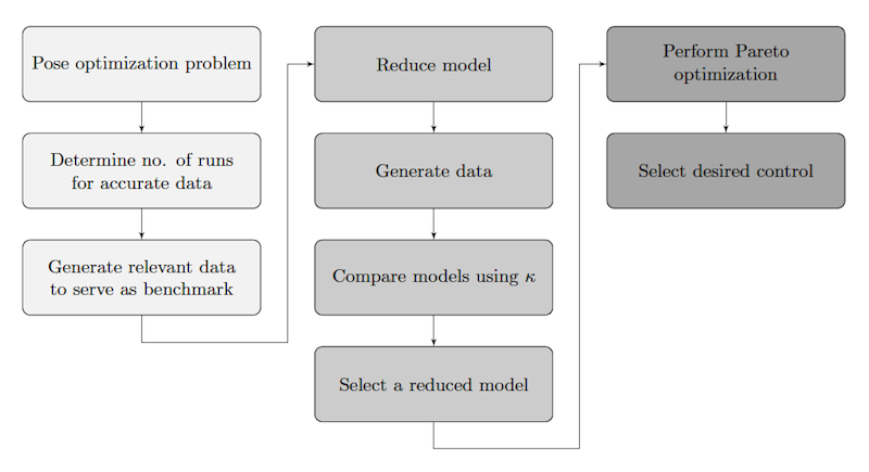
Figure 1. An overview of the framework presented in this work. The three shadings represent the phases of analysis, scaling, and optimization.

Data Reliability

1.8

A key factor in analysis of agent-based models is stochasticity. The approach suggested here is to examine how data averages change as the number of simulations (runs) increases. In many cases, the data will settle in on some average that is not improved upon by increasing the number of runs. Determining a sufficient number of runs is the first step in obtaining reliable results. The emphasis on solving optimization problems necessitates this process: while some of the stochasticity inherent to an individual run is lost when averaging over repeated runs, it is necessary in order to determine the general efficacy of one control versus another.

1.9

Agent-based models are often implemented on a grid, representing the 'space' of the model (often times, the grid indeed represents some physical space). Treating the original size and scope of the model as true, the goal of scaling is to determine the extent to which a model can be reduced without altering pertinent dynamics. The models examined here contain physical agents traversing physical landscapes. In this setting, the strategy is to gradually scale down the model until the dynamics no longer faithfully represent the original model. When applicable, this strategy results in reduced run time – in many cases substantially so – reducing the computational requirements for the solving of optimization problems and allowing access to a wider range of analytical tools.

1.10

Determining to what degree a reduced model is a faithful representation of the original is an important question. In terms of optimization, it is necessary to determine the extent to which models can be reduced for the purpose of optimal control. In order to accomplish this, a sample of the control space is implemented in both the original model and reduced versions. For each reduced version, the controls are ranked according to their effectiveness in regards to the optimization or control objective. The aim is to use a reduced model as a proxy for the original; thus, the ranking of the controls on the reduced model must be compared to the ranking of the same controls applied to the original.

1.11

We propose Cohen's weighted κ (Cohen 1968) as a measure of concordance of rankings for different model sizes. Let p_obs be the observed proportion of agreement in the two lists and let p_exp be the proportion of agreement expected by random chance. Then κ = (p_obs − p_exp)/(1 − p_exp). Hence if the lists are in perfect agreement, κ = 1; if the lists are no more similar than what is expected purely by chance, κ = 0. This similarity metric for ranked lists determines penalties based on the magnitude of disagreement. For details of how to calculate p_obs, p_exp, and weighted penalties, see Cohen (1968).

1.12

For examples of the use of this statistic as a measure of agreement, see Fleiss (1971) and Eugenio (2000). Cohen's weighted κ is chosen because of its wide documentation and implementation in a variety of studies; as such, there is precedent for this measure. There is no objective way to determine a benchmark value for κ. Several studies propose a κ value greater than 0.75 as being very good (Altman 1991; Fleiss 1981), while others recommend a value of 0.8 or higher (Landis & Koch 1977; Krippendorff 1980). In this study no benchmark is set; rather, κ values are assessed a posteriori. For more details on setting a benchmark for κ, see Sim and Wright (2005), and El Emam (1999).

1.13

It is of course not guaranteed that all ABMs will be amenable to the strategies presented here (for discussion on this issue see Durrett and Levin (1994)). In fact, models may exist for which no reduction is possible – nevertheless, reduction strategies are frequently useful and invariably informative. In particular, the investigation of differences in qualitative behavior can be served by these (and other) methods of model reduction. For examples of model reduction strategies applied to ABMs, see Zou et al. (2012), Roos et al. (1991), and Yesilyurt and Patera (1995). It is also worth noting that 'model reduction' is a phrase whose meaning may be discipline-dependent: the extent to which a model can be reduced is dependent on which meaning is taken and which model details one wishes to preserve.

Pareto Optimization

2.1

Once a suitable reduction has been made, an optimization problem can be solved using the reduced model as a surrogate for the original. Perhaps the most explored method for optimal control of ABMs has come in the form of heuristic algorithms. Given that enumeration of the solution space is often infeasible, heuristic algorithms are used to conduct a guided search of the solution space in order to determine locally optimal controls.

2.2

Several heuristic algorithms have been utilized in solving optimization problems for ABMs. Examples include simulated annealing (Pennisi et al. 2008), tabu search (Wang & Zhang 2009), and squeaky wheel optimization (Li et al. 2011). In this study, attention is focused on a certain type of genetic algorithm (GA). These algorithms, first brought to general attention in 1989 (Goldberg 1989), are designed to mimic evolution: solutions that are more fit are used to 'breed' new solutions. GAs have been used in conjunction with ABMs to find optimal vaccination schedules for influenza (Patel et al. 2005), cancer (Lollini et al. 2006), and in determining optimal anti-retroviral schedules for HIV treatment (Castiglione et al. 2007). Vaccination schedule optimization results obtained from simulated annealing and genetic algorithms have even been compared and contrasted (Pappalardo et al. 2010). As the primary focus of this paper is to introduce a general framework for solving optimization problems for ABMs, a comparison of various heuristic methods is outside the scope of this study. For a more comprehensive look at heuristic control of ABMs, see Oremland (2011).

2.3

The control problems described here have multiple objectives – this necessitates assigning weights to each objective. Determination of weights in multi-objective optimization problems can be problematic because a priori, the appropriate weights may be unknown – in particular, the assignment is at the discretion of the investigator. While there have been various proposals for these assignments (for an example, see Gennert and Yuille (1988)), any method which does not require weights has particular appeal.

2.4

Pareto optimization is just such a heuristic method: instead of a focusing on a single solution, the algorithm returns a suite of solutions. Solutions on the Pareto frontier represent those that cannot be improved upon in terms of one objective without some sacrifice in another. In this sense, each solution on the Pareto frontier is optimal with respect to some choice of weights. Thus, the 'managerial' decision of how to assign weights can be settled after the search has concluded.

2.5

An extensive list of references on multi-objective optimization techniques can be found in Coello (2013). Pareto optimization has been selected for this study as it is novel in its application to ABMs. The algorithm adopted here is a minor variant of that described in Horn et al. (1994): it is a heuristic algorithm that searches the control space in an attempt to find the Pareto frontier. Pseudocode for the algorithm is presented in Algorithm 1.

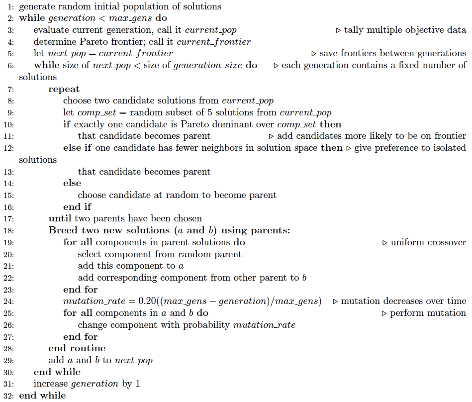
Algorithm 1. Pseudocode for the Pareto optimization algorithm.

Software

3.1

The proposed framework requires two types of software: modeling, and statistical analysis. Agent-based models can be implemented in a variety of software packages. Some of these, such as NetLogo (Wilensky 2009), Repast (North et al. 2006), and MASON (Luke et al. 2005) have been designed for general agent-based modeling. Other software has been developed for agent-based modeling in specific fields – these include C-ImmSim, VaccImm, and SIMMUNE for the human immune system (Castiglione 1995; Woelke et al. 2011; Meier-Schellersheim & Mack 1999), FluTE for influenza epidemiology (Chao et al. 2010), and SnAP for public health studies (Buckeridge et al. 2011). While one can always implement one's own toolkit for examining agent-based models, the use of established software can reduce both the variability between researchers' implementations and the learning curve for conducting research in this field. NetLogo was chosen as the modeling platform in this study, though there is no reason why the study could not have been undertaken using a number of different software packages. A standard NetLogo installation contains an extensive library of models from a variety of fields; the models discussed here are adaptations of popular models from this built-in library. Statistical analysis can be performed by virtually any statistical software package; in this study, Microsoft Excel was used. Due to the fact that simulation data was needed in order to perform Pareto optimization, this process was implemented in NetLogo as well. In general, the techniques described here are sufficiently straightforward that highly specialized software is not needed, and the framework is not limited to any particular software choice.

Two Models

Rabbits and Grass

4.1

The first model to be examined is based on a sample model from the NetLogo library (Wilensky 2009) involving rabbits in a field. At each time step, each rabbit moves, eats grass (if there is grass at its location), and then possibly reproduces or dies, based on its energy level. There are several compelling reasons for the use of this model as a test case for the proposed framework. One is that the model is sufficiently simple to describe, so results can be obtained, interpreted, and understood with minimal overhead. A more important reason is that this model represents the category of general predator-prey systems (with grass functioning as prey). Such models are commonly used in ecology and have been widely studied. Thus, the framework can be presented through an example that appeals to a broad community of researchers. Indeed, this model illustrates many concepts common in ABMs containing interacting species. A detailed description of the model and a list of parameter values are provided in Appendix A.

4.2

Control consists of deciding (each day) whether or not to apply poison to the grid (i.e., uniformly to all grid cells). Specifically, the control objective is to determine a poison schedule u that minimizes the number of rabbits alive throughout the course of a simulation while also minimizing the number of days on which poison is used. Note that it is unlikely that one control schedule will minimize both objectives simultaneously: for example, the control wherein no poison is used certainly minimizes the second objective, but not the first. Thus, this problem is a good candidate for Pareto optimization: a suite of solutions can be found, each member of which is optimal depending on the weights assigned to the two objectives.

Scaling results

4.3

One of the control objectives concerns the average number of rabbits alive over the course of a simulation; thus, this is the pertinent metric in terms of model reduction (given that the other control objective – minimizing days on which control is used – is entirely preserved at any model size and for any number of runs).

4.4

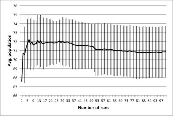
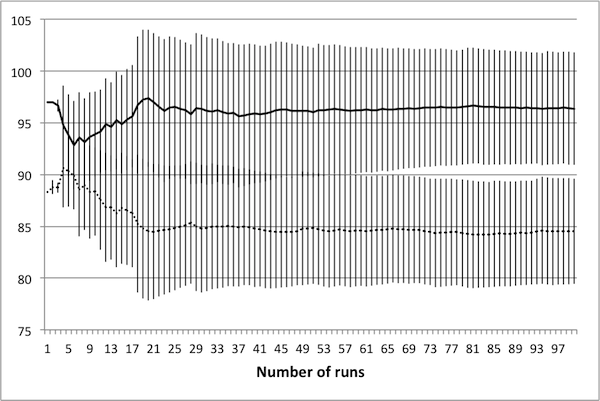
As noted in Data Reliability, the first consideration when attempting to scale the model is determining the number of runs necessary in order to achieve reliable results. To this end, several control schedules were selected at random. Each was applied to the original 50 × 50 model, and results were tallied up to 100 runs. Population dynamics for three randomly selected control schedules are presented in Figure 2: plots show how the average number of rabbits alive over the course of the schedule change as the number of runs increases, with error bars representing one standard deviation.

(a) 10 control days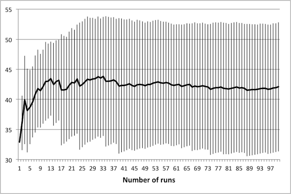

(b) 30 control days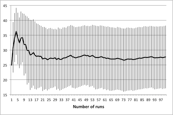

(c) 50 control days

Figure 2. Average population values settle in to consistent values around 50 runs.

4.5

These three schedules represent three distinct regions of the control space, in that each contains a different number of control days. Note that in all cases, there is little change in the mean or the standard deviation beyond 50 runs – this suggests that there is no advantage in averaging over more than 50 runs. It is important to note that if the control objectives were altered (for example, if grass levels were of interest rather than rabbit levels) then this conclusion may not hold. In particular, the necessary number of runs depends upon the model dynamics of interest – in this case, the average number of rabbits.

4.6

Once a benchmark for reliable results has been established, various model reductions can be investigated with respect to control. In the original model, there are 50 × 50 = 2500 patches and 150 rabbits initially. A model size of M means that the world width and height are both M. Hence, when reducing the model to size M, the initial number of rabbits ought to be 150(M²/2500) in order to maintain the same proportion of rabbits to model size. All other state variable values remain the same.

4.7

For each of a set of controls applied to the original model, average rabbit numbers are obtained via simulation; the controls can then be ranked by these numbers. These same controls can be applied to a reduced model, resulting in a (potentially) different ranked list. The κ statistic (see Data Reliability) measures the similarity between the two rankings, thereby serving as a measure of the extent to which the reduced model serves as a substitute for the original. It is important that these rankings are maintained over a wide range of control schedules, since solving the optimal control problem will involve the potential examination of the entire solution space.

4.8

Generating a set of controls randomly results in a normal distribution centered on solutions with fifty zeros and fifty ones (ones indicating time steps on which poison is used). To avoid focusing on too narrow a portion of the control space, a stratified random sample was taken: 24 values N₁, … , N₂₄ were chosen as frequency numbers, representing the number of ones in the schedule. These values were chosen at random within the following scheme: three values were chosen between 1 and 10, three between 10 and 20, and so on, with the final three chosen between 70 and 80. Four control schedules were then randomly generated, each containing N_t ones and (100 − N_t) zeros (distributed randomly throughout the schedule), for t ∈ {1, …, 24}. Thus, for each trial, a total of 96 schedules were evaluated, chosen as representatives of the solution space. Note that schedules with more than 80 non-zero entries were not considered, as preliminary investigation showed that such schedules were quickly eliminated from any heuristic optimal control search.

4.9

One trial is defined as follows: 96 control schedules (chosen according to the above description) were run using the original M = 50 model, and then again on the model at each of the following model sizes: 50, 40, 30, 20, 10, 5, and 3. Note that the schedules are run twice on the original M = 50 model: this is done in order to establish how consistent the rankings are when evaluated twice on the same-sized model. In some sense, this serves as validation of the choice of 50 simulations as being sufficient for reliable results, and also provides insight into the analysis of an appropriate benchmark for κ, as will be seen below.

4.10

Evaluation of 150 schedules (each averaged over 50 simulations) at model size M = 50 requires approximately 3 seconds. Table 1 gives the number of simulations that can be run for the reduced models in approximately 3 seconds. Given that the primary advantage for scaling models is to reduce run time, it is more appropriate to compare data based on equivalent run time rather than using a fixed number of simulations for each size. This data aids in scaling analysis: if one wishes to reduce the run time by 50%, the number of runs that can be performed is easily calculated.

Table 1: Number of simulations in equivalent run time.
World size	Simulations	Avg. run time (sec.)
50	50	3.04
40	75	3.00
30	135	3.05
20	290	3.03
10	1100	3.03
5	3500	3.01
3	5700	3.03

4.11

Figure 3 summarizes κ values for various world sizes and run times. Each data point represents the mean taken over ten trials, with error bars representing one standard deviation. A benchmark value of κ =0.8 is plotted as well – it is presented to serve as a preliminary gauge of how well the reduced models capture the dynamics of the original. Each line on the graph connects data points of equivalent run time. Figure 3 helps identify unviable reductions: accepting a benchmark of κ=0.8, world sizes below 20 are not sufficiently accurate representatives of the original model (and the size 20 model is only sufficient at 100% run time). The data also show that if one insists on using the size 3 model, the benchmark for κ will have to be lowered. It further shows that if one wishes to use the size 3 model and insists on a κ value higher than 0.8, it will certainly require an increase in the run time of the model (and even then, may not be possible).

4.12

Several important conclusions can be drawn from this data: one is that if the priority is achieving the highest possible value for κ, then the original size 50 model is always the best choice for any fixed run time. This is perhaps unsurprising, as one can only expect to lose some accuracy as model size decreases.

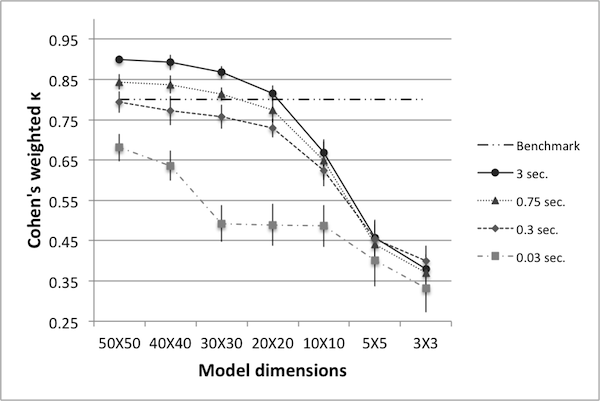
Figure 3. Cohen's weighted k for various world sizes and run times.

4.13

Another important conclusion is that if the only priority is decreased run time, it is always better to use fewer runs of the size 50 model rather than more runs of a smaller model. This follows because each line represents a fixed run time, and for any fixed run time, the size 50 model results in the highest value for κ. A fixed benchmark for κ further informs a researcher with a priority of reduced run time: as the data show, if one wishes to keep κ above 0.8, then it is possible to reduce the run time by 90%, but not further (as indicated by the data for the size 50 model at 0.3 seconds). Thus, not only can one determine which world size should be used in order to obtain minimum run time, but also the minimum run time that can be achieved in order to maintain a pre-set benchmark for κ.

4.14

There may be cases where a reduced model is of particular interest – for example, Hinkelmann et al. (2011) describes methods for translating ABMs into polynomial dynamical systems, offering advantages such as steady state and bifurcation analysis. The number of required equations may be too large for the size 50 model, but not so for the size 10 model. A similar concern applies to differential equations approximations. Examples of these considerations are discussed in Kim et al. (2008a) and Kim et al. (2008b). Hence, depending on the priority of the modeler, the data here show which world sizes may be used and what κ values can be expected when doing so. Furthermore, note that for smaller world sizes the range of κ values is decreased. In particular, in order to achieve 1% run time on the 50 × 50 model, κ decreases from 0.90 to 0.68. However, in order to achieve a 1% run time on the 3 × 3 model, κ decreases from 0.38 to 0.33. Thus, for smaller models κ may be less affected by a decrease in run time.

4.15

In addition to the above conclusions, the data informs the study of points at which the dynamics of the model undergo a qualitative change. There is a larger change in reducing from world size 10 to 5 than there is in going from size 20 to 10; this indicates the dynamics are more rapidly changing between world sizes 10 and 5. In particular, the data seem to suggest that the pertinent dynamics are not drastically altered between the original size 50 model and the size 20 model, but change rather quickly at smaller sizes. This is of particular interest in light of the fact that the original world size was chosen more or less arbitrarily. If one began with a size 10 model, it may not be possible to reduce it to the same extent that one can reduce a size 50 model.

4.16

As mentioned in Data Reliability, several studies suggest a κ value of 0.8 as a benchmark for sufficient similarity. While largely cited and used, the applicability of this value ought to be examined in light of the results obtained by heuristic algorithms. In particular, for each model size an appropriate κ value can be determined a posteriori based on said results. The goal of this model reduction analysis is not to prescribe which model size one 'should' use; rather, given that the process depends on the priority of the modeler, the goal is to present κ values and run times one can expect when using a particular reduced model.

Results from Pareto Optimization

4.17

As discussed in Pareto optimization, the goal of a Pareto optimization algorithm is to return a suite of solutions, each of which is optimal for a particular choice of objective weights. For this model, the objectives are to minimize the number of days on which control is used and to minimize the number of rabbits alive during the course of a simulation. Recall that a control is a vector of length 100 with entries in {0, 1}. Figure 4 shows an example of the Pareto frontier. Each dot corresponds to one control, plotted according to the values on the axes. The ×'s make up the Pareto frontier of this data set: for every point on this frontier, one of the objectives cannot be improved upon without some sacrifice in the other. On the other hand, for each point not on the frontier, there exists some point in the set that improves upon both objectives: in particular, for every square (i.e., non-Pareto frontier) data point, there exists at least one other point with fewer control days and a lower average number of rabbits. The goal of the heuristic Pareto optimization algorithm is to determine, as near as possible, the true Pareto frontier of the control space. Thus, remaining figures consist of Pareto frontiers only and not the entire data sets. In order to investigate a variety of κ values as determined in Scaling results, several representative model sizes and run times were chosen. For each representative model the Pareto optimization algorithm was run and a Pareto frontier obtained. If a reduced model is a suitable substitute for the original then the Pareto frontier for the reduced model ought to be the same as the Pareto frontier of the original model. For each reduced model, the controls making up the frontier are implemented in the original model in order to determine if they are actually Pareto optimal (as the reduced model results has suggested). Note that Pareto optimization has been performed on the original model as well in order to serve as a basis for comparison.

4.18

Figure 5 summarizes results for representative models with lower κ values. Each shape corresponds to one representative model, with results coming from the implementation of these controls in the original model. These results suggest that models with κ values below 0.5 are not very good surrogates for the original model. In particular, there are fewer data points, and they tend to cluster near certain regions of the frontier. In short, very few of the controls determined to be Pareto optimal by these representative models are in fact Pareto optimal in the original model. Figure 6 shows similar results for models with higher κ

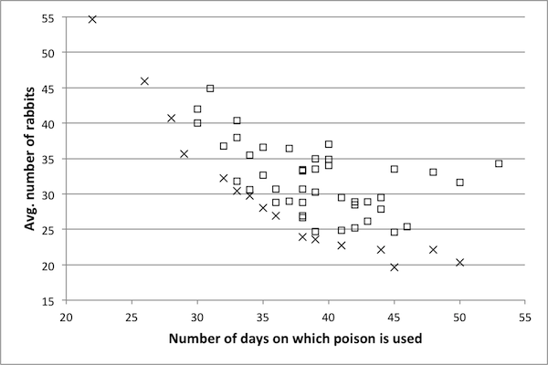
Figure 4. An example Pareto frontier for the Rabbits and Grass model. Frontier points are marked with an x and non-frontier points with a square.

values. The representative model with a κ score of 0.89 produces a Pareto frontier very near to the frontier of the original model, suggesting that a κ value of 0.89 is sufficiently high – hence, a reduced model with a κ value of 0.89 can likely be used as a surrogate for the original model. The data for the model with a κ value of 0.76 is also near to the Pareto frontier of the original model, though not to the same extent. For the model with κ =0.65, there are fewer data points, and these are a bit further from the true frontier.

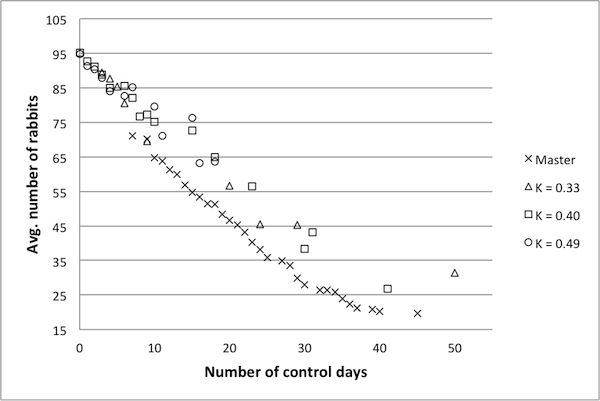
Figure 5. Pareto frontiers for models with lower k values.

4.19

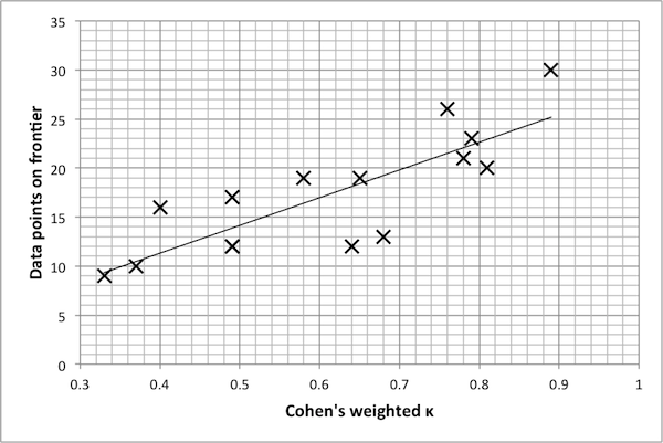
Finally, Figure 7 suggests that there is a mildly linear relationship between the κ value of a reduced model and the number of points on the Pareto frontier. The same settings were used for each Pareto optimization algorithm; yet, in general, this data shows that models with lower κ values tend to produce smaller Pareto frontiers (even within the reduced model itself). One possible explanation for this is that for a reduced model, there is a narrower range in the possible dynamics of a model, and thus the true Pareto frontier for a reduced model may indeed be smaller. Thus, again, κ values indicate the extent to which

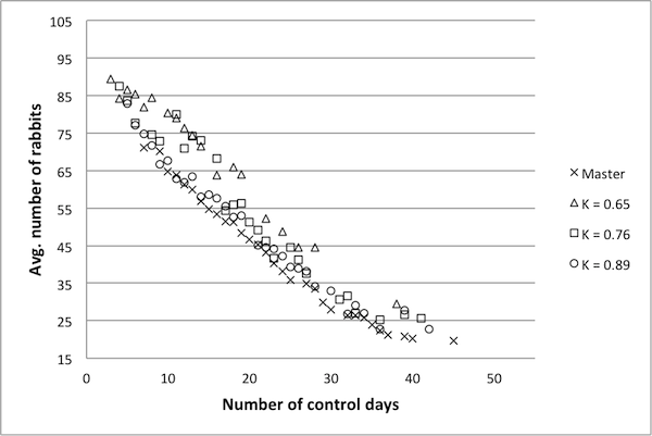
Figure 6. Pareto frontiers for models with higher k values.

model dynamics are preserved. A qualitative examination of the data presented here suggests that a κ benchmark in the region of 0.75 – 0.80 is in fact a good benchmark for this example. Once again, the final decision rests with the researcher and is ultimately determined by the level of desired accuracy.

>

Figure 7. Plot of k value vs. size of frontier, with line of best fit (Pearson's r2 = 0.66).

SugarScape Model

4.20

The second model is a modified version of SugarScape (Epstein 1996), in which a population of agents traverse a landscape in search of sugar. This model was chosen for several reasons: first, it is spatially heterogeneous. This is a common feature of many ABMs and thus it is important to demonstrate how the framework presented here can be applied to models wherein space is an issue. Second, the model has been examined by researchers in a variety of fields – studies based on SugarScape have focused on migration and culture (Dean et al. 2000), distribution of wealth (Rahman et al.2007), and trade (Dasclu et al. 1998). As such, it is of broad general interest as a test case. Thus, future work may build on the framework presented here as a means of conducting research in areas as diverse as social science, biology, and economics.

4.21

The basis of the model used here is included with the standard NetLogo distribution (Wilensky 2009). The landscape consists of fixed regions containing different amounts of sugar; as such, this model contains a spatial heterogeneity not present in the rabbits and grass model. The original landscape is presented in Figure 8; darker regions represent areas with more sugar. Periodically, ants are taxed based on their vision, metabolism, and location (e.g., high-vision ants in sugar-rich regions may be taxed at higher rates than low-vision ants in regions with less sugar). The optimization problem is to determine the tax schedule that maximizes the total tax income collected while minimizing the number of deaths. Full model details, including those pertaining to taxation, are provided in Appendix B. Note that certain parameter values are altered when considering reduced models; parameter values in Appendix B refer to the 50 × 50 model.

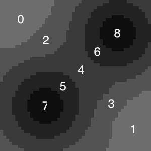
Figure 8. Landscape of the 50x50 SugarScape model. Darker regions contain more sugar. Each region is labeled with a number; Table 8 provides maximum sugar levels by region.

Scaling Results

4.22

A total of 100 controls were generated, consisting of three different average tax rates. The number of deaths and tax income for each was collected over a total of 100 runs. Representative data is presented in Figure 9, with error bars representing one standard deviation. As seen in the figure, there is very little change in the mean and standard deviation of the data beyond 50 runs; hence, there is no benefit to averaging over more than 50 simulations.

4.23

Given the importance of the spatial layout of the SugarScape model, it is necessary to preserve this layout as nearly as possible in any reduced version. Landscape reduction was determined by the nearest-neighbor algorithm, a means of re-sampling the original landscape in order to determine the layout of a reduced version.

4.24

In addition to scaling the map, the number of agents was also scaled. While low vision is defined to be 1 at any model size, high vision depends on the size of the grid: an agent with vision v on a 50 × 50 grid has vision v_n = v(n / 50) on an n × n grid. For grid sizes 10 and 5, this would result in high vision being equivalent to low; thus in these two cases high vision was defined to be 2. The metabolism of each agent is not scaled: at each model size, it was randomly set between 1 and 4 (inclusive).

4.25

To run the simulation 50 times at model size M = 50 (meaning a 50 × 50 grid) takes approximately 8.5 seconds. Table 2 shows the number of simulations that can be run in equivalent run time for reduced model sizes.

(a) Avg. tax rate of 0.125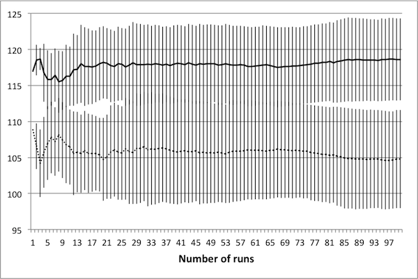

(b) Avg. tax rate of 0.25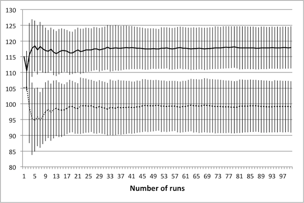

(c) Avg. tax rate of 0.375

Figure 9. Average values for deaths (solid) and tax income (dashed) again settle in to consistent values by 50 runs. Tax income values have been scaled linearly to fit on the plots.

4.26

Figure 10 shows κ values for various model reductions. Since there are two variables in this case (deaths and tax income), controls can be ranked according to either, resulting in two different κ values. Note that when ranked according to the number of deaths, κ values are extremely low – in fact, close to being completely random. While the rankings according to tax income result in higher κ values, they still fall short of the proposed minimum benchmark of 0.8.

Table 2: Number of simulations in equivalent run time.
World size	Simulations	Avg. run time (sec.)
50	50	8.51
40	88	8.48
30	173	8.49
20	427	8.52
10	1375	8.53
5	3900	8.48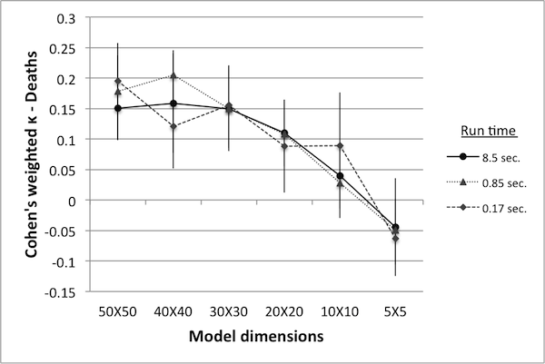

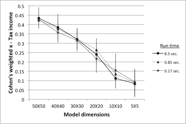
Figure 10. Cohen's weighted k with controls ranked by deaths (left) and by tax income (right).

4.27

An interesting feature of this data is that there appears to be no great difference in the κ values obtained from models run at 2% of the original run time versus those obtained from 100% run time. This may indicate that the number of runs used for reliable data was originally set too high, or it may indicate that κ values at or below 0.45 are equally unreliable. Nevertheless, there is a clear trend showing that as the model size decreases the κ values decrease as well. As in the previous example, this may be an indication of qualitative changes in model dynamics as the model size is reduced.

Results from Pareto Optimization

4.28

Although κ values appear lower in this case, it is necessary to again examine the performance of reduced models with respect to control. While the suggested benchmark of 0.75 – 0.8 proved fitting for the previous model, it may be that a lower κ benchmark is acceptable in this case. Results are presented in Figure 11.

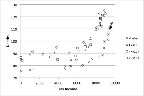
Figure 11. Pareto optimization results for SugarScape.

4.29

Pareto frontiers from three models are presented here: those with κ values of 0.43, 0.27, and 0.15 (with respect to tax income). The shapes of the data from the three models follow the same basic shape of the true Pareto frontier (labeled 'Master' in the figure), but there is a distinct difference in performance. In particular, none of the controls found by any of these models are on the Pareto frontier of the original. Furthermore, there does not appear to be any significant difference between solutions found using the model with κ =0.43 and those found using the model with κ =0.15. This indicates that not only are none of these models appropriate as replacements for the original, but that there may in fact be a minimum κ value, below which all models are unsuitable. In other words, the downward trend indicated in Figure 10 may be misleading: while it seems to suggest that as model size decreases, the models become less representative of the dynamics of the original, the results in Figure 11 suggest that this isn't actually the case. On the contrary, models with a κ value of 0.15 may be no worse than those with κ values of 0.43. Given that no models attained a κ value higher than 0.45, it is impossible to judge the benchmark of 0.75 as appropriately high. On the other hand, it is possible to conclude that κ values at or below 0.45 are certainly too low.

Conclusions

5.1

The goal of this paper is to introduce a framework for optimization of agent-based models. Once reliable data is obtained, reduced models can be compared to the original. Similarity can be measured using Cohen's weighted κ. Pareto optimization was implemented in order to solve control problems in both cases, allowing for a posteriori analysis of the κ benchmark. Results presented here show that in one example, the established benchmark in the range of 0.75 – 0.8 was indeed sufficient for model reduction, while the second example showed that values below 0.45 were too low. These results suggest κ can be a meaningful measure for model reduction.

5.2

The models presented here were selected for their universality and popularity – as such, they act as standard models to which any attempt at analysis should be applied. In principle there is no reason why the methodology would not apply to extensions of these models or to other ABMs. In the future this collection of models should be expanded to include a wider variety of models of increasing complexity. This methodology has been applied here to models wherein space and agent location are key features; it may require some modification in order to generalize to non-spatial models. In addition, other methods for analysis of agent-based models include transformation to equation models. Such work (using the same models presented here) is underway.

5.3

As ABMs are used more and more to investigate real-world systems, optimization and optimal control problems will naturally arise in the context of ABMs. Heuristic methods have several advantages: they are easy to implement on a computer and they can be applied to virtually any ABM. This is particularly important for models that are too complex for conversion to other mathematical forms, e.g., in cases where differential equations are insufficient. The user has direct control over how each algorithm runs, and can fine-tune parameters and settings to better suit the model. However, there are drawbacks to these methods. For those interested in the certainty of finding globally optimal solutions, heuristic methods are lacking. On the other hand, one may obtain sufficient controls using these methods, and that is a step in the right direction for control of ABMs – in particular when one's goal is to obtain controls that are either sufficient or simply better than any previously known.

5.4

It is possible that the complexity of agent-based models will make formulaic translation to rigorous mathematical models intractable – in that case, heuristic methods provide the only means for optimization and optimal control of agent-based models. Coupled with the model reduction techniques and analysis introduced here, this technique provides valuable methodology for solving control problems with agent-based models.

Acknowledgements

Funding for this work was provided through U.S. Army Research Office Grant Nr. W911NF-09-1-0538, and some ideas were developed by the Optimal Control for Agent-Based Models Working Group at NIMBioS, University of Tennessee. Additionally, the authors are grateful to reviewers for their careful consideration of the manuscript. Many helpful suggestions were implemented due to reviewer feedback.

Appendices

A: Overview, Design concepts, and Details (ODD) protocol for Rabbits and Grass

The model upon which this version is based is included in the sample library of NetLogo (Wilensky 2009), a popular agent-based modeling platform. The description here is warranted as it includes the mechanics of an optimization problem, the details of which are not available elsewhere.

Purpose

The purpose of this model is to examine population dynamics of a simple environmental system. In particular, it is a model of rabbits eating grass in a field. On each day of the simulation, poison can be placed on the field in order to kill the rabbits. This version of the model is an attempt to answer the following optimization question: what is the best way of controlling (i.e., minimizing) the rabbit population while also minimizing the amount of poison used?

Entities, state variables, and scales

This section contains a description of the grid cells, spatial and temporal scales, and the rabbits. It also contains a description of the format of a poison schedule, the investigation of which is the key feature of the model.

Grid cells, spatial scale, and temporal scale. The world is a square grid of discrete cells, representing a field. The grid is toroidal: edges wrap around both in the horizontal and vertical directions. The distance from the center of a cell to a neighboring horizontal or vertical cell is 1 unit (thus the distance between two diagonal cells is sqrt(2)). Units are abstract spatial measurements. Time steps are also abstract discrete units. A simulation consists of a finite number of time steps. The only state variable for each cell indicates whether or not the cell currently contains grass. When grass is eaten on a grid cell there is a certain probability that it will grow back at each time step. This growth happens spontaneously.

Table 3: Grid cell state variables.
State variable	Name	Value
Side length of field	s	50 grid cells
Total grid cells	N	2500
Presence of grass	grass?	0 = no grass, 1 = grass
Grass growth probability	γ/0.02
Simulation time	total_sim_time	100 time steps

Rabbits. Each time step, rabbits move, eat grass (or not), and reproduce (or not). Reproduction is asexual and based on energy level, which is raised when a rabbit eats. Rabbits lose energy both by moving and by spawning new rabbits. If a rabbit's energy level drops to 0 or lower the rabbit dies.

Table 4: Rabbit state variables.
State variable	Name	Value
Movement cost	move_cost	0.5
Energy from food	food_energy	3
Birth threshold	birth_threshold	8
Current energy level	energy	varies

Poison schedule. A poison schedule u is a vector of length total_sim_time with each entry either 0 or 1. Each entry corresponds to one time step in the simulation; 0 means that poison is not used and 1 means that poison is used. Thus, there are a total of 2^( total_sim_time) possible poison schedules. The poison has a maximum efficacy that degrades over time with repeated use. If the poison is not used the efficacy increases again, up to the maximum.

Table 5: Poison schedule details.
State variable	Name	Value
Maximum efficacy	p_max	0.3
Degradation rate	p_deg	5
Current efficacy	p_eff	Varies in (0, p_max]

Process overview and scheduling

In order to minimize ambiguity, details of model execution are presented as pseudocode; see Algorithm 2.

Design concepts

In the updated ODD protocol description (Grimm et al. 2010) there are eleven design concepts. Those that do not apply have been omitted.

Basic principles. In essence, this model is a predator-prey system wherein the rabbits are predators and the grass is prey. Introduction of poison into the model, and having that poison modeled as a direct external influence on population levels, creates a natural setting for an optimization problem. One can study the effect of various poison strategies on population levels – in terms of minimizing the rabbit population it can be thought of as a harvesting problem, but in terms of minimizing poison it can be thought of as resource allocation.

Algorithm 2. Pseudocode for the Rabbits and Grass process and scheduling.

Emergence. Rabbit population and grass levels tend to oscillate as the simulation progresses. The frequency and amplitude of these oscillations can be affected by parameter settings and initial values and hence may be described as emergent model dynamics.

Interaction. Agent interaction is indirect: since rabbit movement is executed serially, it is possible that other rabbits deplete all of the grass in a particular rabbit's potential field of movement, thereby reducing or eliminating the chance for that rabbit to gain energy.

Stochasticity. Rabbit movement is totally random in that they cannot sense whether neighboring grid cells contain grass or not. Whether grass grows back on an empty grid cell is also random, and a grid cell that has been empty for several time steps is no more likely to grow grass than a cell that has only just become empty.

Observation. Rabbit population and grass counts are recorded at each time step. The total number of rabbits alive during the course of a simulation serves as a measure of fitness of the poison schedule.

Initialization

At initialization, 20% of the grid cells contain grass; these are chosen at random. There are 150 rabbits placed at random locations throughout the grid. Each begins with a random amount of energy between 0 and 9 inclusive (rabbits with 0 energy may survive the first time step by eating grass). Total simulation time is 100 time steps and each simulation contains a poison schedule u, described in Poison schedule.

Input data

There is no input data to the model.

Submodels

The model contains no submodels.

Optimization

Since the multi-objective optimization problem is the key feature of the model as presented here, a few clarifying details are in order. The objectives of the optimization problem are to determine, for the parameter values provided, a set of Pareto optimal poison schedules that minimize the number of rabbits while also minimizing the amount of poison used. The number of rabbits refers to the total number of rabbits alive during the course of a simulation – not just those alive at the end of the final time step. Since a poison schedule is a binary vector of length total_sim_time, the amount of poison used is represented by the sum of the entries of that vector.

B: Overview, Design concepts, and Details protocol for SugarScape with taxation

Purpose

The version of SugarScape presented here is a modified version of the original SugarScape (Epstein 1996), a model in which abstract entities roam a landscape made of sugar. These agents are periodically taxed for their sugar stores – the tax rate is constant but the frequency differs from region to region. The purpose of this version of SugarScape is to investigate the effects of various taxation policies on tax income and agent population. In particular, the model is used to investigate the following question: what is the optimal taxation policy for maximizing collected income while minimizing deaths?

Entities, state variables, and scales

Ants. Each ant has a fixed vision and metabolism level for the duration of the simulation; these levels vary from ant to ant. Ants can see in the four principal directions up, down, left, and right, but cannot see any other grid cells. Metabolism determines how much sugar an ant loses ('burns') each time step. Movement is governed by vision: an ant moves to the nearest grid cell within its vision with the maximum amount of sugar. Only one ant may occupy a grid cell at any given time. Ants die if their sugar level reaches zero. There is no upper limit to how much sugar an ant may accumulate. Low vision is defined as 1, 2, or 3 and low metabolism is defined as 1 or 2. Thus, each ant belongs to one of the following four categories: low vision / low metabolism (LL), low vision / high metabolism (LH), high vision / low metabolism (HL), and high vision / high metabolism (HH).

Table 6: Ant state variables.
State variable	Name	Value
Location (current region)	reg	{0, 1, … , 8}
Vision	vis	random in {1, 2, … , 5}
Metabolism	met	random in {1, 2, 3, 4}
Sugar	sug	varies in {1, 2, … }

Grid cells. When ants consume the sugar from a grid cell, the sugar grows back at a fixed rate over subsequent time steps, up to a pre-determined maximum based on the layout of the landscape.

Table 7: Grid cell state variables.
State variable	Name	Value
Maximum sugar	s_max	one of {0, 1, 2, 3, 4}
Sugar	s_here	{0, 1, 2, 3, 4}
Grow back rate	α/1

Spatial and temporal scales. The landscape for SugarScape is presented in Figure 8. The maximum sugar amounts for each region are given in Table 8. There are five region types: those whose maximum sugar is 0, 1, 2, 3, or 4. Each ant occupies exactly one grid cell, and the map is toroidal – edges wrap in both the horizontal and vertical directions. The landscape is a 50 × 50 grid of cells. Given the fairly abstract nature of the model, time and space are unitless. A simulation consists of a finite number of time steps.

Table 8: Maximum sugar and grid cell counts for each region.
Region	0	1	2	3	4	5	6	7	8
Max. sugar	0	0	1	1	2	3	3	4	4

Taxes are collected at regular intervals. The tax rate for a given ant depends on its category and current region (for example, an agent with high vision and low metabolism may be taxed at rate 0.75 in a high-sugar region but only at 0.25 in a low-sugar region). Tax amounts are always rounded up to the nearest integer – this ensures that any non-zero tax rate always collects at least 1 unit of sugar. Taxes are collected once every subsequent 5 time steps for a total of ten tax cycles. The choice to tax every 5 ticks is motivated by the desire to not let the dynamics stabilize – with frequent taxation the dynamics are more immediately affected by previous tax rates.

Table 9: Taxation and temporal variables.
Variable	Name	Value	Units
Simulation duration	total_sim_time	50	time steps
Permissible tax rates	tax	{0, 0.25, 0.5, 0.75}	N/A
Tax interval	tax_interval	5	time steps

For each of the four ant categories there are five possible tax rates depending on their current region and each of these rates may be different for each of the ten tax cycles. Thus, a tax schedule is a vector of length 5 · 4 · 10 = 200 with each entry in {0, 0.25, 0.5, 0.75} – this means there are a total of 4^(200) different tax schedules. The optimization problem is to determine the tax schedules that maximize the total tax income collected while minimizing the number of deaths.

Process overview and scheduling

The ABM process is presented in Algorithm 3 as pseudocode. The ant and tax routines are executed fully by one ant, then fully by another – i.e., serially. Hence state variables are updated asynchronously. Time steps are discrete units, as is movement: ants jump directly from the center of one grid cell to the center of another.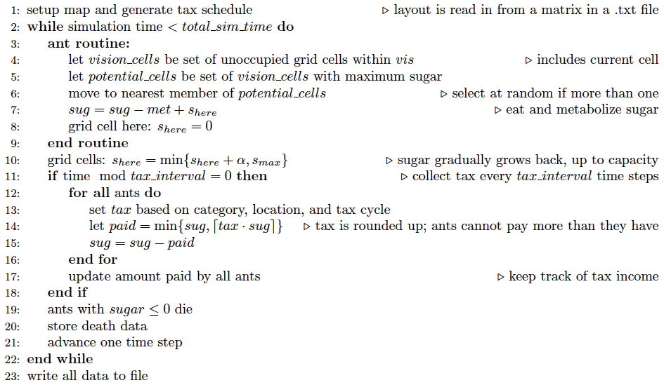

Algorithm 3. Pseudocode for SugarScape process and scheduling.

Design concepts

Basic principles. This version of SugarScape builds on the original by incorporating taxation. In general, the basic question under investigation is how spatially-dependent local inputs affect global dynamics. Specifically, the model investigates how local tax rates affect tax income and regional population distribution, a question which holds interest in a variety of real-world settings.

Emergence. Spatial population dynamics ought to be an emergent property of the model: for example, high tax rates in high-sugar regions might substantially alter regional population dynamics. The precise mechanism driving such changes is not built in to the model in any direct sense.

Objectives. The objective of each ant is to move to a cell within its vision with the maximum amount of sugar. There is no other consideration, and ants do not have knowledge of past or future tax rates at any location.

Sensing. Ants are aware of the sugar level and occupancy of each grid cell within their vision. They are not aware of any properties of any other ants, even those within their vision.

Interaction. Ants interact with one another indirectly in the sense that only one ant may occupy a grid cell at any given time. Thus if two ants have the same high-sugar grid cell within their vision, whichever ant is randomly selected to move first will occupy that cell. This may very well alter the movement of the other ant. In this way, serial execution and asynchronous update are key features of agent interaction. If ant order was not random (i.e., the same ant was allowed to move first each time step), population dynamics might be fundamentally altered.

Stochasticity. Ant movement is partially stochastic: if an ant sees four unoccupied grid cells with 2 sugar and three unoccupied grid cells with 3 sugar, the ant will choose the nearest cell with 3 sugar. This 'minimum distance' policy tends to lead to ants clustering on regional boundaries, as they have limited incentive to move to the interior of a region. This movement feature is discussed in Epstein and Axtell (1996).

Collectives. In a sense, ants form collectives that affect individuals inside and outside of the collective. This arises because only one ant may occupy a grid cell at any time. In high-sugar regions, ants in the middle of the region tend to become trapped because all available spaces are occupied. At the same time, an individual on the border of such a region is frequently unable to enter due to the high population density within the region. These collectives form entirely as a result of local interactions.

Observation. Each simulation consists of a finite number of time steps. At each time step, the following information is collected: the total amount of tax collected, and the number of deaths that occur. For each simulation, the tax policy is recorded as well. At the end of each simulation these data are written to a comma separated value (.csv) file, a universal format for spreadsheet applications.

Initialization

The model is initialized with 200 ants; each is placed at a random unoccupied location on the landscape. Ants begin with a random amount of sugar between 5 and 25 (inclusive); this value is different for each ant and chosen from a uniform distribution. Ants are initialized with vision chosen at random between 1 and 5 (inclusive) and metabolism between 1 and 4 (inclusive). Vision and metabolism of a given ant do not change over the course of a simulation.

Input data

The landscape is read in from a .txt file; this helps with implementation and makes it easier to make changes. A tax policy can either be chosen directly via code manipulation or chosen at random. The policy must be chosen prior to simulation. As such, the tax policy may be thought of as input to the model.

Submodels

There are no submodels for this version of SugarScape.

References

ALTMAN, D. (1991). Practical Statistics for Medical Research. London: Chapman and Hall.

BERNASCHI, M. & Castiglione, F. (2001). Design and implementation of an immune system simulator. Comput. Biol. Med. 31, 303–331. [doi:10.1016/S0010-4825(01)00011-7]

BUCKERIDGE, D. L., Jauvin, C., Okhmatovskaia, A. & Verma, A. D. (2011). Simulation Analysis Platform (SnAP): a Tool for Evaluation of Public Health Surveillance and Disease Control Strategies. AMIA Annu Symp Proc 2011, 161–170.

CASTIGLIONE, F. (1995). C-ImmSim Simulator. Institute for Computing Applications, National Research Council (CNR) of Italy. <http://www.iac.cnr.it/~filippo/C-ImmSim.html>.

CASTIGLIONE, F., Pappalardo, F., Bernaschi, M. & Motta, S. (2007). Optimization of HAART with genetic algorithms and agent-based models of HIV infection. Bioinformatics 23(24), 3350–3355. [doi:10.1093/bioinformatics/btm408]

CHAO, D. L., Halloran, M. E., Obenchain, V. J. & Longini, I. M. (2010). FluTE, a publicly available stochastic influenza epidemic simulation model. PLoS Comput. Biol. 6, e1000656. [doi:10.1371/journal.pcbi.1000656]

COELLO, C. (2013). List of references on evolutionary multiobjective optimization. http://www.lania.mx/ ~ccoello/EMOO/EMOObib.html. Archived at: <http://www.webcitation.org/6HhFo4K5H>.

COHEN, J. (1968). Weighted kappa: nominal scale agreement with provision for scaled disagreement or partial credit. Psychol Bull 70(4), 213–220. [doi:10.1037/h0026256]

COOLEY, P., Brown, S., Cajka, J., Chasteen, B., Ganapathi, L., Grefenstette, J., Hollingsworth, C. R., Lee, B. Y., Levine, B., Wheaton, W. D. & Wagener, D. K. (2011). The role of subway travel in an influenza epidemic: a New York City simulation. J Urban Health 88, 982–995. [doi:10.1007/s11524-011-9603-4]

DASCLU, M., Franti, E. & Stefan, G. (1998). Modeling production with artificial societies: the emergence of social structure. In: Cellular Automata: Research Towards Industry (Bandini, S., Serra, R. & Liverani, F., eds.). Springer London, pp. 218–229.

DEAN, J. S., Gumerman, G. J., Epstein, J. M., Axtell, R. L., Swedlund, A. C., Parker, M. T. & McCarroll, S. (2000). Understanding Anasazi culture change through agent-based modeling. Dynamics in human and primate societies. Oxford University Press, Oxford , 179–206.

DURRETT, R. & Levin, S. (1994). The importance of being discrete (and spatial). Theoretical Population Biology 46(3), 363–394. [doi:10.1006/tpbi.1994.1032]

EL EMAM, K. (1999). Benchmarking kappa: interrater agreement in software process assessments. Empirical Software Engineering 4(2), 113–133. [doi:10.1023/A:1009820201126]

EPSTEIN, J. M. & Axtell, R. (1996). Growing artificial societies: social science from the bottom up. Washington, DC, USA: The Brookings Institution.

EUGENIO, B. D. (2000). On the usage of kappa to evaluate agreement on coding tasks. In: In Proceedings of the Second International Conference on Language Resources and Evaluation.

FERRER, J., Prats, C., Lopez, D., Valls, J. & Gargallo, D. (2010). Contribution of individual-based models in malaria elimination strategy design. Malaria Journal 9(Suppl 2), P9. [doi:10.1186/1475-2875-9-S2-P9]

FLEISS, J. (1981). Statistical Methods for Rates and Proportions. Hoboken, NJ: John Wiley And Sons.

FLEISS, J. L. (1971). Measuring nominal scale agreement among many raters. Psychological Bulletin 76(5), 378–382. [doi:10.1037/h0031619]

GENNERT, M. A. & Yuille, A. (1988). Determining the optimal weights in multiple objective function optimization. In: Computer Vision, Second International Conference on. [doi:10.1109/ccv.1988.589974]

GOLDBERG, D. (1989). Genetic algorithms in search, optimization, and machine learning. Reading, MA: Addison-Wesley.

GRIMM, V., Berger, U., Bastiansen, F., Eliassen, S., Ginot, V., Giske, J., Goss-Custard, J., Grand, T., Heinz, S. K., Huse, G., Huth, A., Jepsen, J. U., Jrgensen, C., Mooij, W. M., Mller, B., Pe'er, G., Piou, C., Railsback, S. F., Robbins, A. M., Robbins, M. M., Rossmanith, E., Rger, N., Strand, E., Souissi, S., Stillman, R. A., Vab, R., Visser, U. & DeAngelis, D. L. (2006). A standard protocol for describing individual-based and agent-based models. Ecological Modelling 198(1–2), 115–126. [doi:10.1016/j.ecolmodel.2006.04.023]

GRIMM, V., Berger, U., DeAngelis, D. L., Polhill, J. G., Giske, J. & Railsback, S. F. (2010). The ODD protocol: A review and first update. Ecological Modelling 221(23), 2760–2768. [doi:10.1016/j.ecolmodel.2010.08.019]

HAPPE, K. (2005). Agent-based modelling and sensitivity analysis by experimental design and metamodelling: An application to modelling regional structural change. 2005 International Congress, August 23-27, 2005, Copenhagen, Denmark 24464, European Association of Agricultural Economists.

HARADA, Y., Ezoe, H., Iwasa, Y., Matsuda, H. & Sato, K. (1995). Population persistence and spatially limited social interaction. Theoretical Population Biology 48(1), 65–91. [doi:10.1006/tpbi.1995.1022]

HINKELMANN, F., Murrugarra, D., Jarrah, A. & Laubenbacher, R. (2011). A mathematical framework for agent based models of complex biological networks. Bull Math Biol 73(7), 1583–1602. [doi:10.1007/s11538-010-9582-8]

HORN, J., Nafpliotis, N. & Goldberg, D. (1994). A niched pareto genetic algorithm for multiobjective optimization. In: Evolutionary Computation, 1994. IEEE World Congress on Computational Intelligence. Proceedings of the First IEEE Conference on Computational Intelligence [doi:10.1109/icec.1994.350037]

KASAIE, P., Kelton, W., Vaghefi, A. & Naini, S. (2010). Toward optimal resource-allocation for control of epidemics: An agent-based-simulation approach. In: Winter Simulation Conference (WSC), Proceedings of the 2010.

KIM, P. S., Lee, P. P. & Levy, D. (2008a). A PDE model for imatinib-treated chronic myelogenous leukemia. Bull. Math. Biol. 70, 1994–2016. [doi:10.1007/s11538-008-9336-z]

KIM, P. S., Lee, P. P. & Levy, D. (2008b). Modeling imatinib-treated chronic myelogenous leukemia: reducing the complexity of agent-based models. Bull. Math. Biol. 70, 728–744. [doi:10.1007/s11538-007-9276-z]

KLANN, M. T., Lapin, A. & Reuss, M. (2011). Agent-based simulation of reactions in the crowded and structured intracellular environment: Influence of mobility and location of the reactants. BMC Syst Biol 5, 71. [doi:10.1186/1752-0509-5-71]

KRIPPENDORFF, K. (1980). Content Analysis: an Introduction to its Methodology. Beverly Hills, CA: Sage Publications.

LANDIS, J. R. & Koch, G. G. (1977). The measurement of observer agreement for categorical data. Biometrics 33(1), 159–174. [doi:10.2307/2529310]

LI, J., Parkes, A. J. & Burke, E. K. (2011). Evolutionary squeaky wheel optimization: A new analysis framework. Evolutionary Computation. <http://www.mitpressjournals.org/doi/abs/10.1162/EVCO_a_00033>. [doi:10.1162/EVCO_a_00033]

LOLLINI, P., Castiglione, F. & Motta, S. (1998). Modelling and simulation of cancer immunoprevention vaccine. Int J Cancer 77, 937–941. [doi:10.1002/(SICI)1097-0215(19980911)77:6<937::AID-IJC24>3.0.CO;2-X]

LOLLINI, P. L., Motta, S. & Pappalardo, F. (2006). Discovery of cancer vaccination protocols with a genetic algorithm driving an agent based simulator. BMC Bioinformatics 7, 352. [doi:10.1186/1471-2105-7-352]

LUKE, S., Cioffi-Revilla, C., Panait, L., Sullivan, K. & Balan, G. (2005). MASON: A multi-agent simulation environment. Simulation: Transactions of the society for Modeling and Simulation International 82(7), 517–527. [doi:10.1177/0037549705058073]

MAO, L. (2011). Agent-based simulation for weekend-extension strategies to mitigate influenza outbreaks. BMC Public Health 11, 522. [doi:10.1186/1471-2458-11-522]

MEIER-SCHELLERSHEIM, M. & Mack, G. (1999). Simmune, a tool for simulating and analyzing immune system behavior. CoRR cs.MA/9903017.

NORTH, M. J., Collier, N. T. & Vos, J. R. (2006). Experiences creating three implementations of the repast agent modeling toolkit. ACM Trans. Model. Comput. Simul. 16(1), 1–25. [doi:10.1145/1122012.1122013]

OREMLAND, M. (2011). Optimization and Optimal Control of Agent-Based Models. Master's thesis, Virginia Polytechnic Institute and State University.

PAPPALARDO, F., Pennisi, M., Castiglione, F. & Motta, S. (2010). Vaccine protocols optimization: in silico experiences. Biotechnol. Adv. 28, 82–93. [doi:10.1016/j.biotechadv.2009.10.001]

PATEL, R., Longini, I. M., Jr. & Halloran, M. E. (2005). Finding optimal vaccination strategies for pandemic influenza using genetic algorithms. J. Theoret. Biol. 234(2), 201–212. [doi:10.1016/j.jtbi.2004.11.032]

PENNISI, M., Catanuto, R., Pappalardo, F. & Motta, S. (2008). Optimal vaccination schedules using simulated annealing. Bioinformatics 24, 1740–1742. [doi:10.1093/bioinformatics/btn260]

RAHMAN, A., Setayeshi, S. & Shamsaei, M. (2007). An analysis to wealth distribution based on sugarscape model in an artificial society. International Journal of Engineering 20(3), 211–224.

RAPIN, N., Lund, O., Bernaschi, M. & Castiglione, F. (2010). Computational immunology meets bioinformatics: the use of prediction tools for molecular binding in the simulation of the immune system. PLoS ONE 5, e9862. [doi:10.1371/journal.pone.0009862]

ROOS, A. M. D., Mccauley, E. & Wilson, W. G. (1991). Mobility versus density-limited predator– prey dynamics on different spatial scales. Proceedings: Biological Sciences 246(1316), pp. 117–122. [doi:10.1098/rspb.1991.0132]

SIM, J. & Wright, C. C. (2005). The kappa statistic in reliability studies: use, interpretation, and sample size requirements. Phys Ther 85(3), 257–268.

SWIERNIAK, A., Kimmel, M. & Smieja, J. (2009). Mathematical modeling as a tool for planning anticancer therapy. Eur. J. Pharmacol. 625(1-3), 108–121. [doi:10.1016/j.ejphar.2009.08.041]

VELIZ-CUBA, A., Jarrah, A. S. & Laubenbacher, R. (2010). Polynomial algebra of discrete models in systems biology. Bioinformatics 26(13), 1637–1643. [doi:10.1093/bioinformatics/btq240]

WANG, T. & Zhang, X. (2009). 3D protein structure prediction with genetic tabu search algorithm in off-lattice AB model. In: Proceedings of the 2009 Second International Symposium on Knowledge Acquisition and Modeling -Volume 01, KAM '09. Washington, DC, USA: IEEE Computer Society. [doi:10.1109/KAM.2009.2]

WANG, Z., Bordas, V. & Deisboeck, T. (2011). Identification of Critical Molecular Components in a Multiscale Cancer Model Based on the Integration of Monte Carlo, Resampling, and ANOVA. Frontiers in Physiology 2(0). [doi:10.3389/fphys.2011.00035]

WILENSKY, U. (2009). Netlogo. Center for Connected Learning and Computer-Based Modeling, Northwestern University, Evanston, IL. http://ccl.northwestern.edu/netlogo/.

WILSON, W., Deroos, A. & Mccauley, E. (1993). Spatial instabilities within the diffusive lotka-volterra system: Individual-based simulation results. Theoretical Population Biology 43(1), 91–127. [doi:10.1006/tpbi.1993.1005]

WILSON, W., McCauley, E. & Roos, A. (1995). Effect of dimensionality on lotka-volterra predator-prey dynamics: Individual based simulation results. Bulletin of Mathematical Biology 57, 507–526. [doi:10.1007/BF02460780]

WOELKE, A. L., von Eichborn, J., Murgueitio, M. S., Worth, C. L., Castiglione, F. & Preissner, R. (2011). Development of immune-specific interaction potentials and their application in the multiagent-system VaccImm. PLoS ONE 6, e23257. [doi:10.1371/journal.pone.0023257]

YANG, Y., Atkinson, P. M. & Ettema, D. (2011). Analysis of CDC social control measures using an agent-based simulation of an influenza epidemic in a city. BMC Infect. Dis. 11, 199. [doi:10.1186/1471-2334-11-199]

YESILYURT, S. & Patera, A. T. (1995). Surrogates for numerical simulations; optimization of eddy-promoter heat exchangers. Computer Methods in Applied Mechanics and Engineering 121(14), 231–257. [doi:10.1016/0045-7825(94)00684-F]

ZOU, Y., Fonoberov, V. A., Fonoberova, M., Mezic, I. & Kevrekidis, I. G. (2012). Model reduction for agent-based social simulation: coarse-graining a civil violence model. Phys Rev E Stat Nonlin Soft Matter Phys 85(6 Pt 2), 066106. [doi:10.1103/PhysRevE.85.066106]