Abstract

We provide simple general-purpose rules for agents to buy inputs, sell outputs and set production rates. The agents proceed by trial and error using PID controllers to adapt to past mistakes. These rules are computationally inexpensive, use little memory and have zero-knowledge of the outside world. We place these zero-knowledge agents in a monopolist and a competitive market where they achieve outcomes similar to what standard economic theory predicts.

Keywords:

Methodology, Microeconomics

Introduction

1.1

Agents are coordinated by the prices they set. Markets clear when prices balance correctly all possible economic information. Yet individual agents need to set these prices with only some of that information. We present a model where agents endogenously discover and set market-clearing prices using none of that information.

1.2

We give agents simple decision rules that allow them, with no knowledge of demand, supply or market structure, to solve for both competitive and monopolist prices and quantity. We explain how agents trade in section 3 and 4. We then expand them to make the agents also produce and maximize profits in section 5 and 6.

1.3

Agents using these rules are pure tinkerers. They adapt not by learning the real model of the world but by assuming such model is unknowable and then proceeding by trial and error. Tinkering keeps these rules general-purpose.

1.4

We believe this methodology useful for two reasons. First, we provide a ready-made set of decision rules that can be used in almost any other agent-based model. There is no market structure or auctioneer feeding the prices to the agent. We believe them perfect as a baseline to compare to more nuanced decision rules.

1.5

Second, we provide a "rationality floor": the minimum information and rationality needed for markets to work, like the Zero-Intelligence project (Gode & Sunder 1993). Unlike Zero-Intelligence, our rules apply to both trading and production and do not depend on the very strict statistical assumptions that doomed Zero-Intelligence (Cliff et al. 1997).

1.6

The lack of knowledge assumed in this model is extreme to the point of caricature. This is by design. Firstly because the fewer informational assumptions we make, the easier it is to plug-in these rules in other models. Secondly because we can test the robustness of traditional partial equilibrium analysis to a complete violation of standard rationality assumptions.

1.7

As Mäki (2008), but see also Nowak et al. (2011), we claim that the fundamental contribution of any model is to isolate causal mechanisms in a complicated world. Here the mechanism allows firms to maximize profits and price goods correctly just by monitoring the difference between what they produce and what they sell.

1.8

In a more realistic model, firms would have more information and intelligence but they would need to solve a higher dimensional problem trying to manage not just production and prices but also customer satisfaction, labor relations, geography, social networks and so on, mixing all causal mechanisms in a single incomprehensible cacophony of parameters. That model would resemble reality better but it wouldn't be more useful.

Literature Review

2.1

We can categorize market processes along two dimensions: whether the price vector is provided exogenously or discovered endogenously and whether the process allows trades to occur in disequilibrium before the equilibrium price is found.

2.2

Exogenous-equilibrium: the modeler solves for the market clearing prices and assumes they are known to the agents. This requires agents to be as rational, informed and computationally capable as the modeler who created them. Unfortunately the computational ability assumed is very high: even when equilibrium prices are known to exist, the utility is linear and the goods are indivisible, approximating equilibrium prices is NP-hard (Deng et al. 2002). More generally exchange equilibrium is a PPAD-complete problem (Papadimitriou 1994).

2.3

Exogenous-disequilibrium: the modeler imposes a market formula that changes prices in reaction to some aggregate variables like excess demand or productivity. Scarf (1960) is instructive in both explaining the idea and giving examples where an equilibrium exist but this methodology fails to find it. When finding an equilibrium is not an explicit goal, agent-based models use this methodology: for example the wage-setting algorithm in Dosi et al. (2010).

2.4

Endogenous-equilibrium: the agents play a game against one another (for example a Bertrand competition) and choose the Nash equilibrium price and quantity. This still requires agents both to have enough information about their competitors to feed into their best response function and high computational ability: finding Nash-equilibria is also PPAD-complete (Chen & Deng 2006).

2.5

Endogenous-disequilibrium: agents interact and trade between themselves without waiting or solving for equilibrium. The oldest market process model, the Walras's tatonnement, involved independent agents exchanging tickets at disequilibrium prices (see chapter 3 of Currie & Steedman 1990). Agents traded tickets rather than goods because trading goods at disequilibrium creates wealth effects and path dependencies that invalidate welfare theorems; see Jaffe (1967) for a discussion about Walras, see Foley (2010) for a modern treatment on welfare theorems under disequilibrium.

2.6

Modern disequilibrium models usually don't assume welfare theorems hold. We catalog these models by the market structure used. In a strictly bilateral market, agents are randomly matched and barter with one another. There is no single market price but many trade prices. The pricing strategy depends on the matching and bartering functions used. If agents can compare their profitability with the rest of the population, like in Gintis (2007), the prices offered by each agent can be driven by evolutionary methods. If an agent only knows the characteristic of whom it is matched to, like in Axtell (2005), market clears by letting every beneficial barter occur between all trader pairs. Results can be driven by matching rather than bartering, as in Howitt and Clower (2000), where fixed-price shops are built endogenously and agents have to search for the right shops to exchange goods.

2.7

A more general market structure is continuous double auctions with multiple buyers and sellers. Our model belongs to this category. Here the two main behavior algorithms are: Zero Intelligence Plus (Cliff et al. 1997) and the Gjerstad and Dickhaut method (Gjerstad & Dickhaut 1998). They represent the two opposite views on adaptation: tinkering and learning. Zero Intelligence Plus traders tinker with their markup according to the previous auction results while Gjerstad and Dickhaut auctioneers first learn a probabilistic profit function and then maximize it.

2.8

Our algorithm is simpler. Like Zero Intelligence Plus, we set prices by tinkering over previous errors. Unlike Zero Intelligence Plus, we use no auction-specific information and so our algorithm is market-structure independent. Moreover our algorithm can be expanded to direct production and maximize profits rather than just trade. The tinkering and adjustment is simulated through the use of Proportional Integrative Derivative (PID) controllers.

2.9

While control theory is a staple of macroeconomics and PID controllers the simplest and commonest of controls, to the best of our knowledge we are the first to use PID control in economics. The closest paper to our approach is Ortega and Lin (2004) where a PID controller is suggested for inventory control, equalizing new buy orders to warehouse depletion. That is not an economic model as it doesn't deal with prices or markets.

2.10

In the spirit of Bagnall and Toft (2006), we judge our algorithm by testing it in a series of markets where the economic theory identifies a clear optimum.

Zero Knowledge Sellers

3.1

An agent is tasked to sell 100 units of a good every day. It has no information on demand or competition and no opportunity to learn. All the agent can do is set a sale price and wait. If at the end of the day it has sold too much, it will raise the price tomorrow. If it has sold too little, it will lower the price.

3.2

This is an elementary control problem. The seller has a daily target of 100 sales and wants to attract exactly 100 customers a day. The seller has no power over customers themselves and so it needs to manipulate another variable (sale price) to affect the number of customers attracted. The seller doesn't know what the relationship between sale price and customers attracted is and so proceeds by trial and error. The trial and error algorithm used by sellers in this paper is a simple PID controller.

3.3

Given target y* (target sales) and process variable y (today's number of customers), the daily error is:

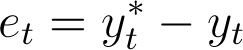
Define u_t as the policy (sale price). The seller manipulates the policy in order to reduce the error. The true relationship between policy and error is unknown, so the seller follows the general rule: "increase the policy when the error is positive, decrease it when the error is negative", which is the definition of negative-feedback control (Åström & Hägglund 2006).

3.4

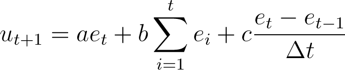
The PID controller manipulates the policy as follows:

Intuitively the policy is a function of the current error (proportional), the sum of all observed errors (integral) and the change from earlier errors (derivative). In discrete time models (as the simulations in this paper) the equivalent formula is:

There are four reasons as to why PID controllers are a good choice to simulate agents' trial and error.

3.5

First, PID controllers assume no available information. Agents using PID rules act only on the outcome of previous choices.

3.6

Second, PID controllers assume no knowledge on how the world works. The PID formula contains no hint on how policy affects the error: there are no demand or supply functions. The PID formula leads agents to tinker and adapt without ever knowing or learning the "true" model.

3.7

Third, PID controllers make no assumptions on what the target should be. The target in the PID formula is completely exogenous. The controllers work regardless of how the target is chosen or how often it is changed.

3.8

Finally, PID controllers can complement other rules through feed-forwarding. Feed-forwarding refers to using PID controllers on the residuals of other rules. For example, take a more nuanced seller choosing its sale price by estimating a market demand function from data. This estimation would provide an approximate prediction of demand given the sale price. Still we could improve this approximation by adding a PID controller to adjust the sale price by setting as error the discrepancy between predicted and actual demand.

3.9

For PID controllers to work, four assumptions need to be made on the market in which they are employed. First, PIDs work by trial and error so the market structure must allow agents to experiment. This means that policies (prices) must be flexible. The stickier the policies, the slower the agent is at zeroing the error.

3.10

Second, PID controllers work better when even small changes in policy have some effects on the error. For zero-knowledge sellers the equivalent assumption is facing a continuous demand function. This does not mean that discontinuities automatically invalidate PID control and in fact all the computational examples in this paper have discrete and discontinuous demands. But PID performance degrades with discontinuities resulting in more overshooting and slower approach to the equilibrium prices.

3.11

Thirdly, PID controllers implicitly assume a downward sloping demand: lower prices increase sales, higher prices decrease them. Zero-Knowledge sellers would fail to price Giffen goods.

3.12

Finally, targets must be achievable. For example, finding the price to sell to exactly n agents in a world with infinitely elastic demand is impossible. The target "exactly n sales" is unreachable: the error will oscillate between n and infinity, never reaching zero. Section 5.2 deals with how to set targets endogenously.

Zero Knowledge Sellers Examples

Mathematical Example

4.1

It is possible to show the workings of a zero-knowledge seller without software. Take a seller facing the unknown demand curve q = 100 − 5p and tasked to sell 5 units of good every day. This zero knowledge seller uses a PID controller with the parameters 0.01 for the proportional error, 0.15 for the integral and 0 for the derivative. The following table tracks the trial and error process of the seller as it discovers the right price (19) and sells the right number of goods..

Table 1:
Day	et		Price (ut)	Quantity to Sell(yt*)	Customers Attracted ()
1	-	-	0	5	100
2	95	95	15.2	5	24
3	19	114	17.290	5	13.550
4	8.55	122.55	18.468	5	7.660
5	2.660	125.210	18.808	5	5.960
6	0.960	126.170	18.935	5	5.325
7	0.325	126.494	18.977	5	5.113
8	0.113	126.607	18.992	5	5.039
9	0.039	126.646	18.997	5	5.005

A Computational Example^[1]

4.2

A seller receives daily 4 units of a good to sell. There is a fixed daily demand made up of 10 buyers. The first is willing to pay $90 or less for one good, the second $80 and so on. The demand repeats itself every day. Agents trade over an order book: the seller sets its price and all crossing quotes are cleared (while supplies last). The trading price is always the one set by the seller. Prices can only be natural numbers.

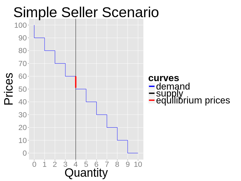
Figure 1. The example's daily market demand and supply

4.3

The seller starts by charging a random price and then adjusts it daily through its PID. The seller target is to sell all its inventory. Unsold goods accumulate. The seller knows only how many customers it attracted at the end of the day. There is no competition.

4.4

With this setup, any price between $51 and $60 (both included) will sell the 4 goods to the 4 top-paying customers. The next figures show the market closing prices of two sample runs. In both cases the seller selects the "right" price: $51.

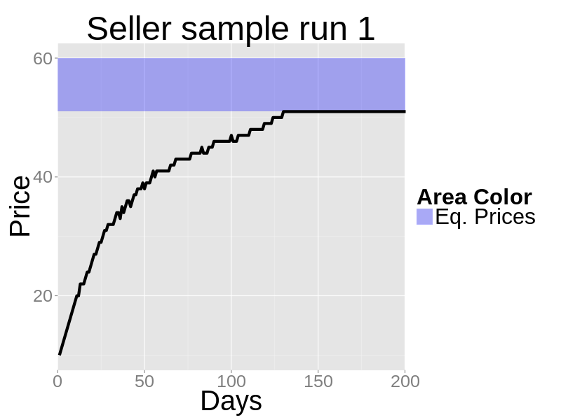
Figure 2. The closing prices of a zero-knowledge seller sample run when the initial random price is below the equilibrium

4.5

Notice how, when the initial price is too high (as in the second run), the adjustment initially undershoots. Undershooting is caused by the firm trying to dispose leftover inventory from previous days; that is, while undershooting, the firm is trying to sell its usual 4 daily goods plus what has not been sold before.

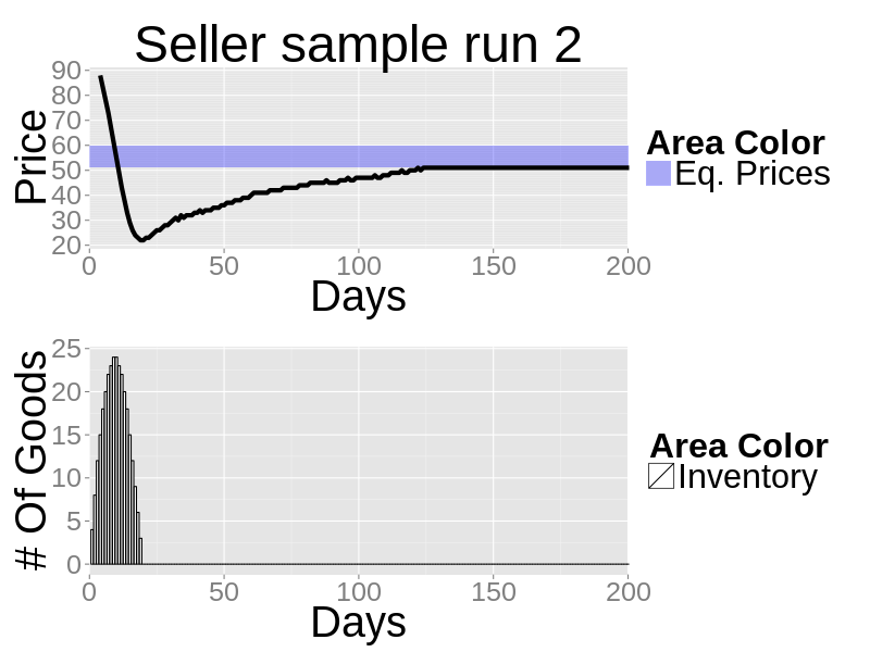
Figure 3. The closing prices and inventory of a zero-knowledge seller sample run when the initial random price is above the equilibrium

PID Parameter Sweep

4.6

The PID equation depends on three parameters. Parameter a for the proportional error, b for the integrative error and c for the derivative one. In the previous example the parameters were a=0.25, b=0.25 and c=.0001. Here we vary the parameters in turn to show their effects on sellers' behavior.

4.7

In the next figure the a parameter varies. An increase in a makes the PID more responsive to today's error. This results in a more jagged price curve, but not a faster approach to the true prices.

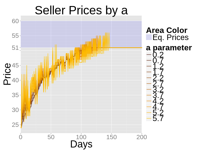
Figure 4. The effects of varying the a parameter of a zero-knowledge seller

4.8

In the next figure the b parameter varies. An increase in b makes the PID more responsive to the cumulative sum of errors. This results in a faster approach to the true prices but it can cause fluctuation and overshooting.

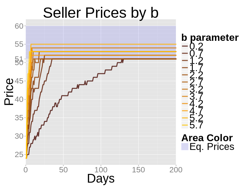
Figure 5. The effects of varying the b parameter of a zero-knowledge seller

4.9

Changing the c parameter (even increasing it by 100 times) has almost no effect in his model. The derivative part of the PID becomes important to smooth overshooting which isn't a real issue to zero-knowledge sellers because their baseline parameters are very small.

A Computational Example with Demand Shifts

4.10

Agents using PID controllers adapt rather than learn. This keeps them working when market conditions change. Here we replicate the zero-knowledge computational example of the previous sections but after 500 days 10 more buyers enter the market. These buyers have a higher demand: the first willing to pay $190, the second $180 and so on. The "right" price, after the shock, moves from $51 to $151.

4.11

The next figure shows the sale prices of a zero-knowledge seller. The seller quickly finds the new price. Notice here that nothing was changed in the seller algorithm. The PID was not told that the demand had shifted. There is no "structural break" detection. Simply the PID reacts to a changing y (number of customers) by increasing prices to hit the old target.

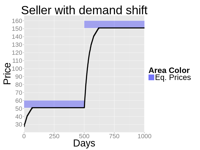
Figure 6. The sale prices of a zero-knowledge seller dealing with a demand shock after 500 days

Zero Knowledge Firms

5.1

A firm is tasked to maximize its profits by producing and selling its output daily. It has no information on customer demand, labor supply or competition. The firm only knows its own production function. The firm has to decide daily and concurrently the sale price of its goods, the wage of its workers and its production quotas. The problem faced by the firm is harder for two reasons: firstly, it has to trade in multiple markets at the same time and secondly, it is a producer, not a passive receiver of endowment.

5.2

Zero-Knowledge firms maximize their profits by dividing the problem into sub-components and solving each separately. There are two equivalent ways to understand this division: by variables or by time.

5.3

Dividing the profit maximization problem by variables means recognizing that the firm has two kinds of variables to set:

• Targets: how much to produce, how much input to buy, how much output to sell, how many workers to hire
• Policies: how much to offer for inputs, how much to ask for outputs, what wages to offer.

Rather than setting them all together at once, we proceed in turn. We manipulate policies in order to achieve targets, and we set targets in order to maximize the profit function.

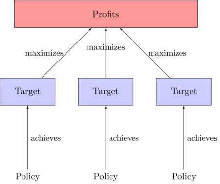
Figure 7. The decision-making problem of the firm split by variables

5.4

The process of profit maximization of the Firm then is split in two classes of operations:

• Control: change policies to achieve targets
• Maximization: change targets to achieve the objective.

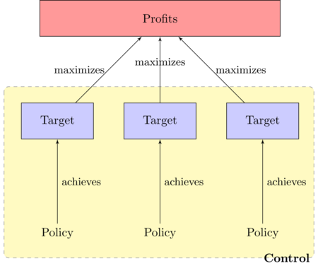
Figure 8. Define control as the process of changing policies to achieve targets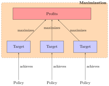

Figure 9. Define maximization as the process of setting target to maximize profits

5.5

The alternative and equivalent way to subdivide the profit maximization process is by focusing on time. Here we take Hicks's (Leijonhufvud 1984) division of time in economics between long run (both capital and labor are variable), short run (labor is variable) and market days (production is fixed and unchangeable). Control is the process of managing Hicksian market days: buying, hiring and selling assuming production can't be changed. Maximization is the process of managing the short run: changing production rate to maximize profits.

5.6

The two processes integrate as a feedback loop. The maximization process sets production targets for the controls. The controls, given time, discover the price associated with those targets. The maximization then uses the discovered prices to adjust to new targets and the loop restarts. This is a trial and error alternative to proper backward induction. Backward induction requires the firm to try every possible target, discover the prices associated with each and then choose the target that maximizes profits. Backward induction is exhaustive learning, while the maximization used by the zero-knowledge firm is just tinkering.

5.7

An example of how the two processes relate in time is the next figure. Control happens every day while maximization occurs less frequently to give control time to discover the right prices. In this example the firm revises its production every 3 days. This frequency is arbitrary, and in fact when and how one temporal phase ends and another begins has always been a weakness of Hicks's temporal model (Currie & Steedman 1990). We will show in the Section 5.2 how to avoid this arbitrariness and link the frequency of maximization with the results from the control process.

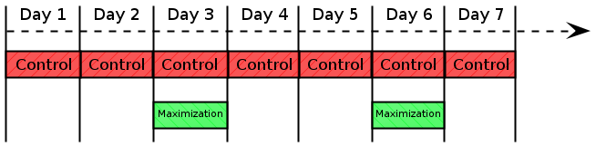
Figure 10. An example of how control and maximization processes occur over time. In this case a firm arbitrarily revise its production quota every 3 days, hence maximization on day 3 and 6. The firm needs to buy inputs and sell output every day, hence control every day of the week

Control

5.8

Control is the process of manipulating policies to achieve targets. In secton 3 we used a PID controller to solve a univariate problem: manipulate one policy to achieve one target. The zero-knowledge firm problem is multivariate.

5.9

We solve this multivariate control problem by splitting it into multiple independent univariate control problems. The zero-knowledge firm is composed of many zero-knowledge traders each achieving a single target with their own PID controller. We call each of these traders a firm's department. This structure is appropriate for object-oriented programming through simple object composition (see the following UML diagram).

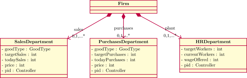
Figure 11. UML Diagram of a generic firm

5.10

We showed how the PID controller solves the seller problem. The following table expands the PID methodology to buying and hiring.

Table 2:
Component	Variable y	Target y*	Policy ut
Purchases	# of goods purchased	# of input needed	Price offered
Sales	# of customers	# of output produced	Price demanded
Human Resources	# of Workers	Target # of workers	Wage Offered

5.11

If the firm produces more than one kind of goods, then it will have more than one sales department, each focusing on one kind of output.

5.12

We chose here to have departments targeting and dealing with flows rather than stocks. There is no inventory management. That makes PID controllers simpler to use and less sensitive to the parameters we set. Focusing on stocks is not impossible, but it is harder and requires more tuning (Smith & Corripio 2005).

Maximization

5.13

Maximization is the process of finding the targets that maximize profits. From the previous section we know that the firm uses its controls to discover the prices (and therefore the profits) associated with a specific target. The maximization process involves adjusting targets given the information discovered by the control.

5.14

For control problems, we used the PID algorithm to adjust policies. We can't use a PID to adjust targets since the error (which in this case would be the distance from maximum profits) is unknown (the firm doesn't know what the maximum profits are). Therefore we use a more rudimentary adjustment algorithm.

5.15

We proceed in 3 steps. First, we simplify the maximization problem from multivariate (many targets to set together) to univariate. Second, we show the adjustment algorithm used to choose this target over time. Third, we define how much time the maximization algorithm should give to controls to discover the prices associated with each target.

5.16

Mathematically we want to maximize the profit function ∏(·) by setting the vector targets y*:

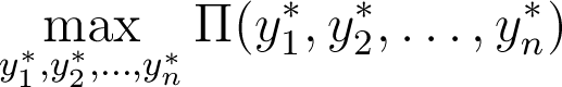
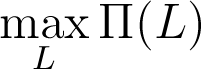
This is a multivariate maximization where each variable is the target of an independent control process. We want to avoid having to explore the whole combination space to find the right target vector, so we are going to condition the targets among themselves to reduce this maximization to a single variable. The main target the firm sets is the number of workers to hire L; this is equivalent to setting the daily production quota f(L). We then set sales targets equal to production (sell everything you make) and buying targets equal to daily inputs (buy everything you need). The maximization problem becomes:

5.17

We use algorithms 1 and 2 to adjust targets after observing profits. Both algorithms are simple hill-climbers to show that no special maximization is required. Both algorithms use little memory, choosing the new workers' target based only the present and the previous one.

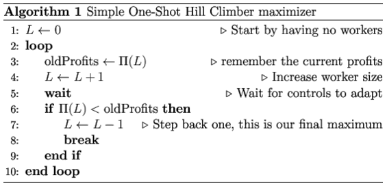
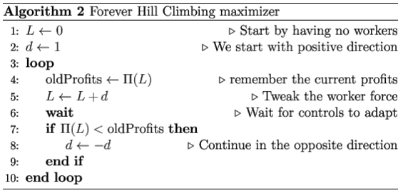
5.18

Line 5 in algorithm 1 and line 6 in algorithm 2 expects the command "wait". This is because controls need time to change policies to achieve the new targets. The wait time can be arbitrary (e.g. one week, one month), but we found it more natural to make it conditional on control achieving targets (e.g. a week after all targets have been achieved). Conditional wait time has the advantage of heterogeneity so that different firms with different controls can use the same maximization algorithm at different frequencies. It is also how we endogenously connects the Hicksian market days to short run.

5.19

Like with control, having zero knowledge has drawbacks. There are two major drawbacks with this maximization procedure: an economic problem and a practical one.

5.20

Trial and error maximization is economically inefficient. Until the profit maximizing targets are found, the firm spends time either under or over-producing. This performance can influence the decision and profitability of suppliers, clients and competitors which are also groping for the right targets. If we allow agents to make mistakes, there will be consequences.

5.21

This maximization is also susceptible to noise due to competition. Both algorithm 1 and 2 are hill-climbers: they compare today target's profits with the previous target's profits. Implicitly we are assuming that if we were to revert back to the old target we would earn the old profit. This stops being true when competitors are concurrently changing their targets. The maximization algorithm thinks it is maximizing ∏(L) but it is actually maximizing ∏(L_i, L_−i) with no control or knowledge of opponents' workforce L_−i. Each agent decision shifts everybody else's profit function. As a setup it is similar to the "Moving Peaks Benchmark" problem (Blackwell & Branke 2006) except that peaks are shifted endogenously by each agent rather than by stochastic shocks.

5.22

In spite of this we show in the competitive example that the resulting noise is manageable. It stops agents from approaching any steady state, but it does not stop them from approaching equilibrium prices.

Zero-Knowledge Firm Examples

Mathematical Example

6.1

In this example we use no software. Prices and quantities are continuous. A zero-knowledge firm hires workers from a market with daily labor supply L = 2w, it has daily production function q = L, and faces the daily demand function q = 100 − 5p. The firm is composed of two departments, a HR department hiring workers and a sales department selling goods. The departments act daily, in parallel and independently. The firm maximizes arbitrarily every 10 days using algorithm 1.

6.2

For the first 10 days, the target number of workers is 1. The next table shows the HR PID process.

Table 3:
Day	HR's et	HR's	Wages (ut)	Workers to Hire (yt*)	Workers Hired' (yt)	Daily Production
1	-	-	0	1	0	0
2	1	1	.250	1	5	.5
3	.5	1.5	.325	1	.650	.650
4	.350	1.850	.388	1	.775	.775
5	.225	2.075	.426	1	.853	.853
6	.148	2.223	.452	1	.904	.904
7	.096	2.319	.469	1	.937	.937
8	.063	2.382	.479	1	.959	.959
9	.041	2.423	.487	1	.973	.973
10	.027	2.450	.491	1	.982	.982

6.3

At the same time the sales department is using its own PID controller to sell products. The target sales is equal to daily production (which is driven by the HR department) plus leftover inventory. For this example we force initial sale price to be 20.

Table 4:
Day	Sales' et	Sales'	Sale Price (ut)	Daily Production	Goods to sell (yt*)	Customers Attracted (yt)
1	-	-	20	0	0	0
2	0	0	20	.5	.5	0
3	-.5	-.5	19.875	.650	1.150	.626
4	-.525	-1.025	19.769	.775	1.3	1.156
5	-.144	-1.169	19.759	.853	.996	1.205
6	.208	-.960	19.818	.904	.904	.908
7	.004	-.956	19.809	.937	.937	.955
8	.018	-.938	19.813	.959	.959	.934
9	-.025	-.963	19.806	.973	.998	.970
10	-.029	-.992	19.800	.982	1.011	.999

6.4

At the end of Day 10 the maximization algorithm is called and compares profits with 0 workers (which is 0) against the profits with 1 worker target. The firm paid .491 in wages to .982 workers, for a total cost of .482; the firm produced .982 goods sold at 19.8 a unit for a total revenue of 19.443. The firm's daily profits then are 18.961. Because increasing workers increased the profits (from 0 to 18.961) the maximization algorithm sets the new worker target to be 2. 2 is set as target to the HR department from Day 11, restarting the loop.

A Monopolist Example

6.5

There is a single firm with two departments: a sales department and an HR department. There is a fixed daily demand for goods as shown in the next figure. The demand is step-wise and discrete. The firm also faces a step-wise discrete supply curve made up of individual workers' reservation wages. The firm must pay a single wage to all employees which explains why the marginal cost curve is steeper than the wage curve (the second worker has reservation wage $16, but hiring him requires raising the first worker wage by $1, hence the marginal cost is $17).

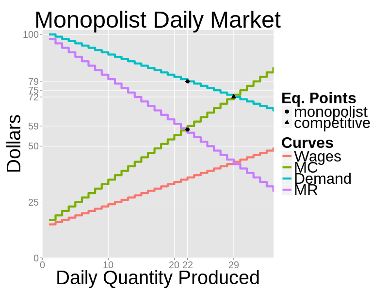
Figure 12. The daily demand faced by the monopolist, the wage curve and the resulting marginal cost curve

6.6

Production is constant returns: each worker produces 1 unit of good every day. There is no capital, no fixed costs and no other inputs. Market is an order book. Everybody places limit orders and crossing order are automatically filled. The trading price is always the price quoted by the seller. Prices and quantities are always natural numbers. A rational monopolist maximizes profits by hiring 22 workers. The rational monopolist price is $79.

6.7

The zero-knowledge firm has none of this information. The firm has no knowledge of being a monopolist either. Initially the wage offered is set to 0, the sale price is set to 100. The maximization used is algorithm 1. The maximization wait time is endogenous: 3 weeks after the labor targets have been filled by the HR department.

6.8

The firm's daily production and sale price in a sample run are shown in the next two figures. The zero-knowledge firm acts rationally in spite of no knowledge, uncoordinated departments and rudimentary maximization.

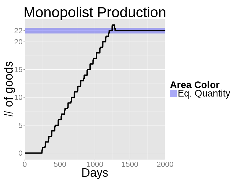
Figure 13. Daily production in a sample run with a single firm

6.9

Notice in price plot the same temporary undershooting as in the zero-knowledge seller example; this undershooting has a different cause: the sales department PID has no foreknowledge of different changes in worker targets. In a way the sales department is continually surprised by changes in production and its PID controller has to catch up. It is the cost of using completely reactive control and total departmental independence.

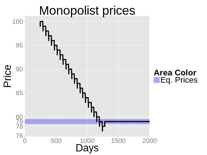
Figure 14. Daily production in a sample run with a single firm

6.10

The results are only slightly different if we use algorithm 2. In this case the firm forever oscillates between hiring 21, 22 and 23 workers ad libitum.

Competitive Market

6.11

We replicate the market of the previous section and add competition. In this example there are 5 firms in the market. Nothing changes in the internal structure of the firm. The firms have no knowledge of having competitors. Each firm follows algorithm 2 to maximize. The competitive equilibrium price would be $72 and the equilibrium daily production would be 29.

6.12

The next two figures show a sample run. Unlike the monopolist case, the results are more noisy and do not stabilize. Both the quantity traded and the prices orbit around the equilibrium values, but they never settle.

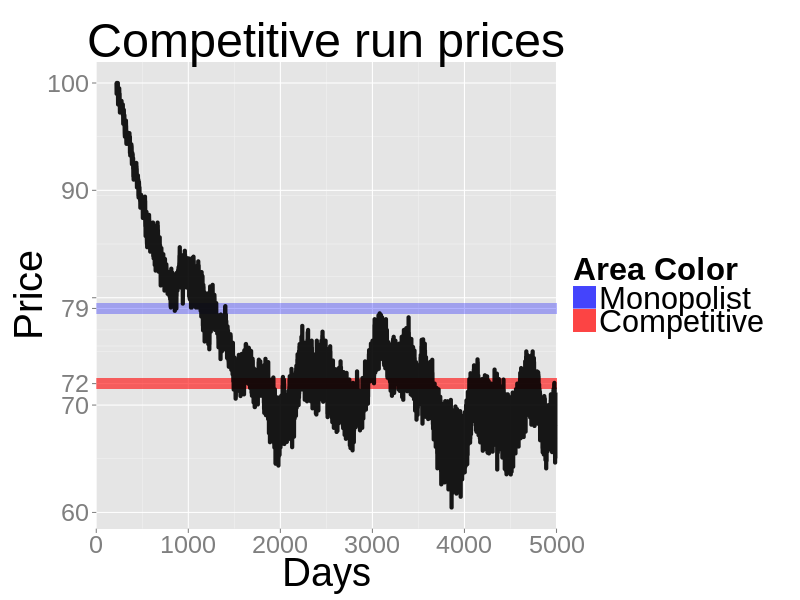
Figure 15. Daily production in a sample run with a single firm

6.13

Compared to the monopolist scenario production is higher and prices are lower, which is what we expect from economic theory.

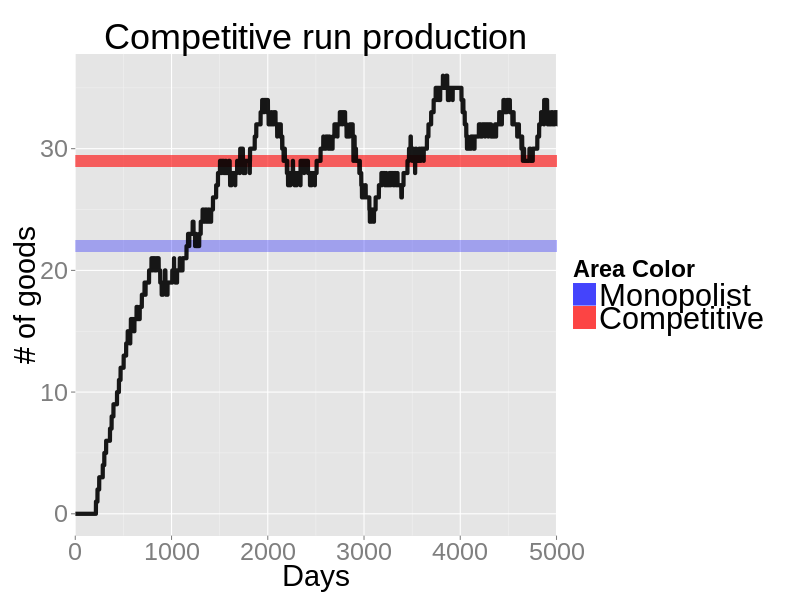
Figure 16. Daily production in a sample run with a single firm

6.14

We run the competitive model 5000 times changing only the random seed. We stop each simulation after 5000 days and record final price and quantity. The next figure shows the distribution of results. While dispersed, all observations cluster around the market demand function. This shows how with competitive noise, control keeps performing well in keeping production and price linked even when the maximization fails to find the profit maximization quantity.

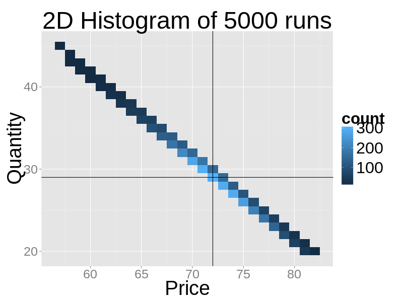
Figure 17. The 2D histogram of price-quantity results of 5000 sample runs of the competitive scenario

6.15

If we focus on prices alone, we can see that almost all the simulations with competition prices are lower with competition than with monopoly.

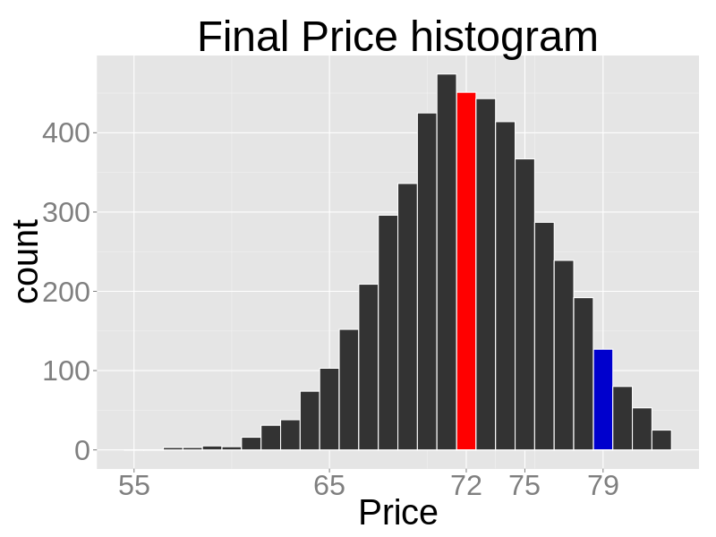
Figure 18. The histogram of prices from 5000 competitive runs. The red bar represents the theoretical competitive prices, the blue bar the theoretical monopoly prices

Conclusion

7.1

We introduced a new way to model decision making that works, is easy to expand and requires no informational assumption. In doing so we have made some assumptions that are questionable and can be improved on.

7.2

First, we have decided that firm's trial and error is done over prices. Thanks to economics surveys by Blinder (1998) and Fabiani et al.(2006) we know that price flexibility is uncommon. Prices are more like targets, changing perhaps three times a year.

7.3

Second, while zero-knowledge firms are created to show how agents can bootstrap correct behavior without looking at prices, there is no reason to assume agents are so autistic. Benchmarking is common-place in any industry. A more realistic model would use more feed-forwarding and, more importantly, more nuanced optimization.

7.4

Third, we assumed that demand reacts immediately to changes in prices. This is in line with usual economic assumptions but it has the additional advantage of avoiding the complicated design of controllers that deal with delays between policy changes and results.

7.5

In spite of its simplicity, agents with this behavior can provide a simple baseline on which to build economic agent based models.

Notes

¹ The source code to run all these examples is available at https://github.com/CarrKnight/MacroIIDiscrete

References

ÅSTRÖM, K. J., & Hägglund, T. (2006). Advanced PID control. ISA-The Instrumentation, Systems, and Automation Society.

AXTELL, R. (2005). The Complexity of Exchange*. The Economic Journal, 115(504), F193– F210. [doi:10.1111/j.1468-0297.2005.01001.x]

BAGNALL, A., & Toft, I. (2006). Autonomous Adaptive Agents for Single Seller Sealed Bid Auctions. Autonomous Agents and Multi-Agent Systems, 12(3), 259–292. [doi:10.1007/s10458-005-4948-2]

BLACKWELL, T., & Branke, J. (2006). Multiswarms, exclusion, and anti-convergence in dynamic environments. IEEE Transactions on Evolutionary Computation, 10(4), 459 –472. [doi:10.1109/TEVC.2005.857074]

BLINDER, A. S. (1998). Asking About Prices: A New Approach to Understanding Price Stickiness. Russell Sage Foundation.

CHEN, X., & Deng, X. (2006). Settling the Complexity of Two-Player Nash Equilibrium. In 47th Annual IEEE Symposium on Foundations of Computer Science, 2006. FOCS '06 (pp. 261–272). [doi:10.1109/FOCS.2006.69]

CLIFF, D., Bruten, J., & Road, F. (1997). Zero is Not Enough: On The Lower Limit of Agent Intelligence for Continuous Double Auction Markets. HP Laboratories Technical Report HPL.

CURRIE, M., & Steedman, I. (1990). Wrestling with Time: Problems in Economic Theory. University of Michigan Press.

DENG, X., Papadimitriou, C., & Safra, S. (2002). On the Complexity of Equilibria. In Proceedings Of The 16Th Annual Symposium On Theoretical Aspects Of Computer Science (pp. 404–413). [doi:10.1145/509907.509920]

DOSI, G., Fagiolo, G., & Roventini, A. (2010). Schumpeter meeting Keynes: A policy-friendly model of endogenous growth and business cycles. Journal of Economic Dynamics and Control, 34(9), 1748–1767. [doi:10.1016/j.jedc.2010.06.018]

FABIANI, S., Druant, M., Hernando, I., Kwapil, C., Landau, B., Loupias, C., … Stokman, A. (2006). What Firms' Surveys Tell Us about Price-Setting Behavior in the Euro Area. International Journal of Central Banking (IJCB). Retrieved from <http://www.ijcb.org/journal/ijcb06q3a1.htm>

FOLEY, D. K. (2010). What's wrong with the fundamental existence and welfare theorems? Journal of Economic Behavior & Organization, 75(2), 115–131. [doi:10.1016/j.jebo.2010.03.023]

GINTIS, H. (2007). The Dynamics of General Equilibrium. The Economic Journal, 117(523), 1280–1309. [doi:10.1111/j.1468-0297.2007.02083.x]

GJERSTAD, S. & Dickhaut, J. (1998). Price formation in double auctions. CiteSeerX. Retrieved from <http://citeseerx.ist.psu.edu/viewdoc/summary?doi=10.1.1.68.6675> [doi:10.1006/game.1997.0576]

GODE, D. K., & Sunder, S. (1993). Allocative Efficiency of Markets with Zero-Intelligence Traders: Market as a Partial Substitute for Individual Rationality. Journal of Political Economy, 101(1), 119–37. [doi:10.1086/261868]

HOWITT, P., & Clower, R. (2000). The emergence of economic organization. Journal of Economic Behavior & Organization, 41(1), 55–84. [doi:10.1016/S0167-2681(99)00087-6]

JAFFE, W. (1967). Walras' Theory of Tatonnement: A Critique of Recent Interpretations. Journal of Political Economy, 75(1), 1–19. [doi:10.1086/259234]

LEIJONHUFVUD, A. (1984). Hicks on Time and Money. Oxford Economic Papers, 36, 26–46.

MÄKI, U. (2008). Economics. In M. Curd & S. Psilos (Eds.), The Routledge Companion to Philosophy of Science (pp. 543–554). London: Routledge.

NOWAK, A., Rychwalska, A., & Borkowski, W. (2011). Why Simulate? To Develop a Mental Model. Journal of Artificial Societies and Social Simulation, 16(3), 12. https://www.jasss.org/16/3/12.html

ORTEGA, M., & Lin, L. (2004). Control theory applications to the production–inventory problem: a review. International Journal of Production Research, 42(11), 2303–2322. [doi:10.1080/00207540410001666260]

PAPADIMITRIOU, C. H. (1994). On the complexity of the parity argument and other inefficient proofs of existence. Journal of Computer and System Sciences, 48(3), 498–532. [doi:10.1016/S0022-0000(05)80063-7]

SCARF, H. (1960). Some Examples of Global Instability of the Competitive Equilibrium. International Economic Review, 1(3), 157–172. [doi:10.2307/2556215]

SMITH, C. A., & Corripio, A. B. (2005). Principles and Practices of Automatic Process Control (3rd ed.). Wiley.