
 Abstract
- Network infrastructures, such as roads, pipelines or the power grid face a multitude of challenges, from organizational and use changes, to climate change and resource scarcity. These challenges require the adaptation of existing infrastructures or their complete new development. Traditionally, infrastructure planning and routing issues are solved through top-down optimization strategies such as mixed integer non linear programming or graph approaches, or through bottom up approaches such as particle swarm optimizations or ant colony optimizations. While some integrated approaches have been proposed int he literature, no direct comparison of the two approaches as applied to the same problem have been reported. Therefore, we implement two routing algorithms to connect a single source node to multiple consuming nodes in a topology with hard boundaries and no-go areas. We compare a geometric graph algorithm finding an (sub)optimum edge-weighted Steiner minimal tree with a Ant Colony Optimization algorithm implemented as an Agent Based Model. Experimenting with 100 randomly generated routing problems, we find that both algorithms perform surprisingly similar in terms of topology, cost and computational performance. We also discovered that by approaching the problem from both top-down and bottom-up perspective, we were able to enrich both algorithms in a co-evolutionary fashion. Our main findings are that the two algorithms, as currently implemented in our test environment hardly differ in the quality of solution and computational performance. There are however significant differences in ease of problem encoding and future extensibility.
- Keywords:
- Ant Colony Optimization, Steiner Minimal Tree, Infrastructure, Routing, Model Comparison
Introduction
- 1.1
- This paper explores the similarities and differences of two
very different algorithms to plan and route infrastructures. On the one
hand we will use a geometric graph algorithm, and on the other
an agent based implementation of an ant colony optimization.
Before diving into algorithm comparisons, we will discuss networked
infrastructures and the challenges that their design and routing
present.
Networked infrastructures
- 1.2
- Networked infrastructures, such as gas pipelines, fresh water pipelines, power grid, glass fiber networks, roads, railroads and waterways form the backbones of our society as they provide essential utilities and services. These infrastructures can be understood as Large Scale Socio-Technical systems (Bijker et al. 1987) that have been evolved over decades and enable suppliers and consumers of goods and services to connect (Chappin 2011). These systems are facing challenges as changes in the social realm, such as liberalization and unbundling affect the way infrastructures are operated, and in the technical domain as quantity and quality of demand change. At the same time these large systems experience the effects of climate change and increasing resource scarcity. Many countries have developed policies to increase the energy efficiency of the infrastructure systems in place and adopt more sustainable technologies (IPCC 2007). Rising to these sustainability challenges requires that existing infrastructures are adapted, for example by modifying the topology of the power grid to accommodate distributed generation, or that entirely novel infrastructures must be created. Examples of such new infrastructures are a CO2 infrastructure for carbon capture and storage (CCS) of large CO2 sources in an industrial area (Viebahn et al. 2009), a heat infrastructure that connects excess supply of industrial heat to nearby heat consumers and an infrastructure of biogas pipelines that pool the output of individual farmers (Heijnen et al. 2013).
- 1.3
- The planning and roll-out of these new networked
infrastructures is challenging for a number of reasons. Firstly,
they are, more often than not, placed in densely built and highly
urbanized environments near infrastructure users. Because of this,
they exist in a multi-actor context, with various social actors
involved in planning, development, maintenance and the direct
effects and benefits of such infra. Secondly, they are very capital
intensive and long-lived, meaning that the return on investment
comes long after the up-front cost are made. Finally, their
perceived costs and benefits are strongly observer-dependent. How
"good" an infrastructure is depends on who pays the costs, who
receives the revenues and how the risks are distributed (Dixit & Pindyck 1994). At the end of the day all these issues present challenges
for planning infrastructures, which may well lead to inferior
infrastructure layouts or even valuable infrastructures not being
built at all.
Routing challenge
- 1.4
- The issues presented above exist in all stages of the
infrastructure development process, but are nowhere more visible
than in the routing stage. The exact choice of the route will
greatly affect the property prices near and at the route,
potentially leading to land price speculation further affecting the
local inhabitants. An of course, exact routing choices directly
affect the technical difficulty and cost of the project. It makes a
big difference whether a pipeline passes a short distance through a
flat grassland or if it meanders through rivers, tunnels and
through cities for many kilometers. Infrastructure routing is
therefore an important and challenging aspect that warrants further
exploration. In this paper we will focus on obstacle avoiding and
cost minimization aspects of the routing problem.
Top-Down versus Bottom-Up approaches
- 1.5
- In the literature one can discern two main approaches to the infrastructure routing problem, namely Top-Down and Bottom-Up. By Top-Down we understand approaches that rely on a global optimization algorithm of some type, which uses complete information about the system to find a global optimum. There are several excellent examples of Top-Down approach. Middleton & Bielicki (2009) offer a comprehensive routing approach for CO2 capture and storage, based on an mixed integer linear programming algorithm, taking many technical and social criteria into consideration. Kabirian & Hemmati (2007) offer a nonlinear optimization approach over a long time horizon for planning gas pipelines, optimizing over many technical and economic factors. Marcoulaki et al. (2012) provide a stochastic optimization integrated with GIS to obtain an optimum routing for oil and gas pipeline infrastructure. Park & Storch (2002) describe a very detailed CAD based pipeline routing optimization algorithm for ship engine room pipeline routing, based on material properties, spatial constraints and human accessibility limits. When dealing with routing around obstacles, graph approaches are common and useful (Gastner & Newman 2006). For example, Hwang & Richards (1992) give a overview of graph approaches to routing. Wu et al. (2007) present an rectilinear Steiner minimal tree algorithm for obstacle avoiding, applied to telecommunication network routing. While these examples differ in their scope and design target, they all have the Top-Down perspective in common. Given a set of multidimensional constraints, they attempt to locate a single point optimal solution.
- 1.6
- On the other side of the conceptual spectrum, we find the Bottom-Up approaches, which use distributed entities, using local information to achieve a "good enough" solution in a multidimensional design space. Ant colony optimizations (ACO) are commonly used for various routing and scheduling problems in engineering domains and in electronics and computers (Chandra Mohan & Baskaran 2012), and therefore they are applicable for finding the optimal network layout. For example, Maier et al. (2003) present an ACO algorithm for the design of water distribution systems. Qin et al. (2012) present a ACO variant for optimizing logistics routing. Geem (2009) uses a particle swarm optimization algorithm to explore the design space of water distribution systems. Arnaout (2013) further generalizes the ACO algorithm to deal with network infrastructures with an unknown number of elements. What these examples have in common is that they use a distributed approach based on ACO or similar algorithms to explore the design space of infrastructures.
- 1.7
- While both approaches are useful in their own right, they
generally have different advantages and disadvantages. The main
advantage of the Top-Down approach is that it guarantees a
solution, usually computed quickly, whereas the Bottom-Up approach
can work with incomplete information and are often very intuitive
when describing the problem. The main disadvantage of the Top-Down
paradigm is the requirement for complete information about the
system in order to perform the optimization and the difficulty in
encoding the problem. The main disadvantage of the Bottom-Up
paradigm is that such algorithms do not guarantee an optimal
solution and tend to be very computationally inefficient. While
these advantages and disadvantages are understood in general, there
is a lack of literature directly comparing the two approaches when
applied to the same problem. There are however several examples in
literature attempting to combine these two paradigms. A combination
of the graph theoretical and ACO approach has been explored by
Hu et al.
(2006). Their approaches focuses on routing in rectilinear
graphs, as present in integrated circuit design. Liu & Wang (2012) explore multi-terminal
pipe routing by Steiner minimal tree and particle swarm
optimization. These examples present an integrated approach, but do
not explore the similarities and differences of the two approaches
explicitly. We aim to compare these two approaches and to explore
their advantages and disadvantages when applied to a single
problem.
Problem delineation
- 1.8
-
In this paper we will apply the two approaches to the same problem
- routing of infrastructures, compare the algorithms, analyze their
respective merits and explore the lessons learned across the two
approaches. We will apply both algorithms to a class of
infrastructure planning problems in which one source needs to be
connected to various sinks in a two-dimensional area in which only
a part of the area may be used for the infrastructure network. In
order to make a feasible comparison, we simplify the problem of
infrastructure network planning to show only the following
aspects:
- Networks transport a commodity from one source to several sinks.
- The building costs depend to a large extent on the pipeline length (e.g. due to digging costs), but also on the pipeline capacity (e.g. due to materials costs).
- The networks need to be built in areas that pose limitations on the possible routing of pipelines due to existing buildings, obstacles like rivers or mountains, or zoning rules (e.g. protected natural areas).
- 1.9
- We formulate the simplified planning problem as an optimization
problem with the objective to minimize the expected building cost,
taking into account the various aspects and constraints of the
system. We will argue that the other uncertainties mentioned, such
as uncertainties in the participating actors in the network,
uncertainties on potential future expansion with the possible
extensions to the models presented, can be included in one or both
of the approaches, see for instance (Heijnen
et al. 2013). Having identified the problem, we will explore the two used
algorithms in more detail.
Tale of two algorithms
- 1.10
- Geometric graph theory (GGT) is a specialization of graph theory and studies geometric graphs. A geometric graph is a graph structure consisting of nodes and edges, where the nodes are points in space and the edges are straight lines between these points (Pisanski 2000). Geometric graph theory combines geometric and topological methods to solve various problems on these geometric graphs. While graph theoretical approaches are not usually considered to be Top-Down, in this case the method considers the system in its totality, and has perfect information on all elements. Therefore, we will consider it as a Top-Down method in this work. The specific lay-out of a network as described above can be seen as a geometric graph. Heijnen et al. (2013) developed a practical method to find a minimum cost network lay-out for a given set of nodes within a bounded region. The method combines various heuristics from geometric graph theory. In general when the physical coordinates of the nodes to be connected are known, the Euclidean minimal spanning tree or Steiner minimal tree are trees in the Euclidean space that connect all nodes and minimize the total length of all connections. Because our network costs depend not only on the connections lengths but also on their capacities, we need to find an edge-weighted Steiner minimal tree (EWSMT). Thomas & Weng (2006) propose a heuristic to determine that tree for unbounded regions, which Heijnen et al. (2013) combined with the approach in (Lee & Preparata 1984) for closed regions. This approach can therefore be used to find the optimal network layout in the problem setting defined above.
- 1.11
- Agent-Based Modeling (ABM), is a Bottom-Up method in which a collection of heterogeneous, intelligent, and interacting agents [...] operate and exist in an environment, which for its part is made up of agents (Epstein & Axtell 1996). The interacting agents generate emergent patterns of complex dynamic behavior (Borshchev & Filippov 2004). One specific way to use an ABM is to implement an ant colony optimization (ACO) algorithm, which approaches optimization problems through digital "ants", moving across a graph, laying pheromones and search for food (Sammut & Webb 2011). Ant agents only have access to local information from their immediate surroundings, and have no notion of best or worst paths. Paths are an emergent property, arising from ant interactions.
- 1.12
- Ant colony optimizations conceptualize the problem as a graph
and the overall objective is to find the optimal solution from the
set of candidate solutions (Dorigo &
Di Caro 1999). A candidate solution is a selection of the
edges from the graph that meets all constraints. The procedure of
an ant colony optimization in general has three parts, one in which
ants execute their behavior, e.g. they decide to move ahead, one
which the ant's environment responds to changes, e.g. where
pheromones are evaporated, and the so-called deamon actions, in
which centralized decisions are made, e.g. where partial solutions
are frozen. The latter is optional. The agents - or ants - build
solutions by moving on the graph. Agents have a memory of their
movements and their moving behavior can be guided by the
constraints. The agents may interact indirectly by dropping
pheromones. Good quality solutions emerge as the result of a vast
number of ants and their indirect interaction.
Approach and paper structure
- 1.13
- As already mentioned, we aim to compare the two approaches in order to explore their strengths and weaknesses. We do that by using the geometric graph method from (Heijnen et al. 2013) and by developing an ABM ant colony optimization, using the same inputs. We develop a general comparison structure, by generating 100 random regions with one source and several sinks that vary in capacity and location. The algorithms will be compared on the ability to converge to a feasible solution, the network layout and cost and the computational performance. Furthermore, the approaches are compared on ease of implementation and expansion. The paper is structured as follows. In section two we formally define the problem and describe the implemented algorithms. In section three we describe the experimental setup for comparing the algorithms. In the fourth section we compare the simulation outcomes and discuss the two approaches. We end the paper with conclusions and an outlook in section 5.
Problem and algorithm
specification
- 2.1
- In this section we formally describe the problem and both
algorithms. We start with a formalization of the problem and the
translation of the problem to a form that the algorithms can cope
with it.
Problem formalization
- 2.2
- The following optimization problem needs to be solved:
Find a network that minimizes the total building cost,
satisfying the following three constraints:
- The network connects all consuming nodes to the source
- All connections must go through the allowed region
- The pipeline capacities satisfy the demands of the consuming nodes
- 2.3
- In order to compare the approaches, they share the following
inputs:
- The location of the participants in the network, given by their coordinates in the two dimensional plane. The nodes are ordered from 1 to N, where node 1 in all cases represents the source.
- The demand qi, given for each consumer node, 2≤i≤N. We assume that the source can always satisfy the total demand of all consumer nodes.
- The boundaries of the allowed region and the possible obstacles, given as ordered lists of the corners' coordinates.
- The cost function f (q) = qβ, which is the cost per length unit of a connection in the network with capacity q. The cost function is chosen as in (Thomas & Weng 2006), defining the cost of building a pipeline e as Ce = leqeβ. Here le is the length of e and qe is the total capacity of pipeline e. The exponent β is the cost exponent for the capacity with 0≤β≤1. If β = 0, the capacity of the pipelines has no influence on the costs. If β = 1, building two pipelines of capacity 1 is just as expensive as building one pipeline of capacity 2. The total investment costs Ctotal(T) of a network T is the sum of all edge costs. where E(T) is the set of all edges in the network T.
Geometric graph method
- 2.4
- From a geometric graph perspective, this problem translates to
finding an edge-weighted Steiner minimal tree that connects all
consumer nodes to one source within a bounded region, avoiding
possible obstacles. A geometric continuous 2D-plane represents the area and a
weighted graph with N nodes
represents the network. The first node is the source. The other
N - 1 nodes are the consuming
nodes that need to be connected to this source node. The given list
of coordinates in the 2D-plane sets the position of the nodes in
the graph. The edges in the graph represent the pipeline
connections between the nodes. The length le of each edge e is the Euclidean distance between its two
end nodes. The weight of the edge e in the graph represents the capacity
qe of the connection.
The building cost of a connection e equals
Ce =
leqeβ
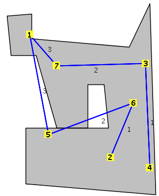
as defined before. A simple polygon with the given corner points
defines the allowed region. Also, the obstacles are represented by
simple polygons. To include these obstacles in the allowed region,
a new extended simple polygon is defined by introducing new edges
that 'cut' open the polygon, see figure 2.1.
Agent-based modeling
- 2.5
- The agent-based ACO approach translates the problem to finding a connected set of discretized patches that link all consumer nodes with the source at the lowest network cost. The area represents the region using patches of 1 by 1 unit of length. The source is represented by an ant nest on the patch with the given coordinates. Food sources represent the consumer nodes on the corresponding patches. Using patches is superficially different from a standard ACO representation, which considers the system as a graph (Dorigo et al. 1996). Fundamentally, however, there is no difference, because a two-dimensional space consisting of patches is equivalent to a graph, where the patch is a graph node that has 8 links to all neighbors.
- 2.6
- A network connection between two nodes is defined as a list of
connected patches. The observer calculates the additional network
costs of building a new network connection. The length of the
connection equals the sum of the distance between all neighboring
patches in this list. Patches can be side neighbors when they
share one side or corner neighbors when they share one corner. The
distance between two neighboring patches equals 1 or
 ,
respectively.
,
respectively. - 2.7
- The building cost Cp of adding patch p to the network equals then
- in which SNp and CNp are the sets of side neighbor and corner neighbor network patches of patch p, respectively. The total cost Cpatch(P) of building a network P is now the sum of the building costs Cp of all patches p in the patch network P.
- in which SNp and CNp are the sets of side neighbor and corner neighbor network patches of patch p, respectively. The total cost Cpatch(P) of building a network P is now the sum of the building costs Cp of all patches p in the patch network P.
- 2.8
- Patches located outside the allowed region bring extremely high
building cost to avoid that they become part of the network.
Rp denotes the regional
building cost for a patch p. Ants
record the capacity required by the consumer node found and the set
of patches on their return path to the source, attracted by the
scent of the nest/source node. The network is built in steps. Each
patch p records the existing
network capacity, given by qp.
Algorithm description
- 2.9
- The details of the GGM algorithm are available in Heijnen et al. 2013, and
the ABM code can be downloaded from
http://www.openabm.org/model/4134.
Geometric graph method
- 2.10
- The geometric graph method defines an initial network using a non-crossing spanning tree that connects all nodes and has the required capacities as weights on the edges. This initial tree is used to search for improvements. This tree network satisfies both the first (all consuming nodes connected to the source) and third constraint (sufficient capacity). Each change of the network will preserve these properties. To satisfy the second constraint (remaining within the allowed region), all edges in the network that lie partly outside the allowed region, represented by the simple polygon defined before, are redirected to their shortest path within the simple polygon using the method from (Lee & Preparata 1984). This replacement is repeated after every change of the network. If connections partly join, the capacity of the joined part is the sum of the original two capacities.
- 2.11
- In each step, the existing network is locally changed as long
as a network with lower total building cost is found. The
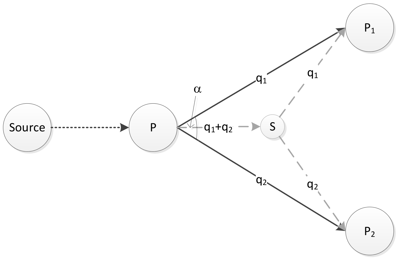
improvements are based on the observation that it is profitable to
partly join two adjacent connections if their interior angle is
small, i.e. smaller than the angle constraint given in (Thomas & Weng 2006) and illustrated by figure
2.2. There the angle constraint reads
cos(α)≤ 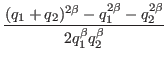 .
.(3) - 2.12
- If the angle α in figure 2.2 satisfies this constraint, adding the splitting point S will be profitable. Using a geometric approach, the optimal location of this so-called Steiner point can exactly be determined (see (Heijnen et al. 2013) for more details). The procedure guarantees that a local minimum is found, since the total building costs decrease after each change of the network.
- 2.13
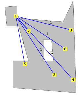
- Figure 2.3 shows an
example of an initial network, in this case the star network,
with the source node 1 as the center, an intermediate network after a few local
improvements and the final result. The initial tree and the order
in which the local improvements take place determine the final
result and it is not guaranteed that the global minimum cost
network will be found. However, within the given topological
structure of the network, the method guarantees that splitting
point locations are optimal with respect to minimizing the cost.
Figure 2.3: Transition from initial to minimal cost network using the geometric graph algorithm Intermediate network
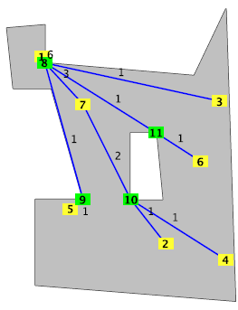
(Sub)minimal cost network
Agent-based modeling
- 2.14
- As is usual in an ACO, the agents are the ants looking for food
sources (the consumer nodes) by a semi-random walk. If they have
reached a food source, they are allowed to return to the nest (the
source node) immediately. On their return they are attracted by the
scent spread by the nest, and the pheromone that fixed network
paths emit. When ants reach the existing network, they will only
follow existing network patches until they reach the nest. The ant
keeps track of the patches it follows back to the nest. When an ant returns to the nest, the observer calculates the
additional costs of adding this path to the existing network using
equation (2) and the observer stores
the path if it is the cheapest so far. The network connection
between the nest and this food source is built when a specified
number of ants have returned from the same food source without
finding a cheaper alternative. When a network connection is built,
the patches that are part of the new connection store the network
capacity for this food source. If the patch was already part of the
network, the capacity is increased accordingly. After this, the ant
will look for food again. The pheromones that the network emits
evaporates and diffuses according to the respective parameter
settings. Even though the ants are allowed to walk through the
no-go area, the no-go area is not attractive for various reasons.
There the evaporation rate of pheromones is immediate and the
building cost for a no-go patch is one thousand times higher than
on an allowed patch. Therefore, when the ant returns to the nest it
is unlikely to follow a pheromone scent across a no-go area and any
path containing a no-go patch is very unlikely to be the cheapest.
The run stops when all consuming nodes, i.e. the food sources, are
connected to the source (the ant nest).
Startup phase
- 2.15
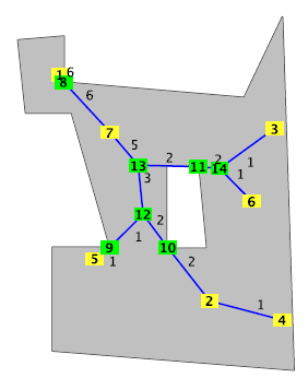
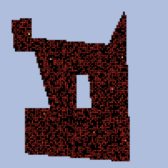
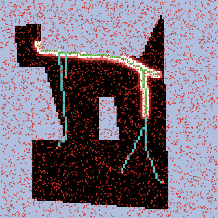
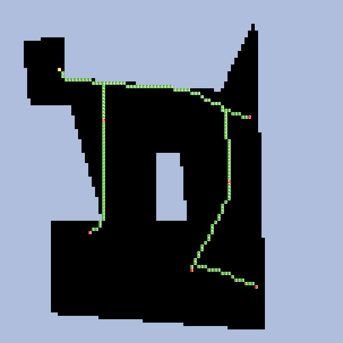
- The first panel of figure 2.4 shows the
algorithm in progress, starting with no network and ants randomly
distributed over the entire area. In the second some of the connections are already established and ants, returning
from other food sources, are attracted to the paths, reusing these
connections. The third panel shows an example of the final network.
Parameterizing the ACO/ABM
- 2.16
- The agent-based implementation of the ACO uses 15 different
parameters that influence the behavior of the ants directly or
indirectly. Finding an optimum setting in this parameter space is
non-trivial. Previously, ACO parameters have been estimated by
genetic algorithms (Altiparmak
& Karaoglan 2007) or they have been estimated by hand. In
table 2.1 we present the
explored parameter ranges. Parameter settings are varied for each
parameter individually and the experiment was repeated N times. The
other parameter values are fixed, see table 2.2. The overview of all
ACO ABM parameters used is presented in table 2.3 for the boolean parameters and
in table 2.4 for continuous
ones.
Table 2.1: Explored parameter ranges Parameter Min Step Max Fixed value N patience 0 10 240 50 121 population 1000 100 10000 4000 455 diffusion_rate 0 2.5 100 25 205 evaporation_rate 0 2.5 100 15 205 wiggle_angle 1 5 176 45 180 wiggle_probability 0.1 0.01 0.99 0.1 450 nest_scent_power - - - - - pheromone_network_multiplier 0 1 100 1 505 pheromone_network_power pheromone_walking_power 0 10 1000 303 pheromone_carrying_power 0 10 1000 303
Table 2.2: Correlation results Parameter Min Max Corr. Costs p Corr. Time p patience 0 240 -0.28 0.00 0.98 0.00 population 1000 10000 0.48 0.00 -0.80 0.00 diffusion_rate 0 100 0.02 0.38 0.08 0.22 evaporation_rate 0 100 -0.26 0.00 -0.14 0.05 wiggle_angle 1 176 -0.11 0.14 0.68 0.00 wiggle_probability 0.1 0.99 -0.18 0.00 0.19 0.00 pheromone network multiplier 0 100 0.02 0.35 -0.19 0.00 pheromone walking power 0 1000 0.05 0.26 -0.13 0.03 pheromone carrying power 0 1000 -0.21 0.00 -0.50 0.00 - 2.17
- Based on the explored parameters and their correlations, we
have used the following reasoning to determine individual parameter
values.
- When the patience value is low, (up to approx. 50), the costs are sometimes very high, and are reduced as the patience further increases. Above 25 there does not seem to be much effect on cost, but the computational time rises linearly with it. Therefore patience = 50.
- Higher population leads to higher costs and lower time. Relation is not linear and has an inflexion point between 4000-5000 Thus, population = 4000.
- Diffusion rate seems to have no effect on the costs or time, which is surprising. Average setting diffusion-rate = 25
- Evaporation rate should not be 0, but it seems to have little effect on the costs. It has a minimum time around 15. Thus evaporation-rate = 15
- The wiggle angle does not affect the costs, but with high angles the time increases significantly. We choose it not too high, thus wiggle-angle = 45
- The wiggle probability hardly has an influence on the costs or the time, possibly due to chosen low wiggle-angle. At high wiggle-angle the wiggle-probability has an influence on time, but not the costs. An experiment where we varied both clearly shows that the time is lowest at low angle and low probability. Other combinations still hardly affect the costs. Thus wiggle-probability = 0.1
- Pheromone-network-multiplier gives a good balance between two topologies, star network and minimal spanning tree. Pheromone network power is derived from this parameter. Pheromone-network-multiplier = 5.
- Pheromone walking power and pheromone carrying power are only used in an ACO configuration that is not applicable to our case, and are thus not set.
Table 2.3: Boolean parameters specific to the agent-based method. Parameter Description Values Influence Move-to-center Despite the fact that the system is represented as patches, the ants move continuously over the 2D plane. When this setting is enabled, the space is also discretized in the behavior of the ants. False When enabled, the paths of the ants are straighter, but the variability is too low, making the location of network joints worse. Jump-to-nest Normally, ants move one step per time tick. When enabled, the ants walk back to the nest immediately after a food source is found. True Disabling this setting gives an advantage to food sources close to the nest. Enabling leads in general to better results. Relocate-at-reset Ants start each search from the nest (except for the start of the simulation). When enabled, ants are given a random location after they have returned to the nest. False Enabling has no influence on the end results. Pheromone-network When enabled, the network emits a fixed amount of pheromone to attract the ants on their return. True Enabled, the ants will more easily connect to existing network parts and parallel paths are avoided. Pheromone-carrying When enabled, ants emit pheromones when they carry food, which attract other ants to follow their paths. False Despite the fact that this is very common in ant colony optimizations, its function is replaced by the pheromone emitted by the network. When enabled, the strength of the pheromone needs to be set as well. Pheromone-walking When enabled, ants emit pheromones when they are looking for food, which attract other ants to follow their paths. False Despite the fact that this is very common in ant colony optimizations, its function is replaced by the pheromone emitted by the network. When enabled, the strength of the pheromone needs to be set as well.
Table 2.4: Input parameters specific to the agent-based method. Parameter Description Values Influence Population The total number of ants in the simulation. 4000 A rather high number of ants is used to balance the computational time of the ants, the patches, and the observer. Patience The number of ants that need to return from a food source without improvement to the network before the cheapest connection is fixed. 50 Increasing the patience would generally improve the result, but also slows the simulation down. Wiggle-probability The probability that ants will wiggle when searching for food. 0.1 A high wiggle probability negatively influences the time, but has hardly any advantage on the cost. Wiggle-angle The maximum angle that ants wiggle will be normally distributed with average 0 and standard deviation the value of the parameter wiggle angle. Ants change their direction according to that angle. 45 A too small wiggle angle reduces the variability of the ant's paths and therefore the likelihood of finding a good path. Nest-scent-power The strength of the scent emitted from the nest. The nest scent drops down with distance and is 0 on patches which are excluded from the allowed area. 200 This is chosen to be the basis parameter to which the other pheromone values will be related Pheromone-network-multiplier The relative strength of the pheromone emitted by the network. The pheromone level on a network patch is defined as pheromone-network-multiplier ×(nest-scent-power ×(1 - β)). 5 This value gives a good balance between the extreme topologies of a star network, advantageous when β = 1, and the minimal spanning tree, advantageous when β = 0. Pheromone-carrying-strength The strength of the pheromone emitted by ants crying food Not set, since pheromone-carrying is disabled Pheromone-walking-strength The strength of the pheromone emitted by ants looking for food Not set, since pheromone-walking is disabled Diffusion-rate The percentage of pheromones that are diffused each time tick. Not set, since pheromone-walking and pheromone-carrying are disabled Evaporation-rate The percentage of pheromones that evaporate each time tick. Not set, since pheromone-walking and pheromone-carrying are disabled
 leqeβ
leqeβ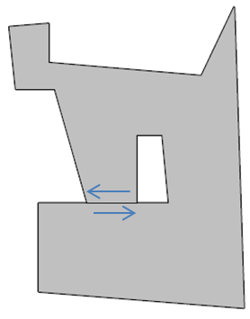
Experiments
-
Experimental strategy
- 3.1
- The Top-Down and Bottom-Up approaches will be compared by
performing algorithm runs on a large number of randomly generated
routing problems, consisting of a random surface area and
source/consumer locations. Each run on the random region will be
repeated a number of times to increase the probability of finding a
good enough solution. The solutions achieved by both algorithms
will be compared on a number of metrics, which will be presented in
§3.2.
Generated set of examples
- 3.2
- In order to compare both methods, we generated 100 random examples
in a 2D-plane of size
100×100 units of length. For each
example, the parameters as listed in table 3.1 are randomly chosen from a
uniform distribution within the given range. A polygon is
generated, which delimits the allowed area. The polygon corners are
randomly put at a location within the total area. One obstacle is
generated with randomly located corners and entirely located within
the polygon. The source and consumer nodes will be located within
the allowed area.
Table 3.1: Input parameters for the 100 generated examples are chosen from an uniform distribution between the ranges displayed. Parameter Range Horizontal axis total area [0, 100] Vertical axis total area [0, 100] Number of polygon corners [10, 30] Number of obstacle corners [4, 6] Number of consumer nodes N [5, 19] Cost exponent β [0, 0.9] Maximum capacity demand D [1, 10] Capacity demand of consumer nodes [1, D]
Repetition
- 3.3
- Both the geometric graph method and the agent-based model run 10
repetitions for each example.
Geometric graph method
- 3.4
-
The geometric graph method can start from any non-crossing spanning
tree ' a network in which all nodes are connected. Out of the ten,
2 are the minimal length spanning tree and the star network with
the source node as the hub (as suggested by (Heijnen et al.
2013), see figure 3.1). Interestingly,
the agent-based model was the inspiration to also include 8
randomly generated non-crossing spanning trees as a starting point
to search the solution space more thoroughly. Outside this random
starting point, there is no stochasticity in the algorithm. A
specific initial tree will always lead to the same solution.
Although the minimal length spanning tree and the star network do
often lead to good networks, sometimes random runs lead to
solutions with network topologies that are overlooked otherwise.
Agent-based modeling
- 3.5
-
The agent-based model builds the network up step by step. Because
the initial locations of the ants and the order in which the ants
act differ between runs, each run leads to different outcomes. The
repetitions increase the chance of a good enough outcome for a
specific geometry.
Comparison metrics
- 3.6
-
The algorithms will be compared on three main areas: availability
of a feasible solution, topology and cost of the resulting network
and computational performance.
Availability of a feasible solution
Geometric graph method
- 3.7
-
Since each intermediate tree in the geometric graph method is a
feasible solution itself, the geometric graph method finds a
feasible solution in all runs, see also figure 2.3.
Agent-based modeling
- 3.8
- Because of stochasticity in the behavioral algorithm of the
ants, each simulation ends with a different network. The simulation
does not guarantee that a feasible network will be
found. The reason for this is that the network path is only fixed
after the patience threshold has been reached. In some extreme
cases is may happen that this path goes through a no-go area. This
may lead to infeasible network routes, even through the chance of
this happening is minimal. See figure 2.4. This means that, overall, the ABM
may find a solution satisfying constraint 1 (see section 2.2) , it may find an expensive
solution that does not meet constraint 2, or it may not find a
feasible solution at all. In order to prevent simulation runs that
spend inordinate amount of time waiting for a minimization of
costs, hard computational limits will be imposed.
Building network cost and topology
- 3.9
-
If a solution is found, it will always be a network with a tree
topology, given the fact that there is only one source connecting
several consumer nodes. However, the resulting topology might show
large variations. The network's topology, the length of its
connections and the exact location of possible Steiner points will
finally determine the network's building cost, which is the main
characteristic to judge the quality of the outcome. Comparison of
the outcome however, is not trivial, since both methods use a
different representation of the resulting tree and also the
building cost are calculated in a different way.
Geometric graph method
- 3.10
-
The output of the geometric graph method represents the network as
a weighted graph in which the nodes are the source, the consumer
nodes, the determined splitting nodes (Steiner nodes) and, if
necessary, some corners of the allowed region. The edges of the
graph represent the pipelines between these nodes. The edges have a
weight equal to the required capacity of the corresponding pipeline
satisfying the demand of the connected consumer nodes. The network
cost is calculated from this graph using equation (1), summing the cost per edge, taking into account
those weights.
Agent-based modeling
- 3.11
- The output of the agent-based method consists of a list of patches
belonging to the network. For each patch, both its location and its
capacity is known. Some patches have more than 2 neighbors that are
also part of the network. These patches are considered as splitting
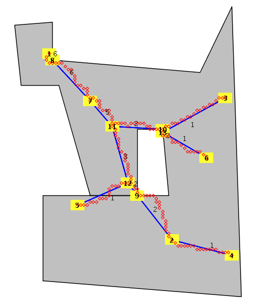
points, or Steiner nodes (see figure 3.2). For the cost calculations,
please refer to section 2.7.
Figure 3.2: Location of a Steiner point and the translation from a patch network to a graph in order to compare the results between the methods. 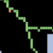
Comparing a graph with a set of patches
- 3.12
- Since both methods represent the solutions differently, some extra steps are needed for a fair comparison between the results. Building cost calculated from a patch list are, for a given topology, always higher than building costs calculated from a graph representation, since in a graph connections are straight and their lengths can unambiguously be calculated. The patch network of the agent-based method can, however, be defined as a graph by adding extra nodes for the identified splitting points and for the possible corners of the allowed region that are part of the network. Following the shortest path through the patches from source to consumer nodes, the edges and their capacity are determined. Figure 3.2 shows an example of the translation result.
- 3.13
- When the location of all nodes and the connections between them
are known, the absolute length le of each connection e can easily be calculated. With these lengths
le,∀e, and with
the capacities of the edges
qe,∀e, the total
building cost is calculated using equation (1). The derived graph and its building cost enable a
fair comparison to the output of the geometric graph method.
Computational performance
- 3.14
- Next to comparing the quality of the generated topologies and their cost, it is important to compare the computational performance of the two approaches. Comparing computational performance across different types of algorithms and across different software environments is a very challenging task. Multiple factors will affect the performance of algorithms, even on identical hardware. The geometric graph method is implemented in Maple 17, while the ABM is implemented in NetLogo 5.0.4. These environments have different general purposes, and thus differences in level of code optimization. While Maple is developed as a computational engine, NetLogo is mainly developed as an educational tool. Furthermore, both packages may well have different levels of optimization of internal libraries making this comparison only valid for the particular implementation in this particular environment. However, in order to get a pragmatic comparison, we will time 1000 simulations runs. Maple is optimized for multicore processing and is able to use 4 out of 8 available compute cores when doing a single run. NetLogo performs an entire run within a single thread, and thus only utilizes a single core. In order to compensate, we will use 4 simultaneous runs of the NetLogo model for the speed comparison.
Results and Discussion
- 4.1
- In this section we will present and discuss the outcomes of the
comparison, based on the presented metrics.
Availability of a feasible solution
- 4.2
- As already discussed, the geometric graph method guarantees a
feasible solution. The ABM ACO algorithm is a search algorithm that
needs to be constrained, since in some cases it will be unable to
find a feasible solution, or take exceptionally long time. In the
ABM algorithm nest observes returning ants, which carry a record
of the route they took. Based on its patience level, it requires a
certain number of ants to return to the nest without lowering the
route cost further. When that patience threshold is reached, the
nest fixes the route and considers it the lowest cost solution. It
can therefore happen that the algorithm either has no route
available at any cost, has a very expensive cost route because it
is going through a no-go area, or has not reached the required
number of ants without finding a lower cost route. We implemented a
computational limitation, forcing the simulation to stop after
100,000 ticks or when the simulation slows down to an average of 20
ticks per second. With these limitations the agent-based method
finds a feasible solution in 99.8% of all runs. The majority of
runs complete much earlier and faster.
Building cost
Geometric graph method
- 4.3
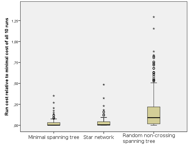
- The geometric graph method was initialized with a minimal
spanning tree, a star network and with 8 randomly generated
non-crossing spanning trees.
Table 4.1: Minimum costs likelihood Likelihood to find the best network starting from GGM Star network 42% Minimal spanning tree 51% Random non-crossing spanning tree 11%
Table 4.2: Cost results of the experiments Correlation coefficient between the network cost and ... Parameter GGM ABM Total number of nodes N 0.33 0.32 Cost exponent β 0.694 0.696 Maximum capacity demand of consumer nodes qmax 0.253 0.258 Mean capacity demand of consumer nodes 
0.262 0.271 Length of minimal spanning tree connecting all nodes 
0.318 0.308 Total variance of cost explained adj. R2 67.5% 67.4% - 4.4
- The results in table 4.1 show that it is useful to include both the runs from these two deterministic trees, but also to add runs starting from several, randomly generated, non-crossing spanning trees. Figure 4.1 shows that the random runs lead to a significantly higher variability in the results.
- 4.5
- Moreover, table 4.2 indicates
that the building cost of the resulting network from one run are
mainly determined by the characteristics of the specific network
problem and are only for one-third influenced by the variability in
the starting tree. All correlation coefficients in table 4.2 are found to be significant at the 0.05
level. This result is not surprising, since the cost of building a
specific network depends to a high extent on the mutual distance
between the nodes (summarized in the total length of the minimal
spanning tree
), the capacity demand of the
consumer nodes (summarized in qmax and
) and the cost of building a
larger capacity connection (given by the cost exponent β). Two good networks connecting the same
nodes using a different topology and different locations for the
Steiner points will therefore only show small differences in
building cost.
Agent-based modeling
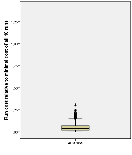
- 4.6
-
The agent-based model used 10 random runs per example to determine
the best networks using the parameter settings from tables 2.3 and 2.4. Figure 4.2 presents the variability in the costs per
example for the ABM runs. Based on the same observation as above,
the final result from one specific run is mainly determined by the
characteristics of the problem and only for one-third influenced by
the stochastic nature of algorithm. Again all coefficients in Table
4.2 are significant at the 0.05
level.
Performance
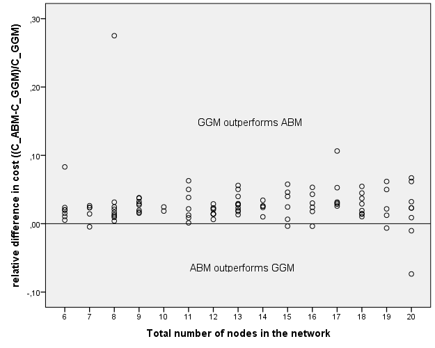
- 4.7
-
We selected the best performing run from 10 runs of the ABM and
compared it with the best GGM out of 10 different initial trees.
The geometric graph method finds in 94% of the 100 examples a
network with building cost equal to or lower than the agent-based
method. However, the differences were mostly small, 3% on average
(with a standard deviation of 3%) of the minimal building cost
resulting from the best geometric graph network, see figure
4.2.
Network topology
- 4.8
- The methods were also compared on the topology and location of the resulting networks. The goal is to find out whether the differences in network costs can be explained by the fact that the methods (and runs) end up with different topologies and locations. Comparing the network topologies however is not trivial and we have explored various ways to do so.
- 4.9
- We have used general topological measures applicable to tree
graphs. The results are presented in table 4.3. The figures show that, on average over
all runs, both methods hardly differ on these topological
indicators. There seems to be a small tendency for the geometric
graph method to end up in networks with, on average, more edges
between source and consuming nodes than in the agent-based model
runs.
Table 4.3: Topological measures (average values over all runs) Topological measure GGM ABM Steiner points Number 5.17 5.25 Ratio of total nodes 0.40 0.40 Degree of all nodes Average 1.88 1.89 Maximum 3.00 3.02 Variance 0.69 0.69 Number of edges between source and consuming nodes Minimum 1.62 1.52 Average 4.93 4.77 Maximum 7.98 7.73 Variance 5.37 4.91 - 4.10
- If we restrict the runs to only the best runs from both methods
for each example, we can statistically test the difference using a
paired Student t-test with a significance level of 5%. From table
4.4 we come to the following
conclusions:
- On average, the geometric graph method uses slightly more Steiner points in the best networks than the agent-based model.
- On average, nodes in the best geometric graph networks have a slightly higher degree than in the best agent-based networks.
- On average, the number of links between source and consuming nodes is in the best networks of both methods not significantly different.
Table 4.4: Topological differences between the best networks of both methods using paired Student t-tests. Topological measure Average difference p-value Steiner points Number 0.5 0.01 Ratio of total nodes 0.04 0.00 Degree of all nodes Average 0.004 0.00 Maximum 0.10 0.01 Variance 0.07 0.00 Number of links between source and consuming nodes Minimum 0.09 0.13 Average 0.15 0.08 Maximum 0.10 0.53 Variance 0.32 0.33 - 4.11
- The first two observations are connected, since Steiner points by definition have degree 3, which is on average higher than the degree of the other nodes in the network. One could expect the higher number of Steiner points to be the reason for the fact that the geometric graph method in general finds slightly cheaper networks. However, due to the large differences between the examples we used, we were not able to prove that networks with more Steiner points have lower building costs in general.
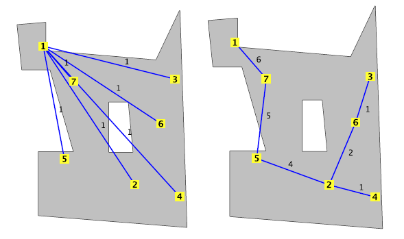
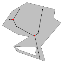
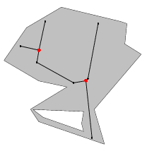
- 4.12
- In only 10 of the 100 cases, both methods found best networks with exactly the same topology. The location of Steiner points for those cases indicate that the geometric graph method finds better locations for the Steiner points. By definition, this leads to lower building costs. This is inherent in the way these methods define the location of a Steiner point. In the geometric graph method, a geometric algorithm is used to find within a subset of other nodes the optimal location for the Steiner point. In the agent-based model, an ant is attracted to network paths already built. When it finds the path, it will connect at that location. There is no extra optimization round to adjust the location of the connection point for two or more paths together. Figure 4.3 shows for one example the different ways in which Steiner points are found.
- 4.13
- Various other attempts to determine whether the topological differences resulting from the geometric graph method and the agent-based method explain the difference in building cost were inconclusive. This may be due to a lack of indicators for 'topological correspondence'.
- 4.14
- Overall, the topology of the best networks found by the
agent-based model and the geometric graph method differ slightly
with respect to the number and location of the Steiner points they
found: the geometric graph method finds more Steiner points and
locates them better. These differences can be expected to explain
the small difference in building costs to a large extent, although
it is hard to prove this conclusion statistically.
Computational performance
- 4.15
-
The results, as shown in figure 4.4 per individual run, indicate that
the method's speeds are competitive, but that the geometric graph
method is faster.
Table 4.5: Computational results of the experiments. (Only significant correlations ( α = 5%) are shown.) Correlation coefficient between time of one run and ... Parameter GGM ABM Total number of nodes N 0.74 0.24 Cost exponent β - -0.09 Maximum capacity demand of consumer nodes qmax - - Mean capacity demand of consumer nodes - - Length of minimal spanning tree connecting all nodes 0.59 0.24 Total variance of time explained adj. R2 55% 7.4%
Geometric graph method
- 4.16
-
The geometric graph method needs per run on average 8 seconds with
a standard deviation of 7 seconds, see figure 4.4. Furthermore, table 4.5 shows that the time per run has a
positive relation with the total number of nodes N to be connected and with the total length of
the minimal spanning tree lMST. Runs with random non-crossing
spanning trees as a starting point have a significantly lower speed
than runs starting from the star network or the minimal spanning
tree.
Agent-based modeling
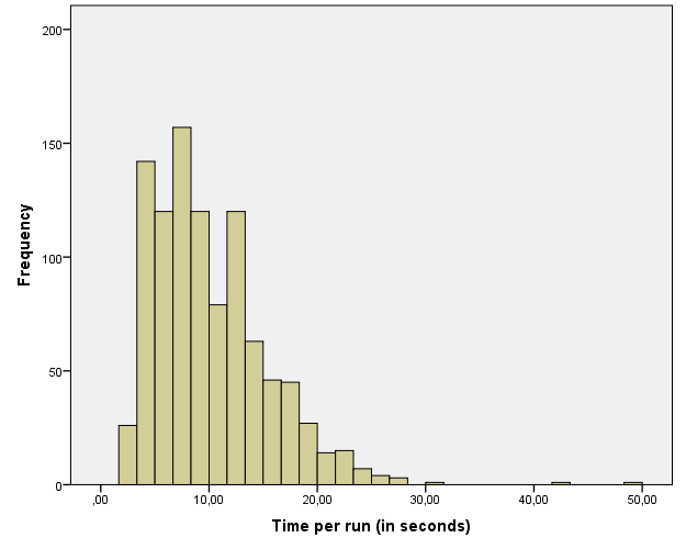
- 4.17
-
The agent-based method needs on average 10 seconds for one run,
with a standard deviation of 5 seconds for all runs, see figure
4.4. The distribution
differs from the geometric graph method ' it is more symmetric
around the average. This method shows more outliers (9 are not
shown). The model settings have a large impact on the speed.
Increasing population size, increasing patience or enabling more
pheromones slows the simulation down drastically. Table 4.4 shows that the time
needed for a run is hardly influenced by the problem
characteristics.
Figure 4.4: Time per run (in seconds) for 1000 (random) runs of both methods Geometric graph method
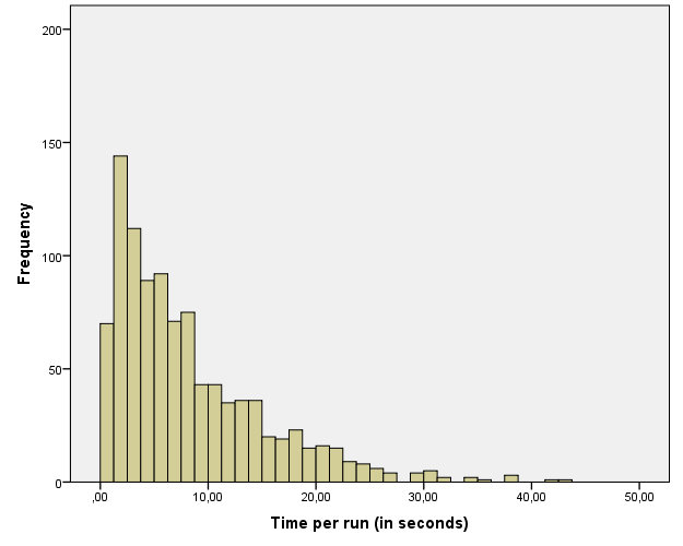
Agent-based model
Co-development of algorithms
- 4.18
- Developing the algorithms together proved useful for mutual
improvement of the approaches. Several improvements were made
during the process to both methods by comparing their behavior and
results.
Redirecting to shortest path
- 4.19
-
After each change of the network, the geometric graph method
redirects connections to the allowed region if necessary. If an
obstacle is part of this region, then multiple paths through the
region are possible. To find the best path, the allowed region is
triangulated using the ear-clipping method from (Eberly 1998). A connection passing a no-go area was
redirected to the path that had to pass the least number of
different triangles. However, triggered by some results of the
agent-based runs, it was clear that this path was not always the
shortest path to redirect edges. The algorithm was adapted in such
a way that not the path with the least number of triangles was
chosen, but the path with the shortest Euclidean length.
Starting network topology
- 4.20
-
Originally, the geometric graph method started from two extremes:
the minimal spanning tree and the star network. However, based on
the agent-based method, we recognized that more randomness might
lead to better solutions. Now, the method starts both from these
deterministic trees and from several random non-crossing spanning
trees to come to a good solution.
Network power
- 4.21
-
The agent-based approach was also inspired by developing both
approaches together. The main inspiration from the geometric graph
method is the role that the partially built network plays in the
simulation.
The network had to attract the ants, walking to the nest, in order to create Steiner points. Furthermore, this network
power now depends on β, the
relative costs of building larger capacity lines.
Strengths and weaknesses comparison
- 4.22
-
After having co-evolved the algorithms and comparing them
extensively, we have identified several strengths and weaknesses of
both approaches. These are presented in table 4.6.
Table 4.6: Features, strengths and weaknesses Aspect Geometric graph method Agent-based method Spatial representation Continuous graph, more precise Discrete patches, less precise Algorithm Complicated geometric heuristic Agents with simple decision making rules Optimality of solution Local optimum given by starting tree, slightly lower cost Local optimum given by order of connecting, slightly higher cost Feasible intermediate solutions Yes As soon as a path to all sources is found going through the allowed region Network topology and location Slightly more Steiner points, located better Slightly less Steiner points, located worse Computational time Fast, dependent on initial tree, few outliers Fast, dependent on model settings, more outliers Implementation Maple module NetLogo model Expandability Limited to geometric graph method Limited to agent decision rules and exogenous changes
Conclusions and future work
-
Conclusions
- 5.1
- This paper compares two approaches ' geometric graph method and
agent-based ACO ' for determining the optimal infrastructure
network layout in which one source needs to be connected to several
consumers at different capacities in closed 2D plane with an
obstacle. The geometric graph approach was adopted from (Heijnen et al.
2013) and a standard ant colony optimization was implemented as
an agent-based model. We have applied both approaches to 100 design
problems, in which the characteristics of the problem were varied.
Table 4.6 shows the main features of
the two approaches, which provide insight in the advantages and
disadvantages of using each of them.
- 5.2
- The geometric graph method slightly outperforms the agent-based method both in quality of the result as well in computational performance. The differences in performance are small and there are also optimization problems for which the agent-based method is the winner. At the end of the day, the two approaches are on par ' the quality and speed are acceptable for both. Each of the methods can be effectively used for a good-enough first layout of a tree-shaped infrastructure network. How good the approaches are in determining the optimal network layout depends on the network topologies that are found, the straightness of the network links, and the location of Steiner points. Both are effective in finding good topologies. The geometric graph method finds on average slightly more Steiner points and locates the Steiner points better. These differences can be expected to explain the difference in building costs to a large extent. Each of the methods can be expanded in different directions to cope with other planning uncertainties. Together they may prove to be valuable in real-world planning processes. The agent-based method is more easily applicable, as the NetLogo implementation is rather intuitive. Decision rules can be adapted to cope with other problem characteristics.
- 5.3
-
Both GGM and ABM use a heuristic approach and will in general result in a local optimum. However, finding an Edge-Weighted Steiner Minimal Tree is NP-hard (Thomas & Weng
(2006)) and an algorithm that can find the global optimum in polynomial time does not exist yet.
However, for small problems with just a few nodes to be connected and no closed region or obstacles, the optimum can be found by searching through all combinations of possible full Steiner trees. A full Steiner tree is a tree connecting k terminals using exactly k - 2 Steiner points. Heijnen et al.
(2013) performed 120 random experiments (equally distributed over N = 4, 5 and 6 nodes) to compare the final solution of the GGM to the optimum. In 110 out of the 120 experiments, i.e. 92%, the optimal solution was also found by the GGM. In all the other 10 cases, the costs of the proposed network exceeded the minimal costs by less than 1%.
In practice, however, not optimal network planning algorithms but common sense and expert judgment is used to find a good network layout. It might therefore be more useful to investigate whether the proposed methods would perform better than these conventional methods. Unfortunately, sufficient evidence for this hypothesis is hard to find.
We propose that the resulting networks from GGM or ABM could serve as promising initial layouts open for discussion and adaptation due to overwhelming specific local details that can never be accommodated for in algorithms.
Future work
- 5.4
-
A number of development directions are conceivable, namely
connecting multiple sources to multiple sinks, cost differentiation in network region, participation probability and cost for splitting and corners points. These
will be described below.
Connecting multiple sources
- 5.5
- New networks might also be fed by multiple sources, instead of one, or nodes could even be both supplier and consumer of the network on different moments in time. In these cases, it might be profitable to build a network that has multiple paths between two nodes. In that case the network no longer has a tree topology.
- 5.6
- The geometric graph method uses a mathematical criterion to determine whether or not it is profitable to combine some connections partly and split them on another location. The optimal location of the splitting point is exactly determined by a geometric technique. If the network is no longer a tree, these methods can still be used but they might become more complicated when β, the cost exponent for the capacity, is large.
- 5.7
-
In the agent-based method, other ant nests can easily be added
and the nest scent on a patch would be the sum of the scent from
both nests. Minor changes to the decisions of the ants are needed
in this case.
Cost differentiation in networks
- 5.8
-
The region is currently divided in an allowed part and a no-go
area. In specific cases, it might however be possible to construct
a connection passing no-go areas, but at some expense. For
instance, highways, canals, or other obstacles could be considered.
Similarly, stretches with existing infrastructure could be made
cheaper. Constructing pipelines next to existing infrastructure
generally is cheaper because one can share permits, ownership and
preparation of soil and land.
- 5.9
- The geometric graph method needs to find, instead of a shortest
path through an allowed region, a cheapest path between two points.
There are approximation algorithms for this problem, however
determining the exact cheapest path is an unsolvable problem
(Carufel et al. 2014) The agent-based method currently defines the no-go area as an
extremely costly area. It is straightforward to differentiate these
costs and, accordingly, to make it more attractive to choose a
shorter path through a more expensive area, than to choose a longer
path through a cheaper area.
Probability of sources to participate
- 5.10
- A particular challenge of network planning is the multi-actor
context. It is not always certain who will participate.
For both methods a similar approach may be followed, i.e. the
approach that (Heijnen et al. 2013) used for the geographic graph
method. Resulting networks are recorded from many simulation runs
in which the set of consumer nodes that are considered is varied,
according to the estimated probability of taking part. One approach
to analyze these results is to make an overlay of all the resulting
networks and look at a density (or probability) plot of network
pipelines built in the region.
Costs for splitting and corners
- 5.11
- Part of the costs for a network is determined by the corners and splitting points and they could be accounted for in determining the cheapest cost network. The geometric graph method could account in the calculation of the network cost. In that case, an extra comparison needs to be made between network cost for adding a Steiner point to connect a subset of nodes to network costs using the minimal spanning subtree to connect the same subset. This willx need a small adaptation of the current procedure. In the agent-based method splitting points and corners, accounting for costs for splitting and corners only requires to include those in the calculation of network cost.
Acknowledgements
- The authors acknowledge the work of MSc students Guy Rutten and András Kóváry in creating the initial NetLogo ACO implementation as a part of their course work for SPM9555, Advanced Agent Based Modeling course at the SEPAM programme at the Faculty of Technology, Policy and Management of the Delft University of Technology, the Netherlands.
References
-
ALTIPARMAK, F. &
KARAOGLAN, I. (2007).
A genetic ant colony optimization approach for concave cost
transportation problems.
In: Evolutionary Computation, 2007. CEC 2007.
IEEE Congress on. IEEE. [doi:10.1109/cec.2007.4424676]
ARNAOUT, J.-P. (2013). Ant colony optimization algorithm for the euclidean location-allocation problem with unknown number of facilities. Journal of Intelligent Manufacturing 24(1), 45-54. [doi:10.1007/s10845-011-0536-2]
BIJKER, W., HUGHES, T. & PINCH, T. (1987). The Social construction of technological systems : new directions in the sociology and history of technology. MIT Press. Cambridge, Mass.
BORSHCHEV, A. & FILIPPOV, A. (2004). From system dynamics and discrete event to practical agent based modeling: Reasons, techniques, tools. In: The 22nd International Conference of the System Dynamics Society. Oxford, England. http://www.econ.iastate.edu/tesfatsi/systemdyndiscreteeventabmcompared.borshchevfilippov04.pdf.
CARUFEL, J. L. D., GRIMM, C., MAHESHWARI, A., OWEN, M. & SMID, M. (2014). A note on the unsolvability of the weighted region shortest path problem. Computational Geometry 47(7), 724-727. [doi:10.1016/j.comgeo.2014.02.004]
CHANDRA MOHAN, B. & BASKARAN, R. (2012). A survey: Ant colony optimization based recent research and implementation on several engineering domain. Expert Systems with Applications 39(4), 4618-4627. [doi:10.1016/j.eswa.2011.09.076]
CHAPPIN, E. J. L. (2011). Simulating Energy Transitions. Ph.D. thesis, Delft University of Technology, Delft, the Netherlands. http://chappin.com/ChappinEJL-PhDthesis.pdf. ISBN: 978-90-79787-30-2.
DIXIT, A. K. & PINDYCK, R. S. (1994). Investment under uncertainty. Princeton, N. J.: Princeton University Press. ISBN 0691034109.
DORIGO, M. & DI CARO, G. (1999). Ant colony optimization: a new meta-heuristic. In: Evolutionary Computation, 1999. CEC 99. Proceedings of the 1999 Congress on, vol. 2. IEEE. [doi:10.1109/cec.1999.782657]
DORIGO, M., MANIEZZO, V. & COLORNI, A. (1996). Ant system: optimization by a colony of cooperating agents. Systems, Man, and Cybernetics, Part B: Cybernetics, IEEE Transactions on 26(1), 29-41. [doi:10.1109/3477.484436]
EBERLY, D. (1998). Triangulation by ear clipping. http://www.geometrictools.com/.
EPSTEIN, J. M. & AXTELL, R. (1996). Growing artificial societies: social science from the bottom up. Complex adaptive systems. Washington, D.C.: Brookings Institution Press; MIT Press.
GASTNER, M. T. & NEWMAN, M. E. (2006). Shape and efficiency in spatial distribution networks. Journal of Statistical Mechanics: Theory and Experiment 2006(01), P01015. [doi:10.1088/1742-5468/2006/01/p01015]
GEEM, Z. W. (2009). Particle-swarm harmony search for water network design. Engineering Optimization 41(4), 297-311. [doi:10.1080/03052150802449227]
HEIJNEN, P. W., LIGTVOET, A., STIKKELMAN, R. M. & HERDER, P. M. (2013). Maximising the worth of nascent networks. Networks and Spatial Economics 14(1), 27-46. [doi:10.1007/s11067-013-9199-1]
HU, Y., JING, T., FENG, Z., HONG, X.-L., HU, X.-D. & YAN, G.-Y. (2006). Aco-steiner: ant colony optimization based rectilinear steiner minimal tree algorithm. Journal of Computer Science and Technology 21(1), 147-152. [doi:10.1007/s11390-006-0147-0]
HWANG, F. & RICHARDS, D. S. (1992). Steiner tree problems. Networks 22(1), 55-89. [doi:10.1002/net.3230220105]
IPCC (2007). Climate Change 2007: Mitigation of Climate Change Summary for Policymakers. Geneva: IPCC.
KABIRIAN, A. & HEMMATI, M. R. (2007). A strategic planning model for natural gas transmission networks. Energy policy 35(11), 5656-5670. [doi:10.1016/j.enpol.2007.05.022]
LEE, D. & PREPARATA, F. (1984). Euclidean shortest paths in the presence of rectilinear barriers. Networks 14, 393-410. [doi:10.1002/net.3230140304]
LIU, Q. & WANG, C. (2012). Multi-terminal pipe routing by steiner minimal tree and particle swarm optimisation. Enterprise Information Systems 6(3), 315-327. [doi:10.1080/17517575.2011.594910]
MAIER, H. R., SIMPSON, A. R., ZECCHIN, A. C., FOONG, W. K., PHANG, K. Y., SEAH, H. Y. & TAN, C. L. (2003). Ant colony optimization for design of water distribution systems. Journal of water resources planning and management 129(3), 200-209. [doi:10.1061/(ASCE)0733-9496(2003)129:3(200)]
MARCOULAKI, E. C., PAPAZOGLOU, I. A. & PIXOPOULOU, N. (2012). Integrated framework for the design of pipeline systems using stochastic optimisation and gis tools. Chemical Engineering Research and Design . [doi:10.1016/j.cherd.2012.05.012]
MIDDLETON, R. S. & BIELICKI, J. M. (2009). A scalable infrastructure model for carbon capture and storage: Simccs. Energy Policy 37(3), 1052-1060. [doi:10.1016/j.enpol.2008.09.049]
PARK, J.-H. & STORCH, R. L. (2002). Pipe-routing algorithm development: case study of a ship engine room design. Expert Systems with Applications 23(3), 299-309. [doi:10.1016/S0957-4174(02)00049-0]
PISANSKI, T. (2000). Bridges between geometry and graph theory. In: in Geometry at Work, C.A. Gorini, ed., MAA Notes 53. America.
QIN, Y., QIN, L. & LI, H. (2012). Study on route optimization of logistics distribution based on ant colony and genetic algorithm. In: Instrumentation & Measurement, Sensor Network and Automation (IMSNA), 2012 International Symposium on, vol. 1. IEEE. [doi:10.1109/msna.2012.6324569]
SAMMUT, C. & WEBB, G. I. (2011). Encyclopedia of machine learning. Springer-Verlag New York Incorporated.
THOMAS, D. & WENG, J. (2006). Minimum cost flow-dependent communication networks. Networks 48(1), 39-46. [doi:10.1002/net.20118]
VIEBAHN, P., ESKEN, A. & FISCHEDICK, M. (2009). Energy-economic and structural, and industrial policy analysis of re-fitting fossil fired power plants with co2 capture in north rhine-westphalia/germany. Energy Procedia 1, 4023-4030. [doi:10.1016/j.egypro.2009.02.208]
WU, P.-C., GAO, J.-R. & WANG, T.-C. (2007). A fast and stable algorithm for obstacle-avoiding rectilinear steiner minimal tree construction. In: Proceedings of the 2007 Asia and South Pacific Design Automation Conference. IEEE Computer Society. [doi:10.1109/ASPDAC.2007.357996]