
 Abstract
- Models of social systems generally contain free parameters that cannot be evaluated directly from data. A calibration phase is therefore necessary to assess the capacity of the model to produce the expected dynamics. However, despite the high computational cost of this calibration it doesn't produce a global picture of the relationship between the parameter space and the behaviour space of the model. The Calibration Profile (CP) algorithm is an innovative method extending the concept of automated calibration processes. It computes a profile that depicts the effect of each single parameter on the model behaviour, independently from the others. A 2-dimensional graph is thus produced exposing the impact of the parameter under study on the capacity of the model to produce expected dynamics. The first part of this paper is devoted to the formal description of the CP algorithm. In the second part,we apply it to an agent based geographical model (SimpopLocal). The analysis of the results brings to light novel insights on the model.
- Keywords:
- Calibration Profile, Model Evaluation
Introduction
- 1.1
- Agent-based modelling is widely used in models of social systems because it is well suited to describe individual-centred dynamics with non-linear interactions. This modelling technique, however, introduces many free parameters which critically influence the behaviour of the model. Hand-picking parameters is a time-consuming process and makes it hard to evaluate the ability of a model to reproduce empirical data or formalised knowledge. Automatic calibration of models have the potential to free the modeller from this burden and to make the modelling process more rigorous by reducing the number of arbitrary choices.
- 1.2
- The current prevalent method for automatic calibration is to see it as an optimisation problem in which the differences between known data and model predictions have to be minimised. This optimisation can be performed with different optimisation algorithms like "Approximate Bayesian Computation" (Lenormand et al. 2012) or evolutionary algorithms (Schmitt et al. 2014; Stonedahl 2011). Nevertheless, these methods find a single set of parameters, or, in the case of multi-objective evolutionary algorithms, several sets of parameters that represent optimal trade-off with regard to several model quality criteria. In both cases, the result of the calibration is solely that the model can reproduce the data with a given precision. These calibration processes do not say anything about how often parameter sets lead to realistic behaviours, and about how each parameter changes the behaviour of the model. For instance, it is often interesting to know when some parameter values would prevent the system to reach a realistic behaviour, rather than only knowing a single set of "optimal" parameter values.
- 1.3
- To compute a more global view of the parameter space, we have designed a novel method that exposes the sensitivity of a single parameter on the calibration of a model independently of the other parameters. A high level representation of this method is shown on Figure 1. It computes the lowest calibration error that can possibly be obtained when the value of a given parameter is fixed and the others are free. It computes this minimal error for many values of the parameter under study. The values of the parameter are sampled all along its domain of definition to produce a so called calibration profile. For each sample value, the value of the remaining parameters are optimised in order to find the lowest possible calibration error. The profile can then be drawn on a 2-dimensional chart that depicts the influence of the parameter under study on the model calibration.
- 1.4
- Conceptually, CP are similar to likelihood profiles (Pawitan 2001), a classic tool
in statistics[1].
However, computing likehood profiles requires an analytical expression
of the model, which is infortunately not available in most agent-based
simulations, whereas calibration profiles can be used with any model. A
calibration profile can thus be seen as a way to approximate the
likelihood profile when the analytical expression of the model is not
available or is too complicated.
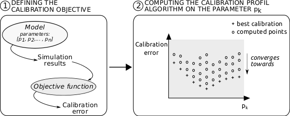
Figure 1. High level representation of the Calibration Profile (CP) method - 1.5
- To produce a calibration profile, a naive approach would consist in executing an entire calibration algorithm for each value of the parameter under study. Current automated calibration algorithms are too computationally intensive to make this approach tractable in practice. To tackle this problem we have designed an algorithm that computes the numerous points composing a calibration profile altogether. The design of this algorithm has been inspired by the recently published MOLE method (Clune et al. 2013; Mouret & Clune 2012), which pictures 2-dimensional phenotype landscapes for evolutionary biology. MOLE and the CP method are both stochastic, population-based search algorithms that exploit the fact that a small change to a good solution is likely to lead to another similarly good solution (Deb et al. 2002). Nonetheless, while classic stochastic optimization algorithms search for a single optimum of a function, the CP method aims to fill a 1-dimensional array of "categories" (a 2-D map for MOLE) that should each contain the best performing sample for each possible value of the parameter under scrutinity (after a discretization). To do so, the algorithm starts by generating a a few random samples, evaluates their performance, and stores the best sample of each category; these best samples are then randomly modified to generate new samples, thus having a chance to either improve the best samples of the current categories, of fill new categories in the neighborhood with high-peforming samples.
- 1.6
- The first section of this paper exposes a formal description of the CP algorithm as well as a reusable implementation of the method. In the second section we show how the application of the CP algorithm to a real world geographical simulation model produces novel insights toward the validation of the model.
The
Calibration Profile (CP) algorithm
-
Intuition
- 2.1
- To compute the calibration profiles we propose a new
algorithm designed in the framework of evolutionary algorithms. Figure 2 illustrates the
progress of this algorithm through the example of the computation of a
9 points profile along x1 of a function f(x1, x2). In this example, the
function f computes the evaluation of a 2-parameter model (x1 and x2).
The calibration objective is to minimise f(x1, x2). In the step 1 the
algorithm randomly samples points (random values of x1 and x2) and
computes f(x1, x2). In the step 2, the algorithm divides the definition
domain of x1 in 9 disjoint even intervals and keeps only the sampled
point with the lowest f(x1, x2) in each of these intervals (this
constitutes the elitism stage). The points that have been selected
constitute a first approximation of the calibration profile of the
model f along x1. In step 3 new samples (x1, x2) are generated by
mutating the points in the current approximation of the calibration
profile and f(x1, x2) is evaluated for each of these new points. The
newly evaluated samples are merged with the existing ones and the
algorithm iterates to the step 2. This iteration stops once a given
stopping criterion is met after step 2. The projection of the last
selected points along x1 constitutes an approximation of the
theoretical continuous profile (step 4).
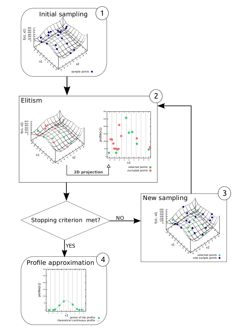
Figure 2. Intuition of the profile algorithm. Objective
- 2.2
- The CP method takes inspiration from evolutionary algorithms to provide a thorough analysis of the role played by each parameter. Such analysis is independent from one parameter to the other. A function that evaluates the performance of each particular model is supposed to be given (typically such evaluation takes into account the fitting of the model to the data).
- 2.3
- Let
 be the set of possible models under
consideration and let
A
= A1×…×An⊆
be the set of possible models under
consideration and let
A
= A1×…×An⊆ n be the domain of the
parameter vectors that we consider as determining the models, where n
is the number of parameters. We denote by
n be the domain of the
parameter vectors that we consider as determining the models, where n
is the number of parameters. We denote by
 the map that provides a
model for a given
parameter vector. Such map can be viewed as a meta-model, that is a
model with free parameters.
the map that provides a
model for a given
parameter vector. Such map can be viewed as a meta-model, that is a
model with free parameters.
- 2.4
- Let
 be the function providing an evaluation for each
model. We can obviously evaluate a parameter vector with the function
be the function providing an evaluation for each
model. We can obviously evaluate a parameter vector with the function
 . In this context, when we
use the word solution
we just mean a parameter vector
. In this context, when we
use the word solution
we just mean a parameter vector
 ∈A.
By convention we suppose that best solutions are closer to 0.
∈A.
By convention we suppose that best solutions are closer to 0.
- 2.5
- To estimate the impact of the k-th
parameter on the model, we consider the function
hk
: Ak→
defined by
hk(x) = inf{f (a1…, ak-1, x, ak+1,…, an) : aj∈Aj}. - 2.6
- This function produces, for a fixed value of the k-th parameter (i.e. ak = x), the best possible performance of the model. In our view, this function is a good indicator of the impact of a parameter and provides valuable information for further analysis.
- 2.7
- Our aim is then to compute, for each
k∈{1,…,
n}, a good approximation of hk.
A naive approach would consist in sampling Ak,
say by choosing
{a1k,…,
alkk}⊂Ak,
and running one optimisation algorithm for each ajk
to approximate hk(ajk).
Unfortunately this method is very inefficient. To overcome the
computational limits of this approach, we propose a new algorithm that
converges directly to the whole set
{hk(a1k),…,
hk(alkk)}.
Description of the algorithm
- 2.8
- In this section we consider k∈{1,…, n} to be fixed and we describe the CP algorithm for the analysis of the k-th parameter. As mentioned earlier, the goal is to approximate hk(x), that is to provide sufficiently good approximations of hk(ajk), for certain a1k,…, alkk∈Ak.
- 2.9
- In order to explore Ak
uniformly, we use an evolutionary algorithm with diversity pressure
mechanism (Goldberg et al. 1992;
Toffolo & Benini 2003;
Mahfoud 1997; Mouret & Doncieux 2012).
Let C1,…,
Clk
be lk different semantic
categories to which one can associate an element belonging to Ak.
In our approach, we consider that categories can be identified with
intervals
I1,…,
Ilk⊆Ak,
and that such intervals form a partition of Ak:
- Ii∩Ij = ∅ if i≠j, and
 .
.
- 2.10
- We assume that these categories are good enough to
characterise Ak, that is
they are a good discretisation of Ak.
For each ak∈Ak,
we denote by cat(ak)
the category of ak, that is
the unique category Cj such
that ak∈Ij.
We also denote by
Cat
: A→{C1,…,
Clk}
the map defined by Cat() = cat(ak),
where
 ; it defines the category of a parameter vector
as the category of its k-th coordinate. The
algorithm is devised to find parameter vectors
{
; it defines the category of a parameter vector
as the category of its k-th coordinate. The
algorithm is devised to find parameter vectors
{ ,…,
,…, },
with
},
with  and aji∈Ai,
such that:
and aji∈Ai,
such that:
- Each vector lies in a different category:
Cat(
 )
= Cj
for j =
1…lk. This means that, when
projecting on the k>-th coordinate, our
sample is representative of the whole space Ak.
)
= Cj
for j =
1…lk. This means that, when
projecting on the k>-th coordinate, our
sample is representative of the whole space Ak.
- For each ,
the value of f
() is a good approximation
of hk().
- Each vector lies in a different category:
Cat(
- 2.11
- The idea of the algorithm is to generate successive sets of
solutions and to keep only the best solution per category. At each
iteration the set of best solutions is updated.
The algorithm is composed of the following steps:
We first generate a random set X0 of parameter vectors, that is X0 = {,…, },
with = (aj1,…,
ajn)
and aji∈Ai.
},
with = (aj1,…,
ajn)
and aji∈Ai.
We can consider, by induction, that XN has already been constructed at this point.Let us define the sets Si = {
Check if a predefined stopping criterion is met (number of iterations, stabilisation of the solutions, etc.). Go to Step 4 if it is, continue to Steps 3 if it is not. Generate H* from H by randomly modifying the parameter vectors in H. We can for instance generate each vector in H* by applying a gaussian variation to a vector in H. Define the set XN+1 as the union of H and H* and go to Step 2. When the stopping criterion is met, we can output our approximation to the function hk(x): If {∈XN
: Cat() = Ci}
for i
= 1,…, lk (we may get
Si
= ∅ for some values of i). Then we apply elitism,
that is we select only the best parameter vector in each category: We
define the sets
Ei
= {∈Si
: f ()≤f ( )
∀∈Si}
for i
= 1,…, lk, and
)
∀∈Si}
for i
= 1,…, lk, and
 . In practice all the sets Ei
will be either empty, if Si
= ∅, or containing only one element (if
|Ei|≥2
we can randomly choose one element in Ei
and consider Ei composed of
just that element). ,…,
. In practice all the sets Ei
will be either empty, if Si
= ∅, or containing only one element (if
|Ei|≥2
we can randomly choose one element in Ei
and consider Ei composed of
just that element). ,…, }
is the last H computed, our approximation to hk(x)
is the set of 2-tuples
{(
}
is the last H computed, our approximation to hk(x)
is the set of 2-tuples
{( ,
f ()),…,(
,
f ()),…,( ,
f ())}. Let us note that
m≤lk
by construction, but in practice, when the number of iterations is high
enough (see section 2.1
point 1)
we get m = lk.
,
f ())}. Let us note that
m≤lk
by construction, but in practice, when the number of iterations is high
enough (see section 2.1
point 1)
we get m = lk.
Validity
- 2.12
- As we said in paragraph 2.7,
our approach consists in estimating the impact of the k-th
parameter on the performance of the model, by finding a good
approximation to the function hk(x).
To clarify why our method provides indeed such a good approximation, we
make the following remarks:
- At each iteration we randomly generate new solutions
from old ones. Given a solution such that that Cat() = Cj,
the probability of getting a new solution from such that Cat()
= Cj', with j'≠j,
is different from 0 (this is clearly the case if we use, for instance,
a gaussian variation). Hence, if enough iterations are repeated, every
category will eventually be reached by as many solutions as we wish.
- Let us consider u = inf{f
()
: Cat() = Cj}
= inf{hk(a)
: cat(a) = Cj}.
If the f is sufficiently regular (it is enough if
it is continuous, or if it is just semi-continuous on its local
minima), then, by the analogous argument to that in point 1., we will
eventually find an solution such that Cat() = Cj
and f () is as close to u
as we want.
- At each iteration we randomly generate new solutions
from old ones. Given a solution
- 2.13
- These remarks, together with the fact that we can consider
as many categories as needed, justify our claim. We should note that,
as it is usually the case with evolutionary algorithms, we do not
provide a precise speed of convergence for our algorithm; however,
experimental results are very satisfactory (see section 3).
Heuristic improvement
- 2.14
- In paragraph 2.11 we have presented the most basic version of our algorithm, for the sake of clarity. However in practice we use a variation of it, heuristically devised, to improve its performance. In this section we present these modifications. We use the same notation as in paragraph 2.11.
- 2.15
- The main point of this modified version is the random generation of new solutions (step 3). In this part we rely on the standard techniques used in genetic algorithms, in which the random variation comes from two biologically-inspired operators: mutation and crossover. These operators are not applied to the whole set H of solutions, but rather on a subset H0⊆H which is generated by a certain selection mechanism (we will explain below this selection mechanism). From H0 we generate H* in two steps: We first generate a new set of solutions H'0 by applying a SBX-crossover to H0 (see Deb & Agrawal 1994), and then we apply a self-adapting Gaussian mutation to H'0 (see Hinterding 1995). The result is our H*.
- 2.16
- In the selection of
H0⊆H
we follow a standard selection mechanism: Binary tournament selection.
It consists in randomly choosing two solutions
x,
y∈H, comparing them via a
certain function
g
: H→∪{∞}
and then keeping the best (x is kept if
g(x)≥g(y));
we repeat this procedure until we reach the desired size of H0.
Note Although we have defined H0 as a set (elements in H0 are unique), we can also define H0 as a tuple, allowing a same solution to appear more than once.
- 2.17
- One feature that is specific to our approach is the
definition of the function g, that we call local
contribution.
Definition Let H = {,…,}
and
 . Given a solution
∈H
. Given a solution
∈H  {,},
let Δj denote the area of
the triangle in 2
formed by the 2-tuples (
{,},
let Δj denote the area of
the triangle in 2
formed by the 2-tuples ( , f (
, f ( )),
(
)),
( ,
f ())
and (
,
f ())
and ( ,
f (
,
f ( )).
Then we define the local contribution of , as
g(
)).
Then we define the local contribution of , as
g( )
= (- 1)eΔj,
where e = 0 if the point (, f ()) is below the straight
line from (, f ()) and (,
f ()),
and e = 1 if it is not. If
is extreme, i.e. ∈{,},
then we define g()
= ∞.
)
= (- 1)eΔj,
where e = 0 if the point (, f ()) is below the straight
line from (, f ()) and (,
f ()),
and e = 1 if it is not. If
is extreme, i.e. ∈{,},
then we define g()
= ∞.
- 2.18
- We have just described how to generate a new set of solutions H* from H. The heuristics behind this procedure is to give some priority to the generation of new solutions that are either locally good, which accelerates the approximation to the local minima in each category, or on the extremes, which widens the exploration of the space.
- 2.19
- In order to describe the version of the algorithm that we use in the experiments, the other point we should mention is the stopping criterion. A natural choice would be based on the stability of the successive H computed: If we detect no important changes from one H to the next one (during several iterations), the algorithm stops. We can measure these changes in different ways, for instance considering the function F(H) =
 f
().
However, in practice, we consider a maximal computation time as the
stopping criterion and the stability becomes an element of subsequent
analysis.
f
().
However, in practice, we consider a maximal computation time as the
stopping criterion and the stability becomes an element of subsequent
analysis.
Generic implementation
- 2.20
- In order to make the CP algorithm usable we provide along with this paper a generic implementation in the free and open source library called MGO (Multi Goal Optimisation)[2] programmed in Scala[3]. MGO is a flexible library of evolutionary algorithms. It leverages the Scala "trait" system to provide a high level of modularity.
- 2.21
- This section shows how to compute a calibration profile on a toy model with MGO. In this example, the model is the Rastrigin function and the objective is to minimise this function. The objective function in MGO should be implemented through a specialised trait of the "Problem" trait. Listing 1 shows how to implement the Rastrigin function into MGO.
Listing 1. Implementation of the Rastrigin function in MGO.
import fr.iscpif.mgo._
import math._
import ultil.Random

trait Rastrigin <: GAProblem with MGFitness {
 def min = Seq.fill(genomeSize)(-5.12)
 def max = Seq.fill(genomeSize)(5.12)

 type P = Double

 def express(genome: Seq[Double], rng: Random) =
 10 * x.size + x.map(x => (x * x) - 10 * cos(2 * math.Pi * x)).sum

 def evaluate(phenotype: P, rng: Random) = Seq(phenotype)
}- 2.22
- To compute a calibration profile of this Rastrigin function it should be composed with the "Profile" trait that provides the CP algorithm. Listing 2 shows how to achieve this composition. In this example two other traits are used: A termination criterion based on a maximum number of steps ("CounterTermination") and a trait to specify that the profile is computed on a part of the genome ("ProfileGenomePlotter").
Listing 2. Computing the profile of the Rastrigin function in MGO.
import fr.iscpif.mgo._
import scalax.io._

object TestProfile extends App {
 val profile = new Rastrigin
 with Profile
 with CounterTermination
 with ProfileGenomePlotter {
 def genomeSize: Int = 6
 def lambda: Int = 200
 def steps = 200
 def x: Int = 0
 def nX: Int = 1000
 }

 implicit val rng = newRNG(42)

 val res =
 m.evolve.untilConverged {s =>
 println(s.generation)
 }.population

 val output = Resource.fromFile("/tmp/profile.csv")
 for {
 i <- res.toIndividuals
 x = m.plot(i)
 v = m.aggregate(i.fitness)
 if !v.isPosInfinity
 } output.append(s"$x,$v\n")
}- 2.23
- Like most evolutionary algorithms, the CP algorithm compute the evaluation function many times. Those numerous evaluations could be computationally costly. To cope with this, MGO takes advantages of the multi-core parallelism avaiable in modern computers. This kind of parallelism is suitable for many models but can be limiting in case of large stochastic agent based models for instance. To overpass this limit we have integrated the CP algorithm in the OpenMOLE[4] (Open Model Exploration) framework (Reuillon et al. 2013). OpenMOLE enables the distribution of the CP algorithm on large scale distributed computing infrastructures including multi-core computers, computing clusters and even world wide computational grids. In the following section we used this distributed implementation of CP framework to study a real world agent based model.
Application the SimpopLocal geographical
model
-
A model to simulate the emergence of structured urban settlement system
- 3.1
- SimpopLocal is a stylised model of an agrarian society in
the Neolithic period, during the primary “urban transition” manifested
by the appearance of the first cities (Schmitt
et al. 2014). It is designed to study the emergence
of a structured and hierarchical urban settlement system by simulating
the growth dynamics of a system of settlements whose development
remains hampered by strong environmental constraints that are
progressively overcome by successive innovations. This exploratory
model seeks to reproduce a particular structure of the Rank-Size
distribution of settlements well defined in the literature as a
generalised stylised-fact: For any given settlement system throughout
time and continents, the distribution of sizes is strongly
differentiated, exhibiting a very large number of small settlements and
a much smaller number of large settlements (Liu
1996; Durand-Dastès
et al. 1998; Berry
1964; Fletcher 1986).
This kind of distributions can be modeled by a power-law when small
settlements are not considered or a log-normal when small settlements
are considered (Robson 1973;
Favaro & Pumain 2011).
Such distributions are easily simulated by rather simple and non
spatial statistical stochastic models (Gibrat
1931; Simon 1955).
But for theoretical considerations and to specify the model in a
variety of geographical frames, we think it is necessary to make
explicit
the spatial interaction processes that generate the evolution of city
systems. According to the evolutionary theory of system of cities (Pumain 1997, 2009), the growth dynamics of
each settlement is controlled by its ability to generate interurban
interactions. The multi-agent system modeling framework enables us to
include mechanisms, derived from this theory, that govern the
interactions between settlements (Bretagnolle
et al. 2006; Pumain
& Sanders 2013). The application of this concept
resulted in several Simpop models (Bura
et al. 1996; Bretagnolle
& Pumain 2010; Sanders
et al. 1997) in which the expected macro-structure
of the log-normal distribution of sizes emerges from the differentiated
settlement growth dynamics induced by the heterogeneous ability of
interurban interactions. Therefore the aim of SimpopLocal is to
simulate the hierarchy process via the explicit modelling of a growth
distribution that is not entirely stochastic as in the Gibrat model (Gibrat 1931) but that emerges
from the spatial interactions between micro-level entities.
Agents, attributes, and mechanisms of the model
- 3.2
- The SimpopLocal model is a multi-agent model developed with
the Scala software programming language. The landscape of the
simulation space is composed of a hundred of settlements. Each
settlement is considered as a fixed agent and is described by three
attributes: The location of its permanent habitat, the size of its
population, and the available resources in its local environment. The
amount of available resources is quantified in units of inhabitants and
can be understood as the carrying capacity of the local environment for
sustaining a population. This carrying capacity depends on the
resources exploitation skills that the local population has acquired
from inventing or acquiring innovation. Each new innovation acquired by
a settlement develops its exploitation skills. This resource
exploitation is done locally and sharing or trade is not explicitly
represented in the model. The growth dynamics of a settlement is
modelled according to the assumption that its population size is
dependent on the amount of available resources in the local environment
and is inspired from the Verhulst model (Verhulst
1845) or logistic growth. For this experiment, we assume a
continuous general growth trend for population - this may be different
in another application of the model. The annual growth factor rgrowth
is expressed on an annual basis, thus one iteration or step of the
model simulates one year of demographic growth. rgrowth
has been empirically estimated to 0.02. The limiting factor of growth RMi
is the amount of available resource that depends on the number M
of innovations the settlement i has acquired by the
end of the simulation step t. Pti
is the population of the settlement i at the
simulation step t:
Pt+1i = Pti.[1 + rgrowth.(1 -  )]
)]
- 3.3
- The acquisition of a new innovation by a settlement allows
it to overtake its previous growth limitation by allowing a more
efficient extraction of resources and thus a gain in population size
sustainability. With the acquisition of innovations the amount of
available resources tends to the maximal carrying capacity Rmax
of the simulation environment:
RMi  Rmax
Rmax
- 3.4
- The mechanism of this impact follows the Ricardo model of
diminishing returns, also a logistic model (Turchin
2003). The InnovationImpact parameter
represents the impact of the acquisition of an innovation and has a
decreasing effect on the amount of available resources RMi
with the acquisition of innovations:
RM+1i = RMi.[1 + InnovationImpact.(1 -  )]
)]
- 3.5
- Acquisition of innovations can occur in two ways, either by
the emergence of innovation within a settlement or by its diffusion
through the settlement system. In both cases, interaction between
people inside a settlement or between settlements is the driving force
of the dynamics of the settlement system. It is a probabilistic
mechanism, depending on the size of the settlement. Indeed, innovation
scales super-linearly: The greater the number of innovations acquired,
the bigger the settlement and the higher the probability of innovating (Lane et al. 2009; Diamond 1997). To model the
super-linearity of the emergence of innovation within a settlement, we
model its probability by a binomial law. If Pcreation
is the probability that the interaction between two individuals of a
same settlement is fruitful, i.e. leads to the creation of an
innovation, and N the number of possible
interactions, then by the binomial law, the probability Π
of the emergence of mcreation innovations can be
calculated. It is thus possible to compute the probability Π(mcreation
> 0) that at least one innovation appears in a given
settlement i. This probability then can be
used in a random
drawing:
Π(mcreation > 0) = 1 - Pm=0 Π(mcreation > 0) = 1 - [  .Pcreation0.(1
- Pcreation)N-0]
.Pcreation0.(1
- Pcreation)N-0]
Π(mcreation > 0) = 1 - (1 - Pcreation)N - 3.6
- If the size of the settlement i
considered is Pti
then the number N of possible pairwise interactions
between
individuals of that settlement is:
- 3.7
- The diffusion of an innovation between two settlements
depends both on the size of populations and the distance between them.
If Pdiffusion is the
probability that the interaction of two individuals of two different
settlements is fruitful, i.e. leads to the transmission of the
innovation, and K the number of possible
interactions, then by the Binomial law the probability Π
of the diffussion of mdiffusion innovations can
be calculated. It is thus possible to compute the probability Π(mdiffusion
> 0) that at least one innovation appears in a given
settlement i. This probability then can
be used in a random
drawing:
Πmdiffusion > 0 = 1 - (1 - Pdiffusion)K - 3.8
- But in this case, the size K of the
total population interacting is a fraction of the population of the two
settlements i and j which is
decreasing by a factor DistanceDecay with the
distance Dij between the
settlements, as in the gravity model (Wilson
1971):
- 3.9
- However another mechanism controls this innovation diffusion process. Each innovation can only be diffused during a time lap just after its acquisition by a settlement. This time lap of diffusion is controlled by the parameter InnovationLife. According to this deprecation mechanism, an innovation is considered obsolete after InnovationLife simulated years and cannot be diffused any more.
- 3.10
- SimpopLocal involves six free parameters that cannot be
evaluated using empirical values: InnovationLife, InnovationImpact,
Rmax, Pcreation,
Pdiffusion, DistanceDecay.
Those parameters are constrained by the definition domains shown in
Table 1.
Table 1: Definition boundaries for SimpopLocal parameters Parameter Definition domain Rmax [1;40,000] InnovationImpact [0;2] Pcreation [0;0.1] Pdiffusion [0;0.1] DistanceDecay [0;4] - 3.11
- In order to ensure the replicability of the model, a
portable implementation has been designed and the source code of
SimpopLocal used in this experiment has been filed in a public
repository [5].
Objective function
- 3.12
- As defined in paragraph 2.2, CP requires the definition of an objective function (called f ). This function computes a scalar value that is a measure of the quality of the model dynamics for a given set of parameter values. In case of SimpopLocal, f has been designed by aggregating three objective functions. Each of these objective functions evaluate a different aspect of the stylised facts we seek to simulate with the model.
- 3.13
- The SimpopLocal model being stochastic, the simulation outputs vary from one simulation to the next for a given parameter setting. Therefore, the evaluation of a single parameter setting on the three objectives must take into account this variability. Each evaluation is therefore computed on the output of 100 simulations. We have shown in Schmitt et al. (2014) that it was a suitable compromise between capturing the variability and not increasing to much the computation duration.
- 3.14
- Contrary to some calibration methods such as ABC (Lenormand et al. 2012; Beaumont 2010) which make direct use of stochasticity, genetic algorithms can be strongly biased by noisy evaluation functions. To compensate the bias of over-evaluated set of parameters (that could occur despite the 100 replications), we periodically re-evaluate them. The newly computed evaluation simply replace the old one. In the following experiments 1 percent of the computing time has been dedicated these re-evaluations in order to avoid keeping mistakenly-well-evaluated set of parameters in the population for too long. This re-evaluation scheme has the advantage of simplicity but may be improved in the future.
- 3.15
- Here is how we test each set of parameters according to the
three objective functions (a more detailed explaination of the
calibration objectives can be found in Schmitt
et al. 2014):
- The objective of distribution quantifies the ability of the model to produce settlement size distributions that fit a log-normal distribution. First we evaluate the outcome of each subset of 100 simulations corresponding to one parameter setting by computing, according to a 2-sample Kolmogorov-Smirnov test, the deviation between the simulated distribution and a theoretical log-normal distribution having the same mean and standard deviation. Two criteria are reported, with value 1 if the test is rejected and 0 otherwise: The likelihood of the distribution (the test returns 0 if p - value > 5%) and the distance between the two distributions (the test returns 0 if D - value < Dα). In order to summarise those tests in a single quantified evaluation, we add the results of the two tests on the 100 simulations. The best possible score on this objective is thus 0 (all tests returning 0) and the worst 200 (all tests returning 1). By dividing this score by the worst possible value (200), we get a normalised error objective noted o1.
- The objective of population (noted o2) quantifies the ability of the model to generate large settlements that have an expected size. The outcome of one simulation is tested by computing the deviation between the size of the largest settlement and the expected value of 10,000 inhabitants: (populationOfLargestSettlement - 10000) / 10000. The evaluation of the parameter setting reports the median of this test on the 100 simulations.
- The objective of simulation duration (noted o3) quantifies the ability of the model to generate an expected configuration in a suitable length of time (in simulation steps). The duration of one simulation is tested by computing the deviation between the number of steps of the simulation and the expected value of 4000 simulation steps: (simulationSteps - 4000) / 4000. The evaluation of the parameter setting reports the median of this test on the 100 simulations.
- 3.16
- Given these three objectives, f is defined as an aggregated objective value that summarises the calibration error of a set of parameter values. This summarised objective is defined as: f = max(o1, o2, o3). The lowest f is, the better a set of parameter values. This function compels the algorithm to select sets of parameter values that score well on the three objectives all together. It prevents from selecting parameter values that would provides efficiency on solely a subset of the objectives as it could be the case with compensative aggregation such as average or a sum function. Indeed, a good calibration requires low scores on all three objectives, none should be disregarded.
- 3.17
- To analyse the produced results, we have established that only input parameters leading to values of f of less than 0.1 of error are considered valid. Indeed, the empirical data and theoretical knowledge that led to the definition of the objective function are not precise enough to justify a more thorough analysis of the model. This threshold is largely exceeded for some parameter values, however rendering this threshold of acceptability explicit enables the definition of credible bounds for each of the free parameter of the model. These bounds define a validity domain of each of the parameters. Note that the profile algorithm iteratively refines the computed profiles from high values toward lower ones through an iterative process, therefore the proposed bounds are more restrictive than the exact ones.
- 3.18
- This section exposes results of the CP algorithm on each of the six free parameters of SimpopLocal. Each profile presented in this paper has required the achievement of 100,000 CPU hours time (meaning that it would have required 100,000 hours of computation on a single core of a modern processor). To achieve such a huge computational load we have distributed it across the numerous CPU of the European computation grid EGI (European Grid Infrastructure) using the distributed implementation of CP that we have integrated into OpenMOLE. The effective user time was around 15 days to compute all the profiles achieving a gain of 2200. The OpenMOLE script files used to compute those profiles have been made available[5].
Results
- 4.1
- The value of the parameter InnovationLife
depicts the duration during which an innovation can diffuse in the
system of settlements. Figure 3
shows the application of the CP algorithm this parameter. When InnovationLife
is set to 0 the model can not be calibrated. For such a value the
innovations are instantly deprecated just after their creation, meaning
that no diffusion of innovation is possible. This particular point
shows that the diffusion process of the model is mandatory to produce
acceptable dynamics.
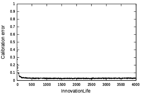
Figure 3. Profile of the parameter InnovationLife. - 4.2
- Under the value 150 the calibration error is higher than our validity threshold and then we consider that the model cannot be calibrated. From a thematical point of view: The deprecation of the innovations is too fast, thus the innovations cannot percolate in the system leading to unrealistic dynamics.
- 4.3
- Over the value 150 the obsolescence of the innovations is
slow enough to have no noticeable effect on the calibration of the
model. In particular when InnovationLife is set to
4000, the calibration error is lower than our acceptance threshold. For
this particular value, the matching mechanism of innovation
obsolescence could be considered as disabled: The maximum duration of a
simulation is 4000 steps, thus when InnovationLife
is set to 4000, the innovations are never considered deprecated. This
profile shows that this mechanism does not constrain much the model and
is useless to reproduce the expected dynamics. Seeking for a more
parsimonious model we have removed this mechanism. The following of the
article is based on the SimpopLocal model without the deprecation
mechanism.
Rmax
- 4.4
- The parameter Rmax
constraints the maximum size of settlements by limiting the impact of
the acquisition of an innovation on the size of a settlement. The
calibration profile for this parameter is shown on Figure 4.
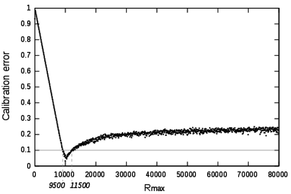
Figure 4. Calibration profile of the parameter Rmax. - 4.5
- The calibration objective for the size of the biggest settlement has been set to 10,000 inhabitants. When Rmax is set to a value lower than 10,000 it is impossible for the model to reach the 10,000 population objective. Thus, by construction, low values of this parameter can not achieve acceptable calibration errors.
- 4.6
- The profile exposes a narrowed range of very low calibration error between [9500;11500]. Surprisingly the calibration algorithm is not able to find low calibration errors for Rmax above 10,500. It indicates that this mechanism is necessary to produce acceptable dynamics and reaching settlements of a size matching empirical evidences.
InnovationImpact
- 5.1
- The InovationImpact parameter controls
the impact of the acquisition of an innovation on the growth of a
settlement. Figure 5
show
the calibration profile for this parameter. The section of the profile
containing low calibration errors is very narrowed, only 2 solutions
with calibration errors under 0.1 have been found. This profile has
been computed using the definition domain provided by the modellers
[0;2]. From Figure 5
it can
be deduced that the definition domain is too wide compared to the
validity domain for this parameter. Therefore another profile has been
computed for a much more restraint definition domain: [0;2.10-2].
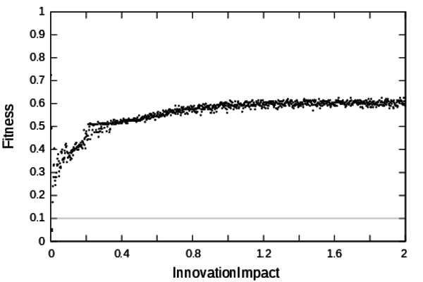
Figure 5. Calibration profile of the parameter InnovationImpact - 5.2
- The zoomed profile is shown on Figure 6.
It shows that when the impact on the settlement growth of the
innovation is too low the dynamic is too slow to reach the calibration
objectives. On the contrary, when InnovationImpact
is too high the growth of the settlements is too fast to match credible
dynamics (whatever the value of the other parameters can be). This
profile shows that the validity domain of this parameter is
[0.006;0.01].
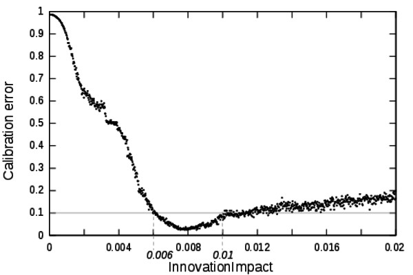
Figure 6. Detailed calibration profile of the parameter InnovationImpact
Pcreation
- 6.1
- The Pcreation
parameter determines the capacity of a settlement to create a new
innovations. Figure 7
shows
the calibration profile for this parameter. Once again the definition
domain given by the modellers [0;0.01] is too wide to establish
directly a validity domain. However, this profile shows that for high
values of Pcreation the
model can not reach low calibration errors. The inflexion of the
profile near the value 0 indicates that low calibration errors are
located in a much more narrowed domain close to 0.
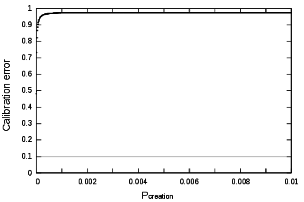
Figure 7. Calibration profile of the parameter Pcreation - 6.2
- Figure 8 shows
the calibration profile of the Pcreation
parameter within the domain [0;1e-5].
From this profile it can be deduced that the validity domain of Pcreation
is [0.4×10⁻⁶;2×10⁻⁶]. For
low values of Pcreation the
model can not be calibrated. The innovations are generated too slowly
to engender a sufficient growth (whatever the value of the other
parameters can be). For high values of Pcreation
the system races and growth is too fast.
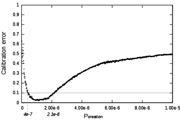
Figure 8. Detailed calibration profile of the parameter Pcreation
Pdiffusion
- 7.1
- The parameter Pdiffusion
governs the exchange of innovation between settlements. Figure
9 shows the calibration
profile for
this parameter which is very flat and contains only high calibration
errors. This profile exposes a shortcoming of the algorithm. If the
definition domain is very wide compared to the validity domain, the
method might take a lot of computation time to find the parameters
settings matching low calibration errors and give the false impression
that they don't exist. In the case of SimpopLocal we know that low
calibration errors exists because they were found when computing the
other profiles. By deduction from the model mechanisms, low calibration
errors should be found in a domain closer to 0.
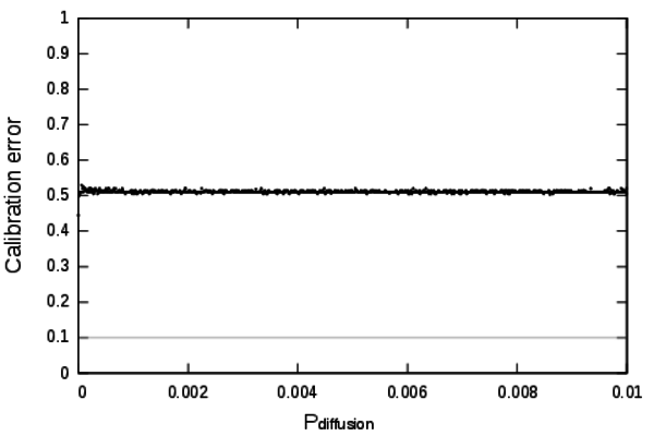
Figure 9. Calibration profile of the parameter Pdiffusion - 7.2
- The zoomed profile using the definition domain [0;10-5]
is shown on Figure 10. At this
scale the validity domain is revealed: [0.3
 10-6;1.810-6].
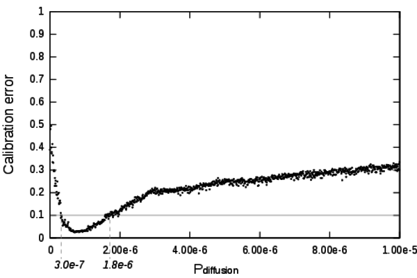
Figure 10. Detailed calibration profile of the parameter Pdiffusion - 7.3
- A very interesting aspect of this profile is that low values of Pdiffusion prevent the model from producing acceptable dynamics. Noticeably when Pdiffusion = 0 it disables entirely the diffusion mechanism of the model. At this particular point the calibration error is unsatisfying, thus this profile shows that the diffusion mechanism is mandatory in order to produce realistic behaviours.
DistanceDecay
- 8.1
- The parameter DistanceDecay acts on the
mechanism of diffusion of the innovations. It introduces a decaying
effect of the distance between settlements on the probability to
diffuse an innovation from one settlement to another. Figure 11 shows the calibration profile for
this parameter. High values of this parameter prevent the diffusion.
The calibration errors computed with high values of DistanceDecay
are almost equal to the calibration errors computed with Pdiffusion
set to 0 (that also inhibits the diffusion process). This matching
calibration error values provide an additonnal hint that the model and
its implementation are coherent.
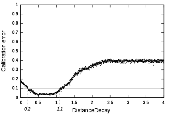
Figure 11. Calibration profile of the parameter DistanceDecay - 8.2
- The validity domain of DistanceDecay is [0.2, 1.1]. The mechanism piloted by DistanceDecay introduces a distance effect in the interaction process creating spatial heterogeneity. For low values of DistanceDecay the profile shows only unsatisfying calibration errors. It means that spatial heterogeneity is mandatory to produce acceptable dynamics.
Conclusion
- 9.1
- This paper proposes a new method to explore models. This
method, called Calibration Profile, computes 2-dimensional graphs that
depict the effect of each parameter on the model dynamics using a
calibration objective. It thus provides a global view of the local
effect of each parameter on the expected behaviour. This constitutes a
new form of sensitivity analysis of parameters on a calibration
objective that differs from classical sensitivity analysis methods (Saltelli et al. 2000).
Classical sensitivity analysis methods are based on statistical
analysis that are either local or global. Local sensitivity analysis
provides a measurement of the effect of the model parameters on the
outputs in a narrowed portion of the parameter space. Global
sensitivity analysis provides few aggregated global indicators of the
effect of each parameters in the whole parameter space. The CP method
produces a global picture of the local effect of a parameter on the
calibration objective all along its definition domain. Furthermore the
CP method seeks for extreme behaviours (the best ones) of the model and
that's why it is based on an optimisation algorithm. This kind of
information is not captured by classical sampling-based sensitivity
analysis. This CP method has been shown very useful to better
understand the dynamical behaviours of a geographical multi-agent
simulation model. It has lead to important novel understandings:
- The mechanism linked to the parameter InnovationLife of the model has been shown useless. This mechanism has thus been removed from the model, making it more parsimonious.
- Except from this mechanism all the other mechanisms (i.e spatial heterogeneity, diffusion of the innovations, creation of the innovations...) have been shown mandatory to produce acceptable dynamics. From a geographical point of view, these results are extremely interesting. They show how the consideration of space and of spatial interaction plays a central role in the simulation of credible settlement system growth dynamics.
- For all the parameters (InnovationLife excepted) a connected validity domain has been proposed, these boundaries are summarised in Table 2. The seemingly very narrow validity domain of several of those parameters (in particular InnovationImpact, pCreation, pDiffusion) is not preoccupying to our senses. On the one hand, this difference between the exploration domain and the validity domain can be directly assigned to the lack of empirical knowledge on the processes of innovation. Indeed the probability of innovation or even the impact of innovation adoption are not easily measurable variables in the real world, especially for the ancient periods that the model focuses on. Unsurprisingly the exploration domains that we defined a priori for these parameters has been found much larger than the actual validity domain. In the framework of the model hypothesis, it seems correct that these values are very small. Hence that seemingly very narrow validity domain of several parameters is not due to a lack of robustness of the model but rather to lack of knowledge and empirical measures that prevent the definition of a relevant observational scale. On the other hand, the value of those parameters is also directly linked to the definition of the concept of innovation implemented in the geographical model and to how we can quantify it (such as the average number of innovation per time period for example). Therefore the impact of each innovation is strongly related to the number of all considered/simulated innovations.
- 9.2
- This model exploration using the CP method has shown very
instructive on the model behaviour. More methodological development is
being achieved to include this method in an extensive modelling
framework encompassing several complementary tools for model
evaluations. We think that CP can play a significant role in modelling
methodologies such as KISS (Keep It Simple Stupid) for which the
simplicity of the models prevails. Using CP during the modelling
process may constitute a very efficient tool to achieve progressive
complexification of a very simple model towards a realistic one.
Table 2: Validity boundaries for SimpopLocal parameters Parameter Definition Validity domain Rmax [1;40, 000] [9, 500;11, 500] InnovationImpact [0;2] [6×10⁻³, 1×10⁻²] Pcreation [0;0.1] [4×10⁻⁷;2×10⁻⁶] Pdiffusion [0;0.1] [3×10⁻⁷;8×10⁻⁶] DistanceDecay [0;4] [0.2;1.1]
Acknowledgements
- This work is funded by the ERC Advanced Grant Geodivercity and the Institut des Systèmes Complexes Paris Île-de-France. The results obtained in this paper were computed on the biomed and the vo.complex-system.eu virtual organization of the European Grid Infrastructure (http://www.egi.eu). We thank the European Grid Infrastructure and its supporting National Grid Initiatives (France-Grilles in particular) for providing the technical support and infrastructure. We also thank the Réseau National des Systèmes Complexes (RNSC) and anonymous reviewers for their help in improving the first version of the paper.
Notes
-
1Let y
be the data and θ a vector of parameters that can
be decomposed as θ = (δ, ξ).
The likelihood function can be written as
 (θ| y)
= (δ,
ξ| y). If δ
is the parameter of interest, then the profile likelihood is the
function defined as Lp(δ)
=
(θ| y)
= (δ,
ξ| y). If δ
is the parameter of interest, then the profile likelihood is the
function defined as Lp(δ)
=  (ξ,
δ| y). See Pawitan (2001, p. 64) for a detailed
description.
(ξ,
δ| y). See Pawitan (2001, p. 64) for a detailed
description.
2https://github.com/ISCPIF/mgo
3http://scala-lang.org/
4www.openmole.org
5https://github.com/ISCPIF/profiles-simpoplocal
References
-
BEAUMONT, M. A. (2010). Approximate bayesian computation in evolution and ecology. Annual Review of Ecology, Evolution, and Systematics 41(1), 379–406. <>. [doi:10.1146/annurev-ecolsys-102209-144621]
BERRY, B. (1964). Cities as systems within systems of cities. Papers in Regional Science 13(1), 147–163. [doi:10.1111/j.1435-5597.1964.tb01283.x]
BRETAGNOLLE, A., Daudet, E. & Pumain, D. (2006). From theory to modelling : urban systems as complex systems. Cybergeo (335), 1–17.
BRETAGNOLLE, A. & Pumain, D. (2010). Simulating urban networks through multiscalar space-time dynamics: Europe and the united states, 17th-20th centuries. Urban Studies 47(13), 2819–2839. [doi:10.1177/0042098010377366]
BURA, S., Guerin-Pace, F., Mathian, H., Pumain, D. & Sanders, L. (1996). Multiagent systems and the dynamics of a settlement system. Geographical Analysis 28(2), 161-178. [doi:10.1111/j.1538-4632.1996.tb00927.x]
CLUNE, J., Mouret, J.-B. & Lipson, H. (2013). The evolutionary origins of modularity. Proceedings of the Royal Society b: Biological sciences 280(1755), 20122863. [doi:10.1098/rspb.2012.2863]
DEB, K. & Agrawal, R. B. (1994). Simulated binary crossover for continuous search space. Complex Systems 9, 1–34.
DEB, K., Agrawal, S., Pratap, A. & Meyarivan, T. (2002). A fast elitist non-dominated sorting genetic algorithm for multi-objective optimization: Nsga-II. IEEE Transactions on Evolutionary Computation 6.2, 182–197. [doi:10.1109/4235.996017]
DIAMOND, J. (1997). Guns, Germs, and Steel: The Fates of Human Societies. W. W. Norton & Company.
DURAND-DASTÈS, F., Favory, F., Fiches, J.-L., Mathian, H., Pumain, D., Raynaud, C., Sanders, L. & Van Der Leeuw, S. (1998). Archaeomedes: Des oppida aux métropoles. Paris: Anthropos.
FAVARO, J.-M. & Pumain, D. (2011). Gibrat revisited: An urban growth model incorporating spatial interaction and innovation cycles. Geographical Analysis 43(3), 261–286. [doi:10.1111/j.1538-4632.2011.00819.x]
FLETCHER, R. (1986). Settlement archaeology: World-wide comparisons. World Archaeology 18(1), 59–83. [doi:10.1080/00438243.1986.9979989]
GIBRAT, R. (1931). Les inégalités économiques. Librairie du Recueil Sirey, Paris.
GOLDBERG, D. E., Deb, K. & Rey Horn, J. (1992). Massive multimodality, deception, and genetic algorithms. Proceedings of Parallel Problem Solving from Nature 2 (PPSN 2), 37–46.
HINTERDING, R. (1995). Gaussian mutation and self-adaption for numeric genetic algorithms. In: Evolutionary Computation, 1995., IEEE International Conference on, vol. 1. IEEE. [doi:10.1109/icec.1995.489178]
LANE, D., Van Der Leeuw, S., Pumain, D. & West, G. (2009). Complexity Perspectives in Innovation and Social Change. No. 7 in Methodos Series. Springer, 1 ed. [doi:10.1007/978-1-4020-9663-1]
LENORMAND, M., Jabot, F. & Deffuant, G. (2012). Adaptive approximate Bayesian computation for complex models. <http://arxiv.org/abs/1111.1308>.
LIU, L. (1996). Settlement patterns, chiefdom variability, and the development of early states in north china. Journal of anthropological archaeology 15(3), 237–288. [doi:10.1006/jaar.1996.0010]
MAHFOUD, S. W. (1997). Niching methods. Handbook of Evolutionary Computation. [doi:10.1887/0750308958/b386c54]
MOURET, J. & Clune, J. (2012). An Algorithm to Create Phenotype-Fitness Maps. Proceedings of ALIFE pp. 593–595.
MOURET, J.-B. & Doncieux, S. (2012). Encouraging behavioral diversity in evolutionary robotics: An empirical study. Evolutionary computation 20(1), 91–133. [doi:10.1162/EVCO_a_00048]
PAWITAN, Y. (2001). In all likelihood: statistical modelling and inference using likelihood. Oxford University Press.
PUMAIN, D. (1997). Pour une théorie évolutive des villes. Espace géographique 26(2), 119–134. [doi:10.3406/spgeo.1997.1063]
PUMAIN, D. (2009). The evolution of city systems, between history and dynamics. International Journal of Environmental Creation 12(1).
PUMAIN, D. & Sanders, L. (2013). Theoretical principles in inter-urban simulation models: a comparison. Environment and Planning A 45, 2243–2260. [doi:10.1068/a45620]
REUILLON, R., Leclaire, M. & Rey, S. (2013). Openmole, a workflow engine specifically tailored for the distributed exploration of simulation models. Future Generation Computer Systems 29, 1981–1990. [doi:10.1016/j.future.2013.05.003]
ROBSON, B. (1973). Urban growth: An approach. London: Methuen ed.
SALTELLI, A., Chan, K., Scott, E. et al. (2000). Sensitivity analysis, vol. 134. New York: Wiley.
SANDERS, L., Pumain, D., Mathian, H., Guerin-Pace, F. & Bura, S. (1997). Simpop: a multiagent system for the study of urbanism. Environment and Planning B 24, 287–306. [doi:10.1068/b240287]
SCHMITT, C., Reuillon, R., Rey Coyrehourcq, S. & Pumain, D. (2014). Half a billion simulations: Evolutionary algorithms and distributed computing for calibrating the simpoplocal geographical model. Environnent and planning B: Planning and Design, advance online publication
SIMON, H. (1955). On a class of skew distribution functions. Biometrika 42(3/4), 425–440. [doi:10.1093/biomet/42.3-4.425]
STONEDAHL, F. J. (2011). Genetic Algorithms for the Exploration of Parameter Spaces in Agent-Based Models. Ph.D. thesis, Northwestern University of Illinois.
TOFFOLO, A. & Benini, E. (2003). Genetic diversity as an objective in multi-objective evolutionary algorithms. Evolutionary Computation 11(2), 151–167. [doi:10.1162/106365603766646816]
TURCHIN, P. (2003). Historical Dynamics: Why States Rise and Fall. Princeton University Press.
VERHULST, P. (1845). Recherches mathématiques sur la loi d'accroissement de la population. Nouveaux Mémoires de l'Academie Royale des Sciences et Belles-Lettres de Bruxelles (18), 1–41.
WILSON, A. (1971). A family of spatial interaction models, and associated developments. Environment and Planning 3(1), 1–32. [doi:10.1068/a030001]