Abstract

To increase profitability, farmers often decide to form strategic partnerships with other farmers, pooling their resources and outputs for greater efficiency and scale. These coordination decisions can have far-reaching and complex implications for overall food supply chain structural emergence, which in turn impacts system outcomes and long-term sustainability. In this paper, we describe an agent-based model that explores the impacts of farmer coordination decisions on the development of food supply chain structure over time. This model focuses on one type of coordination mechanism implementation method, in which coordinated farmer groups produce a single crop type and combine their yields to achieve economies of scale. The farmer agents' decisions to coordinate with one another depend on their evaluation of the tradeoff between their autonomy and the expected economic benefits of coordination. Each coordination decision is a bilateral process in which the terms of group reward sharing are negotiated. We capture the effects of farmers' size, income, and autonomy premia, as well as volume-price relationships and group profit-sharing rules, on the rate of farmer coordination and the number and size of groups that form. Results indicate that under many conditions, coordination groups tend to consolidate over time, which suggests implications for overall supply chain structural resilience.

Keywords:

Food Supply Chains, Sustainable Agriculture, Coordination, Agent-Based Modeling, Farmer Decision Making, Multi-Agent Simulation

Introduction

1.1

Individual farm-level decision making directly impacts large-scale food supply chain (FSC) outcomes and long-term sustainability, which are critical to human and environmental health. Because of the importance of these outcomes, many mathematical models have been developed to explore the impacts of farm management decisions on the FSC. These models typically study the relationship between farm inputs (e.g. crop selection, fertilizers, pesticides, water) and outputs (e.g. food yields, profits, pollutants), with an aim to inform policy and/or guide farmer decision-making. Many optimization models and, more recently, some agent-based models (ABMs) of farm management decisions have been developed for this purpose (see Ahumada and Villalobos (2009), Janssen and van Ittersum (2007), Weintraub and Romero (2006), and Krejci and Beamon (2012) for reviews).

1.2

While farm management decisions are indeed critical to FSC outcomes, farmer decisions regarding coordination with other FSC members – such as whether to coordinate, with whom, and how – are equally important. Although farm-level coordination decisions are motivated by individual farmers' objectives of increased profit and/or decreased risk (Gillespie & Eidman 1998; Key 2005), they can have far-reaching and complex implications for overall FSC structural emergence, which in turn impact the outcomes and long-term sustainability of the FSC. Of particular importance is the effect of farmer coordination decisions on the degree of FSC centralization. Highly-centralized FSC production and distribution can lead to efficiencies and economies of scale through large-scale production and distribution of food (Godfray et al. 2010); however, some argue that FSCs with decentralized and diverse structure are desirable because their lower resource intensity makes them inherently more stable and resilient (Dahlberg 2008). Coordination decisions also affect transportation decisions, which impact resource consumption (e.g., fuel). When farmers coordinate, they can consolidate their output and make more efficient transportation choices. However, large-scale coordination can encourage long-distance distribution of volumes that exceed regional demand, which can increase transport fuel consumption. Finally, these decisions impact social and economic measures amongst the farming community, in the forms of income and autonomy. Coordination can help farming communities build economic strength through scale, but if the implemented coordination mechanism involves significant losses to farmer autonomy, the net effect to the overall system can be negative (Renting et al. 2003; Lyson 2007). Because the types of coordination mechanisms that farmers choose to implement for individual benefit can have positive or negative impacts on overall FSC outcomes, understanding the factors that influence the choice of coordination mechanism is important.

1.3

Two types of coordination can occur among FSC members: 1) vertical coordination, which occurs among different FSC echelons, (e.g., between farmers and distributors) and 2) horizontal coordination, which occurs among members within the same FSC echelon. This paper focuses on farm-level horizontal coordination, in which farmers form strategic partnerships with other farmers to pool their resources and their outputs for greater efficiency and scale. Such coordination has become increasingly critical for small- and medium-sized farmers to remain profitable, enabling them to access markets in which customers prefer large and consistent volumes and to reduce costs through resource-sharing, particularly in post-harvest processing and distribution (Kirby et al. 2007). However, in deciding whether to coordinate, farmers must balance the potential benefits of coordination with the costs, which include the time, effort, and expenses involved with managing the coordination, as well as a loss of autonomy. This loss of autonomy is of particular importance, because autonomy is one of the most highly-valued aspects of the farming profession (Gasson 1973). In fact, farmers are often willing to sacrifice significant increases in income to maintain their autonomy (Gillespie & Eidman 1998; Key 2005).

1.4

Successful farmer coordination, in which all parties benefit from and are satisfied with the arrangement, depends on the selection and implementation of an appropriate FSC coordination mechanism. According to Xu and Beamon (2006), this depends on the coordinating farmers' operating environment, which is characterized by:

• Market factors, such as customer requirements, transport costs, and infrastructure
• Interdependence among the farmers, which can be characterized by the farmers' value of autonomy, their relative sizes, and their financial situations
• Environmental uncertainty, introduced through such factors as demand, prices, and weather
• Information technology in place/available, such as inventory management software to enable knowledge-sharing

1.5

The attributes of an appropriate coordination mechanism should match the characteristics of this operating environment. Per Xu and Beamon (2006), relevant coordination mechanism attributes include:

• The resource-sharing structure – possible values can range from no resource sharing among farmers, to operational-level information sharing, to a strategic alliance among coordinated farmers
• The decision style – possible values can range from centralized, in which one member has control and makes decisions for the coordinated group, to decentralized, in which each member makes decisions autonomously
• The level of control – possible values can range from a situation in which members follow strict rules and monitor each other frequently, to a situation in which there is very little monitoring
• Risk/reward sharing – possible values can range from a situation in which the risk-benefit ratio is fair, to a situation in which the risk-benefit ratio is unfair, with one member taking on less risk/responsibility but receiving more benefits

1.6

For successful coordination, farmers should select a coordination mechanism implementation method that best matches the desired coordination mechanism attributes. Depending on the operating environment and mechanism attributes, examples of implementation methods include:

• An informal coordination arrangement in which neighboring farmers share equipment and consolidate their products for efficient transport to market, with each farmer making autonomous decisions (including crop selection) and sharing revenues and costs fairly
• A formal coordination structure in which one farmer (the "grower-shipper") acts as a centralized consolidation, processing, and shipping point, creating contracts with supplier farmers to provide a designated crop type that is monitored by the grower-shipper for minimum quality/quantity standards, at a price that unfairly benefits the grower-shipper
• A cooperative coordination structure in which farmers coordinate to produce a variety of products to meet their customers' demands with profits shared fairly and equal votes among members

1.7

In all of these examples of farmer coordination mechanism implementation methods, being a part of the coordinated group provides benefits to its members, through shared and efficient use of resources, volume consolidation for better prices, and improved access to markets. However, in each of these examples, the coordinated farmers must pay some type of coordination management cost and lose some degree of autonomy as a result of coordination. Therefore, the decision to coordinate depends on how much a farmer's autonomy is worth to him, how much he stands to gain as a result of the coordination, and how much autonomy he will lose through the coordination, given the characteristics of the coordination partner(s) and the nature of the coordination mechanism.

1.8

In this paper, we describe an ABM that we use to study a specific farmer coordination mechanism and the degree to which it is implemented, given different operating environment characteristics. In particular, we study the effects of farmer size and autonomy preference, system pricing structures, and coordination rules on farmers' decisions to join and leave coordinated farmer groups. The results provide insight into the impact of individual-level farmer coordination decisions on overall FSC structure.

Methodology

2.1

To investigate the effects of farmer coordination decisions on the overall emergent FSC structure and outcomes, we have developed an ABM of a theoretical FSC (i.e., the network structure and input data values are entirely theoretical and are not based on an existing system) using NetLogo 5.0.2. ABM is well-suited to modeling farmer coordination in FSCs, allowing us to capture interactions among boundedly-rational farmers and the stochastic behavior of their environment. In this section, we describe the farmer agents and provide an overview of the full FSC model, followed by a detailed description of the sub-models that comprise the farmer coordination process and the experimental input parameters and values that were used to study this process. A summary of all model parameters is included in Table 1.

Table 1: Summary of model input parameters.
Parameter	Description	Possible Values	Uniform Values for all Farmer Agents?
ai	farmer i autonomy premium	experimentally varied	yes
gi	farmer i farm size (acres)	experimentally varied	experimentally varied
h	production cost ($/acre)	$10.00	yes
mi(min)	profit level at which farmer utility is minimum	$0	yes
mi(max)	profit level at which farmer utility is maximum	$40,000	yes
q	distributor pricing function coefficient	experimentally varied	yes
Qac	cost of changing from crop a to crop c ($)	$0 to $600	yes
ri	farmer i region number	0, 1, 2, or 3	no
Ri	farmer i risk tolerance	50,000	yes
trk	cost to transport from region r to region k ($)	$10.00 if r = k $100.00 if r ≠ k	yes
ui(min)	farmer i utility threshold	0.25	yes
vrc(med)	median crop c yield in region r (crop units/acre)	300, 400, or 500	no, varies regionally
vrc(min)	minimum crop c yield in region r (crop units/acre)	150, 200, or 250	no, varies regionally
vrc(max)	maximum crop c yield in region r (crop units/acre)	450, 550, 750	no, varies regionally
wc(med)	median crop c price ($/crop unit)	experimentally varied	yes
wc(min)	minimum crop c price ($/crop unit)	80% of median	yes
wc(max)	maximum crop c price ($/crop unit)	120% of median	yes
xi	farmer i x-coordinate	-1000 to 1000	no
yi	farmer i y-coordinate	-1000 to 1000	no
zrc(med)	median regional crop c demand (crop units)	250,000	yes
zrc(min)	minimum regional crop c demand (crop units)	225,000	yes
zrc(max)	maximum regional crop c demand (crop units)	275,000	yes
βdist	weight on coordination value distance component	0.9	yes
βprofit	weight on coordination value profit component	0.1	yes
π	weather factor mean value	1	no
σ	weather factor standard deviation	0.2	no

Farmer Agents

2.2

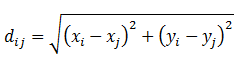
A single breed of agent participates in the coordination process: the farmer agent. 50 farmers in each of four distinct geographic regions (for a system total of 200 farmer agents) are assigned a farm size (g_i, in acres) and a unique set of x- and y-coordinates (x_i and y_i). These coordinates designate each farmer's position on a grid that ranges from −1000 to 1000 in both x and y directions, where one grid space is a single unit of distance. Each of the four geographic regions (r) is located in a different quadrant of this grid. To determine the distance d_ij between any two farmers i and j, the Euclidean distance is used:

(1)

2.3

Each farmer is assigned $10,000 at the start of each replication, and he begins the replication working independently (i.e., not as part of a coordinated group). The farmer's only objective is to select, grow, and sell crops to make as large a profit as possible to achieve the largest possible personal utility.

2.4

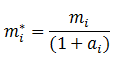
Each farmer is assigned an autonomy premium a_i (Gillespie & Eidman 1998; Key 2005), which represents how strongly the farmer values his ability to work independently. If farmer i is working independently, his current profit value (m_i^*) is simply the amount of profit (m_i) that he receives from selling his crops. However, if he is a member of a coordinated group, the value of his profit will be reduced by his autonomy premium (a_i):

(2)

2.5

For example, suppose that an independent farmer with an autonomy premium of 1 achieved a utility value of 0.80 as a result of acquiring $30,000 in profit last year. As a member of a coordinated group, that farmer would require $30,000 + ($30,000 * 1) = $60,000 dollars in profit in a given season to achieve a utility value of 0.80. Effectively, a farmer with an autonomy premium greater than zero will experience less utility from a given profit value when he is a group member than he would if he were working independently. In this model, it is assumed that farmers are predisposed to work independently (i.e., a farmer's autonomy premium is always positive).

2.6

Farmers each have a personal utility function, which maps profit values (m_i^*) to utility values (u_i). The form of the utility function is the same for all farmers in the system: an exponential utility function that is scaled such that u_i ranges from zero to one and increases monotonically over profit values m_i^* (Garvey 2008, pp. 71–74):

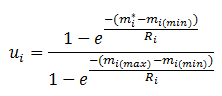
(3)

where m_i(min) and m_i(max) are the minimum and maximum profit parameter values for farmer i (i.e., the values at which the farmer experiences minimum and maximum utility, respectively), and R_i is the risk tolerance of farmer i. The value of R_i governs the shape of the utility function, such that u_i decreases with increasing values of R_i for a given profit value m_i^*. In this model, it is assumed that all farmers are risk-averse, and u_i is concave for all values of m_i^*. At the end of each time-step (i.e., growing season), the farmer's utility value is calculated and appended to his utility history list, which represents his "memory". Each season, this utility memory is accessed to determine the farmer's level of satisfaction, which will guide his strategic decision making regarding coordination – if the farmer's average utility over time falls below his threshold utility value (u_i(min)), he may decide to update his strategy.

Full FSC Model Overview

2.7

The farmer coordination decision process is one sub-model within a larger agent-based FSC model. Figure 1 shows all five main sub-models that comprise the overall model. At the beginning of a time-step (i.e., growing season), each farmer agent/group selects one of four different crop types to produce. The crop selection sub-model is run by each individual farmer agent in random order (since scheduling does not matter for the outcomes of the sub-model). In this process, each farmer estimates the value of each crop type, using a limited knowledge base. Unlike most crop selection models in the literature, in which farmers use optimization to make their decision, this sub-model presumes bounded farmer information and computational capacity. It is assumed that the farmer knows the overall system supply-demand ratio for each crop type, as well as median/expected values for prices, yields, and costs, and he uses this knowledge to make his crop value estimates and finally his crop selection decision.

2.8

The farmer's first step in the crop selection process is determining whether or not it is feasible to change from producing his current crop to another. If the farmer had no sales in the previous time-step (which can occur when system supply of a crop is greater than demand), he is allowed to consider changing crops. If his sales were greater than zero in the previous time-step, he is only allowed to change crops if he has been growing his current crop type for at least three consecutive time-steps. The farmer will next consider whether he has sufficient funds to change crop types, where the fixed cost of changing from the current crop a to crop c is Q_ac. The value of Q_ac depends upon the values of a and c and ranges from $0 (when a = c) to $600, representing the variability in the costs that are associated with switching from one crop to another (e.g., for acquiring new planting/harvesting equipment and/or training employees to use new production techniques). For example, switching between two similar crops (e.g., potatoes and carrots) would be less costly than switching to a dissimilar crop. If the farmer can afford Q_ac, he will add crop c to his set of feasible alternatives. After this analysis, if the feasible set only contains the farmer's current crop, the farmer will be forced to continue producing the same crop that he produced in the previous time-step.

2.9

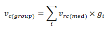
If the feasible set contains at least one alternative to the current crop, the farmer will calculate opportunity values (o_c) for the crops in the feasible set to help him decide which crop type to produce next season. Each opportunity value (o_c) is based on 1) the estimated profit for the coming season from growing crop c, given that the farmer/coordinated farmer group sells its entire expected yield and 2) the estimated market opportunity value for crop c for the coming season. To calculate the estimated profit for each feasible crop type, the farmer first estimates the potential yield (v_c(group), measured in "crop units"). If the farmer is a member of a coordinated group, he estimates v_c(group) for the entire group by multiplying the median yield per acre in the group's own region (v_rc(med)) by each member farmer i's farm size (g_i) and then summing these values:

(4)

2.10

If the farmer is working independently, the estimated yield value (v_c(group)) is simply an estimate of the farmer's own yield. The estimated profit (m_c(group)) for crop type c is the estimated yield (v_c(group)) multiplied by the median unit price for crop c (w_c(med)), minus the average cost of transporting crops (t_rk) from the farmer's/group's own region (r) to distributor k (where transport cost is assumed to be independent of crop type and volume):

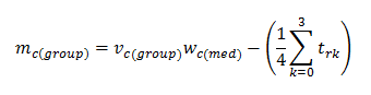
(5)

2.11

Once he has estimated the overall profit (m_c(group)), the farmer will then use this value to estimate his own individual profit from crop c (m_c(ind)). He first multiplies the overall profit (m_c(group)) by the percentage that represents his profit share (α, which is equal to 1 if the farmer is working independently). From this value, the farmer will then subtract his estimated individual cost, which is his production cost per acre (h) multiplied by his farm size (g_i), plus the cost of changing from the current crop a to crop c (Q_ac) annualized over three years. The resulting value is then multiplied by the farmer's crop inertia premium (λ) to calculate m_c(ind), his individual profit estimate for crop c:

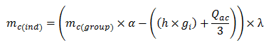
(6)

2.12

If the crop under consideration (crop c) is the farmer's current crop, then λ = 1; that is, the inertia premium has no effect on crop c's estimated profit value to the farmer. If crop c is different from the farmer's current crop, the value of the inertia premium depends on the number of consecutive years that the farmer has produced his current crop. The inertia premium is set to 1 in the first year of production, and each consecutive year that the farmer produces that crop thereafter, it is decremented by 0.1 (to a minimum value of 0.1). Therefore, the inertia premium devalues the estimated profit of crops other than the current crop.

2.13

The opportunity value for crop c (o_c) is calculated as a percentage of the farmer's estimated individual profit from crop c (m_c(ind)). The value of the percentage depends on the current ratio of system-wide supply (S_c) to system-wide demand (D_c) for crop c, such that the opportunity value and the supply-demand ratio are inversely proportional.

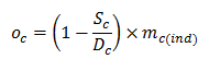
(7)

2.14

The farmer calculates the opportunity value (o_c) for all crop types in the feasible set of alternatives, and the crop type with the largest opportunity value is the farmer's preferred crop. If the farmer is not working as part of a coordinated farmer group, at this point he simply assigns himself his most preferred crop for production in the coming season. However, if he is a member of a group, he and the other farmers in his group will select the crop collectively through a vote. Each individual farmer will cast his vote, which is weighted by the farmer's differential value (δ_i(critical), the assignment of which is described in the next section of this paper). The crop type with the greatest number of votes is then assigned to all group members. If a farmer cannot afford to switch to the group's preferred crop type, he will leave the group and will continue to work independently, producing the crop that he grew in the previous time-step.

2.15

Each farmer i then produces his selected crop c, with a total yield (v_ci^*, measured in "crop units") that is based on farm size, weather, and regional effects. To determine v_ci^*, each farmer's base yield per acre (v_ci) is drawn from a triangular distribution that has regionally-specific parameters (v_rc(min), v_rc(med), v_rc(max)) to simulate the differences in regional suitability for each crop type (e.g., soil characteristics). This base yield per acre is then multiplied by the farmer's total farm size in acres (g_i) to obtain the farmer's overall base yield. A regional weather factor (ω_r) is then drawn from a truncated normal distribution (such that ω_r ≥ 0) with mean μ and standard deviation σ. This weather factor and the farmer's overall base yield are then multiplied to obtain the total yield:

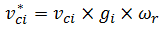
(8)

2.16

Wholesale unit prices (w_c) for each crop type c are then drawn from a triangular distribution that has parameter values (w_c(min), w_c(med), w_c(max)) that are uniform across all regions and crop types. Regional demand for each crop type (z_rc) is also drawn from a triangular distribution, with parameter values (z_rc(min), z_rc(med), z_rc(max)), which are also uniform across all regions and crop types. Although the unit prices and demand values are subject to randomness to simulate real-life system variability, their determination is exogenous to the model (i.e., it is assumed that there is no relationship between price and demand).

2.17

If a farmer is a member of a coordinated group, he will transport his crop yield to the group's leader for consolidation. Each farmer/group then sells as much of its yield as possible to regional distributor agents through a process of negotiation. It is assumed that a farmer/group will always choose to fulfill demand for its crop in its own region first (based on the assumption that transport costs are less); if there is remaining inventory after this sale, the farmer/group will sell to other regions. Through this process, each farmer acquires sales revenue, and the difference between his revenue and his production costs is his annual profit (m_i). After all the farmer agents/groups have sold their crops, each farmer evaluates his profits and corresponding utility values. A farmer's profit drives his decisions on crop choice for next season, and his utility value influences his decision to coordination with other farmers. After making these decisions, the process begins again with the start of a new time-step (i.e., growing season). In the next section, we will describe the farmer coordination process in more detail.

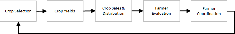
Figure 1. Flowchart representation of the overall FSC model (single time-step).

Farmer Coordination Process

2.18

Because the objective of each farmer agent is to acquire as much annual profit as possible, and farmers prefer to work independently, it follows that for farmers to decide to coordinate with one another, there must be an incentive for doing so that has the potential to increase a farmer's annual profit. As a representation of the size and volume advantages that exist in real life (i.e., higher volumes typically result in better prices and better access to markets), a volume-based pricing function is used to determine the unit price that farmer i will be paid (w_ci) for selling volume v_ci. Specifically, w_ci increases as the percentage of the regional distributor's overall demand for crop c (z_rc) that can be filled by farmer i's yield of crop c (v_ci) increases. The rate at which w_ci increases with increasing volume depends on q, which represents the strength of distributor preference for large volumes. It is assumed that the value of q is the same for all distributors across all regions. When q is large, the relationship between volume and price is strong (i.e., the unit price that a distributor is willing to pay becomes directly proportional to the volume as q→∞). It is assumed that w_ci is an exponential function of q, z_rc and v_ci, with a lower bound of zero (when v_ci = 0) and an upper bound equal to the wholesale unit price for crop c (w_c) when v_ci = z_rc:

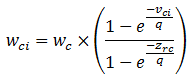
(9)

2.19

This pricing function is known to all farmers. The relationship between unit price and volume gives farmers an incentive to coordinate with other farmers – coordinated groups consolidate their crops before selling, giving them a volume and price advantage over independent farmers. It is assumed that a farmer can only be a member of one coordination group at a time, contributing his entire yield to that group, and that the group only produces one crop type at a time.

2.20

Figure 2 shows the farmer coordination process, which begins with each farmer agent assessing his group status (i.e., independent or a member of a coordinated group) and his utility. If the farmer is currently working independently, and if after three seasons of independent production he has found himself to be "dissatisfied" on average (i.e., his utility is below his threshold value u_i(min)), he will begin to seek out other farmers for coordination. Farmer i begins this process by ranking the other farmers/groups in his region. To accomplish this, he assigns each farmer/group j in his region a coordination value (θ_j), where larger values of θ_j result in a higher ranking. The coordination value is a function of two components: farmer/group j's profit and its geographic distance from farmer i. θ_j increases with increasing profit, indicating a farmer's preference to coordinate with financially successful farmers/groups. Geographic proximity also increases a potential coordination partner's value, which mirrors real-life farmers' preferences to work with others that they know and that are located in their own community (Gillespie & Eidman 1998). In this way, the distance between farmers is a proxy for trustworthiness.

2.21

To determine the profit component of the coordination value for each farmer/group j in his region (θ_j(profit)), farmer i assesses the current profit of each agent (m_j) and records the largest of these profit values (m_j(max)). It is assumed that farmer i has perfect knowledge of these values. Farmer i then calculates the ratio of m_j to m_j(max) for each farmer/group j (to assess its relative profitability), and this ratio is multiplied by a profit component weight (β_profit) to determine the profit component:

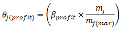
(10)

2.22

To determine the distance component (θ_j(distance)), farmer i first calculates the Euclidean distances between himself and all other farmers/groups in his region (d_ij) and records the largest of these distances (d_ij(max)). Then, the ratio of d_ij to d_ij(max) is calculated and subtracted from 1 (because smaller values are preferred, but the ranking is based on "the-larger-the-better" values of the distance component), and this difference is multiplied by the distance component weight (β_dist), where β_dist + β_profit = 1:

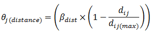
(11)

2.23

The coordination value θ_j is the sum of the distance value component and the profit component:

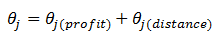
(12)

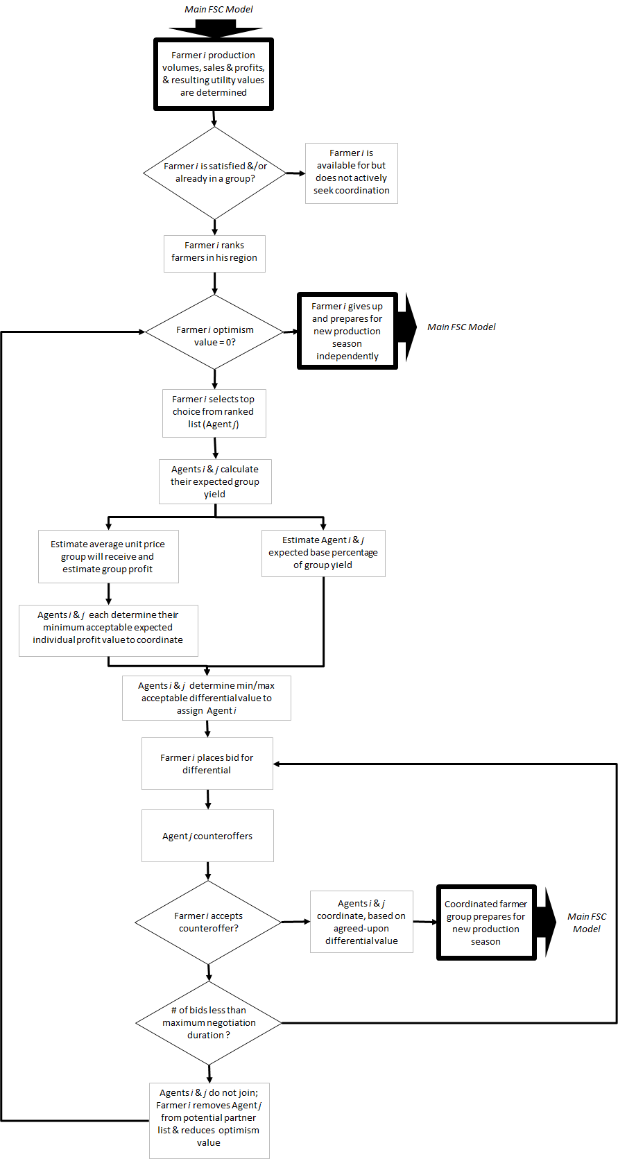
Figure 2. Flowchart representation of the farmer coordination process.

2.24

In this model, β_dist = 0.9 and β_profit = 0.1 for all farmer agents; that is, geographic proximity is weighted much more heavily than profitability. The set of potential collaborating farmers is then ranked in descending order by θ_j (i.e., larger values of θ_j are more preferred).

2.25

Farmer i selects the most highly-ranked farmer/group in his region (farmer/group j^*), which cannot have been rejected by farmer i in any previous searches in the current season. Next, agents i and j^* calculate their expected combined yield (v_group). If agents i and j^* produced the same crop c in the previous season, this value is estimated based on both agents' actual yields (which are assumed to be known to both parties). If agents i and j^* produced different types of crops in the previous season, their expected combined yield (v_group) is determined using farmer i's actual yield of crop c last season and the expected yield of crop c for agent j^*. The expected yield of agent j^* is estimated using Equation 4 (i.e., by multiplying the median yield per acre for crop c by the farm size of each farmer member of agent j^*, and then summing these values). The expected combined yield (v_group) is then applied to the pricing function given in Equation 9 to determine the expected unit price the group would receive collectively from the distributor (w_group). The expected group yield and unit price are then multiplied to determine the group's expected profit (m_group). For farmer i to be willing to coordinate with farmer/group j^*, this value must be at least as large as farmer i's current profit plus an added premium that accounts for his loss of autonomy. Farmer i calculates this minimum acceptable expected individual profit (m_i(critical)) that would convince him to coordinate with farmer/group j^* by rearranging Equation 2 and applying his own current profit (m_i) and autonomy premium (a_i):

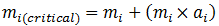
(13)

2.26

If agent j^* is an independent farmer, he will similarly calculate his own minimum acceptable expected individual profit (m_j(critical)). If agent j^* is a coordinated group, it is assumed that the group has no autonomy premium and is guaranteed to benefit from gaining farmer i as a new member. For agents i and j^*, if their expected share of the expected group profit does not exceed their minimum acceptable expected individual profit, the only way that they will consider coordinating is to negotiate a profit premium that will give them an extra share of the group profits. For farmer i, this extra share is δ_i(critical), the "differential":

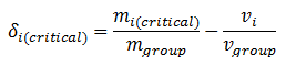
(14)

where v_i and v_group are the expected farmer i and potential group yields, respectively. A non-zero differential indicates unfair sharing of profits; δ_i(critical) will be positive if the farmer's current profit is larger than expected, negative if the current profit was less than expected, and zero if the current profit equals the expected profit. This suggests that if a farmer is doing poorly, he will be willing to give up some of his fair share just to enable him to join the group. The concept of using a differential as a basis for negotiation is based on the work of Reynolds (1997) and Staatz (1986), which describe the possibility for farmer groups to entice new members with a differential premium if it is worthwhile for the group to give up some of their fair share of profits to gain the benefit of the new member's volume.

2.27

At this point, agents i and j^* begin negotiating the value of the differential δ_i that farmer i will be assigned upon coordination. Farmer i begins the negotiation process by bidding the maximum differential that he can reasonably expect, which is the value of farmer/group j^*'s entire expected share of profits. Agent j^* counteroffers by bidding the minimum differential that it would be willing to give up to farmer i. If farmer i rejects agent j^*'s counteroffer, he will respond with a bid that is the midpoint between 1) his most recent bid and 2) either farmer/group j^*'s most recent bid or farmer i's critical value (δ_i(critical)), whichever is larger.

2.28

Farmer/group j^* will respond in kind, and this process will continue until either 1) the difference between their bids is less than a predetermined amount, in which case they reach agreement, or 2) a predetermined maximum duration of bidding has been reached, in which case agents i and j^* are unable to agree on an acceptable differential. If the negotiation is successful, this indicates that agents i and j^* believe that coordinating at the agreed-upon differential value is expected to benefit them, and farmer i joins farmer/group j^* in a new coordination group. In this case, farmer i has a three-year "contract" with farmer/group j^* – if farmer i is dissatisfied on average during this three-year period, he can choose to leave the group and begin producing independently again.

2.29

If the negotiation is unsuccessful, farmer i's "optimism" level is reduced. Farmer i then selects the next best choice from his ranked list and begins the search process again, continuing this iteratively until he either successfully coordinates with another farmer/group or his optimism level is reduced to zero, whereupon he gives up and decides to continue producing independently next season.

Experimental Inputs

2.30

Given the importance of farm-level coordination decisions, understanding the degree to which farmers select coordination over remaining independent and the resulting impact of these decisions on FSC structure are of interest. The model was used to run experiments to test the impact of different farmer size distributions, autonomy premium values, crop prices, price-volume function structure, and coordination rules on these outputs. Experiments were performed for all possible combinations of input parameter levels, for a total of 72 experiments. Each experiment was run for 30 replications of 300 discrete time-steps, where each time-step represented a "growing season" in which the entire cycle of crop production and distribution (i.e., planting, harvest, sale, and transport) and farmer decision making (i.e., coordination strategy and crop selection) occurred (as shown in Figure 1). A value of 300 time-steps was chosen for the replication length to allow sufficient time for the system to reach a steady state. The details of these five input parameters are provided below:

• Farm size distribution (f): This input parameter has two levels: when its value is set to zero, farm sizes are variable (with five 100-acre farms, 15 50-acre farms, and 30 25-acre farms in each region), and when its value is set to one, farm sizes are uniform (with 50 25-acre farms in each region).
• Median selling price per crop unit (w): In each time-step, the unit price for each crop is drawn from a triangular distribution, with a median value that has three possible experimental levels: low ($0.10), medium ($1.00), or high ($5.00).
• Farmer autonomy premium (a): The farmer autonomy premium has three levels: low (0.25), medium (2) and high (4). For any given experimental setting, all farmers in the system are assigned the same autonomy premium value, and this value does not vary over the course of a replication. Lower values represent increased farmer willingness to coordinate, while higher values represent increased farmer desire for independence.
• Distributor pricing function coefficient (q): The pricing coefficient can be either low (1,000) or high (50,000). When it is low, the regional distributor places a lower value on volume, and there is not much difference between the prices offered to a seller with low volume and a seller with high volume. In contrast, when the pricing coefficient value is high, a seller with a large volume will receive a large price advantage over a seller offering a low volume.
• Coordinated farmer share calculation (s): This parameter has two experimental levels: zero or one. When it is set to zero, farmers who are considering coordination will plan to share their group profits fairly (e.g., if one group member produces 60% of the group's volume, then that farmer will receive 60% of the group's profits). In this case, the farmers will skip the process of negotiating the differential value, and the coordination decision will be based on each party's comparison of his expected fair share of the expected group profit to his minimum expected profit – if both parties are satisfied, they will form a group. In contrast, when this parameter is set to one, coordinating farmers will follow the negotiation process previously described to determine each member's profit share.

2.31

Table 2 provides a summary of the experimental values of the input parameters.

Table 2: Experimental input parameters and values.
Factor	Description	# of Levels	Experimental Values
f	farm size distribution	2	variable, uniform
w	median selling price per crop unit	3	$0.10, $1.00, $5.00
a	farmer autonomy premium	3	0.25, 2, 4
q	distributor pricing function coefficient	2	1000, 50000
s	coordinated farmer share calculation	2	fair, negotiated

Results

3.1

For each experiment, three output metrics were captured to provide information about the overall structure of the FSC in a given time-step:

• Percent grouped farmers (pg): This metric captures the percentage of all farmers in the system who are members of a coordinated group (i.e., not working independently) at the end of each time-step.
• Total number of farmer groups (ng): At the end of each time-step, the total number of coordinated groups in the system having more than one farmer member are counted.
• 90^th percentile farmer group size (gs): This metric captures the size (i.e., number of members) of the farmer group at the 90^th percentile in each time-step. This value provides some indication of the distribution of farmer group sizes.

3.2

Each reported output metric value is an average value over the 30 replications. Two different types of results are presented here: 1) final output values that were captured in the 300^th time-step, and 2) output values captured in each time-step over the entire 300-step replication. The final output values for each experiment were analyzed statistically (using ANOVA and evaluating statistical significance at a at a 95% confidence level), and plots of mean output values over the entire replication length were generated and analyzed graphically. These plots can be found in the Appendix.

Percentage of grouped farmers

3.3

Figure 3 shows the main effects of each of the five experimental input parameters on the percentage of farmers that were members of coordinated groups (pg) after 300 time-steps, and Table 3 provides the ANOVA output. As Table 3 shows, all five input parameters had statistically significant impacts on pg (p-value = 0.0 for f, w, a, q, and s), and these parameters accounted for a large proportion of the total variability that was observed in pg (R² = 71.5%). The farm size distribution parameter (f) had the largest impact on pg (F-value = 1716.3), with a statistically-significant difference between the experiments in which the farmers in each region varied in size (f = 0) and the experiments in which the farmers were uniformly small in size (f = 1). When the farmers were of variable sizes, at the end of 300 time-steps, on average 61.1% of the farmers in the system were members of coordinated groups. In contrast, when the farmers were all small-sized, 24.3% of the farmers were grouped. The unit price (w) and the pricing coefficient (q) also impacted farmer grouping behavior (F-value = 991.2 and 901.1, respectively). Increases in w led to increased values of pg: 21.8% of farmers were in groups when the price was lowest (w = $0.10), 37.0% when the price was medium (w = $1.00), and 69.2% when the price was highest (w = $5.00). Unsurprisingly, pg also increased with increasing values of pricing coefficient (q), with 29.3% of farmers grouped when q was low (q = 1,000) and 56.0% grouped when q was high (q = 50,000). Farmer autonomy premium values (a) also affected farmer grouping, although not nearly as much as the farmer size distribution or price (F-value = 391.9). As expected, pg decreased significantly (and linearly) with increasing autonomy premium values, with 58.7% of farmers in groups when the autonomy premium was low (a = 0.25), 40.8% when it was at a medium level (a = 2), and 28.5% when it was highest (a = 4). Although s, the method of calculating coordinated farmer share (i.e., fair or negotiated), had a statistically-significant effect on pg, its impact was relatively small (F-value = 15.1).

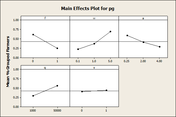
Figure 3. Main effects plot for percent grouped farmers (pg).

Table 3: ANOVA output for percent grouped farmers (pg).
Source	DF	SS	MS	F-value	p-value	R-Sq
f	1	73.0	73.0	1716.3	0.0
m	2	84.4	42.2	991.2	0.0
a	2	33.4	16.7	391.9	0.0
q	1	38.3	38.4	901.1	0.0
s	1	0.6	0.6	15.1	0.0
Error	2152	91.6	0.0
Total	2159	321.3				71.5%

Total number of farmer groups

3.4

Figure 4 shows the main effects of the experimental parameter values on the mean number of farmer groups in the system after 300 time-steps (ng), and Table 4 shows the corresponding ANOVA output. As with pg, all five input parameters had statistically-significant impacts on ng (p-value = 0.0 for f, w, a, q, and s). However, the model did not account for much of the total variability that was observed in ng (R² = 32.7%), and the source of nearly all of this variation was f, the farmer size distribution parameter (F-value = 788.0). As with pg, ng was significantly larger when the farmer size distribution was variable (10.4 groups), compared with the experiments in which all farmers were small-sized (3.4 groups). The autonomy premium (a) had a smaller effect (F-value = 92.1), with the mean number of groups decreasing as the value of a increased (9.2, 6.1, and 5.3 groups for low, medium, and high values of a, respectively). The method of calculating coordinated farmer share (s) also had a small but significant effect (F-value = 52.7), with fewer groups (6.0 groups) forming when profits were shared fairly than when the profit share was negotiated (7.8 groups). The impacts of selling price (w) and the price function coefficient (q) on ng were very small (F-value = 4.0 and 14.3, respectively).

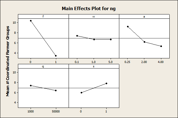
Figure 4. Main effects plot for number of coordinated farmer groups in the system (ng).

Table 4: ANOVA output for number of coordinated farmer groups in the system (ng).
Source	DF	SS	MS	F-value	p-value	R-Sq
f	1	26446.0	26446.0	788.0	0.0
m	2	265.0	132.5	4.0	0.0
a	2	6184.2	3092.1	92.1	0.0
q	1	479.8	479.8	14.3	0.0
s	1	1767.6	1767.6	52.7	0.0
Error	2152	72227.5	33.6
Total	2159	107370.1				32.7%

90^th percentile farmer group size

3.5

Figure 5 shows the main effects of the five experimental input values on the 90^th percentile farmer group size (gs) after 300 time-steps, over 30 replications, and Table 5 shows the corresponding ANOVA output. In this case, four of the five input parameters (f, w, a, and q) were statistically significant (p-values = 0.0), s was not (p-value = 0.6), and together they accounted for 51.6% of the variability observed in gs. In contrast with pg and ng, the input parameter with the greatest influence on gs was the price function coefficient, q (F-value = 1080.6). The mean 90^th percentile group size was much smaller when q was low (9.4 farmers/group) than when q was high (27.1 farmers/group). The farmer size distribution (f) also had a large impact on gs (F-value = 420.3), with larger groups forming when the farm size distribution was variable (23.8 farmers/group), compared with a distribution of uniformly small-sized farmers (12.8 farmers/group). Selling price (w) also had a strong impact on group size (F-value = 335.9), with a relatively value of gs at the lowest price level (9.8 farmers/group), a larger mean group size at the medium price level (18.1 farmers/group), and the largest group size at the highest price level (26.9 farmers/group). The autonomy premium value (a) had a much smaller effect (F-value = 58.7), with gs decreasing slightly with increasing values of a. At the low, medium and high levels of a, the gs was 21.6, 18.8, 14.5 farmers, respectively.

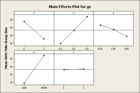
Figure 5. Main effects plot for the 90th percentile coordinated farmer group size (gs).

Table 5: ANOVA output for the 90th percentile coordinated farmer group size (gs).
Source	DF	SS	MS	F-value	p-value	R-Sq
f	1	65781	65781	420.3	0.0
m	2	105141	52570	335.9	0.0
a	2	18372	9186	58.7	0.0
q	1	169106	169106	1080.6	0.0
s	1	42	42	0.3	0.6
Error	2152	336780	156
Total	2159	695222				51.6%

Discussion

4.1

Farmer size distribution (f) heavily influenced farmer coordination decisions, with results indicating that a system with variable farm sizes encourages more farmer coordination and the formation of larger groups than a system composed of uniformly small-sized farms. The differences between variable and uniform farm size distribution are not very pronounced when the volume-price coefficient value is large (q = 50,000); in either case, farmers were sufficiently motivated to coordinate. However, when q was small (q = 1,000), the uniform system (f = 1) produced significantly fewer and smaller groups than the variable system (f = 0). That is, for the system with variable farm sizes, farmers' decisions to coordinate were relatively insensitive to q, whereas the system with all small farms showed substantial coordination for large q and very little coordination for small q. This outcome is likely partly a result of the pairwise nature of the farmer coordination process. For example, when a small farmer considers coordinating with a much larger farmer, the small farmer immediately perceives that their combined volume will result in a significant price advantage for him – even for small values of q. In contrast, when two small farmers consider coordinating, their combined volume will only result in a significant price advantage if q is large. Because two independent farmers can only estimate the immediate value of their forming a partnership (i.e., they cannot foresee the potential future advantage of forming a multi-farmer coordination group over time), when q is small and both farmers are small in size, the farmers are unlikely to coordinate, which precludes the formation of any multi-farmer groups. Future development of the model's coordination process will overcome this limitation by giving the farmer agents the foresight necessary to allow them to be more strategic in their coordination decisions, and/or allowing multiple farmers to negotiate coordination simultaneously.

4.2

While the unit selling price (w) had very little effect on the total number of farmer groups that formed, increases in unit price (and therefore farmer profitability) significantly increased the percentage of farmers that joined coordinated groups, as well as the size of those groups, after 300 time-steps. This result is most striking when the unit price is highest. As shown in Figure 6, when the unit price is $5.00 and the farmer size distribution is variable, nearly all farmers in the system are members of a coordinated group after the 100^th time-step, regardless of other input parameter levels. Figure 7 shows an example of the 90^th percentile farmer group sizes when the unit price is $5.00. Interestingly, this value increases with increasing autonomy premium value, with the majority of farmers consolidated into one very large regional group. Once these groups have formed, they appear to remain stable throughout the replication. These results indicate that when prices and profits are high and farmers are satisfied, although they might not immediately decide to coordinate, once they do coordinate, they remain satisfied and have no incentive to leave their group.

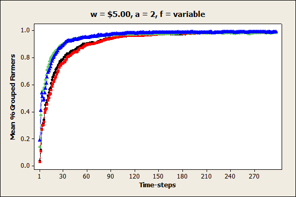
Figure 6. Mean percent grouped farmers (pg) in each time-step when price per unit is high, autonomy premium is medium, and farm size distribution is variable.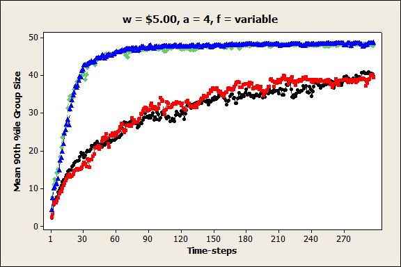

Figure 7. Mean 90th percentile farmer group size (gs) in each time-step when price per unit is high, autonomy premium is high, and farm size distribution is variable.

4.3

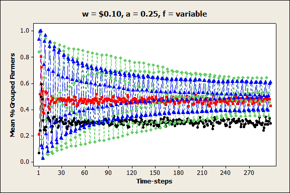
Unsurprisingly, increasing the values of the farmers' autonomy premia tended to result in reduced farmer coordination, with fewer and smaller groups forming. This result was most pronounced when prices were at low and medium levels (w = $0.10 and $1.00). A more interesting result was the effect of autonomy premium values on group volatility. For example, Figures 8a and b show that when the unit price was low (w = $0.10), the percentage of grouped farmers and the 90^th percentile group size were extremely variable from one time-step to the next when the autonomy premium was low (a = 0.25), but these values were fairly stable when the autonomy premium was high (a = 4). In contrast, Figures 9a, b, and c show that when the unit price was at a medium level (w = $1.00), the percentage of grouped farmers was stable when the autonomy premium was low or high, but it was highly variable when the autonomy premium was at a medium level. This increased variability only occurred when the pricing function coefficient was large (q = 50,000). These results suggest that under certain conditions, farmers are ambivalent about coordination – they are unable to reconcile their desire for autonomy with their need for profitability, and as a result, they repeatedly join and leave groups over time.

(a)                                                                                                (b)

Figure 8. Mean percent grouped farmers (pg) in each time-step when price per unit is low, farm size distribution is variable, and autonomy premium is a) low and b) high.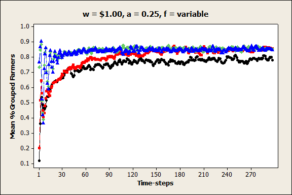

(a)                                                                                                (b)

(c)

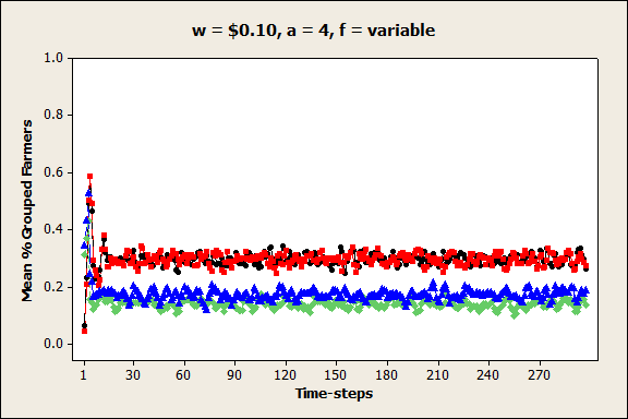
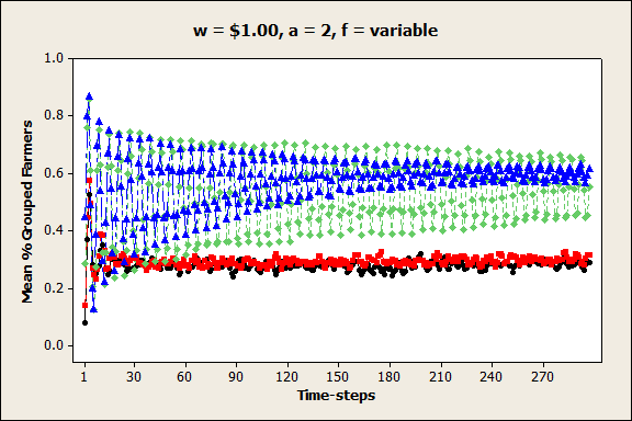
Figure 9. Mean percent grouped farmers (pg) in each time-step when price per unit is medium, farm size distribution is variable, and autonomy premium is a) low, b) medium, and c) high.

4.4

Predictably, farmer groups tended to be significantly larger when the volume-price relationship was strong (i.e., when q = 50,000). In most cases, the coordination rule (s) did not influence farmer coordination much. However, when the unit price, the autonomy premium, and the pricing function coefficient values were low (as seen in Figure 10), the number of farmer groups that formed was significantly larger when the profit-sharing terms were determined through negotiation (s = 1). For this particular experiment, it seems that negotiated terms benefited larger farmers sufficiently to make coordination worthwhile for them, and the smaller farmers were willing to accept a small share, because they were receiving low prices and were relatively unconcerned with maintaining their autonomy.

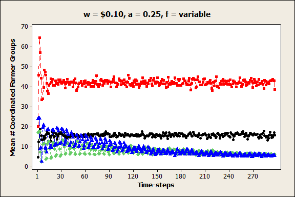
Figure 10. Mean number of coordinated farmer groups (ng) in each time-step when price per unit is low, farm size distribution is variable, and autonomy premium is low.

Conclusion

5.1

Farmer coordination decisions have a significant impact on FSC performance and structural emergence over time. In this paper we have described the farmer coordination decision process of an FSC ABM, and we have demonstrated its usefulness in studying the impacts of farm size distribution, farmer autonomy premia, prices, price-volume relationships, and group profit-sharing rules on farmers' decisions to coordinate with one another. The results of these experiments provide insight into the ways in which farmer coordination decisions impact FSC outcomes and structure, including the evolution of the percentage of farmers that decide to coordinate and the number and size of farmer groups that form over time. This paper focused on one type of coordination mechanism implementation method, in which coordinated farmer groups produce a single crop type and combine their yields to achieve economies of scale. This type of coordination can improve economic sustainability for individual farmers (especially small-sized farmers). However, in real-life food systems, the financial incentives that motivate farmers to pursue economies of scale have also encouraged the development of regional monocultures, thereby reducing regional crop diversity. Exploring the relationships among farmer coordination decisions, regional crop diversity, and overall food system resilience to external threats (e.g., natural disasters) is the subject of ongoing model development and experimentation.

5.2

Future work will also consider other coordination possibilities, in which crop variety is valued. This would allow for coordination mechanisms that could potentially benefit farmers and also support regional crop diversity. Studying the effects of high variability of demand, prices, and yields on farmer coordination and subsequent FSC outcomes is also of interest. Additionally, the impact of vertical coordination among farmers and other FSC echelons will be captured. Data-gathering from an existing food system (e.g., farmer surveys, network structural analysis) in central Iowa is the subject of ongoing work, with an aim to develop and validate the theoretical model described in this paper to become a useful analysis tool for a real-life system. Agent-based modeling allows us to gain a better understanding of the impact of individual-level coordination decisions on emergent FSC properties, which can be used in support of guiding individual decisions and policy toward a resilient and sustainable food supply.

Appendix

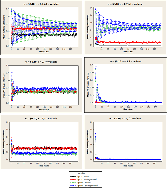
Figure A1. Mean percent grouped farmers (pg) in each time-step when price per unit is $0.10.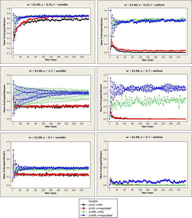

Figure A2. Mean percent grouped farmers (pg) in each time-step when price per unit is $1.00.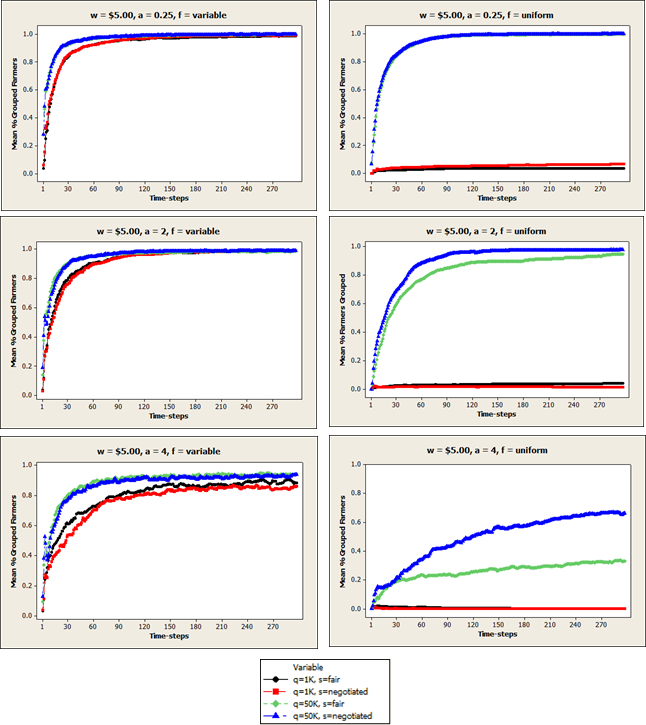

Figure A3. Mean percent grouped farmers (pg) in each time-step when price per unit is $5.00.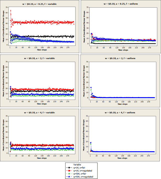

Figure A4. Mean number of coordinated farmer groups (ng) in each time-step when price per unit is $0.10.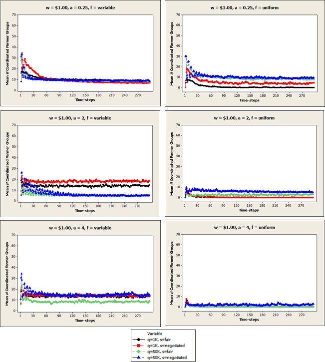

Figure A5. Mean number of coordinated farmer groups (ng) in each time-step when price per unit is $1.00.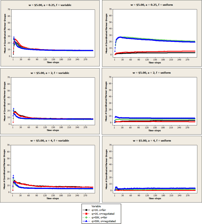

Figure A6. Mean number of coordinated farmer groups (ng) in each time-step when price per unit is $5.00.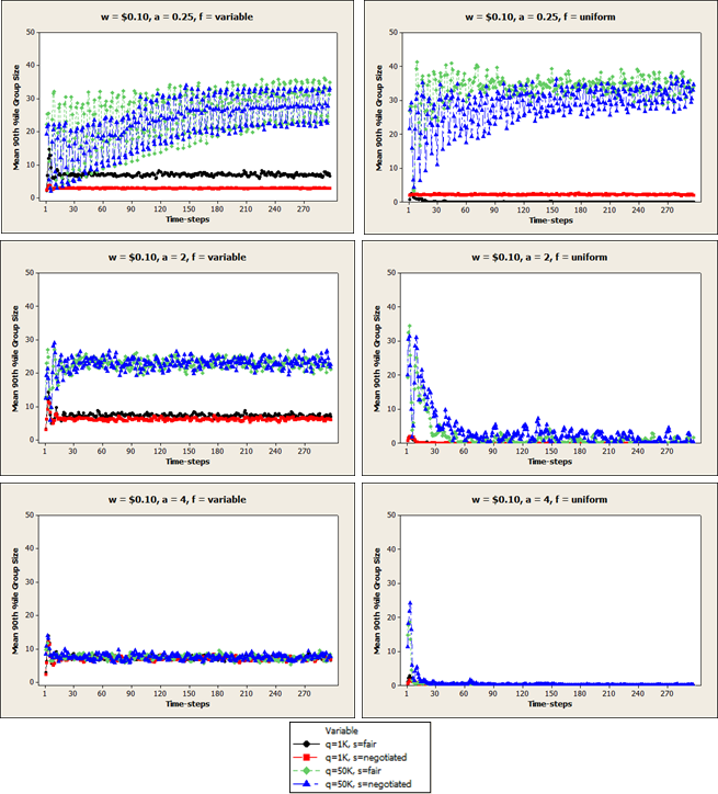

Figure A7. Mean 90th percentile farmer group size (gs) in each time-step when price per unit is $0.10.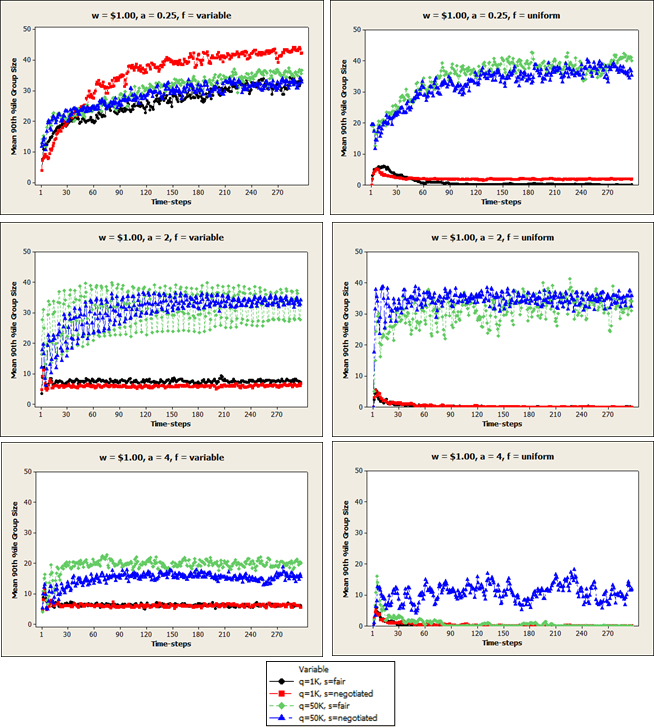

Figure A8. Mean 90th percentile farmer group size (gs) in each time-step when price per unit is $1.00.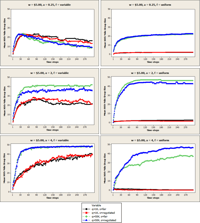

Figure A9. Mean 90th percentile farmer group size (gs) in each time-step when price per unit is $5.00.

References

AHUMADA, O. & Villalobos, J. R. (2009). Application of planning models in the agri-food supply chain: a review. European Journal of Operational Research, 196(1), 1–20. [doi:10.1016/j.ejor.2008.02.014]

DAHLBERG, K. A. (2008). Pursuing long-term food and agricultural security in the United States: decentralization, diversification, and reduction of resource intensity. In T. A. Lyson, G. W. Stevenson, and R. Welsh (Eds.), Food and the Mid-Level Farm: Renewing an Agriculture of the Middle (pp. 23–34). Cambridge, MA: MIT Press.

GARVEY, P.R. (2008). Analytical Methods for Risk Management: A Systems Engineering Perspective. Boca Raton, FL: CRC Press. [doi:10.1201/9781420011395]

GASSON, R. (1973). Goals and values of farmers. Journal of Agricultural Economics, 24(3), 521–542. [doi:10.1111/j.1477-9552.1973.tb00952.x]

GILLESPIE, J. M. & Eidman, V. R. (1998). The effect of risk and autonomy on independent hog producers' contracting decisions. Journal of Agricultural and Applied Economics, 30(1), 175–188.

GODFRAY, H. C. J., Beddington, J. R., Crute, I. R., Haddad, L., Lawrence, D., Muir, J. F., Pretty, J., Robinson, S., Thomas, S. M., & Toulmin, C. (2010). Food security: the challenge of feeding 9 billion people. Science, 327(5967), 812–818.

JANSSEN, S. & van Ittersum, M. K. (2007). Assessing farm innovations and responses to policies: a review of bio-economic farm models. Agricultural Systems, 94(3), 622–636. [doi:10.1016/j.agsy.2007.03.001]

KEY, N. (2005). How much do farmers value their independence? Agricultural Economics, 22(1), 117–126.

KIRBY, L. D., Jackson, C., & Perrett, A. S. (2007). Growing local: implications for Western North Carolina. Retrieved from http://asapconnections.org/downloads/growing-local-implications-for-western-north-carolina.pdf.

KREJCI, C. C. & Beamon, B. M. (2012). Modeling food supply chains using multi-agent simulation. In C. Laroque, J. Himmelspach, R. Pasupathy, O. Rose, & A. M. Uhrmacher (Eds.), Proceedings of the 2012 Winter Simulation Conference (pp. 1167–1178). Berlin, Germany. [doi:10.1109/wsc.2012.6465157]

LYSON, T. A. (2007). Civic agriculture and the North American food system. In C. C. Hinrichs and T. A. Lyson (Eds.), Remaking the North American Food System: Strategies for Sustainability (pp. 19–32). Lincoln, NE: University of Nebraska Press.

RENTING, H., Marsden, T. K., & Banks, J. (2003). Understanding alternative food networks: exploring the role of short food supply chains in rural development. Environment and Planning A, 35(3), 393–411. [doi:10.1068/a3510]

REYNOLDS, B. J. (1997). Decision-making in cooperatives with diverse member interests. Retrieved from http://www.rurdev.usda.gov/rbs/pub/rr155.pdf.

STAATZ, J. (1986). A game-theoretic analysis of decision-making in farmer cooperatives. In J. S. Royer (Ed.), Cooperative Theory: New Approaches (Service Report No. 18) (pp. 117–147). USDA/ACS.

WEINTRAUB, A. & Romero, C. (2006). Operations research models and the management of agricultural and forestry resources: a review and comparison. Interfaces,36(5), 446–457. [doi:10.1287/inte.1060.0222]

XU, L. & Beamon, B.M. (2006). Supply chain coordination and cooperation mechanisms: an attribute-based approach. The Journal of Supply Chain Management, 42(1), 4–12. [doi:10.1111/j.1745-493X.2006.04201002.x]