Abstract

Simulation results can be highly sensitive to the way agents are upscaled to a larger organizational and spatial level. This paper tests an ex-post validation method for forecasting models by using old base years and forecasting into recent years for which observed data is already available. Our case in point is a comparison between different upscaling methods in the agent-based agricultural sector model SWISSland. It is shown that individual-farm extrapolation factors strongly enhance alignment with the total population in the base year. However, they may cause inconsistencies in those agent-based models in which relations between the farms are an important part. Therefore, an adjustment of the sample by making almost no use of some farms whilst making highly disproportionate use of others turned out to be the most suitable method for the SWISSland model.

Keywords:

Agent-Based Model, Agriculture, FADN, Extrapolation

Introduction

1.1

The use of agent-based models (ABMs) to illustrate structural and land-use changes in agriculture is now part of the standard repertoire of agricultural economics. Starting with the pioneering models of the 1990s and at the beginning of the turn of the millennium for regions under investigation in Europe (Balmann 1996, 1997, 2000; Happe 2004), these models are now being used worldwide to find answers to agricultural- and environmental-policy issues (Bert et al. 2011; Stolniuk 2008; Lobianco & Esposti 2010; Le et al. 2012; Berger et al. 2006).

1.2

ABMs are characterised by their flexible paths in the linking of various data sources (cf. Schreinemachers & Berger 2011; An 2012; Boero & Squazzoni 2005) in order to provide a varied illustration of rational and non-rational behaviours, as well as decision-making behaviours of previously defined agents. ABMs enable a wide range of applications to be covered by taking account of numerous interactions of the agents with one another and with their environment. They are therefore used e.g. for assessing the impact of policy on various socio-economic indicators such as income distribution and structural change (Sahrbacher 2012; Freeman 2005), landscape development (Berkel & Verburg 2012), environmental impact (Schouten et al. 2013; Van der Straeten et al. 2011), climate change (Cormont et al. 2012) or potential effects on biodiversity (Polhill et al. 2012).

1.3

As in the majority of the agricultural-sector ABMs mentioned at the outset, the individual, real-world agricultural enterprise is also used in SWISSland as a template for an agent whose strategic behaviour in terms of farm growth, engaging in a sideline or production task is meant to match the behaviours observed on Swiss farms. Unlike the approaches presented, SWISSland does not focus on a single region, but rather, together with the selected sample of farms, depicts the country's entire agricultural sector. Here, advantages for policy evaluation arise primarily from the opportunity to cover the individual-farm, regional and national levels when analysing the results.

1.4

The model results for the starting year and the result trends of a projection period should square as precisely as possible with the real-life situation and the actual trends, respectively. This increases the certainty that the essential correlations in the model will be depicted. It also makes it easier for decision-makers to interpret the forecasted trends. Because the reality can never be completely depicted in a model, additional measures are required for a complete adjustment to real-life situations. At the individual-farm level, this is achieved by calibrating the farm models; at the sectoral level, via a sector-consistent extrapolation. Both calibration and extrapolation processes may, however, influence the forecasted model results. With the help of the SWISSland model, this paper investigates the effects of different extrapolation methods on the accurate depiction of the actual situation, and on the influencing of the model forecasts. Here, the main question is the extent to which SWISSland is able to depict the trends actually observed in the Swiss agricultural sector. To this end, the corresponding model results are compared with the statistical values of the agricultural sector, using various key structure and income figures. The effect of the various extrapolation methods can be measured by means of the deviation of the model results from the statistical observation values.

1.5

Section 2 of the present paper sets out a brief overview of the model itself. Section 3 aims to fill a gap in terms of the theoretical background of various extrapolation methods. Section 4 shows the influence of the different methods on the sectorally extrapolated model results.

The SWISSland Model – A short ODD Protocol

2.1

SWISSland is an empirically supported agent-based agricultural sector model developed by the Socioeconomics Research Group of Agroscope Research Station, Institute for Sustainability Sciences ISS in Tänikon, Switzerland. A number of papers describing parts of SWISSland have been published to date (Calabrese & Mack 2011; Mack et al. 2014; Mack & Hoop 2013; Mack et al. 2013; Mack et al. 2011; Möhring et al. 2012; Möhring et al. 2011; Möhring et al. 2010a and Möhring et al. 2010b). In this paper, SWISSland is described according to the ODD (Overview Design Concepts and Details) Protocol of Grimm et al. (2010).

Overview

Purpose

2.2

The SWISSland agent-based model aims to depict as realistically as possible around 55 000 family farms throughout Switzerland in all their heterogeneity in terms of operating and cost structures as well as modes of social behaviour. SWISSland is used to estimate the repercussions of agricultural policy measures, the impact of internal and external market influences, and the effects of the heterogeneous site conditions specific to the alpine region on income trends, structural change and land management in the Swiss agricultural sector. At the same time it is designed to differentiate between regional areas and groups of farms. SWISSland's primary use is as a policy advisory tool.

Entities, State variables and scales

2.3

Agents are represented by actual farms in the model. These are exclusively family farms operating all year round whose total income is generated mainly on the farm. The model also includes agents farming exclusively in the mountain region at an altitude of over 1000 m above sea level (alpine farms).

2.4

The parameterisation of the agents in terms of location, farm structure and resource endowment is based on information obtained from the approx. 3200 reference farms of the Swiss Farm Accountancy Data Network (FADN) data pool. This agent population is a non-representative sample of the approx. 55 000 family farms in Switzerland.

2.5

Located throughout Switzerland, the FADN-based agents usually have no neighbourly relationships with one other. To model land trade between these FADN-based agents, a spatially realistic municipality structure was implemented in the sector model which includes neighbourhood patterns among farm locations (Mack et al. 2013).

2.6

Agents exhibiting similar characteristics in terms of individual behavioural strategies within their adjustment process were grouped into population clusters. Population clusters exist in the spheres of work organisation and investment activity (Mack & Hoop 2013), in the depiction of generational change (Möhring et al. 2011), in the decision for or against the expansion of labour- and capital-intensive production branches of plant production, in the change of the land use system, or in the depiction of the home farms that are amenable to summering livestock (Calabrese 2012).

2.7

The market price is recalculated annually on the basis of price elasticities of demand with the help of a partial equilibrium model within two iteration steps. Integrated into the iteration process is the SWISSland demand module, which is used for ex-ante simulations. For ex-post simulations, the individual-farm prices and average sectoral price trends deduced from the FADN data are assumed. Exogenous variables predefined for the model are inter alia general macro-economic and population trends, relevant policy instruments such as threshold prices, quota controls, direct payments, benefits and import quotas as well as the world market price and all individual-farm input data. The latter may vary depending upon specifications and framework conditions motivated by agricultural policy. A general model overview is given in Figure 1.

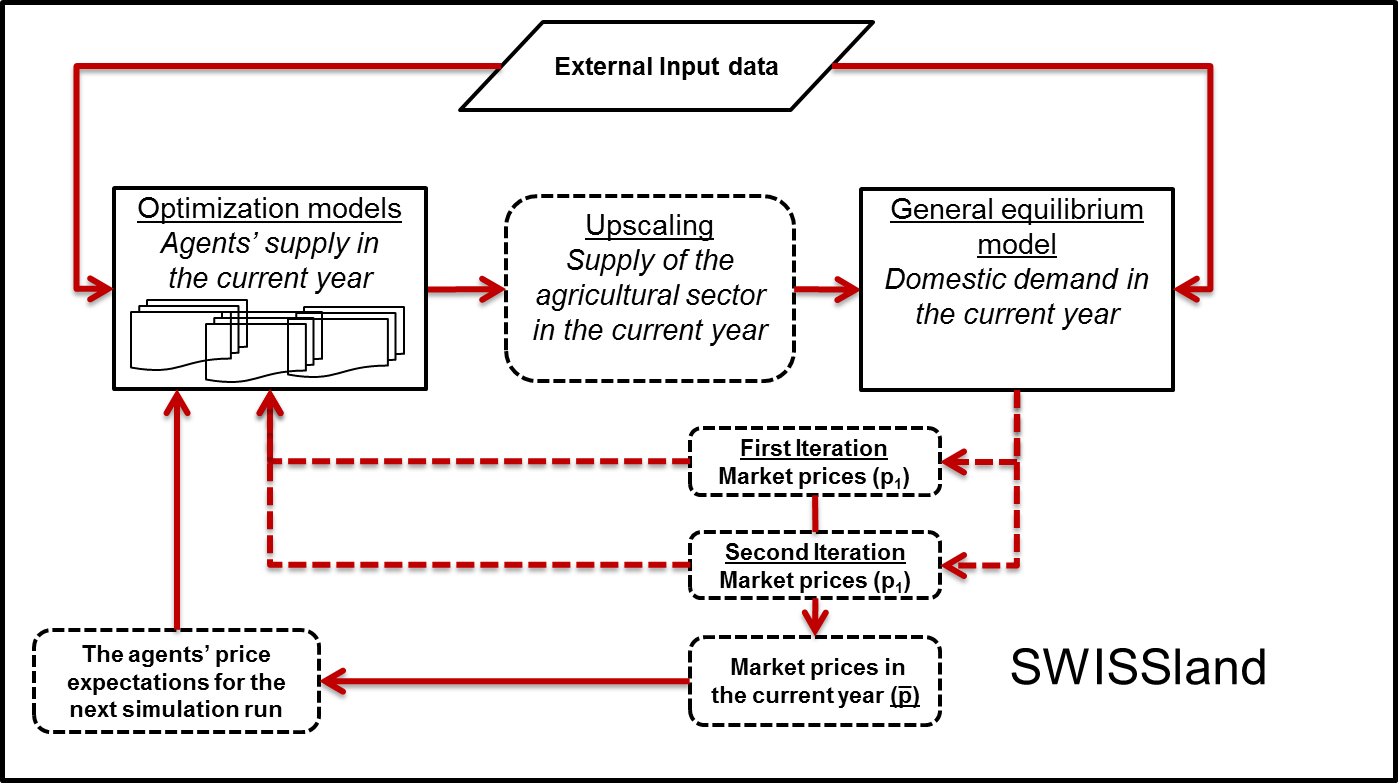
Figure 1. The model system SWISSland

Process overview and scheduling

2.8

The adaptive reactions of the individual agents are depicted in annual steps. Before the annual iteration process can be started, an initialisation step is necessary.

2.9

The initialisation process essentially consists of the following substeps:

1. Improving the representativeness of the sample
2. Importing the FADN data and other data sources
3. Parameterising the individual-farm optimisation models
4. Assigning attributes to the agents
5. Calibrating the base year
6. Assigning typical behavioural rules for individual agents or agent groups

2.10

The iteration process is then started, with the model flow depicted in Figure 2 applying for each time interval. The model simulates a forecast period of up to 30 calendar years, corresponding more or less to a generational cycle of the farming family. The adaptive reactions of the individual agents (\(A_n\)) and their behaviour when interacting with other agents are depicted in annual steps.

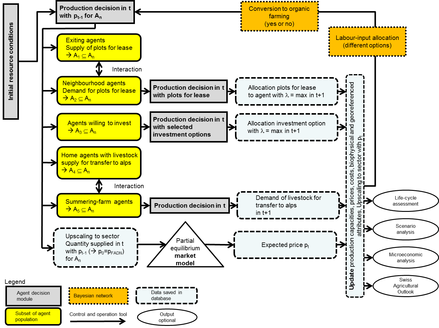
Figure 2. Design and process overview of Swissland

Software environment

2.11

SWISSland comprises three different software components which communicate with each other via interfaces:
MySQL database

• Accountancy data
• Simulation control data for process and data-transfer control
• Group-formation data for creating population clusters and SWISSland communities
• Input and output data for mapping each individual agent's behavioural algorithms in decision-making

Java platform

• Modelling database interfaces and program control
• Modelling the non-rational decision-making behaviour of agents
• Modelling agent interactions
• Modelling extrapolation across the sector as a whole

GAMS optimisation model

• Modelling farm agents with GAMS (General Algebraic Modeling System: Rosenthal 2015)
• Data preparation tool: allocation of accountancy data to production activities
• Optimisation of agents' production and investment decisions
• Calibration of the model

2.12

Many of the processes within a simulation must be handled sequentially. Except for base year data preparation in the initialisation phase, however, most individual-farm GAMS optimisations can be initialised in parallel for the total of 59 SWISSland lease regions.

Design Concepts

Basic Principles

2.13

The SWISSland model is a hybrid model. The microsimulation approach (individual-farm optimisation) investigates the rational decision-making process of the agents at microlevel.

2.14

The agent-based model approach also enables non-rational agent decision-making behaviour to be taken into account, and allows interactions between the agents themselves on the one hand, and between the agents and their environment on the other. This permits scenario- and policy-based analysis, as well as the description of structural impact on a micro- and sector level.

Emergence

2.15

The SWISSland model calculates sectoral parameters. First and foremost, these include trends in product quantity, price, land use, livestock population and workforce, as well as income trends according to agricultural accounting, sectoral input and output factors for calculating environmental impacts, and important structural indicators such as the number of farms, farm sizes and farm types, or the number of farms that have changed their form of land use.

Adaptation

2.16

The great heterogeneity of Swiss family farms and the differentiated regional and local circumstances taken into account indirectly via production resources and individual cost- and price ratios of the agents elicit different adaptive reactions. Agents can adapt their production programme, and correspondingly their use of resources (land, labour, cash and livestock) whilst bearing in mind technical progress, price changes on the product and factor markets, and agricultural-policy transfer payments. This is accomplished through a changed mix of production activities, or through the expansion or restriction of production volumes. Farm exits are possible within the framework of generational change, whilst growth occurs through the leasing of the plots of exiting agents, or through investment in larger barns.

Objectives

2.17

One of the most important assumptions of the model is that the agents maximise their expected household income, which is the sum of agricultural and non-agricultural income. For this, they optimise their (short-term) production and investment decisions.

Learning

2.18

No agent learning process is implemented in SWISSland; however, the model adapts the behavioural rules in year t₁ based on the decisions in year t.

Prediction

2.19

In keeping with the theory of adaptive expectations, the agents make their production decisions based on yield and price expectations of the previous year for the various products. In addition, annual yield increases resulting from technical progress are taken into account as well as changes in costs based on cost trends in the upstream area or in the service sector.

2.20

The agents base their investment decisions on the expected average annual costs for the entire capacity of an investment unit, regardless of whether or not it is fully utilised in the short term after the investment.

Sensing

2.21

It is assumed that the farmers are familiar with the site of their farm and that of their plots or potential neighbouring plots, and therefore bear in mind the relevant transport costs in the event of a possible leasing decision. They also know the transport costs for the transfer of the animals from the home farms to the summering farms. These costs influence the home farms' decision to summer livestock on alpine pastures.

Agent-Agent Interaction

2.22

SWISSland uses a leasing algorithm to model the allocation of plots of land from exiting farms to the remaining farms in the immediate vicinity (Mack et al. 2013). Exiting farms are those which cannot be transferred to a successor or those where potential successors decide against taking over the farm for economic reasons. A plot-by-plot bidding process is used to model which neighbouring agent obtains the freed-up land and at what rental. The plot is allocated to the neighbouring agent achieving the highest expected income growth from leasing the plot. As soon as a plot of land cannot be leased in the normal bidding process, the lease price is reduced incrementally by 20% each time the circle of prospective buyers is expanded.

2.23

Another inter-farm interaction in SWISSland takes place when summer-pastured livestock is transferred between home farm and alpine farm at the beginning and end of the summer season. If an alpine farm is privately run, the summered animals from the home farm are allocated directly to the alpine farm. If it is an alp cooperative, the livestock is assigned to alpine pastures via a so-called middleman, who allocates the available animals subject to the capacity of the summer farms and the distance, or more specifically the cost of transporting the livestock. This method of indirect interaction is also described by Bandini et al. (2009).

Agent-Environment Interaction

2.24

The agent-environment relationships are taken into account indirectly via the individual-farm parameter coefficients of the model agents. Site and climate conditions are reflected both in land use and in yield potentials and cost structures of the farms of the base year. SWISSland is linked to environmental life cycle assessment (LCA) software via an output tool so that a final environmental-impact analysis can be carried out for each simulation. Feedback to the model based on the results of the environmental LCA is not possible at the moment. Decision-making options which would allow an adaptive response from agents, e.g. a switch to particularly resource-efficient or climate-friendly cultivation methods, have not as yet been modelled.

Stochasticity

2.25

SWISSland implements stochastic variables and processes in several places:

• For all agent activities occurring in the production programme of the forecast years rather than in the base year, the yield and price coefficients are estimated with the aid of a random distribution based on means and standard deviations of the values of all agents from the same region and with the same land use system.
• The model uses a random distribution of farmer's age, which was predefined in the initialisation process. Here, the age distribution of the agent population corresponds to that of the basic population.
• The useful life of existing barns is estimated on the basis of the depreciation amount per LU, since no information on the actual age of the barns can be derived from the accounting data. Here, the assumption applies that the higher the depreciation amounts per LU, the shorter the useful life of the barn. Within a quantile allocation of the agents, the age of the barns is determined stochastically via random distribution.
• Agents without a (male or female) successor and those with a potential takeover candidate are determined stochastically on the basis of farm-succession probabilities. Probabilities are reallocated after each simulation year, so that the dynamic changes in the agents resulting from a growth in area or change in farm type are taken into account in the simulation period.

Cooperatives

2.26

SWISSland does not depict cooperative associations that have an effect on the individual agent decisions.

Observation

2.27

After each iteration, the state after the optimisation process is recorded and stored in the database. This information serves as input parameters, and hence as a decision-making basis for the next time interval. In addition to the age of the farm manager and that of the agricultural buildings, information on spatial attributes and changing behavioural traits and rules is updated. After the simulation, all relevant parameters are extrapolated at sectoral level. The adaptive reaction of the agents can be shown individually, or individually for each time interval for groups of agents, or for several or all time intervals of the entire forecast period.

Details

Initialisation and modelling of agent behaviour

2.28

The FADN-based agents are located throughout Switzerland, and do not usually have a neighbourly relationship with each other. To model land trade between agents, a spatially realistic municipality structure including neighbourhood patterns among farm locations was implemented in the model. The municipality structure was based on seven existing Swiss municipalities. The seven reference municipalities were chosen from among Switzerland's 2,765 municipalities in a two-step procedure. Firstly, a municipal typology was created on the basis of size (utilised agricultural area or UAA), difference in altitude (between the lowest and highest point above sea level of the UAA), and distribution of the farmland over different altitude levels within a municipality. These attributes were selected as indicative of accessibility and travel time between the farm locations and the plots of a municipality. Mack et al. (2013) provided details on the assignment of reference municipalities and their spatial and topographic characteristics, as well as on the information transfer process from municipality level to FADN-based agent level. Consequently, all agents were determined by spatial characteristics (farmyard coordinates, number of plots with meadows and arable land, coordinates of the plots and their field-farmyard distance), and ultimately possessed 'virtual' neighbouring agents whose plots border on other agents.

2.29

The modelling of agent behaviour fundamentally influences the manner in which the actors make their decisions. The behaviour of the individual agents can be divided into smaller independent units (microbehaviours) that are individually parameterised and modelled as autonomous processes (Kahn 2007). Initially, this occurs independently of the sequence of the execution of the processes, but must subsequently be coordinated with them:

2.30

Rational agent behaviour is taken as an important basic assumption of the model. In the objective function (equation 1), each farm agent (index \(f\)) maximises its household income per annum (index \(t\)). Household income (\(INCOME_f,t\)) is yielded from the sale of products (\(SALE_y\)), from additional income (\(ADDINC_i\)), and from income from direct payments (\(PAYMENT_d\)), less the costs of the means of production (\(PURCHASE_x\)). Almost all product and purchase prices were estimated on an individual-farm basis from the FADN data, with the price trends being stipulated exogenously. The cost function of the plant-production activities is formulated according to the approach of Positive Mathematical Programming (PMP) described in Mack et al. (2015), where different PMP methods are also tested. By taking into account additional, calculated costs (\(\alpha_c, \gamma_c\)) for the enlargement of the individual crop areas (\(LAND_c\)) in relation to the observed areas in the base year, PMP helps to obtain reactions by the agents in the model similar to those observed among farmers. For the mathematical details of this method, see Heckelei et al. (2012), Sanders et al. (2008) or Gocht et al. (2005).

2.31

The optimised activity values have to comply with various restrictions (equation 2). The resource endowment (\(w\)) of a farm consists of the available area (index \(c\)), the animal places (index \(l\)) on the home farm and the alpine farm (index \(v\)), the labour force (index \(h\)), and other capacities limiting animal and plant production (e.g. sugar-beet quota, milk quota up to 2009, provisions on the receipt of direct payments). All restrictions are in linear form in order to get an optimal solution with commonly used solvers.

$$ Max\,INCOME_{f,t} = \sum_y \rho_y \ast SALE_{f,t,y} + \sum_i \rho_i \ast ADDING_{f,t,i} + \sum_d \rho_d \ast PAYMENT_{f,t,d}- \sum_x p_x \ast PURCHASE_{f,t,x}- \sum_c \alpha_{f,c} \ast LAND_{f,t,c}- 0.5 \sum_c \gamma_{f,c} \ast LAND_{f,t,c}^2 $$

(1)

subject to

$$ \sum_c \omega_{c,w}^{LAND} \ast LAND_{f,t,c} + \sum_{l,v} \omega_{l,v,w}^{ANIMAL} \ast ANIMAL_{f,t,l,v} + \sum_h \omega_{h,w}^{LABOUR} \ast LABOUR_{f,t,h} \leq \beta_w $$

(2)

for all \(w \notin c,l,v,h\).

2.32

The use of individual-farm FADN data ensures that various factors influencing the objective function and production-coefficient matrix are also automatically taken into account, allowing the depiction of numerous management options that are typical for Switzerland. These management options are characterised by different arable-, forage- and animal-production systems within the land-use system, and thus by corresponding input/output intensity levels. The cost and output parameters of the production activities are therefore heterogeneous, and influence the decision-making scope of the agents.The coefficients derived using the base year apply only for the current situation of the agents, however.

2.33

There are so called real-world strategies implemented in the decision models of SWISSland, e.g.:

• At the earliest, farm-takeover decisions are considered once the farm manager turns 65 and starts receiving his state pension, coinciding with a lapse of entitlement to direct payments (Meier 2007).
• Empirical studies indicate that the number of farms involved in the lease market is limited (Strohm 1998), ranging between one and five farms. Based on these findings, it was assumed that the five nearest neighbours were involved in the bidding process.

2.34

Farm takeover or farm exit are determined by a minimum withdrawal of agents that reaching retirement age (exit rule). However, the subsequent generation opts only for a takeover, if a continuation of operation provides a sufficient basis of economic performance and thus financial stability. Is a takeover of the farm excluded due to the fact that the basic business requirements cannot be achieved, the land is released for lease. The implemented income and stability criteria guarantee that agricultural policy changes (including price reductions, reduction of direct payments) incorporated in the takeover decision (Figure 3).

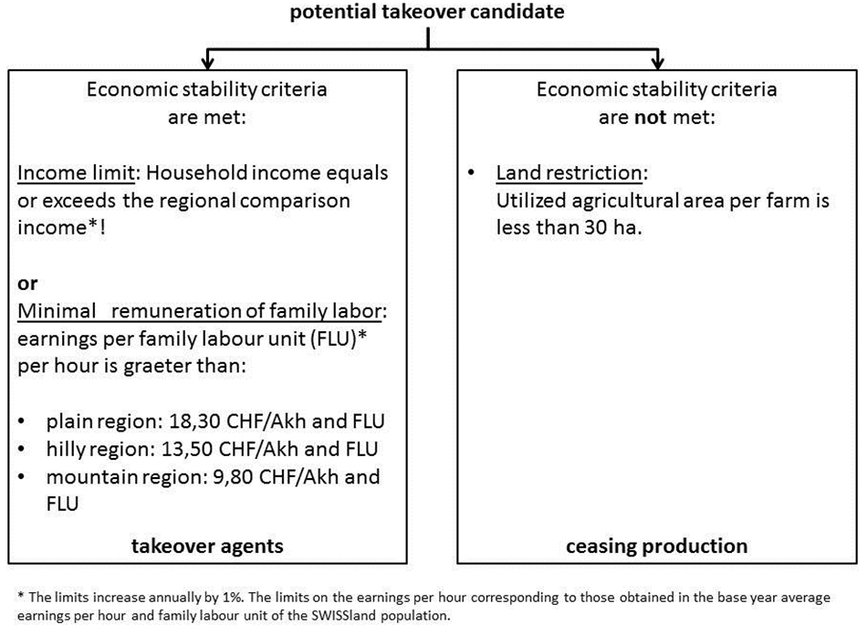
Figure 3. Economic stability criteria for farm takeover decisions

2.35

Various techniques are used in SWISSland to model types or groups of individuals with similar preferences, e.g.:

• For agents that have not yet cultivated any permanent crops in the base year, a descriptive analysis of FADN farms is used to determine farm-management and structural predictors (e.g. ha UAA, ha arable land, outside-workforce numbers, para-agriculture gross output, high equity accumulation), which limit entry into branches of permanent-crop production (vegetable/fruit production) during the simulation period.
• A cluster of FADN farms were analysed to determine the common labour strategies for Switzerland with respect to use of family labour, external labour, wage labour by a third party, wage labour for a third party and sideline with area expansion through the lease of additional land. A distinct strategy \(c_x\) is defined by the mean absolute deviation (\(d_x\)) of all five cluster-forming variables over the period \(t_1\). In addition, we describe a labour strategy \(c_x\) by a set of m underlying farm-structure variables \(S_{jx}\) from period \(t_0\) where \(j= (1\ldots m)\), representing the farm's status before the change. Farm structure differences between at least two clusters were verified by applying a Kruskal-Wallis test. A Bayesian network calculates the posterior probability distribution P(E) to a distinct cluster for each agent.

2.36

According to Kellermann et al. (2008), model-specific assumptions are necessary in order to render the model operational and to keep it tractable and clear. In particular, assumptions concern the following: data gaps, conversion, farm behaviour, expectation formation, planning-period definition, market representation, and interaction with other sectors. Central modelling assumptions are listed in Balmann (1996), Kellermann et al. (2008) and Sahrbacher (2012). Hence, the following basic economic assumptions apply for SWISSland: profit or income maximisation, lower costs and path dependency, economies of size, myopic behaviour, shadow price, transport costs, and opportunity costs.

Input and Output data

2.37

The database combines three groups of data:

• Simulation-control data (for scheduling and data transfer between modules)
• Group-formation data (for forming population clusters and SWISSland municipalities)
• Decision-making behavioural datasets for each agent.

2.38

The agents make their production decisions on the basis of yield and cost expectations of the three-year average of the production programme conducted in the base year and of the product prices of the previous year. Expected costs, direct payments and expected yields were estimated for all non-existent agent production activities of the base year by estimating averages and standard deviations of the observed values of similar farms. These groups include farms in the same regions with similar farm types. This method is especially suitable for deriving the expected values for homogeneous farm activities such as commercial milk production or cereal production, since these are recorded in detail in the individual-farm accountancy data. The correct depiction of heterogeneous farm activities (such as vegetable production) which are underrepresented in the accountancy data and whose cost- and labour-requirement coefficients are not clearly assignable, is a trickier matter. In addition, various production processes of these farm activities often vary dramatically with respect to area output in monetary terms and working-time requirement, with the result that an aggregation of various processes to an activity in the model leads to distortions. A grouping of the farms is possible if, assuming a reference gross output per hectare of area, the actually achieved gross output of each individual farm is placed in relationship to this. The reference gross output is defined so as to illustrate the maximum possible gross output per hectar of the crops produced. Based on the resultant factor, the farm is now allocated to a group. Each group represents different levels of management intensity. A low factor means low area output in monetary terms, a high factor means a correspondingly high area output. Inasmuch as cost- and work-requirement coefficients correlate with the monetary area output, we can in a further step use reference values to calculate the average working time spent or the average variable costs per unit of gross output produced for the activity in question (cf. Möhring et al. 2012).

2.39

This data source is also linked to additional but incomplete information. The spatial dimension of the model is completed with GIS data. Parameters changing over the course of time such as yield increases, cost changes, the elimination of trade barriers, or the level of transfer payments motivated by agricultural policy are predetermined exogenously.

2.40

SWISSland calculates sectoral parameters via an upscaling method as described in the following section. Product quantities and prices, land-use and labour trend, income trend according to the Economic Accounts for Agriculture, the sectoral input and output factors for calculating environmental impacts, and important key structural figures such as number of farms, sizes and types of farm, or number of farms changing their farming system, are all sectoral output indicators.

Submodels

2.41

Following the ODD protocol, this section aims at providing a full model description, especially in the form of mathematical equations. Therefore submodels are explained in greater detail in Möhring et al. (2014).

Upscaling methods tested with SWISSland

3.1

Until now, sector models have usually depicted the agricultural sector as a virtual large farm, or as subdivided into regional farms. The individual-farm, heterogeneous decisions and the inter-farm relationships cannot be taken into account in such models sufficiently, if at all. Therefore, such a subsuming of individual farms into larger units can be expected to produce sizeable aggregation errors (Brandes 1985; Table 1). When modelling similar farms as farm types or average farms, this aggregation error can be reduced (e.g. FARMIS: Bertelsmeier et al. 2003). Often, however, such a farm model is not based on the basic population of farms (because data are not available from all farms, for instance). In such cases, a sampling error arises which characterises the difference between the true values of the basic population and those of the extrapolated sample. If a random sample is not possible, the representativeness can be improved by a strategic selection of typical farms (Happe 2004). Only when all farms of the basic population are included in the model can aggregation and sampling errors be avoided.

Table 1: Possible representation errors for the entire region in various sector models
Model type		Aggregation Error	Sampling Error
Regional farms	Entire regions as virtual farms	+++	(-)
Farm types	Groups of average farms	++	+
Farm sample	Representative selection	(-)	++
	Non-representative selection	(-)	+++
	Complete coverage of the region	(-)	(-)
Source: Own research

3.2

An essential aim of the SWISSland model is to forecast structural change in Swiss agriculture. Structural change is a result of the decisions at single farm level. A multi-agent model depicting all of the approx. 50,000 farms in Switzerland would be hard to implement, however, since the necessary data are not available from all of the farms. The high volume of data and long computer run times would make application extremely difficult. For this reason, SWISSland only depicts a sample of all farms, which makes an extrapolation necessary for sectoral statements.

3.3

It is our objective to progress from the individual-farm results of a model to a regional, sectoral or structural level. Hence, a method must be developed which reflects as faithfully as possible both the reactions of the farm model and the official numbers from the statistics. This method has to be based on attributes that are available both from the individual farms and from the basic population. In Switzerland, only structural attributes such as surfaces of cultivated crops and numbers of animals are systematically collected from all farms. Economic figures are only available from the FADN farms. Table 2 shows some important structural attributes for the basic population and for the farm sample in the base year 2005. The average numbers per farm indicates that some attributes are strongly under or overrepresented. The share of small sized farms and the surfaces of permanent crops are much lower in the sample, whereas the dairy cow population is higher. The average area per farm is higher in the sample too.

Table 2: Summarised and average values of some important attributes in the population and in the sample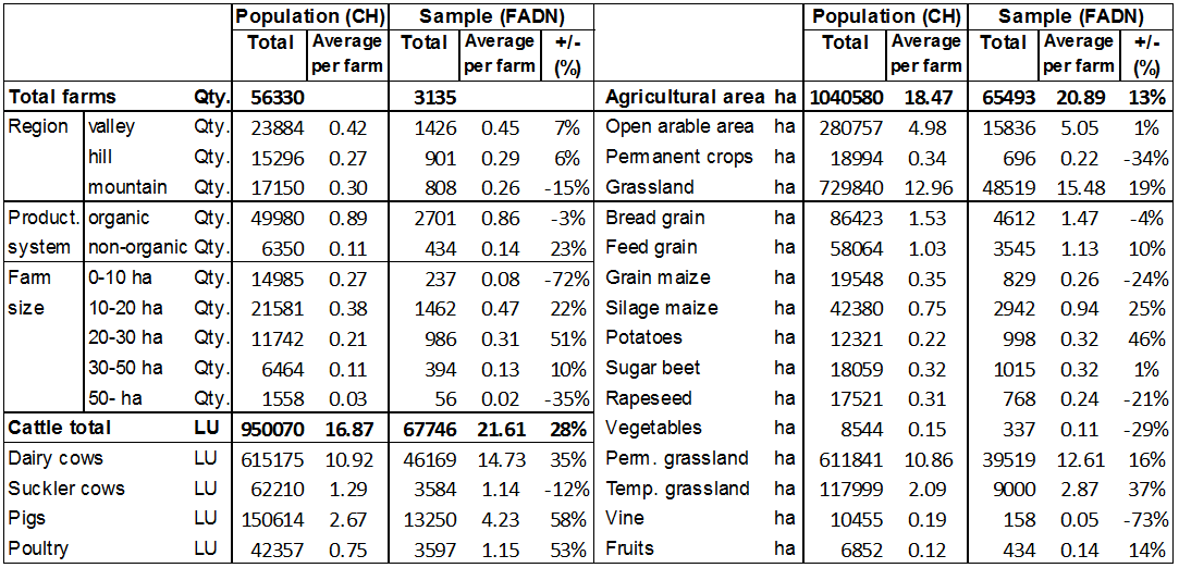

3.4

The objective of the extrapolation is to apply the results of the model that is based on the sample to the appropriate basic population using specific methods. For this, a suitable weight is generally sought for every micro-unit (individual farm) of a micro-database (sample). As a result, the sum of attributes formed in each case with these weights should correspond as closely as possible across all micro-units to the given data of the basic population. In the literature, different objective/distance functions such as generalised least squares and minimum information loss are called upon for this. In this optimisation process, the extrapolation factors can be determined either by minimising the deviations from initial extrapolation factors or by minimising the deviations from the statistical characteristics.

3.5

In multi-agent models where relationships such as land trade exist between the agents, the allocation of individual-farm extrapolation factors, however, can lead to inconsistencies in the extrapolation: Land trade between farms to which different extrapolation factors are assigned leads to a change in the stipulated total area (Fig. 4, middle). This change in area can be corrected by a corresponding adjustment of the farm extrapolation factors, i.e. the factors are adjusted such that the extrapolated total area remains unchanged (Fig. 4, right). At the same time, however, such a correction has repercussions for the extrapolation of all remaining farm attributes. The extrapolated values of attributes would change not as a result of the model calculations, but simply because of the correction of the extrapolation factors. To prevent such inconsistencies, the proxy of the farms in the agent population could be adjusted beforehand to the proxy in the basic population, based on the initialisation method of Happe (2004). Unlike in Happe (2004), however, the number of certain farms would not be multiplied until the entire region was covered. Rather, farms from under-represented farm groups would be multiplied and, if applicable, some from over-represented groups would be removed from the agent population. The goal of this adjustment is that all essential attributes are represented with a similar percentage. In this way, the results of model calculations can be extrapolated to the basic population with a general, fixed factor. The last of the extrapolation methods tested in the following section is a method using such an adjusted farm sample.

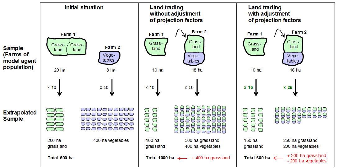
Figure 4. Aggregation errors of land trade with farm-specific extrapolation factors

3.6

The SWISSland model is used to test the suitability of different extrapolation methods for multi-agent models meant to illustrate an entire sector. For this, the methods for an earlier base year are applied, so that in addition to the accuracy of the adjustment to the population of the base year, the differences between the model results and the actual trend can be investigated. The methods contained in Table 3 are tested.

Table 3: Upscaling versions (details in the e-appendix)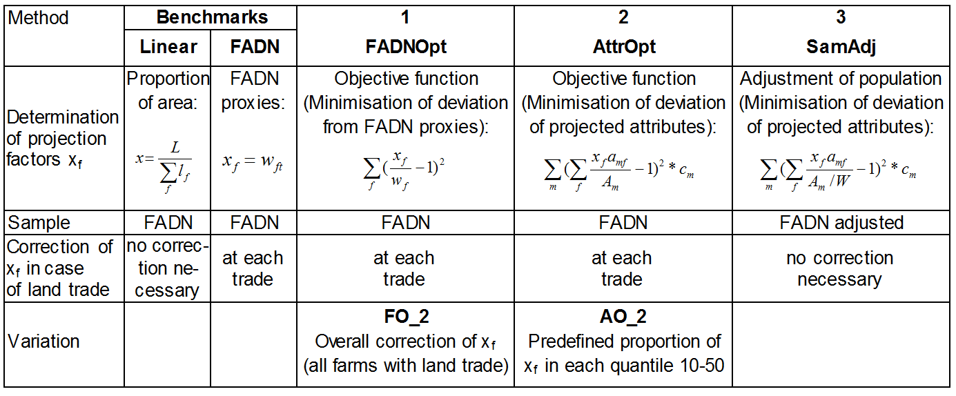

3.7

In all but the last method, the agent population of the unaltered sample corresponds to all FADN farms which were included at least twice in three consecutive years (2003-2005). For each farm, the mean values of these two or three years are transferred into the base year of the model.

Benchmarks

3.8

The 'Linear' and 'FADN' methods serve as benchmarks. In the 'Linear' method, the results of all farms with the same factor are extrapolated to the useful agricultural area of the basic population. This factor is yielded by dividing the total area of the basic population by the sum of the area of all farms in the sample. It is calculated for the base year, and remains unchanged in the forecast years. The 'FADN' method uses the proxies of the farm types for the extrapolation. In a farm sample, each farm can be assigned to a farm type, which is defined by characteristics such as proportions of specific cultures and animals, farm size and region. The weight of a farm type in the sample is determined as the inverse of the number of the farm type in the sample with reference to the number of this farm type in the basic population. During the model calculations, the factors are adjusted when land changes between different farm types, i.e. between farms with different extrapolation factors. The factor of the farm taking over land is altered in such a way that the extrapolated useful agricultural area remains unchanged.

1. FADNOpt

3.9

Farm-specific extrapolation factors could improve the adjustment of the extrapolated values. For this purpose, the deviation of the extrapolation factors from an original weighting can be minimized using an optimisation model. The squared deviations are used, in order to convert negative values into positive ones (equation 3). Alternatively, logarithmic values can be minimized (e.g. Osterburg et al. 2001). At the same time, a specific range of variation of important extrapolation attributes must be observed (equation 4). The extrapolated number of farms must remain the same (equation 5). Thus, the optimisation leads to compliance with a fixed maximum deviation \(\alpha_m\), with as little change in the original weighting factors as possible.

$$ Min Z = \sum_f \left(\frac{x_f}{w_{ft}}-1 \right)^2 $$

(3)

$$ (1-\alpha_m) \ast A_m \leq \sum_f x_f \ast a_{mf} \leq (1+\alpha_m) \ast A_m $$

(4)

$$ \sum_f x_f = \sum_{ft} w_{ft} $$

(5)

\(w_{ft}\) Basic weight of farm type \(ft\) in the sample
\(x_f\) Optimised extrapolation factor for farm \(f\) (every farm \(f\) is assigned to a farm type \(ft\))
\(\alpha_m\) Maximum permitted percentage deviation of the extrapolated attributes \(a_m\) from the range of attributes in the basic population \(A_m\)
\(A_m\) Value of attribute \(m\) in the basic population
\(a_{mf}\) Value of attribute \(m\) on farm \(f\)

3.10

The weight wft is the original weighting of the farm types ('FADN' proxies). It is the same for all farms \(f\) belonging to the same farm type, whereas the optimised factors \(x_f\) are farm-specific. Narrower permitted ranges \(\alpha_m\) are stipulated for especially important attributes such as farm numbers and areas per region than for less important ones such as single crop and livestock values. Some attributes such as the number of sheep farms are so strongly under-represented in the sample that a higher range of variation is also allowed; otherwise, very high extrapolation factors would be allocated to these few farms, with the result that a small number of individual farms would have a major impact on the model calculations. As in the 'FADN' method, the factors are adjusted during the model calculations when land is exchanged between the farms. In order to lessen distortions from these factor adjustments, the 'FO_2' method variation does not make adjustments each time that land changes hands, but rather after every model period as a whole. Here, the extrapolation factor of all farms that have taken over land during the period in question is altered by the same percentage, so that the area as a whole remains unchanged. Usually farms with low as well as with high extrapolation factors take over land,which means that some individual-farm factors are adjusted upwards and others downwards. Therefore an overall adjustment leads to smaller factor alterations, and hence to smaller distortions.

2. AttrOpt

3.11

Instead of the deviations of the extrapolation factors from an original weighting, the deviations of important characteristics can be minimised directly. Extrapolated with the farm attributes \(a_{mf}\), the to-be-determined extrapolation factors \(x_f\) are meant to deviate as little as possible from the actual attributes \(A_m\) of the basic population (equation 6). It is possible to weight the attributes in the optimisation differently (\(c_m\)). Optionally, maximum deviations for important attributes can be demanded (equation 4). Again, the extrapolated number of farms must remain the same (equation 5).

$$ Min Z = \sum_m \left( \sum_f \frac{x_f a_{mf}}{A_m}-1 \right)^2 \ast c_m $$

(6)

\(x_f\) Optimised extrapolation factor for farm \(f\)
\(A_m\) Value of attributes in the basic population
\(a_{mf}\) Value of attribute \(m\) on farm \(f\)
\(c_m\) Weight of attribute \(m\) in the objective function

3.12

In most cases the optimisation will lead either to very high or very low individual-farm extrapolation factors. Therefore, the permissible value range of the factors is limited (10 to 50). To prevent the allocation of many low or high factors within this range, the 'AO_2' method variation also defines quantiles within which certain percentages of the factors must lie.

3. SamAdj

3.13

In order to prevent distortions in factor adjustments during land trade, no different individual-farm extrapolation factors are determined in the final 'SamAdj' process. Rather, through the multiplication of farms with under-represented attributes, the agent population is adjusted such that extrapolation can be performed with an extrapolation factor that is identical for all farms. In order to detect the farms to be multiplied (\(x_f > 1\)), the deviation of the extrapolated attributes from the attributes of the basic population is minimized (equation 7). The number of farms in the agent population is given through the predefined extrapolation factor (W; equation 8).

$$ Min Z = \sum_m \left( \sum_f \frac{x_f \ast a_{mf}}{A_m/W}-1 \right)^2 \ast c_m $$

(7)

$$ \sum_f x_f = X/W $$

(8)

\(x_f\) Optimised weight of farm \(f\) (integer variable: standard value = 1)
\(a_{mf}\) Range of attribute \(m\) on farm \(f\)
\(A_m\) Range of attribute \(m\) in the basic population
\(X\) No. of farms in the basic population
\(W\) Fixed extrapolation factor: defines the percentage of the basic population depicted in the model
\(c_m\) Weight of attribute \(m\) in the objective function

3.14

Within a further equation, the maximum number of times that a farm can be multiplied (maximum of \(x_f\)) is defined. This number is set to three in this calculation. Additionally, a predefined maximum number of strongly over-represented farms may are rejected from the sample (\(x_f = 0\)). This maximum number should be small in order to limit the associated loss of information. For important attributes it is possible again to determine maximum deviations that must be observed within this optimisation process (equation 4).

3.15

Further upscaling options such as Maximum Entropy methods or the use of relative changes of attributes (Hofreither et al. 2005) have not been tested in this analysis. The latter has several drawbacks, such as all attributes must be known both of the sample and the basic population, or aggregation errors of relative changes. The effects of the extrapolation methods tested in this analysis on the extrapolation results are illustrated in the next section.

Results

4.1

The effects of the various extrapolation methods on the adjustment to the basic population in the base year and on the trend of the model results in comparison with the actual trend are illustrated below. The sample encompasses 3200 farms, thus covering 5.5% of Switzerland's farms, or 6.3% of the country's agricultural area.

4.2

Table 4 shows the deviations of the extrapolated values from those of the basic population in the base year for a range of attributes. The figures of the farm sample are model results which means that a shift from economically less to more attractive activities may have occured. These results have been extrapolated with the different methods tested. A linear extrapolation of all farms to the size of Switzerland's useful agricultural area ('Linear') leads in some cases to high deviations for various attributes. The total number of farms in the extrapolated sample is 12% lower than in the basic population. This means that, on average, the farms of the sample have a larger area than those of the basic population. Consequently, only around one-quarter of the area class of farms up to 10 ha is represented in the sample. At the same time, the farms of very large area are also under-represented. Of the various farming activities, grapes, cereals and pigs are under-represented, whilst potatoes, dairy cows and poultry are over-represented. With the linear extrapolation, the mean absolute deviation of these selected attributes is 20.7%. If the farms are not all extrapolated with the same factor, but instead according to the proxy of their farm type ('FADN'), this alone results in a distinct improvement in the adjustment. Neverthess, the small-scale farms are still underestimated in the extrapolation. For some attributes, there is even a worsening of adjustment, as is the case, for example, of the pig population, which is to be found in the sample primarily on over-represented 'combined' farm types, while specialised farms with very high pig populations are a rarity in the sample. All in all, the mean absolute deviation of the selected attributes still stands at 14%. The 'FADNOpt' method refined the farm-type-specific extrapolation factors by assigning each farm in the sample a separate factor deviating as little as possible from the farm-type-specific factor, while specifying maximum deviations from important extrapolated attributes. Thus, for instance, the very-small-scale farms can be allocated factors that are higher than the farm-type-specific factor in each case, once again enabling the extrapolation in the base year to be significantly improved, with the mean absolute deviation still standing at a total of 6.4%. The 'FO_2' method differs from the 'FADNOpt' method only in its correction process for land shifts; the extrapolation factors in the base year are identical. If the deviations of the extrapolated attributes are directly minimised ('AttrOpt') in order to determine the individual-farm extrapolation factors, the deviation rises again for several attributes, with the mean deviation reaching 8.3%. With this variant, the permitted minimum and maximum individual-farm factors were set to the narrower range of 10 to 50, since these boundary values were determined by the optimisation for a majority of the farms. In the case of land shifts between model farms, this prevents the occurrence of very high differences in the extrapolation factors, with corresponding distortions. Setting the minimum and maximum factors in this variant to 5 and 100 respectively would yield a better adjustment of attributes than in the 'FADNOpt' variant; here, however, the majority of factors would actually come to rest at either 5 or 100. In order to prevent this, the 'AO_2' method specified that a certain percentage of the extrapolation factors in each case must lie within the quartiles of the the '10 to 50' range. This additional limitation leads to a slightly worse attribute adjustment than the 'AttrOpt' method. Finally, unlike in the remaining methods, the 'SamAdj' method adjusted the agent population with respect to the sample by allowing under-represented farms to be doubled or tripled, so that a linear extrapolation by a single factor is then possible. This multiplication of individual farms offers less scope for adjustment than the individual-farm adjustment of the extrapolation factors, which is why the adjustment to the base year can be only slightly improved with respect to the linear extrapolation.

Table 4: Deviation of selected attributes extrapolated by different methods in the base year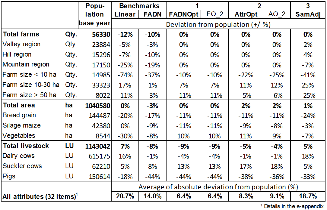

4.3

Table 5 shows how precisely the various extrapolation methods determine the actual trend of the selected attributes from 2005 to 2010. The first column gives the actual trends of the attributes as a percentage, whilst the following columns show the differences between the trend with the extrapolation method in question, and the actual trend. Thus, for example, the actual 8% decrease in farm numbers is predicted almost exactly for all methods except the last one, in which the decrease is around 5% and is therefore 3 percentage points higher. The differences arising between the methods show that the chosen extrapolation method can influence the sectoral results of the model results identical to those of the individual farm. On average for the selected attributes, the differences between the methods, i.e. the differences between the highest and lowest attribute trend, come to about 75% of the actual trends. The lowest on average are the deviations from the actual trends in the case of the last extrapolation method, although the latter did a poorer job of illustrating the basic population in the base year than did the method with extrapolation factors for the individual farm. The risk of distortion effects from the extrapolation factors for the individual farm can be highlighted using the example of farms from the area class of up to 10 ha: At around 25%, this farm group is strongly under-represented in the sample vis-à-vis the basic population. The small-scale farms are particularly at risk of exit. When they are only present in the agent population in small numbers, exit pressure on these farms increases, causing the percentage of exiting farms in this group to be overestimated. In the extrapolation, this percentage increases still further owing to the higher extrapolation factors of these farms. The actual trend for the number of farms in this group shows a 17% decrease for the period under observation. In the methods with extrapolation factors for the individual farms, this decrease is overestimated by up to 12 percentage points. By contrast, the 'SamAdj' method gave rise to a prior adaptation of the sample, thanks to which the under-representation of this group was significantly reduced. In the model calculations, this led to a lower exit rate for this farm group.

Table 5: Actual deviation of selected attributes in the forecast extrapolated by different methods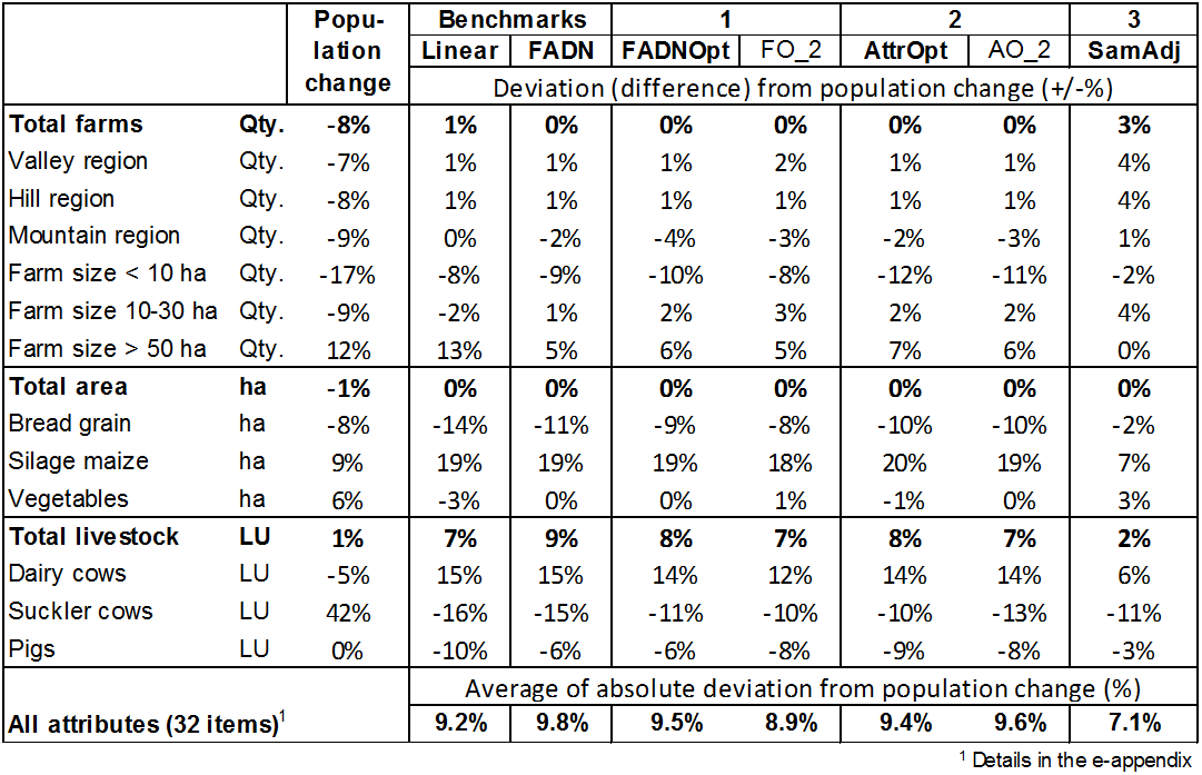

4.4

A second distortion effect in the case of individual-farm extrapolation factors results from the adjustment of the factors where land is traded between two farms with different factors. A comparison to an extrapolation without such a factor adjustment (not presented in table 5) shows that this alters the forecasted trend of the attributes by an average of about 10%; for less frequent attributes this change can be substantially higher. With the method where the factors are adjusted as a whole ('FO_2'), rather than after each land trade, this effect is reduced to around one-third.

4.5

All in all, the comparison of the various extrapolation factors shows that the choice of method can strongly influence the model results. Although extrapolation factors for the individual farm can help to achieve better alignment with the attributes in the base year than can an adjustment of the agent population via the multiplication of under-represented farms, a sample which strongly deviates from reality can influence model behaviour here. The adjustment of the individual-farm extrapolation factors also has a distortion effect during land trade, but these factors can be significantly reduced by an adjustment for the entire agent population instead of one for each individual land trade. When choosing the extrapolation method, these circumstances should also be borne in mind.

Conclusions

5.1

The lessons drawn from the analysis described above can be grouped into two categories: those drawn for improving the SWISSland model, and those drawn from a purely methodological perspective. Starting with the second category, it has been shown that it can be helpful to apply optimisation models in such a way as to allow comparison with observed developments. This is probably the only manner of comparing different methodological options which are all theoretically plausible in a normative fashion. Furthermore, a validation process in which different options are analysed has a positive influence on the reliability of the model results. On the other hand, it has to be conceded that methods that have been working well in the past (as shown by ex-post calibration) do not necessarily work well in the future.

5.2

As is probably the case for most FADN networks, the Swiss FADN does not constitute a representative sample of Swiss agriculture. When it is used as the main data source for a forecasting model, this fact should always be borne in mind. It has been shown that the best results are obtained from the SWISSland model if it is allowed to use a certain group of farms more than other groups. An adjustment of the sample, by a multiplication of under-represented farms and a removal of over-represented farms, showed a better alignment with the observed trends, and it prevents inconsistencies caused by relations between farm agents to which different extrapolation factors have been assigned. On the other hand, an optimisation of individual-farm extrapolation factors could help to enhance alignment with the total population. Furthermore, research is needed to verify which method is most appropriate in cases of bigger changes in economic or political conditions within the time period under consideration. As every model is different concerning structure, data base and objectives, the most suitable method for the extrapolation on the sector probably has to be determined for every model separately. The sensitivity of the model to the aggregation approach, and the lack of any clear 'winner' in terms of which approach should be taken suggests that agent-based models with 'aggregated agents' is, if not something that is fundamentally flawed (e.g. because individual-agent interactions such as land exchange are problematic to represent), at least an area that needs a huge amount of work.

References

AN, L. (2012). Modeling human decisions in coupled human and natural systems: Review of agent-based models. Ecological Modelling, 229(0), 25-36. [doi:10.1016/j.ecolmodel.2011.07.010]

BALMANN, A. (1996). Druck, Sog und die Einkommenssituation in der westdeutschen Landwirtschaft. Berichte über Landwirtschaft 74(4), 497–513.

BALMANN, A. (1997). Farm-based Modeling of Regional Structural Change. European Review of Agricultural Economics, 24(1), 85–108. [doi:10.1093/erae/24.1.85]

BALMANN, A. (2000). Modeling Land Use with Multi-Agent Systems. Perspectives for the Analysis of Agricultural Policies. Proceedings of the IIFET 2000: Microbehavior and Macroresults.

BANDINI, S., Manzoni, S. & Vizzari, G. (2009). Agent Based Modeling and Simulation: An Informatics Perspective. Journal of Artificial Societies and Social Simulation, 12(4), 4 (pp. A51–A66) https://www.jasss.org/12/4/4.html.

BERGER, T., Schreinemachers, P. & Woelcke, J. (2006). Multi-Agent Simulation for the Targeting of Development Policies in Less-Favored Areas. Agricultural Systems, 88, 28–43. [doi:10.1016/j.agsy.2005.06.002]

BERKEL, D.B. & Verburg, P.H. (2012). Combining exploratory scenarios and participatory backcasting: using an agent-based model in participatory policy design for a multi-functional landscape. Landscape Ecology, 27(5), 641–658. [doi:10.1007/s10980-012-9730-7]

BERT, F.E., Podestá, G.P., Rovere, S.L., Menéndez, Á.N., North, M., Tatara, E., Laciana, C.E., Weber, E. & Toranzo, F.R. (2011). An agent based model to simulate structural and land use changes in agricultural systems of the Argentine Pampas. Ecological Modelling, 222(19), 3486–3499. [doi:10.1016/j.ecolmodel.2011.08.007]

BERTELSMEIER, M., Kleinhanss, W. & Offermann F. (2003). Aufbau und Anwendung des FAL-Modellverbunds für die Politikberatung. Agrarwirtschaft 52 (2003), Heft 4, 175–184.

BOERO, R. & Squazzoni, F. (2005). Does Empirical Embeddedness Matter? Methodological Issues on Agent-Based Models for Analytical Social Science. Journal of Artificial Societies and Social Simulation, 8(4), 6 https://www.jasss.org/8/4/6.html.

BRANDES, W. (1985). Über die Grenzen der Schreibtisch-Ökonomie. Mohr. Tübingen.

CALABRESE, C. (2012). Evaluation of Political control Instruments for sustainable development of the swiss alpine regions and analysis of the labor market. Diss. ETH Zurich No. 20512.

CALABRESE, C. & Mack, G. (2011). Evaluation of political control instruments for the Swiss alpine region. 122nd EAAE Seminar: Evidence-Based Agricultural and Rural Policy Making: Methodological and Empirical Challenges of Policy Evaluation. Ancona, February 17–18.

CORMONT, A., Franke, J., Kuhlman, T., Polman, N., Schouten, M., van Teeffelen, A., Verwaart, T. & Westerhof, E. (2012). Dairy Farming and Newt Habitat: How Shocks in Milk Prices Influence the Optimal Design of Water Retention Policies. In: I.E.M.A.S.S. (IEMSS), International Congress on Environmental Modelling and Software, Managing Resources of a Limited Planet, Leipzig, Germany.

FREEMAN, T.R. (2005). From the Ground up: An Agent-Based Model of Regional Structural Change. Dissertation, Department of Agricultural Economics, University of Saskatchewan.

GOCHT, A. (2005). Assessment of simulation behavior of different mathematical programming approaches. 89th EAAE Seminar: Modeling Agricultural Policies: State of the Art and new Challenges. Parma, February 3–5.

GRIMM, V., Berger, U., DeAngelis, D.L., Polhill, J.G., Giske, J. & Railsback, S.F. (2010). The ODD protocol: A review and first update. Ecological Modelling, 221(23), 2760–2768. [doi:10.1016/j.ecolmodel.2010.08.019]

HAPPE, K. (2004). Agricultural policies and farm structures. Agent-based modelling and application to EU-policy reform. Dissertation, Institute of Agricultural Development in Central and Eastern Europe (IAMO).

HECKELEI, T., Britz, W. & Zhang, Y. (2012). Positive Mathematical Programming Approaches – Recent Developments in Literature and Applied Modelling. Bio-based and Applied Economics 1(1), 109–124.

HOFREITHER, M., Kniepert, M., Morawetz, U., Schmid, E. & Weiss, F. (2005). Ein regionalisiertes Produktions- und Einkommenssimulationsmodell für den österreichischen Agrarsektor. Forschungsprojekt Nr. 1319 im Auftrag des BMLFUW, University of Natural Resources and Applied Life Sciences, Vienna.

KAHN, K. (2007). Comparing Multi-Agent Models Composed from Micro-Behaviours. In: Rouchier, J., Cioffi-Revilla, C., Polhill, G. & Takadama, K. (eds.). M2M 2007: Third International Model-to-Model Workshop. Marseille, France, 165–177.

KELLERMANN, K., Happe, K., Sahrbacher, C. & Brady, M. (2008). AgriPoliS 2.0 - Documentation of the extended model. Working paper series of the European research project: The Impact of Decoupling and Modulation in the Enlarged Union: A sectoral and farm level assessment (IDEMA).

LE, Q.B., Seidl, R. & Scholz, R.W. (2012). Feedback loops and types of adaptation in the modelling of land-use decisions in an agent-based simulation. Environmental Modelling & Software, 27–28, 83–96. [doi:10.1016/j.envsoft.2011.09.002]

LOBIANCO, A. & Esposti, R. (2010). The Regional Multi-Agent Simulator (RegMAS): An open-source spatially explicit model to assess the impact of agricultural policies. Computers and Electronics in Agriculture, 72(1), 14–26. [doi:10.1016/j.compag.2010.02.006]

MACK, G., Möhring, A., Ferjani, A., Zimmermann, A. & Mann, S. (2013). Transfer of entitlements for single farm payments within farm succession. Impact on structural change and on rental prices in Switzerland. Bio-based and Applied Economics.

MACK, G., Möhring, A., Ferjani, A., Zimmermann, A., Gennaio, M.-P. & Mann, S. (2011). Farm entry policy and its impact on structural change analysed by an agent-based sector model. EAAE 2011 Congress: Change and Uncertainty Challenges for Agriculture, Food and Natural Resources. August 30 – September 2, ETH Zurich.

MACK. G., Möhring, A., Ferjani, A., Zimmermann, A. & Mann, S. (2015). How did farmers act? An ex-post validation of normative and positive mathematical programming for an agent-based sector model. Paper presented at the 29th IAAE-Conference: "Agriculture in an interconnected world", 08.-14.08.2015, Milan.

MACK, G., & Hoop, D. (2013). Modeling of structural change related shifts in labor input in the agent-based sector model SWISSland. Yearbook of Socioeconomics in Agriculture. YSA 2013. 177–199.

MEIER, B. (2007). Altersstruktur und Strukturwandel in der schweizerischen Landwirtschaft. In: BEMEPRO (ed.) Studie im Auftrag des Bundesamtes für Landwirtschaft. Winterthur.

MÖHRING, A., Zimmermann, A., Mack, G., Mann, S., Ferjani, A. & Gennaio, M. P. (2010). Modelling structural change in the agricultural sector - an agent-based approach using FADN data from individual farms. 114th EAAE Seminar: Structural Change in Agriculture. Berlin, Germany.

MÖHRING, A., Mack, G., Zimmermann, A., Gennaio, M.P., Mann, S. & Ferjani, A. (2011). Modellierung von Hofübernahme- und Hofaufgabeentscheidungen in agentenbasierten Modellen. Yearbook of Socioeconomics in Agriculture. YSA 2011. 163–188.

MÖHRING, A., Mack, G., & Willersinn, C. (2012). Gemüseanbau – Modellierung der Heterogenität und Intensität. Agrarforschung Schweiz, 3, (7-8), 382–389.

MÖHRING, A., Mack, G., Ferjani, A., Zimmermann, A. & Mann, S. (2014). SWISSland – ODD Protocol. Institute for Sustainability Sciensces ISS, Agroscope, Ettenhausen, Schweiz. http://www.swissland.org.

MÖHRING, A., Mack, G., Zimmermann, A., Mack, G., Mann, S., Ferjani, A., & Gennaio, M. P. (2010a). Multidisziplinäre Agentendefinitionen für Optimierungsmodelle. Schriften der Gesellschaft für Wirtschafts- und Sozialwissenschaften des Landbaues e.V.. 45, 329-340.

MÖHRING, A., Mack, G., Zimmermann, A., Mack, G., Mann, S., Ferjani, A., & Gennaio, M. P. (2010b). Modelling structural change in the agricultural sector - an agent-based approach using FADN data from individual farms. Paper presented at the 114th EAAE Seminar "Structural Change in Agriculture". Berlin, Germany.

OSTERBURG, B., Offermann, F. & Kleinhanss, W. (2001). A sector consistent farm group model for German agriculture. Proceedings of the 65^th EAAE-Seminar, Bonn, Germany, March 29–31, 2000, 152–159.

POLHILL, J.G., Gimona, A. & Gotts, N. (2012). Nonlinearities in biodiversity incentive schemes: A study using an integrated agent-based and metacommunity model. Environmental Modelling and Software, 45, 74–91.

ROSENTHAL, R.E. (2015). GAMS: A User's Guide. GAMS Development Corporation, Washington, DC, USA. http://www.gams.com.

SAHRBACHER, A. (2012). Impacts of CAP reforms on farm structures and performance disparities: An agent-based approach. Dissertation, Leibniz Institute of Agricultural Development in Central and Eastern Europe (IAMO).

SANDERS, J., Stolze, M. & Offermann, F. (2008). Das Schweizer Agrarsektormodell CH-FARMIS. Agrarforschung, 15, 138–143.

SCHOUTEN, M., Opdam, P., Polman, N. & Westerhof, E. (2013). Resilience-based governance in rural landscapes: Experiments with agri-environment schemes using a spatially explicit agent-based model. Land Use Policy, 30(1), 934–943. [doi:10.1016/j.landusepol.2012.06.008]

SCHREINEMACHERS, P. & Berger, T. (2011). An agent-based simulation model of human–environment interactions in agricultural systems. Environmental Modelling and Software, 26(7), 845–859. [doi:10.1016/j.envsoft.2011.02.004]

STOLNIUK, P.C. (2008). An Agent-based Simulation Approach to Forecast Long-Run Structural Change in the Saskatchewan Grain and Livestock Sectors. M.Sc., University of Saskatchewan.

STROHM, R. (1998). Verlaufsformen der Faktormobilität im Agrarstrukturwandel ländlicher Regionen. Eine empirische Studie am Beispiel von Betriebsaufgaben in den Kreisen Emsland und Werra-Meissner. University of Göttingen.

VAN DER STRAETEN, B. Buysse, J., Nolte, S., Lauwers, L., Claeys, D. & Van Huylenbroeck, G. (2011). Markets of concentration permits: The case of manure policy. Ecological Economics, 70(11), 2098–2104. [doi:10.1016/j.ecolecon.2011.06.007]