
 Abstract
- Aggression and other acute harms experienced in the night-time economy are topics of significant public health concern. Although policies to minimise these harms are frequently proposed, there is often little evidence available to support their effectiveness. In particular, indirect and displacement effects are rarely measured. This paper describes a proof-of-concept agent-based model ‘SimDrink’, built in NetLogo, which simulates a population of 18-25 year old heavy alcohol drinkers on a night out in Melbourne to provide a means for conducting policy experiments to inform policy decisions. The model includes demographic, setting and situational-behavioural heterogeneity and is able to capture any unintended consequences of policy changes. It consists of individuals and their friendship groups moving between private, public-commercial (e.g. nightclub) and public-niche (e.g. bar, pub) venues while tracking their alcohol consumption, spending and whether or not they experience consumption-related harms (i.e. drink too much), are involved in verbal violence, or have difficulty getting home. When compared to available literature, the model can reproduce current estimates for the prevalence of verbal violence experienced by this population on a single night out, and produce realistic values for the prevalence of consumption-related and transport-related harms. Outputs are robust to variations in underlying parameters. Further work with policy makers is required to identify several specific proposed harm reduction interventions that can be virtually implemented and compared. This will allow evidence based decisions to be made and will help to ensure any interventions have their intended effects.
- Keywords:
- Agent-Based Model, NetLogo, Alcohol, Night-Time Economy, Heavy Drinking, SimDrink
Introduction
-
- 1.1
- Aggression and other acute harms experienced by young adults in the night-time economy are topics of significant public health concern (Australian Institute of Health and Welfare 2013). Although policies to minimise these harms are frequently proposed, there is often little evidence available to support their effectiveness (Miller et al. 2015). This is partly due to the characteristics of Australia's drinking culture (Room 1988), which reduces the applicability of evidence from many international studies or policy evaluations. Australian evidence for the impact of policies in this area is largely based on natural experiments, where researchers have evaluated the impact of policies after they have been implemented (Kypri et al. 2011; Livingston 2008). This is critical work, but is only useful for post-hoc policy evaluations. In contrast, simulation models provide a means for assessing the likely impact of otherwise untested policies (Dray et al. 2012).
-
- 1.2
- An overarching difficulty in testing and comparing night-time economy related policies is that the same policy can affect different settings in different ways. For example, although increases in on-licence alcohol prices can lead to people consuming less in these settings, this is offset to some extent by substitution of drinking in public venues for drinking in private venues (Meier et al. 2010) or people drinking at private venues before going out to save money (MacLean & Callinan 2013; Miller et al. 2013). These indirect effects are associated with a different set of harms and need to be weighed against any benefits. Policies can also address specific types of harm that are more prevalent in particular settings. For example, being stranded in the central business district (CBD) after public transport has finished is less likely for those attending private drinking settings. One consequence of setting heterogeneity and interaction is that any model testing policy changes or combinations of changes needs to consider indirect and displacement effects, and should ideally include multiple settings.
- 1.3
- Changes in the night-time economy have different effects upon people of different income, socioeconomic background, geographic place of residence, gender and so on (Hart 2015; Meier et al. 2010). Many policy changes may have a greater effect on a subset of the population; for example changes to alcohol pricing will have more affect upon those with less money, and changes to transport options will have more effect on those who live further away from where they drink (Callinan et al. 2015; MacLean et al. 2013; MacLean & Moore 2014). Models that do not affect individuals differently are prone to error if the results are extrapolated, since they do not properly account for the dilution of effects across the entire population.
- 1.4
- Typical models used to test alcohol policy options often inadequately capture these differences in population and setting characteristics. In particular, most modelling involves little consideration of important variables such as drinking setting and context that are known to impact consumption (Callinan et al. 2014). One way to address this issue is to use agent-based models (ABMs). ABMs use a set of autonomous 'agents' to represent a population and offer a powerful and more complex method for describing human behaviour and local interaction (Gilbert 2008). Agents follow simple behavioural rules and make decisions about how to interact with each other and their environment. Using ABMs, policies can be implemented that only effect the decisions of agents at particular times and in particular settings. Large scale patterns can then emerge from a multitude of local, stochastic interactions. Further, multiple settings and agents with different characteristics can be implemented together, providing a more realistic implementation in a larger environment.
- 1.5
- Using ABMs to address public health policy questions is not new; for example, these types of models have provided great insights into infectious disease transmission (Castiglione et al. 2007; Kretzschmar & Wiessing 1998; Rolls et al. 2013) and illicit drug use (Dray et al. 2008; Dray et al. 2012; Galea et al. 2009; Moore et al. 2009). In the context of alcohol use, ABMs have been useful in understanding the influence of social networks on levels of consumption, for example in estimating both how social networks can be used to predict heavy drinking behaviours (Mercken et al. 2015; Ormerod & Wiltshire 2009), and how heavy drinkers promote increased drinking through their social networks (Giabbanelli & Crutzen 2013; Gorman et al. 2006). On a population level, the Organisation for Economic Co-operation and Development (OECD) recently used similar simulation modelling techniques to estimate the economic and public health benefits of reduced alcohol consumption (Cecchini & Sassi 2015; OECD 2015), finding that even small decreases in consumption are likely to provide significant benefits. However, the existing literature is focussed on longer term (meaning more than a day) behavioural changes within individuals. There has been a shift in contemporary alcohol and other drug research towards considering the consumption event as the unit of analysis (Bøhling 2014; Callinan et al. 2014; Dilkes-Frayne 2014; Kuntsche et al. 2014); researchers are attempting to understanding individuals' decisions and their consequences within a single drinking event (a 'big night out'), and how interventions throughout the night might affect outcomes. Models with a temporal resolution designed to capture changes to social networks are less appropriate for this, since on the scale of a single drinking event it is reasonable to approximate social groups as being well established and the psychosocial characteristics of drinking as highly entrenched within each group. Instead, there is a need to model how different enabling or restricting alcohol policies—that act on the environment, rather than to the individual—may influence the night out of an already established group of heavy drinkers.
- 1.6
- This paper describes an ABM model 'SimDrink', built using NetLogo (version 5.1.0) (Tisue & Wilensky 2004) and run with the RNetLogo package (Thiele 2014), that simulates a population of 18-25 year olds engaging in heavy sessional drinking on a night out in Melbourne. The model consists of individuals and their friendship groups moving between private, public-commercial (e.g. nightclub) and public-niche (e.g. bar, pub) venues while tracking their alcohol consumption, spending and whether or not they experience consumption-related harms (i.e. drink too much), are involved in verbal violence, or have difficulty getting home. Importantly, individuals' behaviour and decisions will be setting dependent and allowed to vary as the night progresses, influenced by their own—and also their friends'—alcohol consumption, finances and harms experienced. With this model we will be able to test and quantify the direct and indirect effects of policies such as 24 hour public transport, public venue lockouts, changes to responsible service of alcohol enforcement, public venue closing times and drink prices. Further, although the model environment is based on Melbourne's characteristics, it is highly generalizable and with minor modifications and locally valid parameters could easily be used to test policies in other locations.
Model
description
-
Model environment
- 2.1
- The model environment consists of a circular Inner City
(IC) area
of radius 5km and an Outer Urban (OU) area extending radially between
5km and 25km from the centre. The IC area contains a mixture of venue
types where people can consume alcohol: public venues that are
classified as either niche (e.g. bars, pubs) or commercial (e.g.
nightclubs); and private venues (e.g. house parties). The OU area
contains only private venues since OU public venues in Melbourne are
less popular among the young population being modelled, who would
typically commute to the IC to attend public venues instead (MacLean & Moore 2014).
All venues are
distributed randomly throughout their respective regions (IC or OU).
There is a taxi rank in the centre of the model that acts as a gateway
for people leaving public venues after public transport stops running.
Although travel time is calculated for all movements, transport issues
occurring at other times or locations are not considered in this model
(i.e. public transport is assumed to be adequate when it is operating,
and all travel departing from private venues is assumed to be
non-problematic). Finally, there is a node near the centre of the city
where individuals who leave public venues unable to afford transport
home wait for the first train.
Agent properties
- 2.2
- At the start of the night each agent is allocated some fixed properties and some counters to track their night. Their fixed properties are gender, age (18–21 years or 22–25 years), residence (IC or OU), drinking rate, personal drinking limit, initial spending money, size of initial friendship group and planned length of night, and their counters track remaining spending money, total drinks consumed, total hours spent drinking and whether harms have been experienced (verbal, drinking too much or difficulty getting home). The distributions used to allocate fixed properties are listed in Appendix A.
- 2.3
- Each agent forms fixed links to all of their friends
(friendship
groups remain linked throughout the night) and each friendship group is
allocated a starting time. There is also a single temporarily link
connecting agents to their current venue. Friendship groups enter the
model together at their start time and once an individuals' night is
over they are able to leave the model, disconnecting links to their
friends and final venue.
Venue properties
- 2.4
- Venues are also allocated fixed properties and counters.
Their
fixed properties are location (IC or OU), setting (private,
public-niche or public-commercial), closing time (11pm, 12am, 1am, 3am
or 5am for public venues or infinite for private venues), drink limit
(the maximum number of drinks people in the venue can have before being
thrown out—different values for 18–21 year olds and 22–25 year olds in
public venues; infinite for private venues) and drink price, and their
counters are number of drinks sold, number of verbal fights in the
venue and number of patrons ejected for having total alcohol
consumption over their drink limit. The distributions used to allocate
fixed properties are listed in Appendix A.
Time frame of model
- 2.5
- Each time step in the model represents an hour. A complete
simulation commences at \(t=0\) corresponding to 5pm and the model runs
until all agents have finished their night out. This occurs when they
either go home or become stuck in the city waiting for public transport
to start the morning.
Model assumptions and the psychosocial characteristics of drinking in Australia
- 2.6
- The model makes several underlying assumptions about the
single-occasion drinking sessions of young Australians. In particular,
the model assumes:
- Public locations attended by young drinkers from both OU and IC areas are typically in the IC (MacLean & Moore 2014);
- It is common for people to move between venues (including between public and private settings) throughout the course of a single night (Dietze et al. 2014; Miller et al. 2013);
- Individuals drink at different rates in different settings (i.e. in public-niche versus public-commercial) and when intoxicated (Lindsay 2005);
- Friendship groups don't split up when changing venues, with the exception of some members going home (Miller et al. 2013—the most common reasons for young people to attend drinking environments is either to socialise with friends or for special events/celebrations);
- Due to both peer-pressure and safety concerns (in particular among OU residents), after exceeding their planned length of night people will only go home if at least one friend has also exceeded their planned length of night (Duff & Moore 2015—also based on extensive fieldwork from AH and JW); and
- Given the high cost of taxis in Melbourne, most people will be aware of the last train departure time and many people are likely to make specific efforts to catch the last train home (Duff & Moore 2015—also based on extensive fieldwork from AH and JW).
- 2.7
- The extent to which these features are unique to Australia
may
limit the generalisability of this model to other international
settings. For the model to be applied elsewhere, the relevance of these
features (along with parameter estimates) would need to be considered.
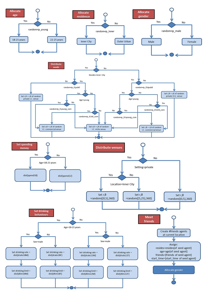
Setting up a simulation
- 2.8
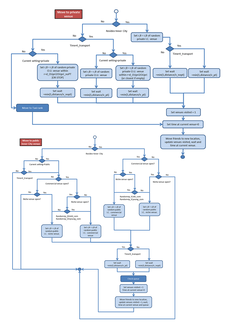
- The model is initially populated according to the six steps below. Parameters can be found in Appendix A, and further details are represented schematically by the flow diagrams in Appendix B.
- 2.9
- Each simulation is set up by: 1) generating and
distributing
venues throughout the model and allocating them their fixed properties;
2) generating a seed population of OU and IC residents and assigning
them each a friendship group size; 3) assigning the seed population to
start locations for their night; 4) creating additional agents
('friends') in the same location who are linked to the seed agents; 5)
allocating fixed properties (age, sex, drinking behaviours and spending
money) to all agents; and 6) making agents who do not commence their
drinking at \(t=0\) inactive at their current location (where they will
not interact with anything until their starting time). Each of these
steps is done according to the parameters in Appendix A.
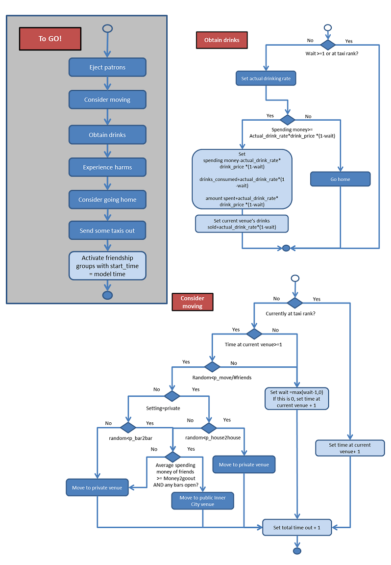
Agent behaviour
- 2.10
- Once the model is started seven main operations are
performed
each time step. Each of these steps is schematically represented in the
flow diagrams in Appendix B, and the corresponding parameters for each
decision are provided in Appendix A.
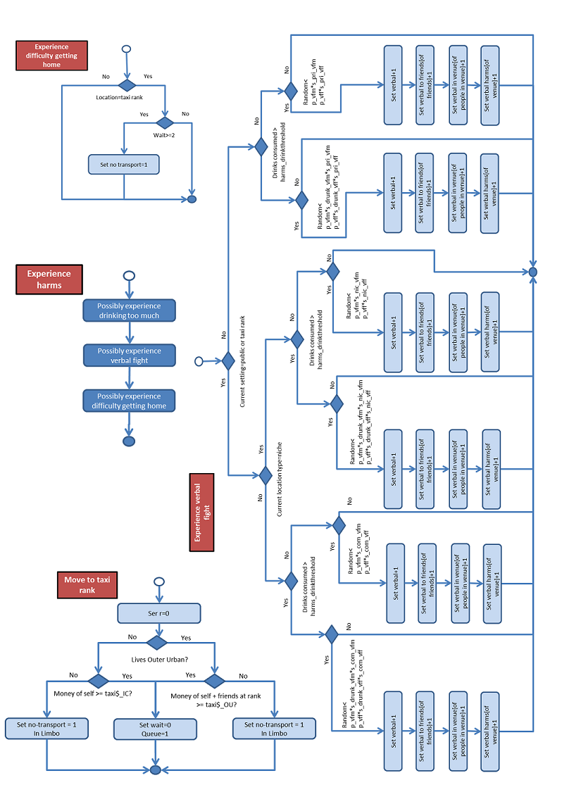
- Offer public venues a chance to eject
intoxicated patrons
or close
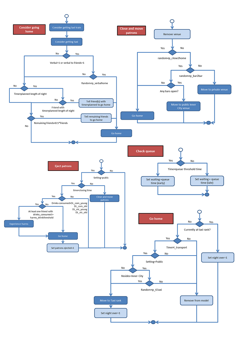
Public venues identify patrons who have consumed more than the venue's drink limit and force them to go home. If these agents have at least one friend who has consumed more than a harms threshold, they may experience harms as they leave (see step 4). If a public venue has reached closing time, all current patrons are offered a choice of whether to go home or move on to another venue—those choosing to move to another venue do so with their remaining friends. - Offer agents a chance to move between venues
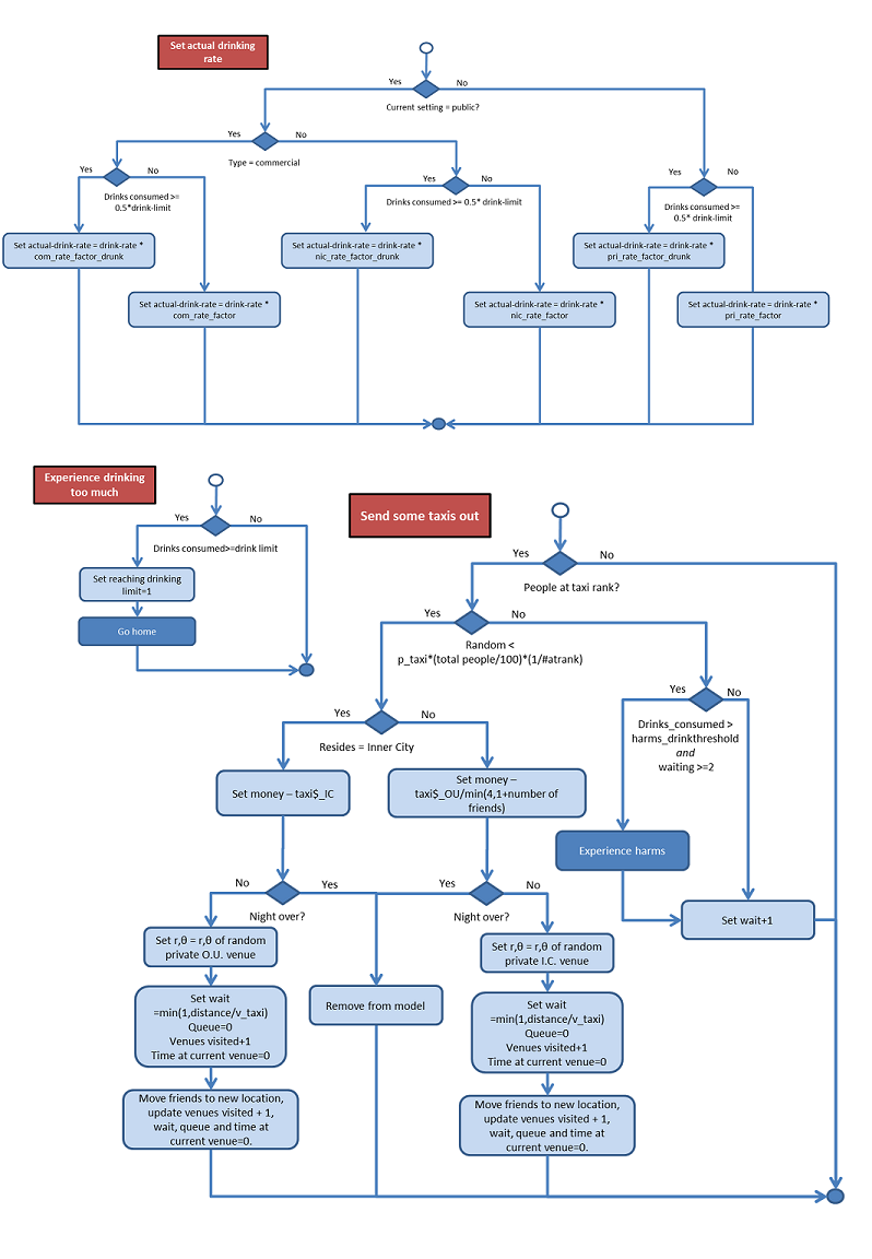
Agents who have been at a venue for an hour or more choose to either stay at the venue or move to another (Dietze et al. 2014; Miller et al. 2013). Those choosing to move take their entire friendship group with them (Miller et al. 2013), and their new location depends on their current setting type, their residence and the types of venues still open. The model assumes: agents only visit private locations near their residence (i.e. IC agents only go to private venues in the IC); agents don't move from OU private venues to the city once public transport has stopped; there is no gender differences in places visited; IC to IC travel is not done by taxi unless an IC resident is going home (when they choose whether to get a taxi or not); travel time between venues depends on mode of transport and is a maximum of one hour; and the cost of travel by public transport is negligible. - Offer agents a chance to consume drinks
Agents calculate their actual drinking rates: that is, they scale their fixed drinking rates depending on their current setting (private, public-niche, public-commercial) and whether they are intoxicated (agents decrease their drinking rate when they have consumed more than half their drinking limits). Agents then attempt to buy an hours' worth of drinks; however those who have just arrived at a venue must deduct travel and queueing time, and those who do not have enough money will buy only as many as they can afford. - Determine harms experienced by agents
Agents who have consumed more than their personal drinking limit are considered to have drunk too much and will go home. Agents can also experience verbal violence—this depends on their current location type and whether they have consumed more than a harms drink threshold (agents who have consumed more than 12 (men) or 6 (women) drinks are at increased risk of verbal violence—Appendix A). Agents are considered to have had difficulty getting home if they have spent two or more hours waiting for a taxi. - Get agents to consider going home
Agents are forced to go home if either: they have consumed more than their personal drink threshold; they are out of money; they and one or more of their friends have exceeded their planned length of night (Duff & Moore 2015); or if more than half of their initial friendship group has gone home. Agents may decide to go home if: they are in a public venue and the last train is about to leave (Duff & Moore 2015, this choice depends on their remaining money, the planned length of their night and where they live); they are in a public venue, public transport has stopped and they have only enough money for a taxi left; or if they or a friend have experienced some verbal violence. - Distribute some agents from the taxi rank to
their new
locations
Each time step agents waiting at the taxi rank have some chance of going to their new venue (either home or a private venue). This depends on the number of taxis (per 100 people) in the model and the current size of the queue. Agents who have been waiting for 2 or more hours for a taxi and have consumed more than a harms drinking threshold will loop through step 4 again. - Activate friendship groups
Friendship groups who have a start time corresponding to the current model time are activated and begin to interact with the rest of the model, 'starting' their night out.
- Offer public venues a chance to eject
intoxicated patrons
or close
Calibration
- 3.1
- A complete list of parameter values and their sources is provided in Appendix A. Public transport and venue setting properties have been determined using publicly available information for Melbourne (Public Transport Victoria 2015; Victorian Commission for Gambling and Liquor Regulation 2015), and where possible agent behaviour has been parametrized using the Young Adults Alcohol Study (YAAS, Dietze et al. 2014). Any remaining parameter estimates have been taken from available literature; where no studies were available to explicitly inform parameters, plausible estimates were made by the authors based on their extensive experience conducting social research on alcohol and other drug use in the night-time economy, including ethnographic research on young people's drinking events in OU and IC areas of Melbourne. These parameters were tested in a sensitivity analysis and as part of a Latin Hypercube uncertainty analysis.
- 3.2
- YAAS is a study of 802 young (18–25 year olds) people from Melbourne that asks specific questions about the most recent occasion when they consumed more than 7 (women) or 10 (men) standard drinks (in Australia, 10g of alcohol). This includes the number and types of venues attended; number of drinks consumed; total time and money spent in each venue; and whether or not verbal violence was experienced during the course of the night. Due to oversampling from particular areas, participants could be classified as residing in either the Local Government Areas (Department of Transport 2015) of Yarra (\(n=127\), proxy for IC), Hume (\(n=275\), proxy for OU) or the Rest of Melbourne (\(n=400\)). YAAS participants from Yarra or Hume have been used to determine model parameters, while participants from the Rest of Melbourne have had their nights compared to the outputs of the model to determine its accuracy. This procedure avoids using the dataset for both parameter determination and model calibration.
- 3.3
- Due to low reports of verbal violence among Yarra and Hume participants in the YAAS (\(N=28\) reported verbal violence on their most recent big night out), all YAAS data were used to determine the verbal violence harm parameters. Hence it is no longer valid to compare model outputs for these harms to those reported by YAAS participants from the Rest of Melbourne. However, a follow-up wave has since been conducted (\(N=531\) (66%) of the original sample were retained), and model outputs for verbal harms have been compared against those reported in the follow-up data.
- 3.4
- Among YAAS participants, verbal violence was more likely to
be
reported by older males, and on nights when more venues were visited,
more drinks were consumed, more hours were spent out and more money was
spent (Table 1). However, the
low number of
reports of verbal violence means that these differences were not
statistically significant and adjusted odds ratios provided no further
insight.
Table 1: Gender and age categories of individuals from the Young Adults Alcohol Study (Dietze et al. 2014) who experienced verbal violence on their most recent occasion consuming more than 7 (women)/10 (men) standard drinks; and characteristics of their nights. 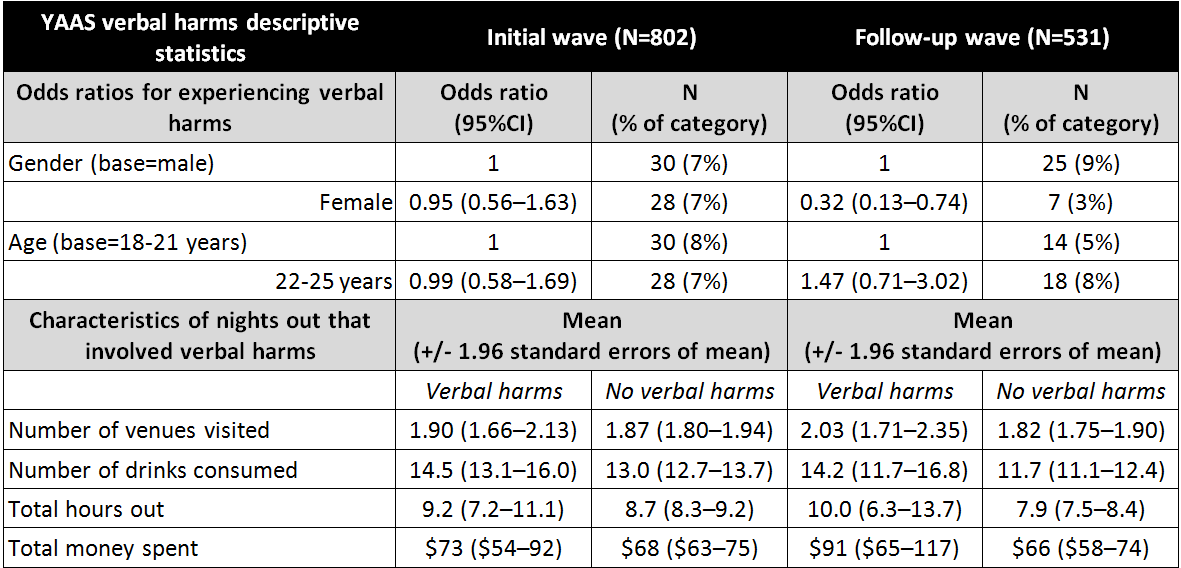
- 3.5
- Once parameters were determined (see Appendix A for further details), the model was run 100 times to account for stochastic variation and the output distribution properties (e.g. mean, median, interquartile range) of the results were compared to available data.
Model
robustness
- 4.1
- Many of the parameters in the model relate to the
likelihood of
individuals making particular decisions under specific circumstances;
for example p_PTrush_OU_plan_$ (Appendix A)—the probability that an
individual will choose to catch the last train home if they have less
than $50 left, had only planned to stay out for up to one hour longer
and live in an OU area. These types of features have been included
based on qualitative studies suggesting that they play a role in young
people's drinking events, with quantitative data either unavailable or
unfeasible to obtain for many of the related parameters. Nevertheless,
by including such features—even using authors' estimates for their
values—we believe the model has been improved, in particular as the
model outputs can now be probed for sensitivities when they vary.
Individual parameter variations
- 4.2
- To test model robustness to these unreferenced parameters, each was independently set to a lower bound and upper bound and 100 further simulations were undertaken.
- 4.3
- The differences in model outputs were measured when
parameters
were individually changed to test: a total of 50 friendship groups or
1000 friendship groups; a population of all women or all men; a
population of all 18–21 year olds or all 22–25 year olds; a population
of all IC residents or all OU residents; a total of 10 public venues or
500 public venues; all public venues niche or all public venues
commercial; individuals' planned length of nights distributed as
Poisson(6) or Poisson(10); individuals' drinking limits distributed as
Poisson(15/10) for men/women respectively or Poisson(25/20) for
men/women respectively; individuals never moving (unless the venue they
were in closed) or individuals moving each hour; no rush for the last
train or everyone rushing for the last train; no relative risk
differences for fights when drunk or in niche, private or commercial
venues or relative risks of 10 when drunk and 1:5:10 for
niche:private:commercial venues; no queues or queues of 0.75 hours and
0.33 hours for commercial and niche venues, respectively, all night; no
drink limits for public venues to eject patrons or public venues
ejecting patrons who had consumed greater than 15 (men)/10 (women)
standard drinks; no harms drink threshold or a threshold of 8 (men)/4
(women); no one going home after a verbal fight involving a member of
their friendship group or everyone going home; no one going home after
being in a venue that closed or everyone going home; and less expensive
taxis home ($10/$25 for IC/OU residents) and no required minimum money
to go to a public venue or more expensive taxis ($40/$80 for IC/OU
residents) and $50 minimum required to go to a public venue.
Uncertainty analysis using Latin Hypercube Sampling
- 4.4
- In addition to understanding how individual parameter changes affect model outputs, Latin Hypercube Sampling (Helton & Davis 2003; Iman 2008; Marino et al. 2008) was used to test the effects of jointly varying the above parameters. Continuous parameters were considered to be uniformly distributed between their lower and upper bounds, with 11 sample points (10 intervals) for each parameter. To attempt to separate variation due to parameter changes from the stochastic variation of the model, 10 simulations were run for each hypercube parameter sample and the average outputs were used as representatives of each point. The distribution of average outputs from these 11^(number of parameters) hypercube sample points were compared to the baseline point estimate distribution with stochastic variation.
- 4.5
- The large number of parameters made it unfeasible to perform this experiment on all variables at once, and so parameters were tested in five groups: 1) demographic parameters (gender, age, residence and number of friendship groups); 2) harm-related parameters (drinking limits, likelihood of going home after a fight, the harms drink threshold and scaling factors for verbal fights in different venue types and when drunk); 3) movement related parameters (planned length of nights, likelihood of moving each hour, likelihood of going home after a venue closes and likelihood of rushing for the last train); 4) venue characteristics (number of venues, type of venues, queue times, drink limits); and 5) costs (taxi price, money required to go out).
Results
-
Drinks consumed, amount spent and time spent drinking
- 5.1
- Although the model produces realistic distributions for the
total
drinks consumed, amount spent and time individuals spent out on a big
night, there are several disparities between the model outputs and
reports from YAAS participants from the Rest of Melbourne (Figure 1). First, the distribution of drinks
consumed by
YAAS participants is truncated below 8, whereas the model is not. This
is due to selection bias in YAAS; participants were only recruited into
the study if they reported recently consuming more than 7 (women) or
more than 10 (men) drinks in a single session. Second, total amount
spent in the model was left shifted (less money spent) than the
data—again most likely owing to selection bias in YAAS—and the modelled
amounts spent were more evenly distributed than the YAAS. This may in
part be due to survey participants rounding their total spending or
starting their night out with more discrete amounts of money: when $50
bins were used to plot spending greater than $100 in the model, the fit
was slightly improved. Third, the very highly skewed length of the
drinking session from YAAS was not reproduced by the model, largely
owing to the less skewed Gamma and Poisson distributions used to set up
agents' planned lengths of night, drinking limits, drinking rates and
spending money. Nevertheless, the initial peak of around 6–7 hours
spent drinking was captured by the model.
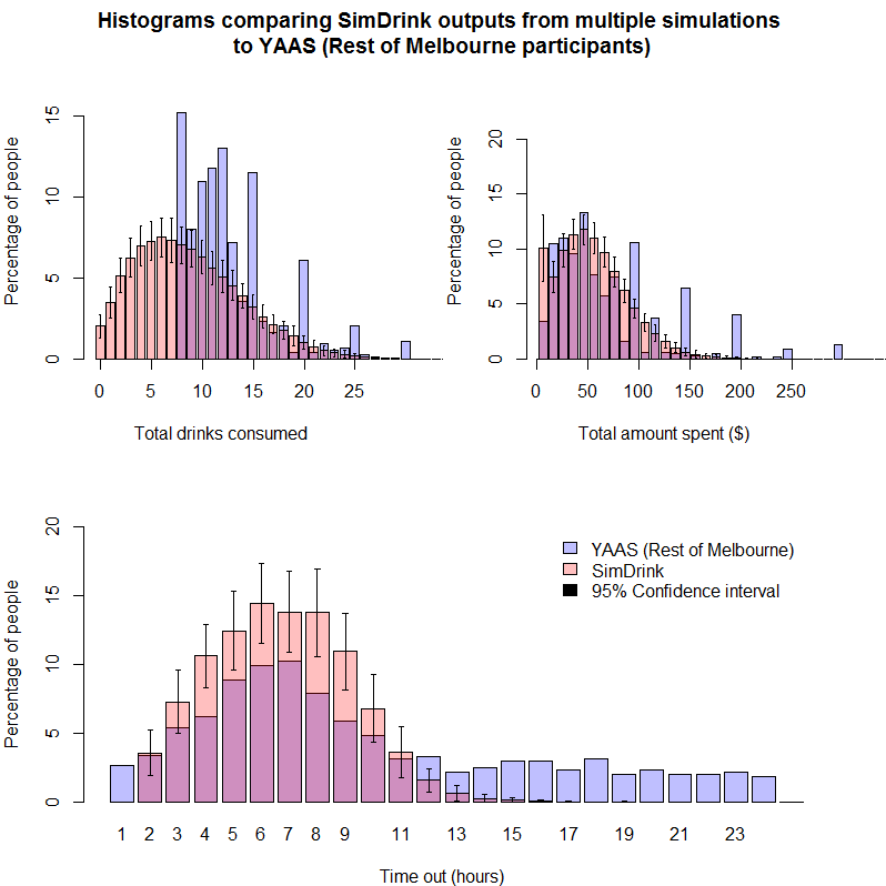
Figure 1. SimDrink outputs compared to the Young Adults Alcohol Study (YAAS). Comparison of total drinks consumed (top left), total amount spent (top right) and total time out (bottom) between the model and the survey results for young people enrolled in YAAS (excluding Hume and Yarra residents who were used to parametrise the model) describing their most recent 'big night out'. Model results include 95% confidence intervals from 100 simulations. Harms experienced
- 5.2
- The percentage of the modelled population who experienced each type of harm in the 100 simulations was measured. The median, interquartile range (IQR) and extremes are shown in the boxplots of Figure 2, compared to available data. Over these simulations, on a single night out a median of 6.33% (IQR 5.58–7.28%) of people experienced verbal violence; 13.63% (IQR 12.88–14.20%) of people drank more than their consumption limit; 25.16% (IQR 23.01–27.58%) witnessed verbal violence among their friendship group; and 5.42% (IQR 4.73–6.59%) of people had difficulty getting home.
- 5.3
- The only available data we found to compare this to (that
was not
used to determine model parameters) was the percentage of participants
in the YAAS follow-up wave who experienced verbal harms on their most
recent night out (6.18%), which was replicated well by the model.
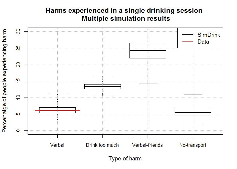
Figure 2. Harms in SimDrink. Median, interquartile range and upper / lower bounds for the percentage of people in the model who experienced verbal violence, drinking too much, a verbal fight involving a member of their friendship group and difficulty getting home. Results from 100 simulations. Sensitivity of parameters
- 5.4
- For each parameter variation, the prevalence of verbal
violence,
drinking too much and having trouble getting home on a given night out
are compared to best estimates in Figure 3.
Variations in outputs are logically valid and most are small, with the
greatest changes being in response to:
- Population size: a larger number of friendship groups resulted in a higher prevalence of verbal harms and an increase in the variability of the percentage who experienced consumption-related harms or difficulty getting home;
- Gender: an all-male population resulted in more people experiencing verbal harms (consistent with Table 1) and fewer people experiencing consumption-related harms;
- Planned length of night: an increase in the average planned length of night resulted in more people experiencing verbal harms (consistent with Table 1), consumption-related harms and having difficulty getting home;
- Drinking limits: higher drinking limits resulted in a higher prevalence of verbal harms and difficulty getting home and fewer people experiencing consumption-related harms;
- Frequency of moving between venues: a higher movement frequency resulted in more people experiencing consumption-related harms but fewer people experiencing verbal harms and difficulty getting home (note that this does not directly compare to Table 1, since movement frequency combines with planned length of night to influence number of venues visited—see the Latin Hypercube uncertainty analysis);
- Last train: a certainty of rushing for the last train resulted in a lower prevalence of verbal harms and fewer people experiencing difficulty getting home (note that people from the IC can still move from a private venue to a public venue after public transport has finished, and so can still experience difficulty getting home); and
- Responsible service of alcohol (RSA): ejecting intoxicated people from public venues sooner resulted in a higher prevalence of verbal harms and fewer people experiencing consumption-related harms or difficulty getting home.
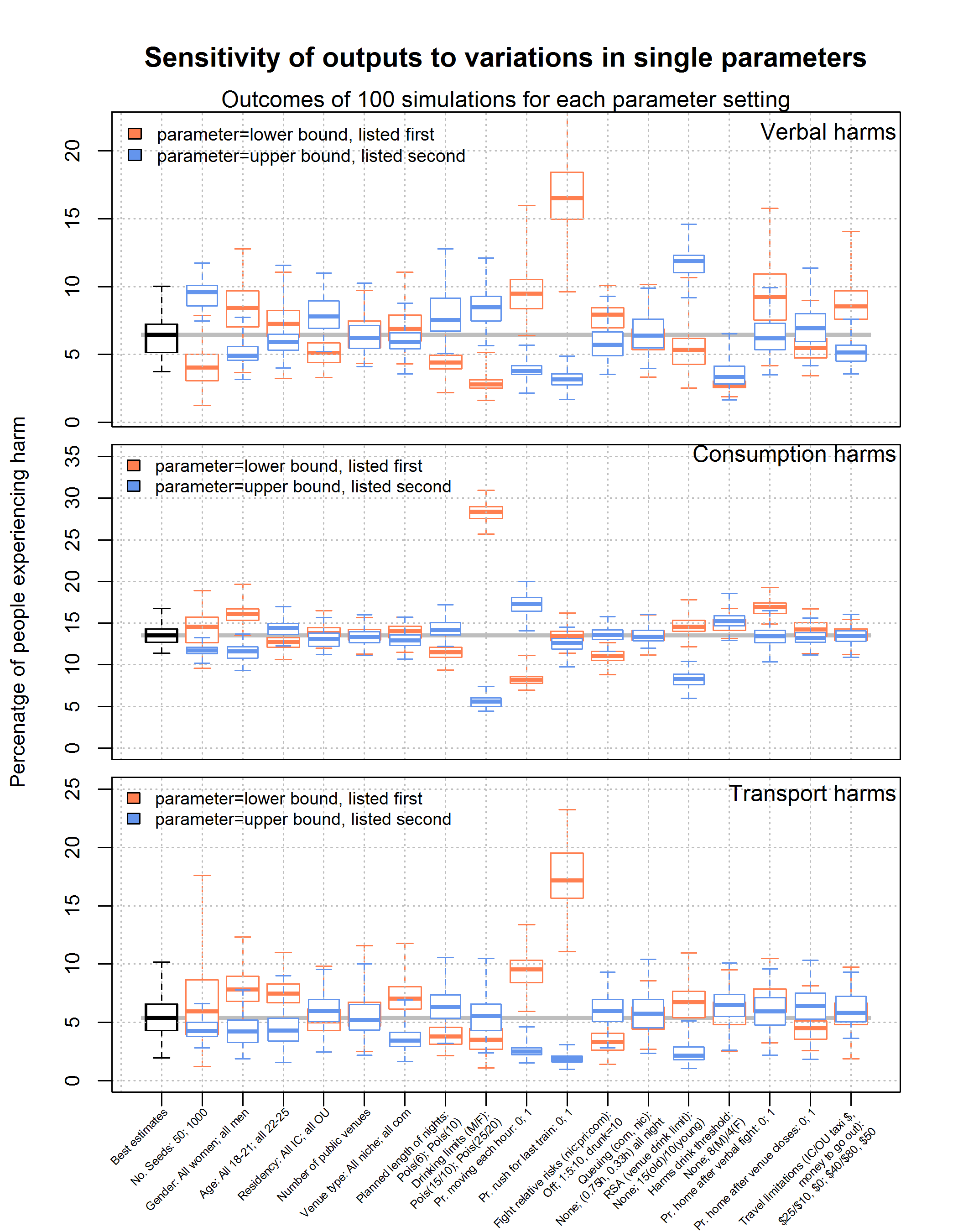
Figure 3. Sensitivity of harms. The effects on verbal, consumption-related and transport-related harms of changes in: population size; gender; age; residency; number of venues; venue types; planned length of night and drinking limit distributions; the likelihood of moving each hour; relative risks of fights when drunk or in niche (nic), private (pri) and commercial (com) venues; queueing times; responsible service of alcohol (RSA) enforcement; the harms drink threshold; the likelihood of going home after a verbal fight; the likelihood of going home after a venue closes; and travel limitations. Box plots represent median, inter-quartile range and lower/upper bounds from 100 simulation outputs. Latin Hypercube uncertainty analysis
- 5.5
- Relative to the stochastic variation of the model,
demographic,
harm-related and movement parameters played a significant role in the
prevalence of all three types of harm, while the venue and cost
parameters had little influence on model outcomes (Figure 4). In particular, there were some
samples of the
harm-related parameters that resulted in more than 30% of the
population experiencing verbal harms. This indicates that these
parameters are important to the model and assumptions about their
values should be detailed when using the model to make predictions.
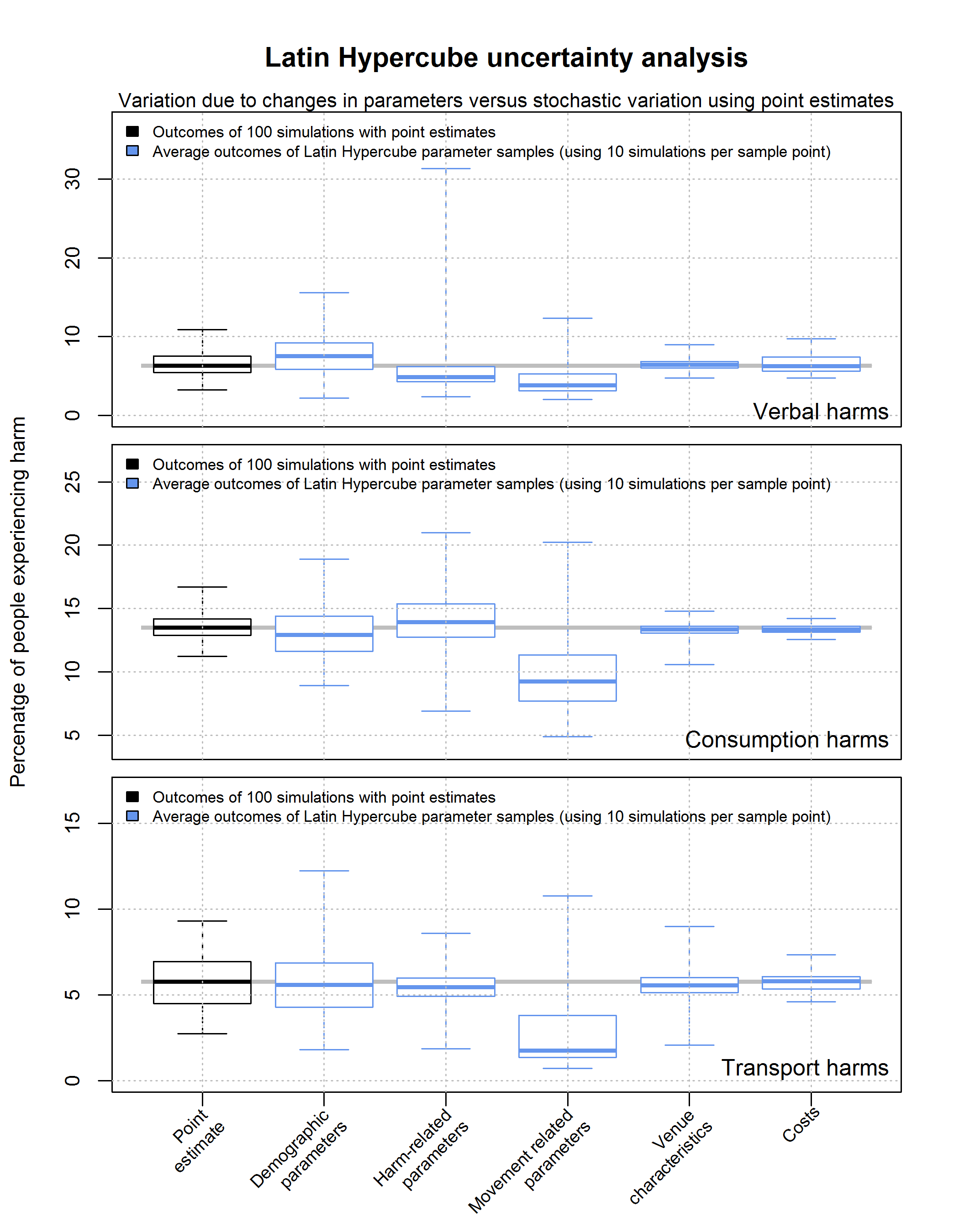
Figure 4. Latin Hypercube uncertainty analysis. Blue boxplots: Variation in the average (after 10 simulations) percentage of people experiencing harms when parameters are taken from every point on the Latin Hypercube, for demographic parameters (gender, age, residence and number of friendship groups), harm-related parameters (drinking limits, likelihood of going home after a fight, the harms drink threshold and scaling factors for verbal fights in different venue types and when drunk), movement related parameters (planned length of nights, likelihood of moving each hour, likelihood of going home after a venue closes and likelihood of rushing for the last train), venue characteristics (number of venues, type of venues, queue times, drink limits), and costs (taxi price, money required to go out). Black boxplot: stochastic variation from 100 simulations with point estimate parameters.
Limitations
- 6.1
- The model has several limitations owing to either its complexity or the lack of available data. First, limited studies are available that could be used to estimate many of the parameters, and the current calibration relies heavily on the YAAS data. In particular, using participants from Yarra and Hume to calibrate IC and OU populations respectively while keeping those living everywhere else for validation may have introduced some bias, and parameters should be updated as independent studies become available. Nevertheless, the model remains a useful proof-of-concept tool, and we emphasize that it should be used to compare multiple policy options rather than to directly estimate the effects of individual policies. This is especially the case for situations where particular sub-groups are of interest, since the model is only calibrated to overall outcomes and the uncertainty analysis suggests that differences in the simulated population may be important. Second, even though the model allows large amounts of heterogeneity, some properties are categorised, such as the age (categorised as 18–21 year olds and 22–25 year olds) and residence (categorised as OU or IC) of individuals. It is unclear how, for example, the propensity of individuals to rush to get the last train varies with distance from the CBD, or how drinking limits and rates vary continuously as age increases. However given the lack of data to investigate these relationships, categorising such variables seems appropriate. Third, agent characteristics have been drawn independently from probability distributions while in practice these characteristics would exhibit some degree of correlation among social groups. Should appropriate individual-level data become available, adjustments are possible that would enable the model to use joint probability distributions to configure agent properties.
Further
work
-
Applications and model extensions
- 7.1
- Further work with policy makers is required to identify specific harm reduction interventions that can be virtually implemented and compared. For example, Melbourne City Council's Transport Strategy (City of Melbourne 2012) involves improving the late night accessibility of the CBD, one proposal being to extend public transport operating hours. The effects of such a policy change could be tested in this model and compared to alternate scenarios (for example improvements to taxi availability). Other policies that aim more explicitly to reduce alcohol related harms that could be tested include: venue lockouts—where individuals are allowed to remain in venues but no longer enter after a particular time (Department of Justice 2008; Menéndez et al. 2015); increasing the taxation of alcohol (both on and off licence) (Skov 2009); changing venue operations by restricting opening hours (Cobiac et al. 2009); and training bar staff to more strictly enforce responsible service of alcohol (Graham et al. 2004; Lang et al. 1998). Each of these policies is likely to affect different groups in different ways (for example OU and IC residents, niche or commercial venues), and changes to the prevalence of verbal, consumption and transport-related harms—both direct and indirect—are captured in the model. This will allow evidence based decisions to be made on the most effective interventions, ensuring they have their intended effects.
- 7.2
- The high versatility of ABMs means that the model can
easily be
expanded as further data becomes available or in order to address
specific policy questions. For example, physical violence in the
night-time economy is a concern for police and policy makers, and if
data became available on the prevalence of experiencing physical
violence on a single night out, this feature could be included.
Methodological improvements could also be made. For example, by using
global positioning system co-ordinates for venue locations and
including more detailed neighbourhoods (with populations parametrised
by census data), the model could be used for a geo-simulation. In such
a scenario the accessibility of public transport could also be varied
across neighbourhoods. Finally, as more studies are undertaken to
understand the consumption event, different theoretical models could be
developed and tested regarding the distributions that have been assumed
for parameters such as the planned lengths of nights, drinking limits
and drinking rates, with outputs fit to observed data accordingly.
Areas identified for future alcohol studies
- 7.3
- The construction of this model has identified many areas in alcohol research that are lacking any empirical data. Most importantly and perhaps surprisingly, no data could be identified on the prevalence of consumption-related and transport-related harms on an individual night out. Other parameters and distributions that were important for this model, but could not be informed by sufficient data (limited or no studies available), included individual drinking limits, planned lengths of nights, the frequency of movements between venues and the probability of individuals rushing to get the last train. Beyond their significance for this model, these parameters would be extremely useful for alcohol research more broadly, in particular in the context of understanding the consumption event.
Conclusion
- 8.1
- We have constructed a proof-of-concept ABM to simulate a population of 18-25 year olds engaging in heavy sessional drinking on a night out in Melbourne. The model includes demographic, setting and situational-behavioural heterogeneity and produces realistic estimates for the prevalence of various types of acute alcohol related harm. As parameters vary across their domains changes in outputs are logically valid and modest, indicating that the model is robust and internally consistent. Further, the model is able to compare the indirect effects of policy changes such as the displacement of individuals or venue substitution, making it a particularly attractive for modelling policy decisions and identifying the drivers behind overall statistics.
Acknowledgements
- The research reported here was funded by an Australian Research Council Discovery Project (DP110101720). The authors gratefully acknowledge the contribution to this work of the Victorian Operational Infrastructure Support Program. The National Drug Research Institute is supported by funding from the Australian Government under the Substance Misuse Prevention and Service Improvement Grants Fund. NS is the recipient of a Burnet Institute Jim and Margaret Beever Fellowship, PD is the recipient of a National Health and Medical Research Council (NHMRC) Senior Research Fellowship and ML is the recipient of an NHMRC Early Career Fellowship.
Appendix
A
-
Table A1: Model parameters and references Variable Description Value Source Comments Setup
N_seeds Number of seeds to start the model. 300 Sensitivity analysis Combine with friend distribution for total population size. p_male Proportion of men. 0.5 Sensitivity analysis
p_young Proportion of 18-21 year olds (versus 21-25 year olds). 0.5 Sensitivity analysis
p_inner Proportion from the Inner City. 0.5 Sensitivity analysis
N_public Number of public (Inner City) venues. 100 Sensitivity analysis
N_privateOU Number of private Outer Urban venues. 500 Sensitivity analysis No impact, not shown. N_privateIC Number of private Inner City venues. 500
p_ICpub0 Proportion of Inner City residents starting in public venue. 0.31 YAAS (Dietze et al. 2014) Proportion of Yarra residents starting in public venues. p_OUpub0 Proportion of Outer Urban residents starting in public venue. 0.27 YAAS (Dietze et al. 2014) Proportion of Hume residents starting in public venues. Agent properties
dist(friend) Distribution of number of friends. Poisson(5.69) POINTED (Miller et al. 2013) Fit to survey results. dist(length) Distribution of the planned length of nights. Poisson(8) YAAS (Dietze et al. 2014) Poisson curve fitted to Hume and Yarra residents' total time out. dist(start) Distribution of starting times for night out. Gamma(78.313,4.094) YAAS (Dietze et al. 2014) Fit to the time of first drink for Hume and Yarra residents, truncated to be between 5pm and 11pm. dist(dlim18M) Distribution of 18-21 year old drinking limits, men. Poisson(20) Sensitivity analysis Authors' estimate.
Consumption limits for young and old assumed to be the same (however they behave differently).dist(dlim22M) Distribution of 22-25 year old drinking limits, men. Poisson(20)
dist(dlim18F) Distribution of 18-21 year old drinking limits, women. Poisson(15)
dist(dlim22F) Distribution of 22-25 year old drinking limits, women. Poisson(15)
dist(spend18) Distribution of 18-21 year old spending money. Gamma(3.456,0.026) YAAS (Dietze et al. 2014) Fit to total spent on night out, by 18-21 year old participants from Hume and Yarra who spent >=$50.
Similarly for 22-25 year olds.dist(spend22) Distribution of 22-25 year old spending money. Gamma(3.279,0.024)
dist(drate18M) Distribution of 18-21 year old drinking rates, men. Gamma(2.634,1.006) YAAS (Dietze et al. 2014) For male 18-21 year old Hume and Yarra residents who attended a private venue first. Fit to distribution of:
Total drinks/time in in first venue.
Similarly for other age/sex categories.dist(drate22M) Distribution of 22-25 year old drinking rates, men. Gamma(2.643,1.238)
dist(drate18F) Distribution of 18-21 year old drinking rates, women. Gamma(1.744,0.970)
dist(drate22F) Distribution of 22-25 year old drinking rates, women. Gamma(4.451,2.707)
s_pri_rate Drink rate scaling factor in private venues. 1 YAAS (Dietze et al. 2014) Definition. s_com_rate Drink rate scaling factor in commercial venues. 1.46 YAAS (Dietze et al. 2014) For Hume and Yarra residents, at first venue attended, determine: mean drinking rate of (18-21 year old male) participants in commercial venues / mean drinking rate of (18-21 year old male) participants in private venues.
Average across age and sex categories.
Similarly for niche venues.s_nic_rate Drink rate scaling factor in niche venues. 1.00
s_pri_rate_drunk Drink rate scaling factor in private venues after drinking more than half personal drink limit. 0.76 YAAS (Dietze et al. 2014) Average for Hume and Yarra residents of: drinking rate in last venue of evening (for people ending in a private venue, having attended two or more venues) / average drink rate in first venue (if it was private).
Similarly for nightclubs and pub/bar venues.s_com_rate_drunk Drink rate scaling factor in commercial venues after drinking more than half personal drink limit. 0.63
s_nic_rate_drunk Drink rate scaling factor in niche venues after drinking more than half personal drink limit. 0.89
Setting properties
dist(CT_com) Distribution of commercial venue closing times. (2am, 3am, 4am, 5am, 6am, 7am)=
(6, 167, 7, 32, 1, 77)/290(Victorian Commission for Gambling and Liquor Regulation 2015) Melbourne liquor licensing reports.
Commercial venues considered to be venues with "Late night (general) Licence"; Niche bars considered to be venues with "General Licence – Trading to 12am/1am", "On-Premises Licence – Trading to 12am/1am" or "Late night (on-premises) Licence".dist(CT_nic) Distribution of niche venue closing times. (12am, 1am, 2am, 3am, 4am, 5am,6am,7am)=
(120, 862, 16, 197, 13, 38, 2, 35)/1283(Victorian Commission for Gambling and Liquor Regulation 2015)
p_commercial Proportion of public venues that are commercial (vs niche). 0.18
dist(QT_com) Distribution of commercial venue queueing times (early). 0 Sensitivity analysis Authors' estimate. No queues for niche venues that close before 1am. dist(QT_com_late) Distribution of commercial venue queueing times (late). 0.5 hour
dist(QT_nic) Distribution of niche venue queueing times (early). 0 hour
dist(QT_nic_late) Distribution of niche venue queueing times (late). 0.333 hour
queue_time Time of night that queues become longer. 10pm Sensitivity analysis Based on cover charges, drink deals. dist(DL_com_young) Distribution of commercial venue drink limits (18-21). 18 Sensitivity analysis Authors' estimate.
Older people are thought to be more in control when intoxicated (Demant & Järvinen 2010).dist(DL_com_old) Distribution of commercial venue drink limits (22-25). 20
dist(DL_nic_young) Distribution of niche venue drink limits (18-21). 18
dist(DL_nic_old) Distribution of niche venue drink limits (22-25). 20
p_freedrink Proportion of private venues where drinks are free. 0.15 YAAS (Dietze et al. 2014) Proportion of private venues visited by Hume and Yarra residents where drinks were consumed and no money was spent (including money spent on them by others). $_com Drink price in commercial venues. $9.72 YAAS (Dietze et al. 2014) Total amount spent by Hume and Yarra residents on drinks in commercial venues (including what others spent on them)/total drinks they consumed there. Only includes venues where spending >0.
Similarly for niche and private venues.$_nic Drink price in niche venues. $8.56
$_pri Drink price in private venues. $5.08
Movements
money2goout Average spending money of friends required for group to go to public venue. $30 Sensitivity analysis Authors' estimate. p_taxi Probability of getting a taxi (per hour): number of taxis per 100 people in the model, assuming they are all available for one trip per hour. I.e. pr(getting taxi each hour)=(#people/100) * p_taxi * (1/taxiqueue). 1/100 people Calibration Parameter can be used to calibrate the percentage of people experiencing transport harms. Increases / decreases the number of taxis in the model. v_pt Public transport travel speed. 25km/h Sensitivity analysis Used to define movement times in model. v_nopt Travel speed with no public transport. 10km/h
v_taxi Taxi speed. 60 km/h
taxi$_OU Cost of a taxi to Outer Urban private / home. $50
taxi$_IC Cost of a taxi to Inner City private / home. $25
d_OUpri2OUpri Agents travelling Outer Urban private-Outer Urban private will preference venues in this radius when public transport is available. 15km
d_OUpri2OUpri_noPT Agents travelling Outer Urban private-Outer Urban private will preference venues in this radius when public transport is not available. 5km
p_move Probability of a group of friends moving each hour. 0.12 YAAS (Dietze et al. 2014) Total venue changes / total time out of Hume and Yarra residents. p_ICyoung_com Probability that a public venue visited by an 18-21 year old Inner City resident is commercial. 0.38 YAAS (Dietze et al. 2014) Number of commercial venues visited by 18-21 year old Yarra residents / number public venues visited by 18-21 year old Yarra residents.
Similarly for 22-25 year olds and Hume residents.P_ICold_com Probability that a public venue visited by a 22-25 year old Inner City resident is commercial. 0.34
p_OUyoung_com Probability that a public venue visited by an 18-21 year old Outer Urban resident is commercial. 0.47
p_OUold_com Probability that a public venue visited by a 22-25 year old Outer Urban resident is commercial. 0.38
p_bar2bar Probability of moving public to public (vs public to private). 0.78 YAAS (Dietze et al. 2014) Total public-public movements of Hume and Yarra residents/total public-public + public-private movements. p_house2house Probability of moving private to private (vs private to public). 0.26 YAAS (Dietze et al. 2014) Total private-private movements of Hume and Yarra residents/total private-private + private-public movements. t_transport Time when public transport turns off. 1am Public Transport Victoria (Public Transport Victoria 2015) Last outbound train from the city. p_PTrush_OU_plan_$ Pr of rushing for last train, Outer Urban resident, within hour of planned length, not enough left for taxi. 0.6 Sensitivity analysis Authors' estimate. p_PTrush_OU_plan Pr of rushing for last train, Outer Urban resident, within hour of planned length. 0.4
p_PTrush_OU_$ Pr of rushing for last train, Outer Urban resident, not enough left for taxi. 0.2
p_PTrush_OU Pr of rushing for last train, Outer Urban resident. 0.1
p_PTrush_IC_plan_$ Pr of rushing for last train, Inner City resident, within hour of planned length, not enough left for taxi. 0.4
p_PTrushIC_plan Pr of rushing for last train, Inner City resident, within hour of planned length. 0.2
p_PTrush_IC_$ Pr of rushing for last train, Inner City resident, not enough left for taxi. 0.1
p_PTrush_IC Pr of rushing for last train, Inner City resident. 0
p_ICtaxi Probability of an Inner City resident trying to get a taxi home after public transport stops (compared to walking). 0.5
p_lastchancetaxi_OU Probability Outer Urban resident using the last of their money to get home. 0.5
p_lastchancetaxi_IC Probability Inner City resident using the last of their money to get home. 0.2
p_close2home Probability of going home after a venue closes. 0.5 Sensitivity analysis Authors' estimate. Harms
harms_drinkthreshold Above this many drinks consumed people are at greater risks of verbal fights. 12 (M) / 6 (F) Sensitivity analysis Authors' estimate. s_pri_vfm Verbal fight, scaling factor for private venue (relative to niche venue), men. 2.5 Sensitivity analysis Authors' estimate. s_com_vfm Verbal fight, scaling factor for commercial venue (relative to niche venue), men. 5
s_drunk_vfm Verbal fight, scaling factor when consumed more than harms_drinkthreshold drinks, men. 5
p_vfm Verbal fight per person-hour, niche venue, men. 0.00127 YAAS (Dietze et al. 2014) Dependent on scaling factors and harms_drinkthreshold. Let time_nic_m and time_nic_m_drunk be the total person hours in YAAS spent by men in niche venues before and after harms_drinkthreshold drinks were consumed respectively. For venues where the drink threshold is crossed, all time is counted towards time_nic_m_drunk.
Then
p_vfm = total verbal fights for men / [
time_nic_m + time_pri_m*s_pri_vfm + time_com_m*s_com_vfm + s_drunk_vfm*(time_nic_m_drunk + time_pri_m_drunk*s_pri_vfm + time_com_m_drunk*s_com_vfm)].
Uses participants from all LGAs.s_pri_vff Verbal fight, scaling factor for private venue (relative to niche venue), women. 2.5 Sensitivity analysis Authors' estimate. s_com_vff Verbal fight, scaling factor for commercial venue (relative to niche venue), women. 5
s_drunk_vff Verbal fight, scaling factor when consumed more than harms_drinkthreshold drinks, women. 5
p_vff Verbal fight per person-hour, niche venue, women. 0.00088 YAAS (Dietze et al. 2014) Analogous to p_vfm. Uses participants from all LGAs. p_verbalhome Probability of going home after a friend has a verbal argument. 0.7 Sensitivity analysis Authors' estimate.
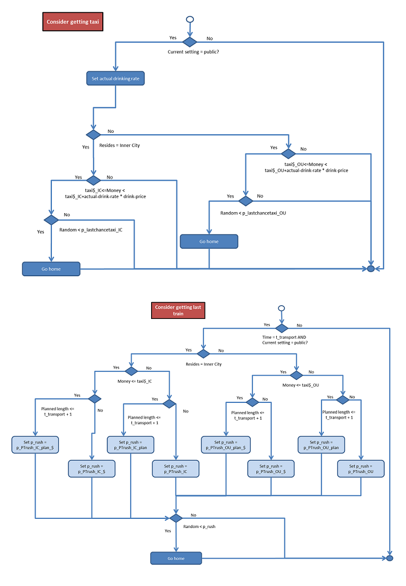
Appendix
B: Flow diagrams describing the model
References
- AUSTRALIAN
INSTITUTE OF HEALTH AND WELFARE. (2013). National Drug
Strategy
Household Survey 2013 - Detailed Report. Canberra, AIHW.
BØHLING, F. (2014). Crowded contexts: On the affective dynamics of alcohol and other drug use in nightlife spaces. Contemporary Drug Problems, 41(3), 361. [doi:10.1177/009145091404100305]
CALLINAN, S., Livingston, M., Dietze, P., & Room, R. (2014). Heavy drinking occasions in Australia: Do context and beverage choice differ from low-risk drinking occasions? Drug and alcohol review, 33(4), 354–357. [doi:10.1111/dar.12135]
CALLINAN, S., Room, R., Livingston, M., & Jiang, H. (2015). Who purchases low cost alcohol in Australia? Alcohol and Alcoholism, agv066. [doi:10.1093/alcalc/agv066]
CASTIGLIONE, F., Pappalardo, F., Bernaschi, M., & Motta, S. (2007). Optimization of HAART with genetic algorithms and agent-based models of HIV infection. Bioinformatics, 23(24), 3350–3355. [doi:10.1093/bioinformatics/btm408]
CECCHINI, M., M. Devaux, & Sassi, F. (2015) Assessing the impacts of alcohol policies. OECD Health Working Papers.
CITY OF MELBOURNE. (2012). Transport Strategy 2012: Planning for Future Growth. http://melbourne.vic.gov.au/futuregrowth.
COBIAC, L., Vos, T., Doran, C., & Wallace, A. (2009). Cost-effectiveness of interventions to prevent alcohol-related disease and injury in Australia. Addiction, 104(10), 1646–1655. [doi:10.1111/j.1360-0443.2009.02708.x]
DEMANT, J., & Järvinen, M. (2010). Social capital as norms and resources: Focus groups discussing alcohol. Addiction Research & Theory, 19(2), 91–101. [doi:10.3109/16066351003725776]
DEPARTMENT OF JUSTICE. (2008). Evaluation of the Temporary Late Night Entry Declaration, Final Report.
DEPARTMENT OF TRANSPORT, Planning and Local Infrastructure. (2015). http://www.dpcd.vic.gov.au/localgovernment/find-your-local-council#councils
DIETZE, P. M, Livingston, M., Callinan, S., & Room, R. (2014). The big night out: What happens on the most recent heavy drinking occasion among young Victorian risky drinkers? Drug and alcohol review, 33(4), 346–353. [doi:10.1111/dar.12117]
DILKES-FRAYNE, E. (2014). Tracing the 'event' of drug use: Examining 'context' and the co-production of a night out on MDMA. . Contemporary Drug Problems, 41(2). [doi:10.1177/009145091404100308]
DRAY, A., Mazerolle, L., Perez, P., & Ritter, A. (2008). Policing Australia's 'heroin drought': using an agent-based model to simulate alternative outcomes. Journal of Experimental Criminology, 4(3), 267–287. [doi:10.1007/s11292-008-9057-1]
DRAY, A., Perez, P., Moore, D., Dietze, P., Bammer, G., Jenkinson, R., Siokou, C., Hudson, S. & L. Maher, L. (2012). Are drug detection dogs and mass-media campaigns likely to be effective policy responses to psychostimulant use and related harm? Results from an agent-based simulation model. International Journal of Drug Policy, 23(2), 148–153. [doi:10.1016/j.drugpo.2011.05.018]
DUFF, C., & Moore, D.. (2015). Going out, getting about: atmospheres of mobility in Melbourne's night-time economy. Social & Cultural Geography, 16(3), 299–314. [doi:10.1080/14649365.2014.979864]
GALEA, S., Hall, C., & Kaplan, G. A. (2009). Social epidemiology and complex system dynamic modelling as applied to health behaviour and drug use research. International Journal of Drug Policy, 20(3), 209–216. [doi:10.1016/j.drugpo.2008.08.005]
GIABBANELLI, P., & Crutzen, R. (2013). An agent-based social network model of binge drinking among Dutch adults. Journal of Artificial Societies and Social Simulation, 16(2), 10. [doi:10.18564/jasss.2159]
GILBERT, N. (2008). Agent-based models. London: Sage.
GORMAN, D. M, Mezic, J., Mezic, I., & Gruenewald, P. J. (2006). Agent-based modeling of drinking behavior: a preliminary model and potential applications to theory and practice. American Journal of Public Health, 96(11), 2055–2060. [doi:10.2105/AJPH.2005.063289]
GRAHAM, K., Osgood, D W., Zibrowski, E., Purcell, J., Gliksman, L., Leonard, K., Pernanen, K., Saltz, R. F. & Toomey, T. L. (2004). The effect of the Safer Bars programme on physical aggression in bars: results of a randomized controlled trial. Drug and alcohol review, 23(1), 31–41. [doi:10.1080/09595230410001645538]
HART, A. (2015). Assembling Interrelations Between Low Socioeconomic Status and Acute Alcohol-Related Harms Among Young Adult Drinkers. Contemporary Drug Problems, 0091450915583828. [doi:10.1177/0091450915583828]
HELTON, J. C, & Davis, F, J. (2003). Latin hypercube sampling and the propagation of uncertainty in analyses of complex systems. Reliability Engineering & System Safety, 81(1), 23–69. [doi:10.1016/S0951-8320(03)00058-9]
IMAN, Ronald L. (2008). Latin Hypercube Sampling Encyclopedia of Quantitative Risk Analysis and Assessment: John Wiley & Sons, Ltd.
KRETZSCHMAR, M., & Wiessing, L. G. (1998). Modelling the spread of HIV in social networks of injecting drug users. Aids, 12(7), 801–811. [doi:10.1097/00002030-199807000-00017]
KUNTSCHE, E., Dietze, P., & Jenkinson, R. (2014). Understanding alcohol and other drug use during the event. Drug and Alcohol Review, 33(4), 335–337. [doi:10.1111/dar.12171]
KYPRI, K., Jones, C., McElduff, P., & Barker, D. (2011). Effects of restricting pub closing times on night-time assaults in an Australian city. Addiction, 106(2), 303–310. [doi:10.1111/j.1360-0443.2010.03125.x]
LANG, E., Stockwell, T. I. M., Rydon, P., & Beel, A. (1998). Can training bar staff in responsible serving practices reduce alcohol-related harm? Drug and Alcohol Review, 17(1), 39–50. [doi:10.1080/09595239800187581]
LINDSAY, J. (2005). Drinking in Melbourne pubs and clubs: A study of alcohol consumption contexts: School of Political and Social Inquiry, Monash University Clayton, Australia.
LIVINGSTON, M. (2008). A longitudinal analysis of alcohol outlet density and assault. Alcoholism: Clinical and Experimental Research, 32(6), 1074–1079. [doi:10.1111/j.1530-0277.2008.00669.x]
MACLEAN, S., & Callinan, S. (2013). "Fourteen Dollars for One Beer!" Pre-drinking is associated with high-risk drinking among Victorian young adults. Australian and New Zealand journal of public health, 37(6), 579–585. [doi:10.1111/1753-6405.12138]
MACLEAN, S., Ferris, J., & Livingston, M. (2013). Drinking patterns and attitudes for young people in inner-urban Melbourne and outer-urban growth areas: Differences and similarities. Urban Policy and Research, 31(4), 417–434. [doi:10.1080/08111146.2013.831758]
MACLEAN, S., & Moore, D. (2014). 'Hyped up': Assemblages of alcohol, excitement and violence for outer-suburban young adults in the inner-city at night. International Journal of Drug Policy, 25(3), 378–385. [doi:10.1016/j.drugpo.2014.02.006]
MARINO, S., Hogue, I. B, Ray, C. J, & Kirschner, D. E. (2008). A methodology for performing global uncertainty and sensitivity analysis in systems biology. Journal of theoretical biology, 254(1), 178–196. [doi:10.1016/j.jtbi.2008.04.011]
MEIER, P. S., Purshouse, R., & Brennan, A. (2010). Policy options for alcohol price regulation: the importance of modelling population heterogeneity. Addiction, 105(3), 383–393. [doi:10.1111/j.1360-0443.2009.02721.x]
MENÉNDEZ, P., Weatherburn, D., Kypri, K., & Fitzgerald, J. (2015). Lockouts and last drinks: The impact of the January 2014 liquor licence reforms on assaults in NSW, Australia. NSW Bureau of Crime Statistics and Research, Crime and Justice Bulletin.
MERCKEN, L., Steglich, C., Knibbe, R., & De Vries, H. (2015). Dynamics of friendship networks and alcohol use in early and mid-adolescence. Journal of Studies on Alcohol and Drugs.
MILLER, P., Chikritzhs, Y., & Toumbourou, J. (2015). Interventions for reducing alcohol supply, alcohol demand and alcohol-related harm. National Drug Law Enforcement Research Fund (NDLERF), Monograph no. 57.
MILLER, P., Pennay, A., Droste, N., Jenkinson, R., Quinn, B., & Chikritzhs, T. (2013). Patron offending and intoxication in night time entertainment districts (POINTED): final report. National Drug Law Enforcement Research Fund.
MOORE, D., Dray, A., Green, R., Hudson, S. L., Jenkinson, R., Siokou, C., Perez, P., Bammer, G., Maher, L., & Dietze, P. (2009). Extending drug ethno-epidemiology using agent-based modelling. Addiction, 104(12), 1991–1997. [doi:10.1111/j.1360-0443.2009.02709.x]
OECD. (2015). Tackling Harmful Alcohol Use: Economics and Public Health Policy. OECD Publishing.
ORMEROD, P., & Wiltshire, G. (2009). 'Binge'drinking in the UK: a social network phenomenon. Mind & Society, 8(2), 135–152. [doi:10.1007/s11299-009-0058-1]
PUBLIC TRANSPORT VICTORIA. (2015). http:http://ptv.vic.gov.au.
ROLLS, D. A., Wang, P., Jenkinson, R., Pattison, P. E., Robins, G. L., Sacks-Davis, R., Daraganova, G., Hellard, M. & McBryde, E. (2013). Modelling a disease-relevant contact network of people who inject drugs. Social Networks, 35(4), 699–710. [doi:10.1016/j.socnet.2013.06.003]
ROOM, R. (1988). The dialectic of drinking in Australian life: from the Rum Corps to the wine column. Drug and alcohol review, 7(4), 413–437. [doi:10.1080/09595238880000741]
SKOV, S. J. (2009). Alcohol taxation policy in Australia: public health imperatives for action. The Medical journal of Australia, 190(8), 437–439.
THIELE, J. (2014). R marries NetLogo: introduction to the RNetLogo package. Journal of Statistical Software. [doi:10.18637/jss.v058.i02]
TISUE, S., & Wilensky, U. (2004). Netlogo: A simple environment for modeling complexity. Paper presented at the International conference on complex systems.
VICTORIAN COMMISSION FOR GAMBLING AND LIQUOR REGULATION. (30 April 2015). http://www.vcglr.vic.gov.au/home/resources/data+and+research/victorian+liquor+licences+by+category