Abstract

Agent based population is fundamental to the micro-simulation of various dynamic urban eco- and social systems. This paper surveys the basic theories and methods of hybrid agent modeling in population simulation emerged recent years. We first introduce the framework of this hybrid agent based population generation. The current approaches of initial database synthesis including sample based and sample free methods are then discussed in detail, followed by a brief comparison of these methods. In addition, the major types and characteristics of agent models and their applications are also reviewed. Finally, we conclude by outlining the future directions of population research using agent technology

Keywords:

Agent Modeling, Population Synthesis, Survey

---

Introduction

1.1

The explosive population growth worldwide in the last few decades has put tremendous pressure on natural resources, the environment, and fabrics of the society in many countries. The study of population, in particular, the demographic, migration trends, and growth patterns, has significant merits for domestic policy-making and even international strategic dialogs for sustainable sociological and ecological development.

1.2

Traditionally, the population research relies on census as its primary data source. However, due to privacy protection the complete census data is never accessible for the general public. Consequently, micro-simulation approach has gained significant attention as an alternative for micro population data acquisition, social phenomenon demonstration and prediction (Williamson et al. 1998; Williams 2003; Ballas et al. 2005b; Spielauer 2010). The idea of using micro models to investigate population issues goes back to Orcutt (1957). Since then, scholars have applied this approach for policies evaluation and recommendation (Spielauer 2007; Ballas et al. 2007). Micro-simulation adopts basic census data, either aggregate or disaggregate, to create the synthetic population in the base year, and updates the individual's status by introducing some accounting routines. It is utilized to feed the assumptions on mechanism into the general framework of population dynamics (Gilbert & Troitzsch 2005).

1.3

In contrast to the data-based "logical empiricism" is the agent-based simulation (ABS), which can be considered as another approach for population research (Builder & Bankes 1991; Epstein & Axtell 1996; Wang & Lansing 2004). While the basic synthetic population from census or other data sources is essential for traditional micro-simulation, ABS focuses more on modeling individual's micro-behavior using artificial intelligence. Moreover, ABS provides a powerful tool to examine the connection between micro-level behaviors and macro-level population dynamics. For example, a virtual society can be created by instantiating many instances randomly from an agent model with simple but individualized behavioral rules. Interactions among agent instances will lead to the creation of various scenarios that mimic sophisticated human conducts in groups and society. This approach reflects the consensus that macro-demographic patterns are the culmination of spontaneous bottom-up movements in the population system. Early research in this area includes: RAND Corp. proposed the artificial society concept in the early 1990's in attempt to investigate the social issues via agent simulation (Epstein & Axtell 1996). Agent-Based Computational Demography, developed simultaneously in Europe and the US, differs from the passive observations and statistical analysis of the traditional sociology by incorporating linguistic rules, then validating rules' effectiveness on macroscopic phenomena (Billari & Prskawetz 2003). Artificial Population System (APS) is another key technology aimed at building a digital, dynamic, and integrated population database using population synthesis and agent technology (Wang 2004b; Wang et al. 2005). In addition, agent-based population has seen applications in war evolution and combat training, complex economic model, land use, traffic modeling and simulation, and artificial transportation systems (Wang 2004a; LeBaron et al. 1999; Urban Analytics 2012; Walker 2005; Nagel & Axhausen 2014; Wang et al. 2004b; Wang & Tang 2004b; Wang et al. 2004a; Tang et al. 2005; Wang & Tang 2004a).

1.4

Recently, hybrid agent-based population simulation, which can be viewed as combining the best features of the traditional micro-simulation and agent-based modeling, has aroused a new wave of interest (Birkin & Clarke 2011; Birkin & Wu 2012; Silverman et al. 2013; Huet et al. 2014). The main objective of this paper is to take inventory of what have accomplished in both micro-simulation and agent-based simulation. The remaining of the paper is organized as follows: Section 2 first introduces the procedure of hybrid agent modeling for population generation. We then elaborate the synthesis methods for initial population data in Section 3. The classic types and characteristics of agent models, as well as some relevant applications are discussed in Section 4. Finally, we conclude by envisioning opportunities and challenges in Section 5.

Hybrid Agent Modeling of Population

2.1

In order to accurately explain the population phenomenon and reflect the policy changes, hybrid agent-based population studies need to observe the following steps: 1)Create a population with the desired scale. The basic individual data may incorporate the properties that we are interested in and the relationships such as family and organization; 2)Generate a micro behavioral model and environmental evolution rules for each kind of agents; 3)Carry out a series of simulations using agent instances, analyze the results to investigate the connection between micro-behaviors and macro dynamics, and evaluate different policies on economy, population management, and education. With this approach, many complex population issues, such as gender gap, wealth gap, migration, relationship between job market and macroscopic economic policy, epidemic diseases, etc., can be analyzed thoroughly at the individual and group level. Various indicators for social and economic development can be conveniently estimated using agent-based population, which makes it an appealing method for population research.

2.2

Figure 1 shows the four components for hybrid agent-based population research, which include: data collection, basic population synthesis, behavioral model generation, and agent simulation.

1. The process starts with collecting various data on the target population to acquire essential information such as age groups, gender ratio, geographic distribution, etc. Typically, a census is the primary data source to provide comprehensive features of the target population. In most countries, census is conducted periodically, ranging from every five years (e.g, Canada) to every 10 years (e.g, U.S., Switzerland, China, etc.), and Bureau of Statistics or similar government agencies usually publish a set of statistical indicators extracted from the original data (called aggregate data) and a small proportion of detailed sample (called disaggregate data) with attributes concerning personal privacy removed. Samples of census are usually investigated through questionnaire to give estimate of the overall characteristics, or can be used by researchers to retrieve the features at the individual level. However, due to national security concerns and individual privacy protection, the complete census data is never accessible for the general public (Moeckel et al. 2003), which has hindered the systematic population research. It is worth mentioning that although the available data is not adequate for in-depth study, it is still necessary to help ensure the accuracy of the population in the base year. Supplemental data can be collected from secondary sources such as British Household Panel Survey, or traffic survey between Traffic Analysis Zones (Ballas et al. 2007; Farooq et al. 2013).
2. With these data, the initial information of the entire target population is recovered following pertinent algorithms so that individual instances and household relationships can be established.
3. Next, an agent behavioral model needs to be constructed to regulate common agent behaviors and formulate environmental evolution rules.
4. Finally, simulations and analysis are conducted. The basic population synthesis and behavioral model generation, which are the two key areas in hybrid agent-based population research, will be discussed later in this paper.

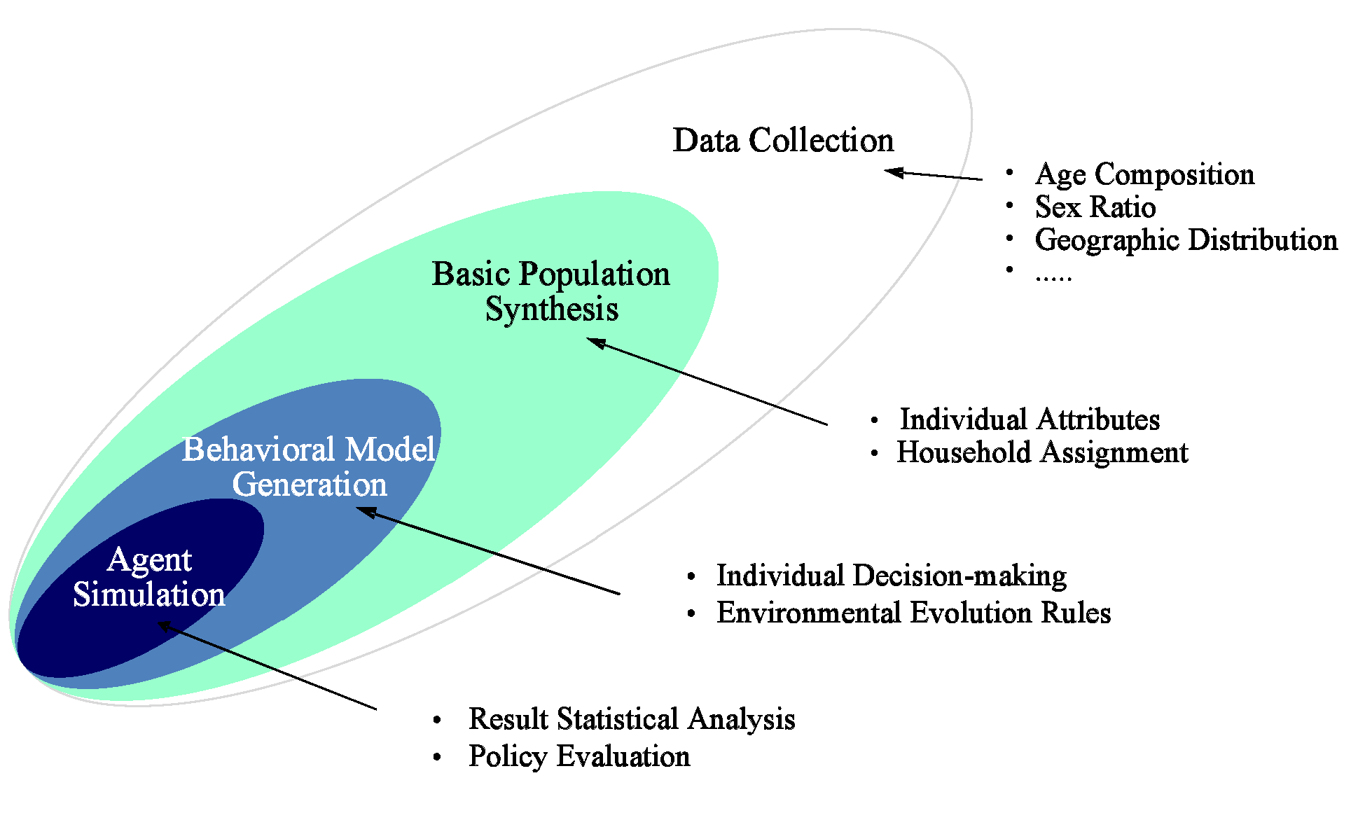
Figure 1. Agent Modeling in Population Research

Population Database Synthesis

3.1

As aforementioned, hybrid agent-based population still needs traditional synthetic population as its initial individual data to launch the subsequent agent interaction. In other words, all the population synthetic techniques in micro-simulation continue to play a critical role in hybrid agent-based population. Based on the types of the input data source, two kinds of synthetic methods can be summarized from current literature: sample-based methods and sample-free methods.

Sample-Based Methods

3.2

Historically, sample-based methods are a standard and fundamental approach for building synthetic population. The input data source usually consists of an aggregate dataset covering the whole target population and a small proportion of original disaggregate sample (Simpson & Tranmer 2005). The typical aggregate data, such as the Summary Files (SF) and Standard Type File 3A (STF-3A) in the U.S, or the Small Area Statistics (SAS) in the UK, includes a set of marginal distributions for specific population characteristics. The disaggregate data, such as the Public Use Microdata Samples (PUMS) in the U.S. and the Sample of Anonymized Records (SAR) in the UK, shows full household and personal details. In population synthesis, the distributions and characteristics provided by disaggregate data are referred to as target and control variables. The disaggregate sample is treated as a seed. The principal task of the synthesis algorithm is to generate an individual dataset in full compliance with the aggregate and disaggregate information. In other words, the synthesis process must generate a population list and its corresponding instances conformed to the aggregate characteristics, with each member containing the attributes associated with the aggregate and actual data input (Zhao et al. 2009) (Figure 2). For decades, sample-based methods have drawn continuous research attention.

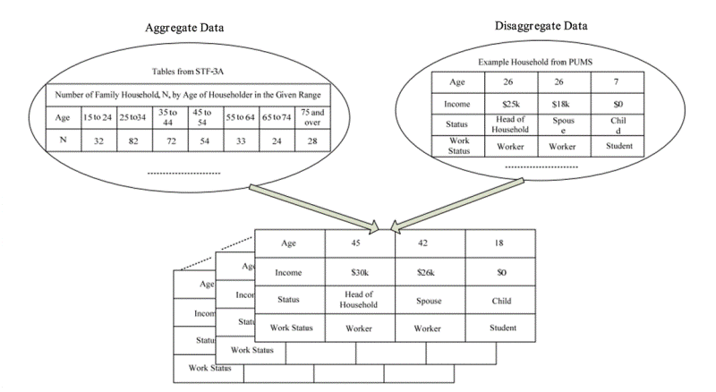
Figure 2. Population Synthesis with Aggregate and Disaggregate Data (Zhao et al. 2009)

Synthetic Reconstruction

3.3

Synthetic Reconstruction (SR), first published in Wilson & Pownall (1976), is the most important and extensively used method in population synthesis. The foundation of this method is the Multiway Table (MT), which holds the conditional probability of the demographic features. If the population contains n attributes, the MT is an \(n\)-dimensional table that includes the overall population scale along with all possible combinations of attributes and related information. However, excluding a few exceptions such as Switzerland, where the complete census can be acquired for research, the original MT in a studied area is almost never available. The central task of Synthetic Reconstruction therefore, becomes the MT estimation and the individual attributes determination, called "Fitting" and "Allocation", respectively (Bowman 2004).

3.4

In the "Fitting" phase, the MT is calculated using the Iterative Proportional Fitting (IPF) method. First proposed by Deming & Stephan (1940), IPF has seen various extensions and become one of the most widely used algorithms (Mosteller 1968; Ireland & Kullback 1968; Fienberg 1970; Csiszár 1975). The input disaggregate data is used to initialize the MT, with the underlying assumption that the sample represents the true correlation structure among the attributes. Among all the tables that satisfy the marginal constraints, the result that IPF yields is the one that most resembles the initial one. Algorithm 1 shows the pseudo code for IPF algorithm (Norman 1999; Speed 2005; Huang & Williamson 2002).

Table 1: The Overall Table to Be Estimated
Attr. \(j\) Attr. \(i\)	\(j=1\)	…	\(j\)	…	\(j=s\)	Marginal Sum
\(i=1\)	\(m_{11}\)	…	\(m_{1j}\)	…	\(m_{1s}\)	\(N_{1 \bullet}\)
…	…	…	…	…	…	…
\(i\)	\(m_{i1}\)	…	\(m_{ij}\)	…	\(m_{is}\)	\(N_{i \bullet}\)
…	…	…	…	…	…	…
\(i=r\)	\(m_{r1}\)	…	\(m_{rj}\)	…	\(m_{rs}\)	\(N_{r \bullet}\)
Marginal Sum	\(N_{\bullet 1}\)	…	\(N_{\bullet j}\)	…	\(N_{\bullet s}\)	\(N\)

Table 2: Sample Table
Attr. \(j\) Attr. \(i\)	\(j=1\)	…	\(j\)	…	\(j=s\)	Marginal Sum
\(i=1\)	\(n_{11}\)	…	\(n_{1j}\)	…	\(n_{1s}\)	\(n_{1 \bullet}\)
…	…	…	…	…	…	…
\(i\)	\(n_{i1}\)	…	\(n_{ij}\)	…	\(n_{is}\)	\(n_{i \bullet}\)
…	…	…	…	…	…	…
\(i=r\)	\(n_{r1}\)	…	\(n_{rj}\)	…	\(n_{rs}\)	\(n_{r \bullet}\)
Marginal Sum	\(n_{\bullet 1}\)	…	\(n_{\bullet j}\)	…	\(n_{\bullet s}\)	\(n\)

Algorithm 1 Iterative Proportional Fitting Algorithm

Input:

Sample Table;

Overall Table (Marginal Sum Known);

Output:

Calculated Overall Table;

1: repeat

2: Update the elements by row according to

\(m_{ij}^\prime=n_{ij}(m_{i\bullet} / n_{i\bullet})\);

3: Update the elements by column according to

\(m_{ij}^{\prime\prime}= m_{ij}^\prime (m_{\bullet j}/m_{\bullet j}^\prime)\);

4: until Iteration Stops

3.5

The IPF method can only deal with one census block (also called "zone" in some references). However, as shown in Figure 3, a Public Use Micro Area (PUMA) in American census contains several basic blocks. Thus joint statistics estimated by the classical IPF are prone to being inconsistent with those in PUMS (Hobeika 2005). A two-step IPF Procedure is proposed as a simple improvement, and is first used to generate population database from the STF-3A and PUMS of 1990 census (Beckman et al. 1996). This method is later applied in the TRANSIMS system (Smith et al. 2005). Based on the IPF convergence proved by Pukelsheim & Simeone (2009), non-convergence only occurs when a row or column has all zeroes while the corresponding marginal sum is non-zero in Table 2.

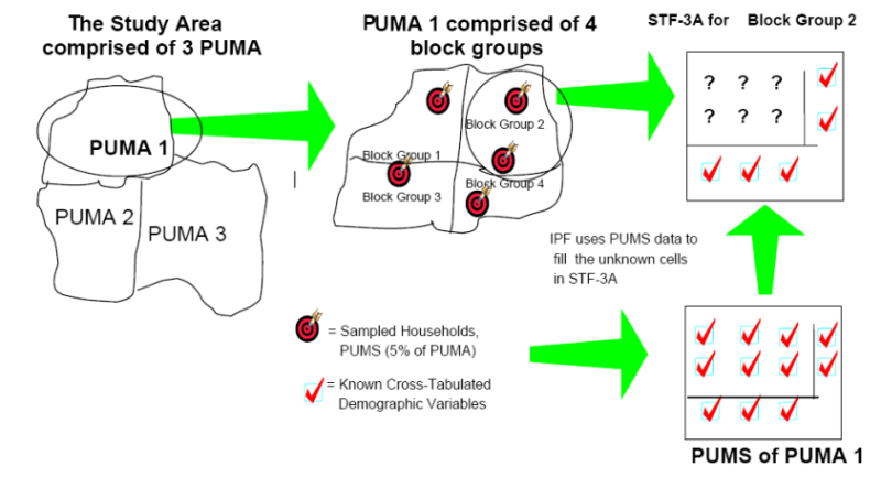
Figure 3. Relationship Between PUMA and Census Block

3.6

While the "Fitting" is the stage that calculates aggregate properties on the target population, the "Allocation" can be regarded as a disaggregation process. Currently, only limited work has been reported on the "Allocation" stage, which generally involves the following tasks (Bowman 2009).

1. Adjust the cell values obtained from IPF in MT as integers;
2. Choose the group or family for each individual according to population distribution;
3. Modify the household geographical information under some specific conditions.

3.7

Among the three steps, the second one plays the central role. Auld used a complex formula to compute agent group selection probability, and showed that the individual marginal probability matched the fitting result well (Auld & Mohammadian 2010). Monte Carlo is another household selection method for agents. In this approach, each family member comes from the qualified population subset, which ensures that the marginal probabilities at family and individual levels are consistent with the fitting results (Pritchard & Miller 2009). Srinivasan presented a deterministic group selection method, which first creates the fitness of agents under the household and individual constraints, then selects the agent with the largest fitness as a family member. The process iterates until the fitness decreases to zero. However, the major issue with this approach is the slow convergence (Srinivasan et al. 2008).

3.8

Several population databases have been generated by synthetic reconstruction. Using the 2000 Switzerland census data, Frick obtained the Zurich basic population through the IPF algorithm and Monte Carlo method. The demographic variables were gender, age, work status, and vehicle ownership, etc. The distribution accuracy was also given (Frick et al. 2004). Because the traditional IPF method cannot solve zero elements and is unable to control the attributes distribution at the household and individual level, Guo offered an improvement on Beckman's method so that the synthetic population was closer to the actual one (Guo & Bhat 2007). The approach was later applied in the population synthesis of the Dallas/FortWorth region in the U.S. In addition, Pritchard and Auld introduced the Sparse List Data and Automatic Category Reduction method, also with the intention of overcoming the problem of zero elements (Pritchard 2008; Auld & Mohammadian 2008). Ye proposed an Iterative Proportional Updating (IPU) algorithm, which runs multiple IPF's in parallel and synthesized individuals and groups simultaneously (Ye et al. 2009). The concept of dynamic artificial population was developed in Zhao et al. (2009) and Ballas et al. (2005a) to take into account population evolution. A simulation system—SimBritain was presented and the modeling and calibration methods for dynamic population were discussed in detail. It also simulated population evolution to the year 2021 from the 1991 British SAS and BHPS (British Household Panel Survey) data. Other typical synthetic population systems are PopSynWin (Auld & Mohammadian 2010, 2008), ILUTE (Pritchard & Miller 2009; Pritchard 2008; Salvini & Miller 2005), PopGen (Ye et al. 2009), FSUMTS (Srinivasan et al. 2008; Srinivasan & Ma 2009), CEMDAP (Guo & Bhat 2007; Pinjari et al. 2006), ALBATROSS (Arentze et al. 2007), etc.

Table 3: RTI Agent-Based Individual Attributes
person_id	490490014021_391_1	490490014021_391_3	…
hh_id	490490014021_391	490490014021_391	…
pnum	1	3	…
age	42	16	…
sex	2	1	…
school_id	< Null >	490081000459	…
work_id	4904900140100240	4904900140200163	…
xcoord	−1319560.00475	−1319560.00475	…
ycoord	252560.73722	252560.73722	…
lat	40.25134	40.25134	…
long	−111.668978	−111.668978	…

Table 4: RTI Household Attributes
hh_id	490490001011_0	490490001011_1	…
persons	4	2	…
hinc	66000	131250	…
p18	1	0	…
wif	4	3	…
xcoord	−1330069.28828	−1330092.56251	…
ycoord	272413.77702	273035.26643	…
lat	40.411208	40.416684	…
long	−111.831806	−111.833349	…

3.9

One of the most valuable databases was created by the Research Triangle Institute (RTI). Using IPF and other theories, RTI produced the population data of the year 2000 for 50 states and the District of Columbia in the U.S. in 2007 and 2009 (Wheaton et al. 2007, 2009), respectively. The agent-based population adopted American census TIGER (Topologically Integrated Geographic Encoding and Referencing) data, SF3, and PUMS as the input. The results include several common attributes as well as the household and school variables. The entire generation process consists of four steps:

1. Generate basic family and population data;
2. Allocate schools for agents;
3. Allocate work places for agents;
4. Generate the rest of the population.

3.10

Individual and family samples are shown in Table 3 and Table 4.

Combinatorial Optimization

3.11

Research and applications of Combinatorial Optimization (CO) method for population synthesis have yet come to full fruition, which leads to much fewer published works than those for Synthetic Reconstruction. The most cited results in the field come from the National Center for Social and Economic Modeling (NATSEM) at University of Canberra, Australia (Williams 2003; Hellwig & Lloyd 2000; Melhuish et al. 2002; King et al. 2002; Harding et al. 2004). Another important contribution from NATSEM is the comparison of SR and CO methods. While it has been found that both of them can generate reliable micro-demographic data, CO holds the edge over SR in the department of smaller deviation (Huang & Williamson 2002). However, it must be noted that this comparison does not consider the scale change in input sample and aggregate data. Additional research has been reported to address the robustness of the two methods with different inputs (Ryan et al. 2009).

Algorithm 2 Combinatorial Optimization Algorithm

Input:

Overall Sample;

Distribution Table;

Output:

Population Dataset;

1: Divide the studied area into several regions;

2: for each region \(A\): do

3: Extract a random sample adapted to the regional scale as the initial population \(P\);

4: Calculate the fitness \(F\) of the initial dataset \(P\);

5: If \(F\) reaches the stop condition, \(P\) is stored as the output population of \(A\), go to 2;

6: Exchange two random individuals from P and the Overall Sample respectively;

7: If \(F\)(before exchange) > \(F\)(after exchange), let \(P =P\)(before exchange); else, let \(P =P\)(after exchange);

8: end for

3.12

When using CO to generate population, it is essential to divide the studied area into several mutually exclusive regions similar to the census blocks or traffic analysis zones. After the attributes set specified, a survey sample of the studied area is produced. The sample consists of the attributes set (called the overall sample) and a statistical investigation table of each region that contains part of the attributes (called the distribution table). For instance, if the population attributes include gender, age, and height, then the overall sample must entail the three attributes values and the distribution table should contain at least one attribute.

3.13

The aim of Combinatorial Optimization is making the attributes values consistent with the distribution table by adjusting the initial population in a particular region. Algorithm 2 illustrates this process. First, a subset adapted to the scale of the target region should be extracted from the overall sample as the initial population. Next, one or more attribute statistics are chosen as the fitness measurement. The fitness of the initial population is then computed. After that, two records are randomly switched from initial dataset and the overall sample, and the fitness is re-calculated. The process repeats until the fitness reaches a certain threshold, and the final dataset is the population of the region. Population of other regions can be generated in the same fashion.

3.14

In general, the Modified Overall Relative Sum of Squared Z-Score (\(\mathrm{RSSZ}_{\mathrm m}\)) is preferred to measure the population fitness in Algorithm 2 (Huang & Williamson 2002). For a specified region, it can be expressed as

$$ \mathrm{RSSZ}_{\mathrm m} = \sum_k \sum_i F_{ki} (Q_{ki}-E_{ki})^2 $$

(1)

where

$$ F_{ki} = \left\{ \begin{array}{cl} \left( C_k O_{ki} \left( 1-\frac{O_{ki}}{N_k}\right) \right)^{-1}, & \quad if~O_{ki} \neq 0;\\ 1/C_k , & \quad if~O_{ki} = 0.\\ \end{array}\right. $$

\(O_{ki} \) is the \(k\)-th observed attribute of the \(i\)-th individual in the population subset. \(E_{ki}\) is the \(k\)-th attribute expectation of the \(i\)-th individual in the overall sample (already known). Nk is the number of individuals that contain the \(k\)-th attribute. \(C_k\) is the 5% \(\chi^2\) critical value of the \(k\)-th attribute. When the population fitness of a region is in full compliance with that of the overall sample, RSSZm will decrease to zero. In practice, \(\mathrm{RSSZ}_{\mathrm m}\) has the following advantages:

1. \(\mathrm{RSSZ}_{\mathrm m}\) is a fitness measurement independent of the population scale. In other words, we can directly compare two fitnesses even if they are derived from distinct groups.
2. In essence, \(\mathrm{RSSZ}_{\mathrm m}\) is the sum of the fitness of each attribute and weighs them equally.
3. \(\mathrm{RSSZ}_{\mathrm m}\) has its clear meaning. When \(\mathrm{RSSZ}_{\mathrm m}\) is less than 1.0, it is believed that the synthetic population is consistent with the attribute table.

3.15

Several other statistical indicators such as the Freeman-Tukey statistics have been used in the fitness computation as well (Voas & Williamson 2000, 2001).

3.16

Note that both Synthetic Reconstruction and Combinatorial Optimization can generate synthetic population with increasing high accuracy as the scale of the input disaggregate sample grows. However, the speeds of convergence are different. When taking into consideration the sample acquisition cost and the population accuracy, it is recommended that appropriate sample scales for CO and SR are 5% and 2.5%, respectively (Ryan et al. 2009).

Sample-free Methods

3.17

Different from their sample-based counterparts, sample-free methods are a synthetic technique that have only emerged in recent years. Motivated by the need to reduce dependence on small proportion of disaggregate sample, these methods aim to create synthetic population by using only the aggregate data. In other words, marginal distributions of all the population characteristics are the only input in this approach. However, it should be noted that sample-free methods do not exclude the use of disaggregate sample when it is available. Because the original aggregate data published by Bureau of Statistics or other agencies most likely do not contain all combinations of the characteristics, we need to supplement the missing conditional probabilities, which can be extracted from the sample or computed from other data sources. Actually, disaggregate sample may be used to give good estimate of the distributions provided it conforms to the entire population very well. Two typical sample-free methods have been elucidated in the literature.

Sample Free Fitting

3.18

Sample Free Fitting builds households by assigning appropriate individuals as their members (Gargiulo et al. 2010; Barthelemy & Philippe 2013). Based on several discrete and continuous optimization procedures, this method has higher flexibility in terms of data requirements. In the synthetic process, an individual pool with the scale of target population needs to be generated based on the marginal distributions computed from various data sources at the individual level. Then, a proper list of "empty" households is constructed in sequence by using the distributions at the household level. Appropriate members are selected from the individual pool with their roles assigned as either a household head or a partner. The initial individual set is shrinking progressively during this selection process. The iterations end when all households are fulfilled or the generator fails to find a particular household member due to exhaustion of individuals or lack of suitable individuals in the pool. However, slight distinctions also exist between Gargiulo's and Barthelemy's research. In Barthelemy's work, if there is no appropriate individual in the current set, the generator will choose a member from the households already created, whereas Gargiulo restricts the selection in the set only.

3.19

The synthetic procedure of Sample Free Fitting involves various complicated and hierarchical fitting steps (for each aggregation level where the data is available). We are therefore convinced that it deserves an introduction , in this review, along with entropy maximization, tabu search, and various ad hoc matching rules. Generally speaking, this approach has overcome a strong limitation of the sample-based method. However, it does not guarantee the simultaneous matching of the control totals for both households and individuals. The method was applied to synthesize Belgian population at the scale of 10,000,000 with limited attributes, but it remains unclear whether it can be successfully extended to other cases.

Markov Chain Monte Carlo Simulation

3.20

Markov Chain Monte Carlo (MCMC) methods are computer-based techniques to simulate random drawing of a dependent sequence from very complicated stochastic models. When applied to population synthesis, they are referred to as the simulation-based approach (Farooq et al. 2013). The idea of creating population by directly drawing from a probability distribution can be traced back to TORUS, which simulated the households' location choices in Toronto area, Canada (Miller et al. 1987). In Farooq's method, the individuals are characterized by a set of attributes \(X=(X^1, X^2, \cdots, X^n)\). The problem is defined as developing a synthesis procedure to create a synthetic population as if we were drawing from the actual population with the unique distribution \(\pi _X(x)\). Meanwhile, the synthesis procedure must also ensure that the empirical distribution \(\pi_{X^\prime}(x^\prime)\) of the synthetic population is as close to \(\pi_X(x)\) as possible. Usually, the actual distribution \(\pi_X(x)\) is hard to access, and we can only get some partial views from various types of available data sources.

3.21

The MCMC method is composed of two parts: Gibbs sampling and population realization. The Gibbs sampling uses the conditional distribution \(\pi (X^i | X^j=xj,\ \mathrm{for}\ j=1, \cdots, n \& j\neq i)= \pi;(X^i | X^{-i})\), for \(i=1, \cdots, n\) to simulate \(\pi_X(x)\). The crucial operation is to prepare the conditional distributions of the attributes using all the available data. Generally, the conditional distributions can be categorical sum of each attribute from the census statistics or the disaggregate input data like PUMS. Parametric models are also used to construct the conditional distributions. The flexibility of using such models is that the data from various sources can be combined to estimate the parameters. It should be mentioned that the full conditional distribution of an attribute over all the other attributes may not be available. Suppose that in \(\pi(X^1 | X^{-1})= \pi(X^1 | X^{(2\ldots k)}, X^{((k+1)\ldots n)})\), only the incomplete conditional \(\pi(X^1 | X^{(2\ldots k)})\) is available. We can assume the conditional independence of \(X^1\) on \(X^{((k+1)\ldots n)}\) when \(\pi( X^1 | X^{(2\ldots k)})\) is given. Therefore, \(\pi(X^1 | X^{-1})= \pi(X^1 | X^{(2\ldots k)})\). In the worst case where only marginal distributions are available, we have \(\pi(X^1 | X^{-1})= \pi(X^1)\). Some other information such as the domain knowledge about the incomplete part of the conditional can also help to construct full conditionals.

3.22

Based on the full and consistent conditionals, the Gibbs sampling will eventually reach a stationary state after it runs for an extended amount of iterations. At this state, it would be as if the drawing is from the actual population, so the synthetic population can be realized by simply drawing individuals with a total number equaling the scale required. In this way, two populations generated will have similar statistics. The distribution of the synthetic population will be close to \(\pi_X(x)\), the degree of closeness depends on the quality of the input data.

3.23

A comparison of the simulation-based approach and Synthetic Reconstruction using the actual Swiss census is given by Farooq et al. (2013). The standard root mean square error shows that the simulation-based approach outperforms the SR. One highlight of MCMC is the integrated partial views of the joint distributions of the actual population attributes from various data sources. Meanwhile, different from SR, which is limited to discrete attributes only, the MCMC can deal with both discrete and continuous attributes, or a mixture of both. However, the MCMC approach also has flaws: When the data source and the domain knowledge are inconsistent, the Gibbs sampling may never reach a unique stationary state. Further study is needed to address this problem. Because the MCMC method is deemed relatively new, applications are rare.

3.24

Sample-based approach is still the primary method to generate population in most existing simulation systems. Specifically, IPU, derived from IPF, provides a parallel synthetic process for individuals and households, which is more suitable for large scale computation. In contrast with the sample-based method, sample-free method is less data demanding. However, it requires more data preparation due to the need of extracting marginal distributions from various data sources. Lenormand & Deffuant (2012) assessed the performance of the IPU and Sample Free Fitting. They concluded that the Sample Free Fitting gave better accuracy of the distributions at both the household and individual levels, while the IPU method depended much on the quality of the disaggregate sample. The execution time on a single desktop machine was almost the same. Though these conclusions need further investigations, their work has confirmed the possibility of initializing solid agent-based population simulation without any disaggregate sample.

Agent Model Generation

4.1

When the initial population is created, we need to generate the micro behavioral model for each kind of agent. An agent is usually denoted as a hardware or software-based computer system with the following features (Zhao 2009):

1. Autonomy. Agents can control the behavior and internal state themselves, and are not directly influenced by others for their decision-making or belief. As a basic property, autonomy is an important feature that separates an agent from other abstract entities.
2. Reactivity. Agents can perceive the environment and respond to the stimulus in time.
3. Social Ability. Agents can perform interaction and exchange information. In a multi-agent system (MAS), the behavior of an agent is not isolated but social. Therefore, collaboration is essential to achieving a mutual goal. Social ability is the foundation of the agent collaboration and learning.
4. Learning Ability. Agents can observe their own actions as well as the behaviors of others. They will learn, evolve, and improve their decision-making ability and belief. Learning ability reflects the intelligence of agents.
5. Proactivity. Agents can not only respond to the environmental changes, but also take initiatives to achieve their goals in specific cases.
6. Mobility. At selected times and places, agents can be mobile in the network.

4.2

Agent-based modeling can trace its origin to Neumann & Burks (1966). It aims to simulate the interaction between individuals with autonomy and study the global characteristics emerged from bottom-up. This manifests the principle that the simple behavior rules can lead to complex global phenomena.

4.3

In general, three distinct kinds of agent models in artificial intelligence have been carefully studied, which are: reactive agents, deliberative agents, and compound agents.

4.4

Research on reactive agents was started by Brooks and Agre (Brooks 1986; Agre & Chapman 1987). This type of agents attaches great importance to its response to environment and the intelligence gained from interactions with its peers (Ferber 1994). Brooks believed that the intelligent behavior can be realized through irritability without considering or even understanding the environment. Maes summarized three advantages of the reactive model (Maes 1990).

1. Interactions between the agent and the environment are dynamic. Agents need to be able to respond to emergency when they have little time to plan. The reactive model meets this requirement well.
2. Reactive agent can reduce the communication load between various modules.
3. Reactive agent is suitable for processing data source.

4.5

Figure 4 shows the structure of reactive agents. Two extensively used reactive agent structures are as follows.

1. Situated-Action Rules (Suchman 1987). This structure establishes the interactive rules by mapping the environmental states with behaviors. Flat and nested rules are two classic patterns. The flat pattern, which is the most comprehensively used, arranges all rules at the same level and only one rule can be activated at a time. The nested pattern organizes the rules in different priorities. Agents can calculate the cost when several rules are activated simultaneously. In fact, the nested pattern is a simple but effective multi-parallel information processing structure.
2. Augmented Finite State Machine (AFSM) (Brooks 1990). AFSM contains internal states, which significantly enhance their abilities to model complex behaviors. When the input signal exceeds a certain threshold, agents will execute a corresponding action.

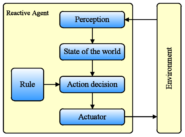
Figure 4. The Model of Reactive Agent

4.6

Deliberative agents contain an internal rational model and are interactive with the environment through their behavior plan. The intelligence of this type of agents is shown in its ability for planning, reasoning, and striving for goals. Figure 5 gives its structure. Commonly used deliberative agent models include:

1. SOAR: Similar to expert system, SOAR (State, Operator, And Result) is based on the "If…,
2. Then…" reasoning.
3. BDI: It is built on the concept of Belief-Desire-Intention where belief stores the awareness of its world, desire records its goals, and intention describes the procedures that agents need to take to achieve specific goals.

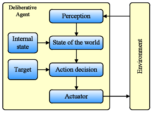
Figure 5. The Model of Deliberative Agent

4.7

Based on the BDI, modified models for particular applications are proposed. For example, InterRAP expands the BDI to a three-layer structure that includes a World Model (the knowledge of its environment), a Mental Model (the understanding of itself), and a Social Model (the knowledge of other agents). The World Model uses reactive architecture, while the Mental Model and Social Model adopt deliberative architecture.

4.8

Compound agents integrate the strengths of both reactive and deliberative models. They develop a goal-oriented behavior plan by deliberation. Specifically, a macro-plan is decomposed into several micro-plans to be carried out by the modules of micro behaviors, and the micro-plans are mapped into a series of micro-actions to influence the environment (Figure 6).

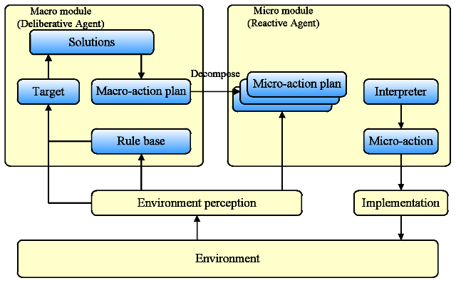
Figure 6. The Model of Compound Agent

4.9

Reactive agents have relatively simpler architecture but lower intelligence than deliberative agents. In addition, they generally do not have the learning ability as the other types of agents. Nevertheless, as simple as single reactive rule seems to be, large quantities of reactive agents can still trigger sophisticated dynamics. Deliberative agents can model human intelligence more accurately, yet they may require more complicated reasoning mechanism and are likely to be computationally overwhelming. Therefore, after the basic population data is generated, selecting a proper agent model is vital for the population interaction and the succeeding simulation. The core of constructing an agent is formulating the action and reaction rules to counterparts and environment from its behavior. In this way, the feedback between individual and population system can be conveniently established.

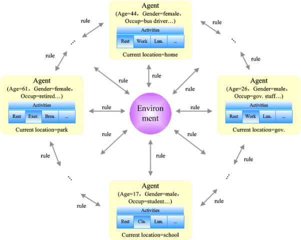
Figure 7. Agent, Environment, and Rules in Artificial Population

4.10

Two successful cases are John Conway's Game of Life (Gardner 1970) and Schelling's Segregation model (Schelling 1971). In Conway's life game, individuals may die due to congestion or isolation, therefore survival and death of individuals depend on the local density of agents "alive". Schelling's Segregation model suggests that segregation between cities still exists even if the society is quite tolerant. Billari introduced agent mechanism into the population research and proposed the agent-based computational demography (Billari & Prskawetz 2003). Figure 7 elaborates the elements of agent-based artificial population systems, which are agents, environment, and rules (Zhao 2009). Each agent, being the "person" in artificial population systems, has its own internal states as well as rules. It changes itself with external environmental transformation. Environment, which can be actual or virtual, is the place where the agents reside. Virtual environment is generally a network that agents perform their activities. Rules are the interaction norms or steps between agents or organizations.

4.11

After agent models are determined, some update rules for internal attributes and environment are essential. One relatively simple way is using existing rules with parameters calibrated by the empirical data. Some basic rules are as follows:

1. Age composition:

   $$\sum_{i=1}^N p_i=1 $$

   where \(N\) is the number of intervals and \(p_i\) is the agent number in the \(i\)-th interval.

2. Gender composition:

   $$p_{\rm male}+p_{\rm female}=1. $$

3. Marriage composition:

   $$p_{\rm married}+p_{\rm unmarried}=1. $$

4. Growth rule: the age increases by one.
5. Marriage rule: an agent cannot get married until a certain age; only a pair of agents with opposite genders can marry with a probability; the couple should not be related.
6. Fertility rule: only married females can be pregnant; the pregnant age is usually between 15 and 49; the gender of the child is randomly determined.
7. Death rule: the agent will exit the system when its age reaches a threshold (Huang 2008).

4.12

Other particular rules can be added or deleted to study the decision process and influences for a specific problem.

4.13

Table 5, 6 and 7 list the prominent applications of population studies using agent technology. Most of these applications, due to their complexities, adopt the reactive agents because of the heavy computation needed for deliberative agents.

Table 5: Applications in Population Studies: Spatial Demography
Researcher(s)	Research Subject	Methodology	Findings
Spatial Demography: Spatial movement and distribution of agent with different decision rules based on Schelling model
Heiland (2003)	Migration patterns from east to west in Germany	Migrations are triggered by unemployment, income inequality, migration cost, and other factors. Agents are heterogeneous in terms of residence and mobility.	Unemployed agents migrate more easily, and they tend to be close to the regions that require skilled labors.
Benenson et al. (2003)	Residential mobility in Yaffo area of Tel-Aviv	For three different ethnic groups (Arab Christians, Muslims and Jews), the agents first decide their likelihood of migration, then choose from a set of randomly selected vacant houses the most attractive one.	The result is quite consistent with the reality, especially after the vacant houses ranking is included.
Castle & Crooks (2006); Crooks (2006)	The spatial distribution of agents	Introduce Geographic Information System (GIS) information into the agent model.	The spatial representation of agents are expanded from a two dimensional lattice to GIS.
Crooks et al. (2008)	Agent behavioral simulation	Introduce the residential location model, the pedestrian evacuation model, and the land-use macro-structure in London's transportation systems.	Exhibit the complex micro- and macro phenomena through the interactions of individuals.
Lenormand et al. (2012); Simini et al. (2012); Gargiulo et al. (2012)	Agents mobility patterns	Use Monte-Carlo simulation to generate commuting networks according to the statistics of commuters in different regions of France, UK and Germany.	Find new universal models for mobility and migration patterns that contain fewer parameters.

Table 6: Applications in Population Studies: Family Demography
Researcher(s)	Research Subject	Methodology	Findings
Family Demography: Decision-making process.
Todd (1997)	The mate selection	Study the optimal spouse selection algorithm in a "simple" agent model.	Find a faster method than the optimal algorithm, which cannot be derived from analysis.
Todd & Billari (2003)	The formation of marriage	Simulate the unilateral and mutual spouse selection in an agents group by combining the selection mechanism and marriage patterns.	Heterogeneity is essential for generating the overall characteristics from individual desires.
Billari et al. (2003)	Change of the marital age	Regulations contained in the agent can be passed on to children as constraints. A pair of agents can get married only when their ages are in a certain range.	Regulations about marital age can be enforced in many generations.
Billari et al. (2008)	Marriage model research based on social interaction	Two important factors concerning the social structure and form of marriage are considered: partner accessibility and desire for marriage. The former comes from potential partners and is modeled by the network scale and spouse search, while the latter directly considers the impact of marriage: social pressure and the marriage experience of others.	The risk of marriage is from microscope, but robust to parameter changes.
Hills & Todd (2008)	Spouse, marriage and divorce model	Agent searches for spouse according to similarity with a relaxation of age. When an agent finds an individual more similar than the current spouse, divorce will occur.	The model is able to predict the patterns of marriage and divorce under different cultures.

Table 7: Applications in Population Studies: Historical Demography
Researcher(s)	Research Subject	Methodology	Findings
Historical Demography: Known as artificial societies, mainly studies the phenomenon caused by the changes of micro-behavior or environment
Epstein & Axtell (1996)	Dynamic evolution of society	The agent is put in the "sugar environment", and a simple survival rule is set up: in the visible range, agent will move to the position with more sugar which is necessary for survival and consumes the sugar according to the metabolism rate.	Complex behaviors such as group formation, culture, war, trade and migration are the direct consequences.
Dean et al. (2000); Axtell et al. (2002)	Evolution of ancient human	Study the maize production per hectare with the assumption that the minimum simulation unit is a single family and some attributes (such as age, size, composition, the corn stock) are defined. The nutrition requirements decide the family migration patterns	Simulation accurately reproduces the main features of population changes in Anasazi such as tides, internal migration patterns, and the final decline of population.
Ewert et al. (2003)	The analysis of modern European urban mortality crisis	A modern town is constructed in Java environment. Three types of agents (merchant, artisan, and labor) are included with their utility and profit maximized. Another agent which represents the local government is introduced to intervene in the market and the social structure according to a specific function.	There emerges a variety of negative tactics that are close to what would occur in reality.
Konig et al. (2003)	The emergence of stratum and social collaboration	The individual can cooperate with others, and acts as an information hub to seek the best place to get food.	The model is better for realizing sustainable development than the isolated one.
Murphy (2003)	The feedback mechanism of agents	Compare models with or without feedback mechanism.	Agent-based model may improve the existing methods for studying virtual society and sustainable population.
Zhao (2009); Miao (2007)	Transportation oriented agent model	Consider the social class, age distribution, gender, occupation characteristics etc.	A variety of complex traffic scenarios "emerged".

Conclusions and Future Work

5.1

This paper provides a detailed review of the latest development concerning two aspects of hybrid agent-based population. We first elucidate the framework of hybrid agent modeling for population study. Current approaches for initial population synthesis and typical agent models, which form the foundation of hybrid agent-based population simulation, are then reviewed in detail.

5.2

Though showing promising advantages over the traditional population research methods, the agent-based approach also faces some significant challenges (Chattoe 2001; Morand et al. 2010):

1. Modeling in social sciences usually concentrates on very specific aspects of social behavior. For example, to apply the standard statistical analysis, which assumes a "static" casual relation between variables, to social studies, we have to identify some direct causes for the behavior of interest while treating all other factors as exogenous. Unfortunately, the casual relevance as well as irrelevance, cannot be transplanted seamlessly to agent-based models. We should distinguish between causal factors in social actions and societal properties (called the structuring factors) very carefully. Particular social behavior must be first modeled as light-weighted as possible so that adequate representation of relevant structuring factors from broader social environment can be added later.
2. Current social theories, in a sense, do not seem to offer satisfactory guidance for agent-based modeling. One example is the aggregate statistical regularities: though widely used by social scientists to predict average behaviors, they tell us almost nothing reliable about individuals and thus have limited value for agent behavioral models. Also, conventional agent theories assume that agents are fundamentally homogenous, while agents in population simulation are inherent heterogeneous. Consequently, the process of agent modeling cannot rely on the existing theories because they are either excessively restrictive or empirically unrealistic.
3. Social actions always take place in a certain social context, i.e., the time and place of the occurrence. Therefore, spatial and temporal information are integral part of agent behavior and essential to agent decision making. However, to include this context in modeling is likely to cause considerable non-linearity and clustering to information transfer, and might be seen as contradicting the idea of having light-weighted models initially.
4. Simulating the agent with cognitive complexity in a more realistic way may be another extremely difficult task. It involves storing relevant information and transforming information to action. If we postulate very simple decision making models, the majority of information will either be discarded or regarded as mere noise. If we take social interaction seriously, we have to study how agents deal with all the information they receive.
5. Finally, in many Multi-Agent Systems, not much thought has been given to the data needed to calibrate the agent model and how to collect them. At present, interview is the dominant measure for soliciting information about how people make decisions. However, if we want to further explore human decision making rather than making assumptions from our theories, new kinds of data as well as acquisition technology needs to be developed.

5.3

It should be noted that raising the above difficulties is not intended to downplay the merits of agent-based or other existing approaches. On the contrary, both the agent-based models and their traditional statistical and mathematical counterparts have advantages as well as challenges in accurately representing social behaviors.

5.4

Hybrid agent-based population is still a developing field. Many promising directions require rigorous investigation. Here we only introduce two of them. First, agent-based models investigate the decision making mechanism more deeply and insightfully than standard micro-simulation methods. On the other hand, micro-simulation is supported by substantial data collection, representation, estimation, and validation in an empirical setting. Thus, hybrid agent-based population simulation, which combines agent technology with basic synthetic population data, can lay a solid foundation for social simulation. However, to the best of our knowledge, few studies have been published. The temporary lack of research may be attributed to two reasons: first, the scarcity of original census data has undoubtedly hindered the construction of simulation systems by researchers; second, government employees at Bureau of Statistics who have full access to census might not be equipped with the expertise for designing suitable agent-based models. As the motivation for demography and other distinctive social sciences is to move away from simple models by developing theories of human cognitive and social structure that are adequate to support the understanding of particular behaviors, how to model human decision making process more properly in population simulation may be the next task we need explore. One direct attempt, as it seems, is to use deliberative architecture. But for many problems, such as the construction of internal models, the rapid increase of computations for large scale simulation still poses the biggest challenge and needs to be acutely addressed. Second, though it is debatable whether it is realistic to validate social simulation models, model calibration can hardly be avoided (Chattoe 2001; Ngo & See 2012). Among the calibration approaches that have already been proposed, most of them concentrate on the computational economics (Windrum, et al. 2007; Moss 2008; Fabretti 2011). How can these methods be applied to the demographic simulation is unclear. This might raise another two pertinent problems further. The first problem is connected to the criteria for agent behavioral calibration. If the calibration aims to approximate the reality, its qualitative and quantitative specification needs to be considered. Moreover, introducing other theories (such as the theory of parallel universe) may provide innovative paths for agent-based population study. The second problem concerns the acquisition of the calibration data. This originates from the difficulty of measuring human behavior directly. How to develop this kind of data collection method, or even using other measured data driven approaches to model agent directly, still remains to be addressed.

---

References

AGRE, P. E. & Chapman, D. (1987). Pengi: An implementation of a theory of activity. In: AAAI 87. http://www.aaai.org/Library/AAAI/1987/aaai87-048.php

ARENTZE, T., T immermans, H. & Hofman, F. (2007). Creating synthetic household populations: problems and approach. Transportation Research Record: Journal of the Transportation Research Board 2014(1), 85–91. http://trb.metapress.com/index/2jn0l95n77322626.pdf

AULD, J. & Mohammadian, A. (2010). Efficient methodology for generating synthetic populations with multiple control levels. Transportation Research Record: Journal of the Transportation Research Board 2175(1), 138–147. http://trb.metapress.com/index/YV4M68361563G413.pdf

AULD, J. A. & Mohammadian, K. & Wies, A. (2008). Population synthesis with control category optimization. Proceedings of the 10th International Conference on Application of Advanced Technologies in Transportation.

AXTELL, R. L., Epstein, J. M., Dean, J. S., Gumerman, G. J., Swedlund, A. C., Harburger, J., Chakravarty , S., Hammond, R., Parker, J. & Parker, M. (2002). Population growth and collapse in a multiagent model of the Kayenta Anasazi in Long House Valley. Proceedings of the National Academy of Sciences of the United States of America 99 (Suppl 3), 7275–7279.

BALLAS, D., Clarke, G., Dorling, D., Eyre, H., Thomas, B. & Rossiter, D. (2005a). Simbritain: A spatial microsimulation approach to population dynamics. Population, Space and Place 11(1), 13–34. http://onlinelibrary.wiley.com/doi/10.1002/psp.351/abstract

BALLAS, D., Clarke, G., Dorling, D. & Rossiter, D. (2007). Using Simbritain to model the geographical impact of national government policies. Geographical Analysis 39(1), 44–77.

BALLAS, D., Clarke, G.P., & Wiemers, E. (2005b), Building a dynamic spatial microsimulation model for Ireland, Population, Space and Place, 11, 157–72.

BARTHELEMY, J. & Toint, P. L. (2013). Synthetic population generation without a sample. Transportation Science 47(2), 266–279.

BECKMAN, R. J., Baggerly , K. A. & McKay , M. D. (1996). Creating synthetic baseline populations. Transportation Research Part A: Policy and Practice 30(6), 415–429. http://www.sciencedirect.com/science/article/pii/0965856496000043

BENENSON, I., Orner, I. & Hatna, E. (2003). Agent-based modeling of householders' migration behavior and its consequences. Springer.

BILLARI, F. C. & Prskawetz, A. (eds.) (2003). Agent-based computational demography: Using simulation to improve our understanding of demographic behavior. Physica-Verlag.

BILLARI, F. C., Prskawetz, A., Diaz, B. A. & Fent , T. (2008). The "wedding-ring": An agent-based marriage model based on social interaction. Demographic Research 17(59). http://books.google.com/books?hl=en&lr=&id=KDAS4LhPqjMC&oi=fnd&pg=PA59&dq=The+%60%60Wedding+Ring%27%27:+An+Agent-Based+Marriage+Model+Based+on+Social+Interaction&ots=bOSNcddCzM&sig=8TypE4H6_Z62wyeNORo1nvgR38o

BILLARI, F. C., Prskawetz, A. & Furnkranz, J. (2003). On the cultural evolution of age-at-marriage norms. Springer.

BIRKIN, M. & Clarke, M. (2011). Spatial microsimulation models: A review and a Glimpse into the future. Population Dynamics and Projection Methods. Springer, 193–208.

BIRKIN, M. & Wu, B. (2012). A review of microsimulation and hybrid agent-based approaches. Agent-Based Models of Geographical Systems. Springer, 51–68.

BOWMAN, J. L. (2004). A comparison of population synthesizers used in microsimulation models of activity and travel demand. Working paper. http://jbowman.net/papers/2004.Bowman.Comparison_of_PopSyns.pdf

BOWMAN, J. L. (2009). Population synthesizers. Traffic Engineering and Control 49(9), 342.

http://www.jbowman.net/papers/2009.Bowman.Population_synthesizers.pdf

BROOKS, R. A. (1986). A robust layered control system for a mobile robot. Robotics and Automation, IEEE Journal of 2(1), 14–23. http://ieeexplore.ieee.org/xpls/abs_all.jsp?arnumber=1087032

BROOKS, R. A. (1990). Elephants don't play chess. Robotics and Autonomous Systems 6(1), 3–15. http://www.sciencedirect.com/science/article/pii/S0921889005800259

BUILDER, C. H. & Bankes, S. C. (1991). Artificial societies: A concept for basic research on the societal impacts of information technology. Tech. rep., Rand Corp.

CASTLE, C. J. & Crooks, A. T. (2006). Principles and concepts of agent-based modelling for developing geospatial simulations. Working paper 110. Center for Advanced Spatial Analysis, University College London. http://eprints.ucl.ac.uk/3342

CHATTOE, E. (2001). The role of agent-based modelling in demographic explanation. Agent-Based Computational Demography. Physica-Verlag.

CROOKS, A., Castle, C. & Batty, M. (2008). Key challenges in agent-based modeling for geo-spatial simulation. Computers, Environment and Urban Systems 32(6), 417–430. http://www.sciencedirect.com/science/article/pii/S0198971508000628

CROOKS, A. T. (2006). Exploring cities using agent-based models and GIS. Center for Advanced Spatial Analysis, University College London: Working paper 109. http://discovery.ucl.ac.uk/3341/

CSISZAR, I. (1975). I-divergence geometry of probability distributions and minimization problems. The Annals of Probability, 146–158. http://www.jstor.org/stable/2959270

DEAN, J. S., Gumerman, G. J., Epstein, J. M., Axtell, R. L., Swedlund, A. C., P arker, M. T. & McCarroll, S. (2000). Understanding Anasazi culture change through agent-based modeling. Dynamics in Human and Primate Societies: Agent-Based Modeling of Social and Spatial Processes, 179–205. http://books.google.com/books?hl=en&lr=&id=O1LF3icXOLIC&oi=fnd&pg=PA179&dq=Understanding+Anasazi+Culture+Change+Through+Agent-ased+Modeling&ots=ilRmgPisuy&sig=nf4cbCs0Q34BW32XTogvTwuSbeA

DEMING, W. E. & Stephan, F. F. (1940). On a least squares adjustment of a sampled frequency table when the expected marginal totals are known. The Annals of Mathematical Statistics 11(4), 427–444. http://www.jstor.org/stable/2235722

EPSTEIN, J. M. & Axtell, R. L. (1996). Growing artificial societies: Social science from the bottom up. The Brooking Institute Press and MIT Press.

EWERT, U. C., Roehl, M. & Uhrmacher, A. M. (2003). Consequences of mortality crises in pre-modern European towns: A multiagent-based simulation approach. Springer.

FABRETTI, A. (2011). Calibration of an agent based model for financial markets. Highlights in Practical Applications of Agents and Multiagent Systems. Springer Berlin Heidelberg, 89, 1–8.

FAROOQ, B., Bierlaire, M., Hurtubia, R. & Flotterod, G. (2013). Simulation based population synthesis. Transportation Research Part B: Methodological 58, 243–263. http://www.sciencedirect.com/science/article/pii/S0191261513001720

FERBER, J. (1994). Simulating with reactive agents. Many Agent Simulation and Artificial Life 36(6), 8–28.

FIENBERG, S. E. (1970). An iterative procedure for estimation in contingency tables. The Annals of Mathematical Statistics, 907–917. http://www.jstor.org/stable/2239244

FRICK, M., Axhausen, K. W., Axhausen, K. W. & Axhausen, K. W. (2004). Generating synthetic populations using IPF and monte carlo techniques: Some new results. Institute for Transport Planning and Systems, Swiss Federal Institute of Technology, Zurich.

GARDNER, M. (1970). Mathematical games: The fantastic combinations of john Conway's new solitaire game life. Scientific American 223(4), 120–123.

GARGIULO, F., Lenormand, M., Huet, S. & Espinosa, O. B. (2012). Commuting network models: Getting the essentials. Journal of Artificial Societies and Social Simulation 15(2), 6.

GARGIULO, F., Ternes, S., Huet, S. & Deffuant, G. (2010). An iterative approach for generating statistically realistic populations of households. PloS one 5(1), e8828.

GILBERT, N. & Troitzsch, K. (2005). Simulation for the social scientist. McGraw-Hill International.

GUO, Y. J. & Bhat, R. C. (2007). Population synthesis for micro-simulating travel behavior. Transportation Research Record 2014, 92–101.

HARDING, A., Lloyd, R., Bill, A. & King, A. (2004). Assessing poverty and inequality at a detailed regional level: New advances in spatial microsimulation. 2004/26. Research Paper. United Nations University.

HEILAND, F. (2003). The collapse of the Berlin Wall: Simulating state-level east to west German migration patterns. Springer.

HELLWIG, O. & Lloyd, R. (2000). Socio demographic barriers to utilization and participation in telecommunications services and their regional distribution: A quantitative analysis. University of Canberra (NATSEM).

HILLS, T. & Todd, P. (2008). Population heterogeneity and individual differences in an assortative agent-based marriage and divorce model (madam) using search with relaxing expectations. Journal of Artificial Societies and Social Simulation 11(4), 5.

HOBEIKA, A. (2005). Transims fundamentals. Tech. rep., U.S. Department of Transportation. http://tmip.fhwa.dot.gov/transims/transims_fundamentals/ch3.pdf

HUANG, Q. (2008). Continuous age model of mortality. Population Research 32(5), 15–25.

HUANG, Z. & W illiamson, P. (2002). A comparison of synthetic reconstruction and combinatorial optimization approaches to the creation of small-area micro-Data. Working paper, Department of Geography, University of Liverpool. http://pcwww.liv.ac.uk/~william/Microdata/workingpapers/hw_wp_2001_2.pdf

HUET, S., Lenormand, M., Deffuant, G. & Gargiulo, F. (2014). Parameterisation of individual working dynamics. In: Empirical Agent-Based Modeling-Challenges and Solutions. Springer, 133–169.

IRELAND, C. T. & Kullback, S. (1968). Contingency tables with given marginals. Biometrika 55(1), 179–188. http://biomet.oxfordjournals.org/content/55/1/179.short

KING, A., Lloyd, R. & McLellan, J. (2002). Regional microsimulation for improved service delivery in Australia: Centrelink's CuSP model. National Centre for Social and Economic Modeling (NATSEM), University of Canberra.

KONIG, A., Mohring, M. & Troitzsch, K. G. (2003). Agents, hierarchies and sustainability. Springer.

LEBARON, B., Arthur, W. B. & P almer, R. (1999). Time series properties of an artificial stock market. Journal of Economic Dynamics and Control 23(9), 1487–1516. http://www.sciencedirect.com/science/article/pii/S0165188998000815

LENORMAND, M. & Deffuant, G. (2012). Generating a synthetic population of individuals in households: Sample-free vs sample-based methods. arXiv preprint arXiv:1208.6403.

LENORMAND, M., Huet, S., Gargiulo, F. & Deffuant, G. (2012). A universal model of commuting networks. PloS one 7(10), e45985.

MAES, P. (1990). Designing autonomous agents: Theory and practice from biology to engineering and back. MIT press.

MELHUISH, T., Blake, M. & Day, S. (2002). An evaluation of synthetic household populations for census collection districts created using optimization techniques. Australasian Journal of Regional Studies, 8(3), 369. http://search.informit.com.au/documentSummary;dn=028511002039922;res=IELHSS

MIAO, Q. (2007). Design of artificial transportation system based on artience. Ph.D. thesis, Institution of Automation, Chinese Academy of Sciences.

MILLER, E., Noehammer, P. & Ross, D. (1987). A micro simulation model of residential mobility. International Symposium on Transport, Communication and Urban Form, 1987, Melbourne, Australia (Volume 2: Analytical Techniques and Case Studies).

MOECKEL, R., Spiekermann, K. & Wegener, M. (2003). Creating a synthetic population. Proceedings of the 8th International Conference on Computers in Urban Planning and Urban Management (CUPUM).

MORAND, E., Toulemon, L., Pennec, S., Baggio, R. & Billari, F. (2010). Demographic modelling: The state of the art. SustainCity working paper.

MOSS, S. (2008). Alternative approaches to the empirical validation of agent-based models. Journal of Artificial Societies and Social Simulation 11(1): 5.

MOSTELLER, F. (1968). Association and estimation in contingency tables. Journal of the American Statistical Association, 1–28. http://www.jstor.org/stable/2283825

MURPHY, M. (2003). Bringing behavior back into micro-simulation: Feedback mechanisms in demographic models. Springer.

NAGEL, K. & Axhausen, W. K. (2014). Multi-agent transportation simulation toolkit. http://www.matsim.org/

NEUMANN, J. von & Burks, A. W. (1966). Theory of self-reproducing automata. University of Illinois press.

NGO, T. A. & See, L. (2012). Calibration and validation of agent-based models of land cover change. Agent-Based Models of Geographical Systems: 181–197.

NORMAN, P. (1999). Putting Iterative Proportional Fitting on the researcher's desk. Working paper. School of Geography, University of Leeds. http://eprints.whiterose.ac.uk/5029/1/99-3.pdf

ORCUTT, G. H. (1957). A new type of socio-economic system, Review of economics and statistics, 39(2), 116-123. Reprint in International Journal of Microsimulation (2007) 1(1), 3–9. http://www.microsimulation.org/IJM/V1_1/IJM_1_1_2.pdf

PINJARI, A. R., Eluru, N., Copperman, R. B., Sener, I. N., Guo, J. Y., Srinivasan, S. & Bhat, C. R. (2006). Activity-based travel-demand analysis for metropolitan areas in Texas: Cemdap models, framework, software architecture and application results. Tech. rep., Texas Department of Transportation and Department of Civil, Architectural and Environmental Engineering, University of Texas Austin. http://trid.trb.org/view.aspx?id=811285

PRITCHARD, D. R. (2008). Synthesizing agents and relationships for land use/transportation modeling. Ph.D. thesis, University of Toronto. https://tspace.library.utoronto.ca/handle/1807/17214

PRITCHARD, D. R. & Miller, E. J. (2009). Advances in agent population synthesis and application in an integrated land use and transportation model. Transportation Research Record 1686. http://trid.trb.org/view.aspx?id=881312

PUKELSHEIM, F. & Simeone, B. (2009). On the Iterative Proportional Fitting procedure: Structure of accumulation points and L1-error analysis. http://opus.bibliothek.uni-augsburg.de/volltexte/2009/1368/pdf/mpreprint_09_005.pdf

RYAN, J., Maoh, H. & Kanaroglou, P. (2009). Population synthesis: Comparing the major techniques using a small, complete population of firms. Geographical Analysis 41(2), 181–203. http://onlinelibrary.wiley.com/doi/10.1111/j.1538-4632.2009.00750.x/full

SALVINI, P. & Miller, E. J. (2005). Ilute: An operational prototype of a comprehensive microsimulation model of urban systems. Networks and Spatial Economics 5(2), 217–234. http://link.springer.com/article/10.1007/s11067-005-2630-5

SCHELLING, C. T. (1971). Dynamic models of segregation. Journal of Mathematical Sociology 1(2), 143–186.

SILVERMAN, E., Bijak, J., Hilton, J., Cao, V. D. & Noble, J. (2013). When demography met social simulation: A tale of two modeling approaches. Journal of Artificial Societies and Social Simulation 16(4), 9.

SIMINI, F., González, M. C., Maritan, A. & Barabási, A.-L. (2012). A universal model for mobility and migration patterns. Nature 484(7392), 96–100.

SIMPSON, L. & T ranmer, M. (2005). Combining sample and census data in small area estimates: iterative proportional fitting with standard software. The Professional Geographer 57(2), 222–234. http://www.tandfonline.com/doi/abs/10.1111/j.0033-0124.2005.00474.x

SMITH, L., Beckman, R., Baggerly , K., Anson, D. & Williams, M. (2005). Transims: Project summary and status. Tech. rep., Los Alamos National Laboratory. URL http://ntl.bts.gov/DOCS/466.html.

SPEED, T. P. (2005). Iterative proportional fitting. Encyclopedia of Biostatistics. http://onlinelibrary.wiley.com/doi/10.1002/0470011815.b2a10027/full

SPIELAUER, M. (2007). Dynamic Microsimulation of Health Care Demand, Health Care Finance and the Economic Impact of Health Behaviours: Survey and Review. International Journal of Microsimulation 1(1), 35–53. http://www.microsimulation.org/IJM/V1_1/IJM_1_1_5.pdf

SPIELAUER, M. (2010). What is social science microsimulation? Social Science Computer Review 29(1), 9–20.

SRINIVASAN, S. & Ma, L. (2009). Synthetic population generation: A heuristic data-fitting approach and validations. 12th International Conference on Travel Behavior Research (IATBR), Jaipur.

https://iatbr2009.asu.edu/ocs/custom/abstracts/549_Abstract.pdf

SRINIVASAN, S., Ma, L. & Y athindra, K. (2008). Procedure for forecasting household characteristics for input to travel-demand models. Tech. rep., Transportation Research Center, University of Florida. http://trid.trb.org/view.aspx?id=889085

SUCHMAN, L. A. (1987). Plans and situated actions: The problem of human machine communication. Cambridge University Press.

TANG, S.-M., Wang, F.-Y., Liu , X.-M., Jia, X.-W., Liu, X.-J. & Li, J.-X. (2005). A preliminary investigation on artificial transportation systems. Acta Simulata Systematica Sinica 3. http://en.cnki.com.cn/Article_en/CJFDTOTAL-XTFZ20050301H.htm

TODD, P. M. (1997). Searching for the next best mate. Simulating social phenomena. 419–436. Springer. http://link.springer.com/chapter/10.1007/978-3-662-03366-1_34

TODD, P. M. & Billari, F. C. (2003). Population-wide marriage patterns produced by individual mate-search heuristics. Springer.

URBAN ANALYTICS (2012). Open Platform for Urban Simulation. http://www.urbansim.org

VOAS, D. & Williamson, P. (2000). An evaluation of the combinatorial optimization approach to the creation of synthetic microdata. International Journal of Population Geography 6(5), 349–366. http://onlinelibrary.wiley.com/doi/10.1002/1099-1220(200009/10)6:5%3C349::AID-IJPG196%3E3.0.CO;2-5/abstract

VOAS, D. & Williamson, P. (2001). Evaluating goodness-of-fit measures for synthetic microdata. Geographical and Environmental Modeling 5(2), 177–200. http://www.tandfonline.com/doi/abs/10.1080/13615930120086078

WALKER, J. L. (2005). Making household microsimulation of travel and activities accessible to planners. Transportation Research Record 1931, 38–48.

WANG, F.-Y. (2004a). Artificial societies, computational experiments, and parallel systems: A discussion on computational theory of complex social-economic systems [in Chinese]. Complex Systems and Complexity Science 1(4), 25–35.

WANG, F.-Y. (2004b). The science of artificial for modeling and analysis of complex systems. International Journal of Intelligent Control and Systems 9(3).

WANG, F.-Y., Dai, R.-W., Tang, S.-M., Zhang, S.-Y., Chen, G.-L., Yang, D.-Y., Yang, X.-G. & Li, P. (2004a). Fundaments of sustainable and integrated development of metropolitan transportation, logistics and ecosystems. Communication and Transportation Systems Engineering and Information 3(8). http://en.cnki.com.cn/Article_en/CJFDTOTAL-YSXT200403008.htm

WANG, F.-Y., Dai, R.-W., Zhang, S.-Y., Tang, S.-M., Yang, D.-Y. & Yang, X.-G. (2004b). A complex system approach for studying sustainable and integrated development of metropolitan transportation, logistics and ecosystems [in Chinese]. Complex Systems and Complexity Science 1(2), 60–69.

WANG, F.-Y., Jiang, Z.-H. & Dai, R.-W. (2005). Population studies and artificial societies: A discussion of artificial population system and their applications [in Chinese]. Complex Systems and Complexity Science 2(1), 1–9.

WANG, F.-Y. & Lansing, J. S. (2004). From artificial life to artificial societies-new methods for studies of complex social systems [in Chinese]. Complex Systems and Complexity Science 1(1), 33–41.

WANG, F.-Y. & Tang, S. (2004a). Artificial societies for integrated and sustainable development of metropolitan systems. Intelligent Systems, IEEE 19(4), 82–87. http://ieeexplore.ieee.org/xpls/abs_all.jsp?arnumber=1333039

WANG, F.-Y. & Tang, S.-M. (2004b). Concepts and frameworks of artificial transportation systems [in Chinese]. Complex Systems and Complexity Science 1(2), 52–59.

WHEATON, W. D., Cajka, J. C., Chasteen, B. M., Wagener, D. K., Cooley, P. C., Ganapathi, L., Roberts, D. J. & Allpress, J. L. (2009). Synthesized population databases: A US geospatial database for agent-based models. Methods report (RTI Press) 2009(10), 905.

WHEATON, W. D., Chasteen, B. M., Cajka, J. C., Allpress, J. L., Cooley, P. C., Ganapathi, L. & Pratt, J. G. (2007). A nationwide geo-referenced synthesized agent database for infectious disease models. Advances in Disease Surveillance.

WILLIAMS, P. (2003). Using microsimulation to create synthetic small-area estimates from Australia's 2001 Census. National Center for Social and Economic Modeling (NATSEM), University of Canberra.

WILLIAMSON, P., Birkin, M. & Rees, P. H. (1998). The estimation of population microdata by using data from small area statistics and samples of anonymised records. Environment and Planning A 30(5), 785–816.

WILSON, A. G. & Pownall, C. E. (1976). A New Representation of the urban system for modeling and for the study of micro-level interdependence. Area, 246–254. http://www.jstor.org/stable/20001134

WINDRUM, P. & Fagiolo, G. & Moneta, A. (2007). Empirical validation of agent-based models: Alternatives and prospects. Journal of Artificial Societies and Social Simulation 10(2): 8.

YE, X., Konduri, K., Pendyala, R. M., Sana, B. & Waddell, P. (2009). A methodology to match distributions of both household and person attributes in the generation of synthetic populations. 88th Annual Meeting of the Transportation Research Board, Washington, DC.

ZHAO, H. (2009). A study on computational experiments of relationship between Artificial Population and Travel Demand. Ph.D. thesis, Institution of Automation, Chinese Academy of Sciences.

ZHAO, H., Tang, S. & Lv , Y. (2009). Generating artificial populations for traffic microsimulation. Intelligent Transportation Systems Magazine, IEEE 1(3), 22–28. http://ieeexplore.ieee.org/xpls/abs_all.jsp?arnumber=5307989