PastoralScape: An Environment-Driven Model of Vaccination Decision Making Within Pastoralist Groups in East Africa

, , ,
and
aLawrence Livermore National Laboratory, United States; bFederation Business School, Ballarat, Australia; cWashington State University, United States
Journal of Artificial
Societies and Social Simulation 24 (4) 11
<https://www.jasss.org/24/4/11.html>
DOI: 10.18564/jasss.4686
Received: 07-Nov-2020 Accepted: 21-Sep-2021 Published: 31-Oct-2021
Abstract
Economic and cultural resilience among pastoralists in East Africa is threatened by the interconnected forces of climate change, contagious diseases spread and evolving national and international trade. A key factor in the resilience of livestock that communities depend on is human decision making regarding vaccination against prevalent diseases such as Rift Valley fever and Contagious Bovine Pleuropneumonia. This paper describes an agent-based model that couples models of disease propagation, animal health, human decision making, and external GIS data sources capturing measures of foraging condition. We describe the design of the sub-models, their coupling, and demonstrate the sensitivity of the model to parameters that relate to controllable factors such as government and NGO information sources that can influence human decision making patterns. This model is intended to form the basis upon which richer economic and human factor models can be built.Introduction
The relationship between livestock ownership and poverty status is an important issue. It is estimated that between 750 million to 1 billion people globally are poor livestock keepers (McDermott et al. 2010). While these households are distributed globally, they are predominantly located in South America, Sub-Saharan Africa and Asia (Thornton et al. 2003). Considerable debate exists regarding the effectiveness of small scale livestock production as a means of lifting households out of poverty. McDermott et al. (2010) argue that expected increases in demand for livestock produce may be met by small scale producers. With respect to nomadic and semi-nomadic livestock keepers (i.e. pastoralists), Herrero et al. (2016) argue that climate change may effect smaller herd sizes and household production. Evaluations for the effect of livestock production on household income also presents a mixed picture. Quantitative evaluations find positive effects of livestock ownership on income, nutritional intake, and human capital investment among poor households (Argent et al. 2014; Banerjee et al. 2015; Marsh et al. 2016). However, qualitative evaluations also find that some households are prone to not realise the full benefits of livestock production due to the effects of disease, premature sale of animals and environmental loss (Hedge & Leith 2016).
There exists a pressing policy need to model coupled human-environmental systems as they affect agricultural production. The apparent intensification of extreme climate events and the increasing reliance of the global population on fragmented environments gives rise to the (re)emergence of diseases and challenges agricultural production (Cohen et al. 2020; Galvani et al. 2016). Modeling the interaction between human and natural systems is complex and may give rise to adaptive behaviors (Liu et al. 2007), which therefore require modeling paradigms that can incorporate such complexity. Acknowledgment of the potential feedback between these systems in evaluating the medium and long-run sustainability of agricultural production is important. Kramer et al. (2017) affirm the importance of coupled human-natural systems (CHANS) to agricultural production. The importance of this relationship is further heightened given that many of the global poor are crop and livestock dependent.
Economic resilience among pastoralist in East Africa is threatened by the interconnected forces of climate change and contagious diseases spread. The role of mosquito vectors, and their dependence on El Niño/Southern Oscillation forces, in the transmission of Rift Valley fever (RVF) is one example of the dual threat of climate change and disease to pastoralists. Increased predicted climatic variability – increased frequency of droughts and periodic flooding – threatens the stability and well-being of semi-nomadic herdsmen among the Maasai and related people groups of Kenya, Tanzania and Ethiopia. The ability of households to recover from adverse environmental and economic events is believed to be dependent, in part, on the decision-making ability of households. Agent or individual-based modeling (ABM) provides a tractable means of analyzing the effects of interconnected dynamics of human and natural environments on household decision-making. This modeling approach provides a means of assessing the effects of natural environments on human decision making and the economic well-being pastoralists.
The results of a series of randomized control trials of the short-run effects of livestock asset transfers to ultra-poor households of Banerjee et al. (2015) has proved influential. Results indicate that at the end of the first time period that per capita consumption increased by 0.12 standard deviations (SD), while food security increase by 0.11 SD. These results are based on relatively rigid study design. Households received initial training in livestock management (including vaccinations, feed, and disease treatment), follow-up visits every 6-weeks, consumption support equivalent to Purchasing Power Parity (PPP) $24 - $72 per month, and sometimes forced savings. The suite of interventions evaluated had an average cost of 100% of household baseline income. Despite the clearly positive results, the effect of the study design on outcomes raises questions of the robustness of results without controlling for livestock disease and ecological change.
The human decision modeling of many ABMs assume fully rational agents or rely on a hierarchy of decision rules. Reviews of the ABM literature document the static nature of most human decision-making sub-models (An 2012; Schlüter et al. 2012). Existing ABMs concerned with the dynamic environments of pastoralists in East Africa are typically concerned with tribal conflict (Hailegiorgis et al. 2010; Skoggard & Kennedy 2013), rule based decision-making (Kennedy & Bassett 2011), humanitarian crises (Hailegiorgis & Crooks 2012), risk-sharing and cooperation (Aktipis et al. 2016, 2011; Hao et al. 2015), and climate change adaptation (Hailegiorgis et al. 2018). This collective work primarily utilizes three basic ABMs – Herderland (Hailegiorgis et al. 2010; Hailegiorgis & Crooks 2012; Kennedy, Hailegiorgis, et al. 2010; Kennedy, Gulden, et al. 2010; Kennedy et al. 2014; Kennedy & Bassett 2011; Skoggard & Kennedy 2013), Osotua (Aktipis et al. 2016, 2011; Hao et al. 2015) and Osoland-CA (Hailegiorgis et al. 2018). While the present ABM shares features from these models, its primary contribution is the further introduction of a cognitively controlled human decision-making sub-model.
The present work provides a less rigid and more realistic method for modelling the welfare of livestock dependent households in the face of on-going environmental forces. Instead of relying on costly institutions to maintain healthy financial and livestock management environments among the poor, we present a coupled human-ecological systems model with a dynamic human decision making sub-model. The PastoralScape agent-based model links actual environmental data to the incidence of livestock disease and livestock movement and interaction. The present version of PastoralScape extends the preliminary prototype PastoralScape in important ways (Iles et al. 2020). The model described in this work uses an event-driven design across all model components. This addresses significant obstacles in coupling submodels in our prior work. We also removed a number of heuristic submodels and replaced them with data driven components to better reflect observed conditions in the physical region. Mentions of ‘prior’ or ‘preliminary’ versions of the model in the body of this paper are referring to this earlier prototype. The code for the model as described in this paper as well as the prior prototype can be obtained online from: https://github.com/mjsottile/pastoralscape
The current PastoralScape ABM documents a data driven model of herd movement, incidence of Rift Valley fever (RVF) and livestock foraging conditions over an 11 year period (2004 - 2015). Natural and human environments are linked via a human decision sub-model that utilizes memory and ‘rationality’. The primary decision of interest is the vaccination of cattle for Rift Valley fever (RVF) and Contagious Bovine Pleuropneumonia (CBPP). The difference in the frequency of vaccinations for each disease provides a means for assessing the effects of memory and ‘rationality’ on one-time (RVF) and repeated decision-making (CBPP). The ABM introduces a Random Field Ising Model to estimate the binary choice of vaccination. Such a decision is modeled in the context of the uncertainty of disease transmission risk of each disease.
This version of PastoralScape contributes to the agent-based modeling literature in several ways. Firstly, it documents the sensitivity of modeled binary human decision-making for livestock vaccine choice to memory and rationality parameters. These parameters are part of a logit transformed Random Field Ising Model (RFIM) (Bouchaud 2013; Iles et al. 2020). Secondly, the CHANS agent-based model is proposed where environmental data drives: i) disease incidence of RVF and ii) herd nutritional health and reproduction. Finally, the PastoralScape model presents a framework to holistically evaluate One Health (interconnectedness between people, animals, plants and their shared environment) effects on sustainable small herd production and management among the global poor.
Following this introduction, the paper is structured according to model components, implementation, experiments and conclusion. The critical sub-models and the simulation ‘world’ are detailed in Section 2. Details of human and livestock agents are provided, along with their spatial modeling. Description of the use of historical environmental data to drive RVF incidence and herd nutritional health is also provided. The RFIM human decision sub-model is detailed in this section. The systematic evaluation of RFIM parameters and the associated logit transformed parameters - memory and rationality - are then presented in the Experiment Section.
Model Components
World
The world is defined as a cartesian grid of square cell objects. Each cell has a unique integer cell identifier, a grid coordinate \((i, j)\) and a world coordinate \((lat, lon)\) corresponding to the centroid of the grid cell. Each grid cell is based on a generic cell object that holds GIS state data as well as an indicator for if the cell contains permanent water features. A derived cell object is provided to represent human villages. A village contains a set of fixed agents (e.g., heads of household) as well as paths that agents who reside at the village may traverse when they choose to take their herds out to graze beyond the village.
External inputs come from either physical observations available via GIS, or third-party simulations. Our model represents the world as 1km-by-1km cells, and GIS data is obtained at that resolution. Other data sources typically give data at a coarser resolution and are mapped to the world grid using linear interpolation. The model currently inputs two GIS sources, NDVI and precipitation, and one external simulation source, foraging condition index, or FCI (Matere et al. 2020; Stuth et al. 2005).
Movement tracks
Human agents are constrained to pre-defined paths when they move. A path \(p = (c_1, c_2, \cdots, c_n)\) is defined as an ordered sequence of waypoints corresponding to cell identifiers where \(c_1\) is a village cell and \(c_n = c_1\), making \(p\) a loop. Waypoints \(c_2\) through \(c_{n-1}\) may not equal \(c_1\) - a path may only start and terminate at the same village. These paths reflect knowledge of village residents with respect to what areas of their surroundings are known to be good for grazing. Path data is an input to the model and has been obtained via surveys from residents who reside in the region as of late 2019.
In Figure 1 a hand-drawn map obtained from community members in the region shows the five modeled villages (indicated as labeled squares) with a set of movement tracks indicated using dotted lines. Unfortunately, this hand-drawn map lacks cartographic precision. For example, the water feature in Figure 1 a near Kisima is in a different location than the water feature shown in a GIS map obtained via the Mathematica system in Figure 1 b. We performed a best-effort digitization of the hand-drawn map in a standard GIS system to digitize the paths for input into the model, which resulted in the simulated agent occupancies shown as filled red circles in Figure 1 b.
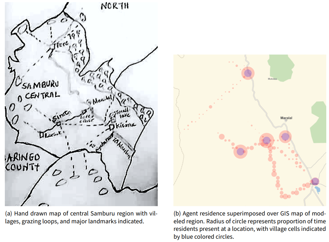
We chose to use path data from human sources residing in the region instead of heuristic decisions made by agents. Initial experiments with designing heuristics to drive agent movement were unable to replicate the observed behavior of people living in the region. As such, the use of available track data allows the model to best reflect the actual activities that humans in the region engage in. Future extensions to the movement model may use a hybrid approach in which track data obtained from residents are used to constrain computationally generated paths.
Geospatial data
Our model is driven by external data obtained from GIS sources for the central Samburu county region of Kenya. The region we have considered spans the latitude/longitude bounding box (0.91264, 1.24496) and (36.38761, 36.89965) as shown in Figure 2.
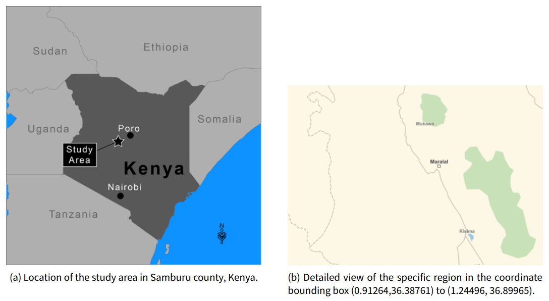
Within this region we have a set of village coordinates, permanent water feature coordinates, and known movement paths that herdsmen traverse. The region of interest is discretized into a cartesian grid of cells 1km-by-1km. Each cell is assigned a unique identifier used to merge GIS data sources. The latitude and longitude of the centroid of each cell is also stored. This is used to map between world cell coordinates and real world coordinates for sub-models defined on continuous latitude/longitude coordinates. For example, the agent movement model tracks the precise location of agents to allow for a fixed movement speed regardless of direction. An efficient bisection search algorithm is used to perform the mapping from latitude/longitude coordinates and grid cells.
We consider the following GIS data sources at the cell level: precipitation (cm); normalized difference vegetation index (NDVI); and foraging condition index (FCI). NDVI and FCI are unitless index values. Precipitation and NDVI are available to the model, but are not currently used in the governing equations at runtime. Precipitation is a driver for diseases in which waterborne vectors (mosquitos) are the primary infection source for RVF. Instead of using directly modeling the disease vectors as an emergent effect from precipitation observations (as in Gachohi et al. 2016 and Gachohi 2015), we use precipitation to precompute the coefficients for a harmonic function that drives infection (see Section 2.30).
Vegetation availability
One of the core concerns of the model is to capture vegetation availability for two purposes. First, vegetation availability is used to drive the health of grazing livestock. Second, relative vegetation availability between cells gives human agents the necessary input to calculate a preference that drives movement decisions. The current model uses foraging condition index (Matere et al. 2020; Stuth et al. 2005) as a proxy for vegetation availability. The ideal model would allow us to use some measurement of vegetation (e.g., NDVI or FCI) to estimate the vegetation mass present in a grid cell that is available to the livestock for nutritional input. This could then be connected directly to knowledge about animal physiology with regard to the amount of biomass necessary for livestock to maintain a specific level of health. Unfortunately, reasonable estimates of available vegetation mass components, quality and quantity are unavailable within the literature.
Instead, vegetation availability is calculated based on the following reasoning. Over the simulation epoch (2004-2015), we assume that the average climate conditions in the region are in fact average, and do not represent a long-term drought or high precipitation period. As such, the average conditions represent the conditions under which the livestock and residents of the region expect as a baseline for what constitutes average health. Instead of computing the absolute vegetation presence as a measure of mass or volume, we instead calculate the deviation from this average at each time step. For a grid cell \((i,j)\) at time \(t\), we calculate:
| \[ veg_{ij}(t) = \frac{FCI_{ij}(t)}{\mbox{avg}(FCI_{ij})}\] | \[(1)\] |
Agents
The human agents are the primary component of the model bridging submodels for animal health, movement, and vaccination decisions. Two classes of human agents are modeled: heads of household and herdsmen. This is intended to mimic the social structure present in the region of interest in which a senior member of a family is responsible for decision making with respect to the economic state of a family. A junior member of the family plays the role of herdsman, directly managing the herd of livestock owned by the family by making decisions regarding grazing and herd movement. The model currently associates a single herdsman to each head of household. The simulation supports households in which a head of household manages multiple herdsmen, but that mode is not currently used.
Each head of household and herdsman has a single village that they consider to be home. Heads of household are immobile agents and always reside within the village, and herdsmen prefer to remain at the village unless driven to move due to environmental factors where movement to a different region is preferable to meet the grazing needs of their herd. The event-based architecture of the model is easily extended to allow agents to initiate movement due to other factors, such as calendar date or decisions from heads of household. Such extensions will be explored in future revisions of the baseline model defined in this paper.
The head of household has state variables related to their recent vaccination decisions as well as their personal inclination for vaccination. These state variables are used in the decision model described below.
Herdsmen make the decision to move based on the vegetation state of their home village cell. Herdsmen start at these home cells and reside there until \(\mbox{veg}_{ij}(t) < \mbox{veg}_{thresh}\). At that point, the agent decides that the cell is no longer able to provide sufficient nutrition for their herd and movement is necessary.
Movement method
Initial versions of the model attempted to model movement purely computationally, but the movement tracks that were obtained did not exhibit realistic patterns as found in the literature (Liao 2018b, 2018a). Instead, we obtained maps of tracks drawn by people local to the area and digitized them as polygons (Figure 3). Each path starts at a known village and forms a closed cycle that ends at the same village. A path is defined as a set of cell waypoints where the agents traverse a straight line path between waypoints with a speed of 1km per day. Given that this results in movement at a finer granularity than the model cell size, herdsman location is modeled as direct latitude/longitude coordinates.
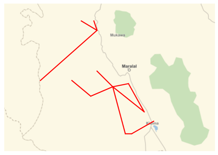
The rationale behind this movement model is based on information obtained from residents of the region. Herdsmen typically leave their village with their herds to seek regions known to have higher vegetation content, often around permanent (or frequent) water sources. When the foraging condition of their village drops below a pre-defined threshold, the agents pick a track that originates at their village at random, and traverse it in a cycle until they return to the home village. In the current model we do not allow agents to dwell at waypoints. A future revision of the model will include the ability to augment paths with information about dwell times at waypoints to represent expected behavior such as lingering at a known water feature or area rich in vegetation. This will be dependent on obtaining further information from residents of the region regarding movement habits.
Social network
Agents that communicate for decision-making purposes are connected in a social network. In this model the heads of household are the primary decision makers and are the only human agents in the network. Herdsmen communicate only with their corresponding head of household to receive vaccination commands. While herdsmen communicate with each other in the real world, those connections are currently not represented as they have no impact on any of the submodels. Future versions of the model may be extended in which herdsmen may communicate (e.g., long-distance phone calls to inform an agent about distant foraging conditions).
The social network is defined as a directed, weighted graph. For any agent \(i\) that has a social connection to a different agent \(j\), the weight matrix entry \(J_{ij}\) represents the weight of influence that agent \(j\) has on \(i\). The network is directed since the influence between individuals may not be symmetric. Any agents \(i\) and \(j\) that are not connected have weight \(J_{ij}=J_{ji}=0\). This weight matrix \(J\) is used within the decision model described in Section 2.19, specifically in the calculation of the agent incentive (Equation 2). We assume that the entries of \(J\) are in the interval \([-1,1]\).
Decision model
The Random Field Ising Model (RFIM) introduced by Bouchaud (2013) defines a spin system model for decisions in which individuals are influenced by the decisions of one or more others. Ising models are frequently used in economics to model the effect of network pressure on decision-making (Hokamp & Pickhardt 2010; Pellizzari & Rizzi 2014; Pickhardt & Seibold 2014). In our model we are concerned with the decision that each head of household makes regarding whether or not to vaccinate their animals against each of the diseases considered. The choice of an agent \(i\) is a boolean decision \(S_i \in \{-1,1\}\). The decision model to compute \(S_i\) integrates a number of factors both internal and external to an agent.
- The social influence \(J_{ij}\) between any two agents \(i\) and \(j\).
- Each agent \(i\) has their own internal preference \(f_i\), where \(f_i < 0\) indicates a preference towards \(S_i = -1\) and \(f_i > 0\) indicating a preference towards \(S_i = +1\).
- All agents have access to a public, time varying information source \(F(t)\) representing information from local authorities, public health officials, and so on. \(F(t)\) has a similar interpretation as \(f_i\).
For a single topic that an agent makes a decision about, we first calculate the perceived incentive for the \(i\)th agent:
| \[ U_i(t) = f_i + F(t) + \sum_{j \in \mathcal{V}_i} J_{ij} S_j(t-1)\] | \[(2)\] |
| \[\begin{aligned} P \left( S_i(t) = +1 | S_i(t-1) = -1; U_i \right) & = \frac{\mu}{1+e^{-\beta U_i}} \\ P \left( S_i(t) = -1 | S_i(t-1) = -1; U_i \right) & = 1 - \frac{\mu}{1+e^{-\beta U_i}} \\ P \left( S_i(t) = -1 | S_i(t-1) = +1; U_i \right) & = \frac{\mu}{1+e^{\beta U_i}} \\ P \left( S_i(t) = +1 | S_i(t-1) = +1; U_i \right) & = 1 - \frac{\mu}{1+e^{\beta U_i}}\end{aligned}\] | \[(3)\] |
At the start of the model each agent needs to be initialized with a decision value \(S_i(0)\). For each disease we define a probability \(P(S_i(0) = +1)\), and randomly assign initial decisions to each agent. This is defined on a per-disease basis to reflect differences in opinion within the population about the risk of infection and value of vaccination for each disease.
Selection of \(\beta\) and \(\mu\) parameters
The important parameters to consider in defining this probability are \(\mu\) and \(\beta\). The \(\mu\) parameter is interpreted by Bouchaud as modeling a one-step memory in which the most recent choice at time \(t-1\) has some bearing on the choice for time \(t\) when \(\mu \leq 1\). When \(\mu = 1\) the probability is memoryless. The \(\beta\) parameter is analogous to the temperature in a classical spin-glass system and is used to model noise. Bouchaud notes that when \(\beta \rightarrow 0\) incentives play no role and the decision reduces to a coin flip, and \(\beta \rightarrow \infty\) reduces to the opposite extreme in which the rule is deterministic where the choice corresponds to \(U_i\) exceeding some threshold value \(U_{th}\).
The sigmoidal function that appears in Equation 3 (i.e. logistic function) is defined over all reals, but the function is very close to 0 or 1 over all but a small region of its domain (approximately \([-4,4]\)). As a result, the range of \(\beta\) and \(U_i\) are important to consider. Examining Equation 2, the factor that accumulates the contribution of neighbors via \(J_{ij} S_j(t-1)\) is going to take on a value proportional to the number of agents in the neighborhood. Assuming that we restrict \(J_{ij}\), \(f_i\), and \(F(t)\) to the interval \([-1,1]\), then \(U_i \in [-(n+2),n+2]\). Thus we can select \(\beta \in \left[ 0, \frac{4}{n} \right]\) in order to explore the dynamics that emerge when \(P\) is not at the extreme values 0 or 1.
Disease model
The infectious disease component of the model uses a compartmented Susceptible, Infected, Recovered, Vaccinated (SIRV) model represented as a Markov transition system. The state transition system is illustrated in Figure 4.
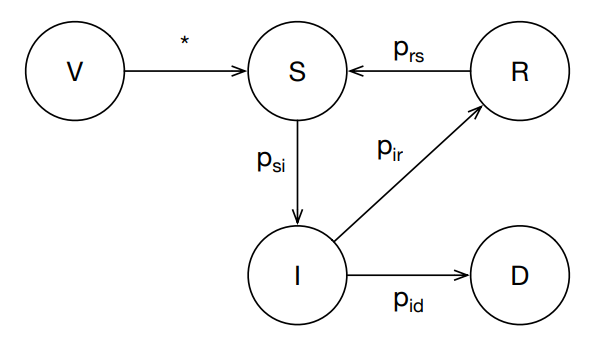
Each animal has a disease state for each modeled disease corresponding to one of the allowed compartments in the transition system. All animals are created in the susceptible (S) state. The death state (D) is not directly modeled as a state, but is included to represent the possible transition from the infected (I) state to death. For some diseases there is the possibility that an animal that has recovered (R) from infection may become susceptible in the future. Similarly, an animal that has been vaccinated (V) may become susceptible if the vaccine requires a periodic booster to keep it effective.
The transition edges represent the probability of an animal in a given state to transition to another state. An implicit self-transition is present for each state representing the probability that an animal in that state remains in it. For example, the probability that an infected animal remains infected is \(p_{II} = 1.0 - (p_{IR} + p_{ID})\). All transitions except \(p_{SI}\) are independent of the size of the herd that the animal resides within. The \(p_{SI}\) transition represents an infection event, which is proportional to the number of infected animals versus the herd size. Thus for a given animal, the probability of the \(S \rightarrow I\) is \(p_{SI} \frac{\#I}{N}\) where \(N\) is the herd size and \(\#I\) is the number of animals in the herd in the I state.
The transition probabilities are defined for a specific time scale. For the purposes of this model we have established a time scale of one day (Mariner et al. 2006). We obtained the transmission probabilities for RVF (Leedale et al. 2016) and CBPP (Mariner et al. 2006) from the veterinary medicine literature. These are shown in Table 1.
| Transition | RVF | CBPP |
|---|---|---|
| S \(\rightarrow\) I | 0.14 | 0.024 |
| I \(\rightarrow\) R | 0.0001 | 0.0045 |
| I \(\rightarrow\) D | 0.3 | 0.009 |
| R \(\rightarrow\) S | 0.0 | 0.0 |
The \(V \rightarrow S\) transition is modeled separately from the transition system since it has a time dependence. Due to the limited efficacy of the CBPP vaccine, when an animal is vaccinated at time \(t\), an event is scheduled reflecting depleted efficacy at some time \(t + \delta t\) where \(\delta t \sim N(\mu_d,\sigma_d)\) with \(\mu_d\) and \(\sigma_d\) being the mean and variance for vaccine effectiveness period for disease \(d\). Our model currently adopts a model of efficacy for the RVF vaccine in which animals require only one vaccination during their lifetime.
Disease transmission occurs between all animals colocated within a grid cell. Doing so allows diseases to transfer between herds while reflecting the knowledge that transmission requires proximity. This proximity factor would be lost using a simpler model in which we consider the entire population of animals regardless of location.
Environmental infections
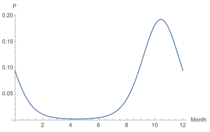
Infection is introduced into a population from environmental vectors for each disease. For diseases in which seasonal effects (e.g., precipitation driving mosquito populations) are the primary factor (i.e. RVF) we use a harmonic function fit to data obtained in a similar region (Lofgren et al. 2007). Specifically, we consider a model of the following form:
| \[Y(t)_i = \exp \left\{ \beta_{0,i} + \beta_{1,i} \cos(2 \pi \omega t) + \beta_{2,i} \sin (2 \pi \omega t) + \epsilon \right\}\] | \[(4)\] |
| Parameter | Coefficient | Std. Err. | \(z\) | \(P > |z|\) | 95% Conf. Interval | |
|---|---|---|---|---|---|---|
| \(\beta_{0,i}\) | -3.835099 | .5630832 | -6.81 | 0.000 | -4.938722 | -2.731476 |
| \(\beta_{1,i}\) | 1.487041 | .7208338 | 2.06 | 0.039 | 0.0742325 | 2.899849 |
| \(\beta_{2,i}\) | -1.610063 | .8473459 | -1.90 | 0.057 | -3.27083 | 0.050705 |
For diseases with a uniform probability of a random animal becoming infected we set a probability \(p_{*I}\) for some number of days \(\delta t\) (e.g., the probability of a single animal being infected in a single week). We then draw a sample every \(\delta t\) days and if an infection is determined to have occurred, we pick a random animal from the entire population to expose. All animals in the population are considered, which means that an exposure event may occur for an animal that is already infected or has immunity. This is intended to reflect that the prevalence of a disease in a population does not affect its ambient presence in the environment: the increase in spread due to its increase prevalence is taken care of via the animal-to-animal transmission dynamics discussed earlier. This assumption of a constant ambient disease source doesn’t reflect effects of an infected population on the environment (e.g., deposition onto surfaces and food sources), but is sufficient for our purposes in which the dominant mechanism of spread is inter-livestock transmission.
Livestock
Livestock are modeled at the individual animal level and herds managed by herdsmen (one herd per herdsman). Defining livestock agents by sex, age, reproductive capacity and nutritional health provides necessary realism to modeling herd dynamics. This aspect of realism in PastoralScape represents an advanced feature, relative to other ABMs (see Fust & Schlecht 2018; Bradhurst et al. 2016 for comparisons). The individual animals encapsulate health, reproductive, and disease state. A herd owned by a herdsman (and by proxy, a head of household) represents an economic unit. The herd also encapsulates reproduction dynamics and allows decisions made by individual human agents regarding movement and vaccination to be delegated to the correct set of individual animals.
A head of livestock has the following state variables:
- Health \(h \in [0,1]\) where 1 is optimal health, and 0 represents an animal that has died of malnutrition.
- Disease state. For each disease \(d\), an animal has a disease state from the set \(\{S, I, R, V\}\).
- Vaccination state. For each disease, the animal has a time of most recent vaccination \(t_{vacc}^d\). This is used to drive the transition \(V \rightarrow S\) for vaccines requiring periodic boosters.
An animal may die due to three factors: disease, malnutrition, and old age.
Aging
Age-related effects are modeled by defining a mean lifespan \(\mu_{age}\) and the variance \(\sigma_{age}\) of that expected lifespan. When an animal is created the lifespan is determined assuming that it survives disease and malnutrition. An event is created corresponding to this natural death event and scheduled upon animal creation. If an animal dies for some other reason, the agent is deactivated and this (and any other) event that occurs after its death is ignored.
Nutritional health
Nutritional health of the animal corresponds is represented by \(h\). When \(h = 0\), the animal is considered to have died of malnutrition. Nutritional health is updated for a whole herd at once with the assumption that available food is distributed uniformly amongst all members of the herd. The model has a parameter \(p_{foodneed}\) representing the number of units of food required by an individual animal in a single week. In the absence of a measure of vegetation mass, we instead calibrate the food requirement by grazing area required. For example, for a \(1\mbox{km}^2\) cell, if a single animal requires \(10\mbox{m}^2\) of grazing per day, then \(p_{foodneed} = 10^{-5}\). Thus for a timestep of \(\delta t\) days for a herd of size \(n\) with the provided parameter \(p_{foodneed}\), the required food is:
| \[food_{req} = p_{foodneed} * \delta t * n.\] | \[(5)\] |
We calculate the proportion of required units of food for a grid cell from the vegetation capacity (Equation 1).
When \(veg_{ij}(t) = 1.0\), the cell is guaranteed to have sufficient food to satisfy all of the needs of the animals present. When \(veg_{ij}(t) < 1.0\), the cell is partially barren and can only produce a fraction of the required food. Similarly, when it is greater than \(1.0\), the cell has more food than average available. For a \(1km^2\) cell, we then calculate:
| \[food_{avail} = \min \left(\frac{1000^2 * veg_{ij}(t)}{food_{req}}, 1.0\right)\] | \[(6)\] |
| \[r = \frac{food_{avail}}{food_{req}}\] | \[(7)\] |
Two rate parameters are defined \(h_{fed}\) and \(h_{starve}\). The \(h_{fed}\) parameter dictates the rate at which the health of the animal increases per day as it obtains food, while \(h_{starve}\) dictates the rate that it degrades per day when insufficient food is provided. These rates are separate to model a slower decline due to starvation versus a faster rate of recovery due to sufficient food. The health \(h\) of an animal is updated via:
| \[h = \min \left( 0.0, \max \left( 1.0, \mbox{ } h + h_{fed} * r * \delta t - h_{starve} * (1.0 - r) * \delta t \right) \right)\] | \[(8)\] |
Reproduction
Animal reproduction is modeled very simply. The lifecycle of a cow is split into four phases: immature, mature, pregnant, and nursing (Figure 6). An immature cow has not reached sexual maturity and cannot reproduce yet. A mature cow is able to reproduce if their health is above a threshold \(h_{reproduce}\). This health threshold captures the requirement that a cow must be sufficiently healthy to both maintain their own health as well as that of the developing offspring. A mature and healthy cow may become pregnant with some probability that is a function of the number of bulls co-located within a cell during a timestep. Finally, a pregnant cow that gives birth to a single offspring enters the nursing phase during which it cannot get pregnant again until it exits the nursing state after a fixed period of time and returns to the mature state. It is important to note that the nursing period modeled only reflects the nursing period during which a cow cannot become pregnant again. A cow that returns to the mature state after nursing may still nurse their offspring, but this “nursing and fertile” state is not currently explicitly modeled.
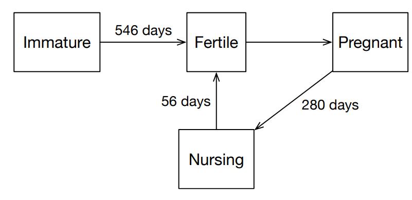
The state transition system for a head of cattle is represented by scheduled events. When a cow is born an event is scheduled to flag it as mature. When a cow becomes pregnant, an event is set at the end of the gestation period when it gives birth. Upon giving birth, the new animal is created and the cow enters the nursing state. An event is scheduled for the time at which the animal becomes fertile and can reproduce again. It is important to note that this transition does not correspond to the biological end of the nursing period, as cattle may continue nursing their offspring after they have become pregnant again. Instead we only model the period during nursing when a new pregnancy cannot occur.
The set of PastoralScape sub-models, described above, represent a complex set of interconnected systems. The modeling approach used captures realism of agents. This realism is reflected in modeling agents’ environments and social networks, their movements, nutritional health status of livestock, and informational and cognitive factors that affect human decision-making. The next section details the sequencing and initialization of the model.
Implementation
The model is implemented in Python 3 using an event-driven architecture. Our initial model used a single main time-stepping loop with a fixed timestep, but this proved inflexible for a number of reasons. First, different components of the model naturally map to different time scales: GIS data is updated at the start of each month; movement is defined in terms of distance travelled per day; disease progression and livestock health are modeled on a fortnight or weekly basis; vaccination decisions are made at specific calendar dates throughout the year. As such, we had two choices: run at the finest timescale such that each action to model falls on a timestep, or use an event driven model in which the progress of time is driven by the timing between events. The later proved to be simplest to implement and is most flexible for future model extensions, and has been adopted in other ABMs for similar reasons (Meyer 2015).
The core of the model is a driver that moves through an initialization phase and then an execution phase. The initialization phase entails creating all model objects (agents, world objects, disease objects, and so on) followed by the creation of all events that are known to occur over the span of the simulation - specifically, the week-granularity events for disease propagation and livestock health and the monthly events to update the world state from GIS data sources. The execution phase is then a simple loop in which the event queue (implemented as a min-heap, or priority queue) is checked to obtain the next event in time. An event is represented as a triple: the time for the event, the type of event, and the subject of the event.
Time is represented using Python date objects that allow a representation of calendar dates as well as date arithmetic (e.g., days between events; some date plus 2 weeks; etc.). Dates are serialized in the model output as days elapsed from the start of the simulation epoch. This overcomes issues with date representation in the output while retaining a straightforward mapping from day-of-simulation to calendar date given the calendar date of the simulation start.
Event types are a simple enumeration value. The model currently implements the following event types with corresponding event subject types.
GISUPDATE: A GIS update corresponds to a data input event in which static data obtained from sources external to the model are input as environmental sources. These may be real-world data measurements or outputs from external models (such as a climate or vegetation simulation). No subject object is necessary given that the model contains one and only one world object.MOVEMENT: A movement event represents a step in a path that an agent in motion is traversing. The subject of the movement event is the individual herdsman agent that is moving. The event is handled by the agent taking a single step along their movement path and checking whether or not they have returned to their home village. If they are not yet back home, the agent adds an event with themself as the subject to the event queue corresponding to the future time of their next movement step. AWORLDSTEPevent is also added to ensure that the disease and foraging models step forward as well.LIV_BIRTH: A birth event is created upon the start of pregnancy at a point in time in the future when the gestation period is over. The subject of this event is the pregnant cow, and when the event occurs the cow transitions into the nursing state and a new animal is created. The transition to nursing causes a future event to be scheduled for when the cow returns to fertility. During creation of the new animal the set of lifetime events (maturity, death by old age) are also scheduled.LIV_FERTILE: A fertility event occurs when an animal either matures from childhood or is already mature and is transitioning out of the nursing state. The subject of the event is the cow that is entering the fertile state.WORLDSTEP: A world-step event drives disease propagation and herd foraging activities. These activities progress by \(\delta t\) days representing the time since the last world-step event. The use of variable timestep sizes allows for the model to adapt to the finest timescale necessary at any given point in time. For example, while no agents are moving the model can proceed at a large step size (e.g., \(\delta t\) = 7 days). When agents move at a speed of 1km/day, it is necessary to step faster to avoid a case where an agent may pass through a cell without foraging and disease propagation occurring. This is critical since movement and the resulting colocation of herds from different villages is necessary for disease to propagate across the full agent set. No explicit subject is associated with the event since it applies to the single world object for the model.AGENTSTEP: Agent-step events correspond to regular, frequent decision making by human agents. In the current model heads of household do not make regular (e.g., daily or weekly) decisions so they ignore these events. Herdsmen use these events to assess the vegetation state of the cell in which they currently reside to determine if it is necessary to move. If such a decision is made, the herdsman creates a movement event and a worldstep event to ensure that after taking a step and potentially crossing into a new cell, the disease and foraging models step forward.VACCINATE: A vaccination event represents a time at which all heads of household make a decision about vaccinating their herd. This is typically modeled as a calendar date (e.g., Sept. 1st every year). This triggers the evaluation and update of the Random Field Ising Model state and calculation of a boolean vaccination decision for each disease present in the population.WEAROFF: A “wearoff” event is scheduled for vaccines that require periodic boosters (i.e. CBPP) due to the short duration of immunity provided by the vaccine. The subject of the event is the animal that will transition from vaccinated to susceptible, as well as the disease to consider. The time of the event is based on the mean and variance for the period of effectiveness for the disease relative to the time of vaccination.INFECTION: Infection events correspond to spontaneous transitions from susceptible to infected for some livestock. These are intended to capture environmental infections versus animal-animal transmission. Each disease is sampled with the appropriate environmental infection model (harmonic vs uniform) as described in Section 2.30.CULL_OLDAGE: An age-based culling event represents the animal subject of the event naturally dying of old age. These events are predetermined when an animal is created by sampling the distribution of lifespans for animals. Upon this event occuring, an animal is removed from all herds and set inactive. The inactive state allows any future events related to this animal that are already in the queue to be disregarded.
Events that are delegated to an agent set are handled in three phases. First, a pre-handler is called in order to perform bookkeeping prior to the set of agents handling the event. In the case of the decision model, this pre-handler shifts the most recent decisions simultaneously for all agents to the prior decision slot. This must occur before the core handler steps the decisions forward. A final post-handler is called after each agent in the set has handled the event. This currently performs no actions, but is present for potential future use with new event types.
Initialization
The model is initialized by creating a set of model objects corresponding to the input data and parameter set. The world grid and grid cells are created based on the discretization of the world into 1km-by-1km cells. A set of village cells are created at the coordinates specified in the input parameters. A set of heads of household are created and uniformly allocated amongst the villages. For each head of household a single herdsman is created and colocated with the head of household. The set of animals is created and allocated amongst the herdsmen uniformly. The distribution of animals is defined by the following parameters:
- \(p_{bull}\): To reflect the expected steady-state population, the sex distribution is determined by the fraction of animals that are bulls versus cows.
- \(min\_age\) and \(min\_remain\): Animals are created with a non-zero age. This age has some minimum value, and each animal must have some minimum time remaining alive from the start of the simulation epoch. Ages are uniformly distributed between those values given the lifespan distribution of animals.
- \(h_{start}\): All animals start with some initial health value. Currently all animals are created with the same initial health.
The initial population is created with some proportion in the vaccinated state for each disease. A per-disease proportion is specified in the input parameters. Those animals that are selected to be vaccinated are assumed to have been vaccinated in the most recent vaccination round prior to the start of the simulation based on the specified vaccination schedule. If the wearoff period of a vaccine from this date is calculated to fall before the start of the model, the corresponding animal is treated as unvaccinated.
With respect to the reproduction submodel, any cow beyond their age of maturity starts in a fertile state and can begin the reproductive process immediately. No animals are created in the pregnant state.
Once the herds and human agents have been created and all model objects created, the initial schedule of events is established by populating the model event queue. Using the specified default time step \(\delta t\), these initial events include:
- World and agent step events at a regular interval of \(\delta t\) days.
- GIS update events at the start of each calendar month.
- Vaccination dates at one or more calendar dates each year (e.g., September 5th).
- Environmental infection source sampling events at regular intervals of \(\delta t\) days.
- Old-age culling and animal maturation events for the initial animal population.
Experiments
A series of experiments are run to: i) test the speed of convergence and population split according to different \(\mu\) and \(\beta\) parameter values, ii) the number of livestock deaths (all causes) as \(\mu\) changes, and iii) the distribution of RVF and CBPP deaths seasonally. These experiments demonstrate the utility of the PastoralScape model. The flexibility and realism of allowing for rationality and memory capacities to differ over time and between individuals captures cognitive dynamics evident among the global poor (Iles et al. 2021).
Sensitivity of RFIM to \(\beta\) and \(\mu\) selection
Understanding the interplay between the parameters for the RFIM component of the overall model is important in parameter selection. We consider configuration of the RFIM component as defined in Table 3 in isolation of the other model components.
| Parameter | Value |
|---|---|
| Population size | \(n = 60\) |
| Social network | \(J_{ij} ~ U[-0.2, 0.8]\) |
| Internal preference | \(f_i = 0\) |
| External information | \(F(t)\) varied over \([-8,8]\) by steps of \(0.2\) |
| Initial decision state | \(P(S_i(0) = +1) = 0.4\) ; \(P(S_i(0) = -1) = 0.6\) |
| Timesteps | 100 |
| \(\beta\) | \(\{ 0.01, 0.1, 0.3 \}\) |
| \(\mu\) | \(\{ 0.05, 0.3, 0.75 \}\) |
The population of \(n\) individuals is created in a fully connected social network with weight of influence ranging from \(-0.2\) to \(0.8\). This choice of interval causes the majority of connections to be positively reinforcing, and the few that are negatively reinforcing do so with relatively small weight. Given that both \(f_i\) and \(F(t)\) are similar in the definition of \(U_i\), we fix \(f_i\) at 0 for all individuals and fix \(F(t)\) at a constant during a run. For a given selection of \(\beta\) and \(\mu\) we vary \(F(t)\) to see how the evolution of the decision state across the population varies. We initialize the decision state, \(S_i(0)\), for all individuals in the population to have a slight bias in one direction. For each parameter combination, we perform an ensemble of 25 runs and calculate the average \(|\{S=+1\}| - |\{S=-1\}|\). When all agents are in agreement, this value takes on \(\pm n\) (color axis of Figure 7 ranges from -60 to +60), and when the population is split in half it is zero. Otherwise it gives a measure of the degree of imbalance with which the population is split.
The results of these experiments are shown in Figure 7. We can see a few interesting features emerge. First, the lowest \(\beta\) value agrees with the interpretation given by Bouchaud - when \(\beta \rightarrow 0\) the system is noise-dominated regardless of the memory that agents have of past decisions. As \(\beta\) increases, we see that the system reaches a stable state much more quickly since the lack of noise prevents this convergence from being disrupted. Second, as \(\mu\) is varied, we see the effect of the last-decision memory. For example, when \(\beta=0.1\) we see for the lowest value of \(\mu\) the system takes longer to stabilize, while for the largest \(\mu\) value it stabilizes within only a few iterations. This appears to indicate that when the system is memoryless the state of the agents relaxes to agreement based on the current state of the population, while the presence of a memory causes some agents to effectively resist changing to the lower energy state from their previous decision.
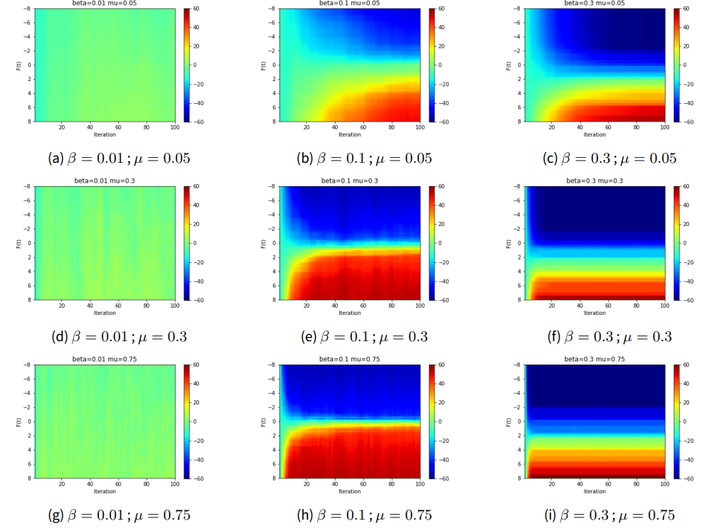
Finally, we are able to see that the public information \(F(t)\) is able to influence the collective opinion with a transition that depends on the parameter selection. For example, with the moderate \(\beta\) and \(\mu\) values we see a rapid shift where the population collectively takes on one value of \(S\) and after a slight change in \(F\) collectively changes their mind. When noise dominates for low \(\beta\), the value of \(F(t)\) has no effect. Interestingly, when \(\beta\) increases, \(\mu\) does not appear to have any effect on the sharpness of the transition and the effect of \(F(t)\) is much smoother.
We use these results to calibrate our choice of parameters for the RFIM in integration with the other sub-models. Specifically, given a desired model period of 11 years with one or two vaccination decisions per year, we expect \(\mu\) around 0.3 to be ideal - it allows the system to converge to a consensus state relatively quickly while allowing the agents to retain some memory of past choices. Similarly, \(\beta\) should be kept near \(0.1\).
Effect of \(\mu\) in overall model
The computational experiments presented span a time period from 2004 through 2015. Transition parameters for the Markov SIRV model are shown in Table 1. The timestep is \(\delta t = 7\) days. RVF infection introduction is governed by a harmonic function fit to precipitation data. The parameters for this function are shown in Table 2. The CBPP infection rate is \(p_{cbpp} = 0.025\) (the probability that a single animal in the population will be infected over \(\delta t\) days). The initial population of households is \(n=150\) distributed uniformly between all five villages, with a single head of household agent and herdsman per household. The initial livestock count is \(n=1500\) uniformly distributed amongst the herdsmen. The initial livestock population is composed of \(30\%\) bulls and \(70\%\) cows. Livestock are created with ages uniformly distributed between 1.5 and 9 years old, with no animals pregnant initially. The \(f_i\) parameter of the RFIM for each head of household is set to 0.1, with a \(60\%\) probability of having \(S_0=+1\) as their starting decision state.
Using the results from the isolated RFIM study regarding the model response to \(\beta\) and \(\mu\) variation, we perform a set of studies with \(\beta = 0.1\) and vary \(\mu\) from 0 through 1. This allows us to explore the short-term memory effect modeled by \(\mu\) on the overall outcome of herds over the 11 year period. As we see in Section 4.1, the memory parameter appears to play a role in the population reaching consensus for some fixed public information \(F(t)\). When consensus is reached, the agents either all choose to vaccinate or abstain. This occurs rapidly within only a few decision making steps for high values of \(\mu\), but for lower values consensus either takes longer to emerge or fails to emerge at all. The choice of \(F(t)=1.0\) falls within the region of the parameter space where we see the phase transition from universal vaccine abstinence to universal acceptance. An ensemble of 100 runs was performed for each choice of \(\mu\) varying the random number generator seed for each run. The results are shown in Figure 8.
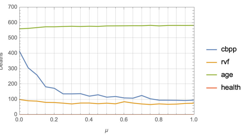
The results show that, as expected, the memory effect does make a difference. When no memory of the most recent decision is considered, a high death count occurs, especially for CBPP. As \(\mu\) increases and this short term memory plays a stronger role in the vaccination decision, we see the number of deaths flatten out after \(\mu \approx 0.35\).
Effect of annual vaccine timing
The seasonal variation in disease prevalence for Rift Valley Fever implies that the date of vaccination may have an impact on the overall resilience of herds to disease, especially with respect to animals born in the time period since the last vaccination event. In this study we fix all parameters other than the date of vaccination. We perform an ensemble of 1,000 runs for vaccinations timed at the start of each month (for a total of 12,000 runs to cover the entire year). The results are shown in Figure 9.
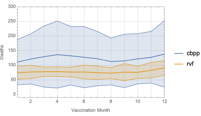
We observe that CBPP has a much higher variability than RVF largely due to the selection of spontaneous environmental infections as well as declining (or less durable) vaccinal immunity. RVF exhibits less variability across runs due to the modeled lifetime effectiveness of the vaccine which results in a lower number of susceptible individuals at any given time. We do observe an increase in RVF deaths when the vaccination occurs later in the year, as that corresponds to the higher probability of infection driven by the harmonic function shown in Figure 5. This is due to animals born since the previous vaccination being more likely to be infected during the period of the year in which mosquitos are more prevalent.
Parameter selection discussion
The most significant gap in this work requiring further data collection is the selection of parameters for disease prevalence and the relationship between vegetation measures (FCI or NDVI) to available food for livestock. In both cases the literature is limited within this region. We have found, for example, that the choice of environmental infection probability for both diseases has a significant impact on mortality - especially for CBPP where vaccination is not lifetime. Similarly, the choice of parameters to calculate the necessary food per head of livestock is based on information from western farming sources. Very limited information is available for animals in the Kenya region that are managed very differently than those present in dedicated livestock farms. Finally, while we used available data from the geographically nearby Baringo district, further work is necessary to determine what difference is to be expected in the Samburu region. In particular, the Samburu region contains mountainous areas which may impact precipitation patterns differently than those in Baringo.
Conclusions
This paper presents a model for human decision making for disease vaccination via a coupled human and natural system (CHNS). The PastoralScape CHNS model uses historical environmental data to drive livestock disease transmission, livestock health and reproduction. The development of the PastoralScape model in this paper, first introduced by Iles et al. (2020), details the behavioral utility of the logit transformed RFIM in capturing human decision making. The interaction between the values of \(\mu\), \(\beta\) and fixed values of RFIM parameters provides one indication of the potential of this human decision making paradigm to add value to ABM modeling of human agents. Although convergence of opinion is reach across various \(\mu\) and \(\beta\) values, the speed of this convergence differs. As such, we demonstrate that depending on the frequency of modeled human decisions, the rate of convergence may be tailored to fit.
In the context of evaluating the utility of the logit transformed RFIM in modeling one-time (i.e. once-for-life vaccines) and annual decisions (i.e. annual booster vaccines), the frequency of annual decisions shows greater sensitivity to changes in \(\mu\) and \(\beta\). Applications of the logit transformed RFIM to decision contexts with greater frequency of decisions is needed.
Although the selection of \(\mu\) and \(\beta\) in each run is uniform and constant across all decision makers in this paper, this need not be the case. A likely more realistic scenario is where the \(\mu\) and \(\beta\) parameters are allowed to vary across decisions makers. In the context of modeling absolute poor livestock owners, variables affecting changes in cognition parameters (\(\mu\) and \(\beta\)) include: rainfall and perceptions of financial well-being (Iles et al. 2021; Mani et al. 2013). In so doing, greater levels of coupling between human and natural systems may be achieved. The use of the logit transformed RFIM with dynamic cognition parameters across decision makers would represent a significant advance in modeling human decision making in ABM enabled coupled human and natural systems.
Acknowledgements
The authors would like to thank Timothy Lesimalele for collecting path data from residents of the region of study and providing the hand-drawn maps used in this work. John Gachohi and Samson Leta also provided input on the design of the disease models in the context of the region of study. Support for this research was provided to R.I by the New Faculty Seed Funding grant 2018, Washington State University. This work was performed by M.S. under the auspices of the U.S. Department of Energy by Lawrence Livermore National Laboratory under Contract DE-AC52-07NA27344.References
AKTIPIS, A., de Aguiar, R., Flaherty, A., Iyer, P., Sonkoi, D., & Cronk, L. (2016). Cooperation in an uncertain world: For the Maasai of East Africa, need-Based transfers outperform account-keeping in volatile environments. Human Ecology, 44, 353–364. [doi:10.1007/s10745-016-9823-z]
AKTIPIS, C. A., Cronk, L., & de Aguiar, R. (2011). Risk-Pooling and herd survival: An agent-Based model of a maasai gift-Giving system. Human Ecology, 39, 131–140. [doi:10.1007/s10745-010-9364-9]
AN, L. (2012). Modeling human decisions in coupled human and natural systems: Review of agent-based models. Ecological Modelling, 229, 25–36. [doi:10.1016/j.ecolmodel.2011.07.010]
ARGENT, J., Augsburg, B., & Rasul, I. (2014). Livestock asset transfers with and without training: Evidence from Rwanda. Journal of Economic Behavior & Organization, 108, 19–39. [doi:10.1016/j.jebo.2014.07.008]
BANERJEE, A., Duflo, E., Goldberg, N., Karlan, D., Osei, R., Parienté, W., Shapiro, J., Thuysbaert, B., & Udry, C. (2015). A multifaceted program causes lasting progress for the very poor: Evidence from six countries. Science, 348(6236), 1260799–1260799. [doi:10.1126/science.1260799]
BOUCHAUD, J. P. (2013). Crises and collective socio-Economic phenomena: Simple models and challenges. Journal of Statistical Physics, 151, 567–606. [doi:10.1007/s10955-012-0687-3]
BRADHURST, R. A., Roche, S. E., East, I. J., Kwan, P., & Garner, M. G. (2016). Improving the computational efficiency of an agent-based spatiotemporal model of livestock disease spread and control. Environmental Modelling & Software, 77, 1–12. [doi:10.1016/j.envsoft.2015.11.015]
COHEN, J. M., Sauer, E. L., Santiago, O., Spencer, S., & Rohr, J. R. (2020). Divergent impacts of warming weather on wildlife disease risk across climates. Science, 370(6519). [doi:10.1126/science.abb1702]
FUST, P., & Schlecht, E. (2018). Integrating spatio-temporal variation in resource availability and herbivore movements into rangeland management: RaMDry - An agent-based model on livestock feeding ecology in a dynamic, heterogeneous, semi-arid environment. Ecological Modelling, 369, 13–41. [doi:10.1016/j.ecolmodel.2017.10.017]
GACHOHI, J. M. (2015). A simulation model for Rift Valley fever transmission. Thesis. Nairobi, Kenya: University of Nairobi. Accessible at: http://erepository.uonbi.ac.ke/bitstream/handle/11295/95310.
GACHOHI, J. M., Kariuki Njenga, M., Kitala, P., & Bett, B. (2016). Modeling vaccination strategies against Rift Valley Fever in Livestock in Kenya. PlOS Neglected Tropical Diseases, 11(1), e0005316. [doi:10.1371/journal.pntd.0005316]
GALVANI, A. P., Bauch, C. T., Anand, M., Singer, B. H., & Levin, S. A. (2016). Human-environment interactions in population and ecosystem health. Proceedings of the National Academy of Sciences, 113(51), 14502–14506. [doi:10.1073/pnas.1618138113]
HAILEGIORGIS, A., & Crooks, A. (2012). Agent-based modeling for Humanitarian Issues: Disease and Refugee Camps. Proceedings of the The Computational Social Science Society of America Conference, Santa Fe, NM. [doi:10.1109/wsc.2013.6721551]
HAILEGIORGIS, A., Crooks, A., & Cioffi-Revilla, C. (2018). An agent-Based model of rural households’ Adaptation to climate change. Journal of Artificial Societies and Social Simulation, 21(4), 4: https://www.jasss.org/21/4/4.html. [doi:10.18564/jasss.3812]
HAILEGIORGIS, A., Kennedy, W. G., Rouleau, M., Bassett, J. K., Coletti, M., Balan, G. C., & Gulden, T. (2010). An agent based model of climate change and conflict among pastoralists in east Africa. 2010 International Congress on Environmental Modelling and Software Modelling for Environment’s Sake.
HAO, Y., Armbruster, D., Cronk, L., & Aktipis, C. A. (2015). Need-based transfers on a network: A model of risk-pooling in ecologically volatile environments. Evolution and Human Behavior, 36, 265–273. [doi:10.1016/j.evolhumbehav.2014.12.003]
HEDGE, M., & Leith, K. (2016). Goat herder needs assessment, Odisha, India. Tech Report. D-Lab, MIT.
HERRERO, M., Addison, J., Bedelian, C., Carabine, E., Havlı́k, P., Henderson, B., van de Steeg, J., & Thornton, P. K. (2016). Climate change and pastoralism: Impacts, consequences and adaptation. Revue Scientifique et Technique - Office International Des Epizooties, 35(2), 417–433. [doi:10.20506/rst.35.2.2533]
HOKAMP, S., & Pickhardt, M. (2010). Income tax evasion in a society of heterogeneous agents: Evidence from an agent-based model. International Economic Journal, 24(4), 541–553. [doi:10.1080/10168737.2010.525994]
ILES, R. A., Sottile, M. J., Amram, O., Lofgren, E., & McConnel, C. S. (2020). Variable cognition in ABM decision-Making: An application to livestock vaccine choice. Frontiers in Veterinary Science, 7, 788. [doi:10.3389/fvets.2020.564290]
ILES, R. A., Surve, A., Kagundu, S., & Gatumu, H. (2021). The role of short-term changes in cognitive capacity on economic expenditure among Kenyan agro-pastoralists. PLoS ONE, 16(3), e0247008. [doi:10.1371/journal.pone.0247008]
KENNEDY, W. G., & Bassett, J. K. (2011). Implementing a "fast and frugal" cognitive model within a computational social simulation. Proceedings of the Second Annual Conference of the Computational Social Science Society of America, Santa Fe, NM.
KENNEDY, W. G., Cotla, C. R., Gulden, T., Coletti, M., & Cioffi-Revilla, C. (2014). 'Towards validating a model of households and societies in East Africa.' In S. H. Chen, I. Terano, H. Yamamoto, & C. C. Tai (Eds.), Advances in Computational Social Science: The Fourth World Congress (Vol. 20, pp. 315–328). Berlin, Heidelberg: Springer. [doi:10.1007/978-4-431-54847-8_20]
KENNEDY, W. G., Gulden, T., Rouleau, M., Hailegiorgis, A., Bassett, J. K., Coletti, M., Balan, G. C., & Cioffi-Revilla, C. (2010). MASON HerderLand: Modeling origins of conflict in East Africa.
KENNEDY, W. G., Hailegiorgis, A., Rouleau, M., Bassett, J. K., Coletti, M., Balan, G. C., & Gulden, T. (2010). An Agent-Based Model of Conflict in East Africa And the Effect of Watering Holes. Proceedings of the 19th Conference on Behavior Representation in Modeling and Simulation, Charleston, SC.
KRAMER, D. B., Hartter, J., Boag, A. E., Jain, M., Stevens, K., Nicholas, K. A., McConnell, W. J., & Liu, J. (2017). Top 40 questions in coupled human and natural systems (CHANS) research. Ecology and Society, 22(2). [doi:10.5751/es-09429-220244]
LEEDALE, J., Jones, A., Caminade, C., & Morse, A. (2016). A dynamic, climate-driven model of Rift Valley fever. Geospatial Health, 11(1), 394. [doi:10.4081/gh.2016.394]
LIAO, C. (2018a). Modeling herding decision making in the extensive grazing system in Southern Ethiopia. Annals of the American Association of Geographers, 108(1), 260–276. [doi:10.1080/24694452.2017.1328306]
LIAO, C. (2018b). Quantifying multi-scale pastoral mobility: Developing a metrics system and using GPS-Tracking data for evaluation. Journal of Arid Environments, 153, 88–97. [doi:10.1016/j.jaridenv.2017.12.012]
LIU, J., Dietz, T., Carpenter, S. R., Alberti, M., Folke, C., Moran, E., Pell, A. N., Deadman, P., Kratz, T., Lubchenco, J., Ostrom, E., Ouyang, Z., Provencher, W., Redman, C. L., Schneider, S. H., & Taylor, W. W. (2007). Complexity of coupled human and natural systems. Science, 317(5844), 1513–1516. [doi:10.1126/science.1144004]
LOFGREN, E., Fefferman, N., Doshi, M., & Naumova, E. N. (2007). 'Assessing seasonal variation in multisource surveillance data: Annual harmonic regression.' In D. Zeng, I. Gotham, K. Komatsu, C. Lynch, M. Thurmond, D. Madigan, B. Lober, J. Kvach, & H. Chen (Eds.), Intelligence and Security Informatics: Biosurveillance (pp. 114–123). Berlin, Heidelberg: Springer. [doi:10.1007/978-3-540-72608-1_11]
MANI, A., Mullainathan, S., Shafir, E., & Zhao, J. (2013). Poverty impedes cognitive function. Science, 341(6149), 976–980. [doi:10.1126/science.1238041]
MARINER, J. C., McDermott, J., Heesterbeek, J. A. P., Thomson, G., & Martin, S. W. (2006). A model of contagious bovine pleuropneumonia transmission dynamics in East Africa. Preventive Veterinary Medicine, 73(1), 55–74. [doi:10.1016/j.prevetmed.2005.09.001]
MARSH, T. L., Yoder, J., Deboch, T., McElwain, T. F., & Palmer, G. H. (2016). Livestock vaccinations translate into increased human capital and school attendance by girls. Science Advances, 2(12), e1601410. [doi:10.1126/sciadv.1601410]
MATERE, J., Simpkin, P., Angerer, J., Olesambu, E., Ramasamy, S., & Fasina, F. (2020). Predictive livestock early warning system (PLEWS): Monitoring forage condition and implications for animal production in Kenya. Weather and Climate Extremes, 27, 100209. [doi:10.1016/j.wace.2019.100209]
MCDERMOTT, J. J., Staal, S. J., Freeman, H. A., Herrero, M., & van de Steeg, J. (2010). Sustaining intensification of smallholder livestock systems in the tropics. Livestock Science, 130(1–3), 95–109. [doi:10.1016/j.livsci.2010.02.014]
MEYER, R. (2015). 'Event-Driven multi-agent simulation.' In F. Grimaldo & E. Norling (Eds.), Multi-Agent-Based Simulation XV (pp. 3–16). Berlin, Heidelberg: Springer International Publishing. [doi:10.1007/978-3-319-14627-0_1]
PELLIZZARI, P., & Rizzi, D. (2014). Citizenship and power in an agent-basedmodel of tax compliance with public expenditure. Journal of Economic Psychology, 40, 35–48. [doi:10.1016/j.joep.2012.12.006]
PICKHARDT, M., & Seibold, G. (2014). Income tax evasion dynamics: Evidence from an agent-based econophysics model. Journal of Economic Psychology, 40, 147–160. [doi:10.1016/j.joep.2013.01.011]
SCHLÜTER, M., McAllister, R. R. J., Arlinghaus, R., Bunnefeld, N., Eisenack, K., Hölker, F., Milner-Gulland, E. J., Müller, B., Nicholson, E., Quaas, M., & Stöven, M. (2012). New horizons for managing the environment: A review of coupled social-ecological systems modeling. Natural Resource Modeling, 25(1), 219–272. [doi:10.1111/j.1939-7445.2011.00108.x]
SKOGGARD, I., & Kennedy, W. (2013). An interdisciplinary approach to agent-Based modeling of conflict in Eastern Africa. Practicing Anthropology, 35(1), 14–18. [doi:10.17730/praa.35.1.26866282874725k4]
STUTH, J. W., Angerer, J., Kaitho, R., Jama, A., & Marambii, R. (2005). 'Livestock early warning system for africa rangelands.' In V. K. Boken, A. P. Cracknell, & R. L. Heathcote (Eds.), Monitoring and Predicting Agricultural Drought: A Global Study (pp. 283–296). Oxford, MA: Oxford University Press. [doi:10.1093/oso/9780195162349.003.0032]
THORNTON, P. K., Kruska, R. L., Henninger, N., Kristjanson, P. M., Reid, R. S., & Robinson, T. P. (2003). Locating poor livestock keepers at the global level for research and development targeting. Land Use Policy, 20(4), 311–322. [doi:10.1016/s0264-8377(03)00034-6]