
Introduction
In societies whose livelihoods rely on subsistence agriculture, the impact of climate change can have significant consequences for their survival. Climate change can place unprecedented stress on rural communities, as it will alter their resource base without giving them sufficient time for adaptation (Admasu et al. 2010; Gebresenbet & Kefale 2012; Oba 2001; Solomon 2007; Thornton et al. 2009). While rural systems have developed various adaptive strategies over many generations in order to survive, the alteration of any resources can significantly affect even highly regarded and accepted customs, and may lead to the displacement of populations along with other severe humanitarian consequences (Kniveton et al. 2011).
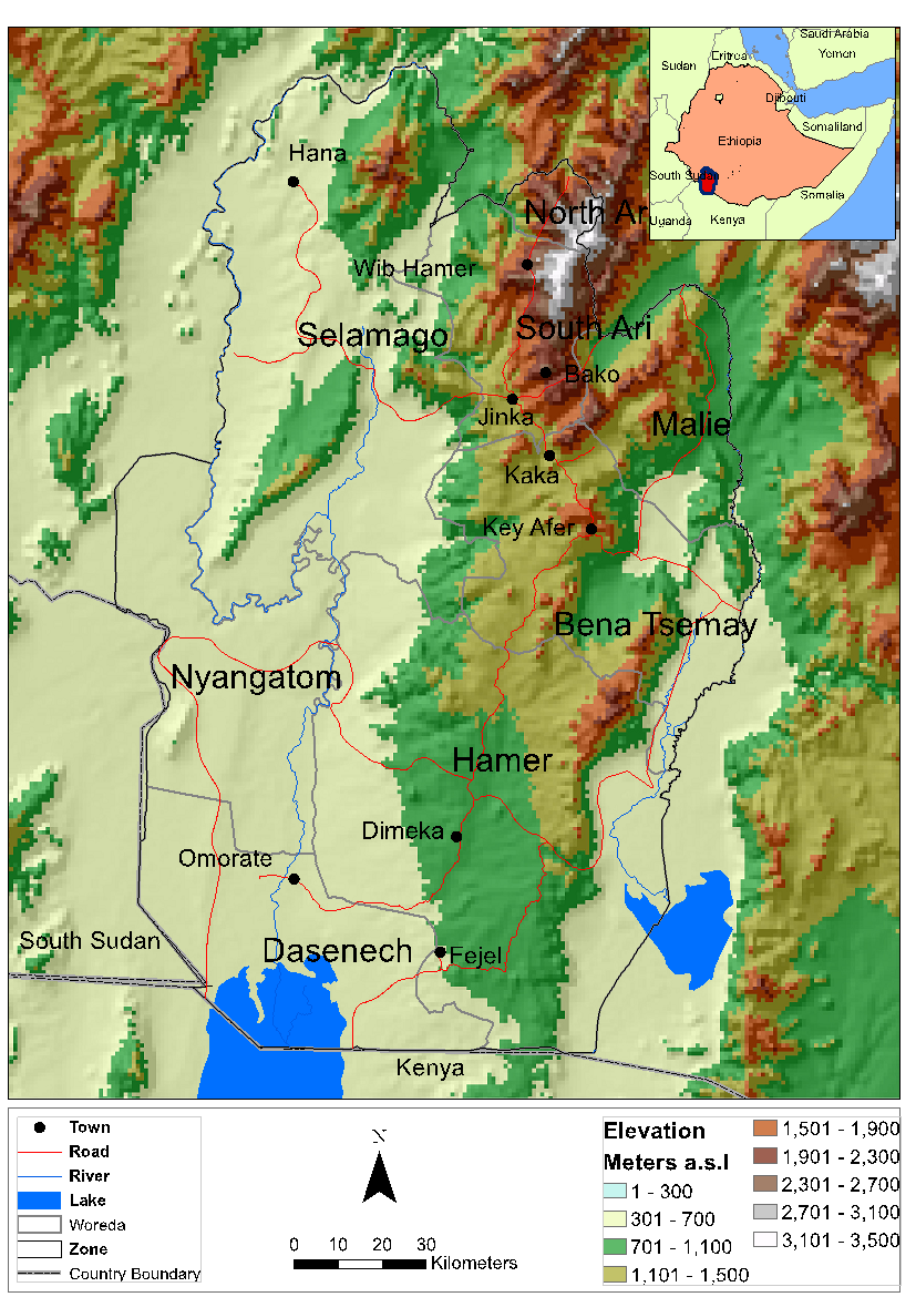
In this paper we focus on the South Omo Zone of Ethiopia, a region where climate change is expected to play a significant role in shaping the future socio-ecological setting of the region. The South Omo Zone covers an area of 2.3 million hectares and is located in the southern part of Ethiopia, bordering Kenya to the south and South Sudan to the southwest, as shown in Figure 1. It has a total population of over half a million people (570,000 inhabitants in 125,000 households) living in a traditional system of subsistence agriculture dominated by pastoral systems (CSA 2012). Historically, communities in this area have managed resources and their livelihoods in the face of challenging climatic conditions for many generations by applying different adaptation mechanisms, such as increasing herd size, diversifying herds or crops, or migrating (see Admasu et al. 2010; Gebresenbet & Kefale 2012). While there is significant uncertainty concerning the magnitude and direction of changes in rainfall under future climate change scenarios (Funk et al. 2008), the South Omo Zone provides an appropriate case-study for investigating rural household adaptation to climate variability and associated land use behaviors. Specifically, we address the following research questions, among others: Under which climate change conditions are households pushed beyond the limits of survival? How do various mixes of herding and farming affect household well-being under climate change conditions? What role do factors such as households’ ability to accurately predict weather events have on livelihoods and adaptation to climate change? In the remainder of this paper, we first provide some background pertaining to climate change adaptation and agent-based modeling (Section 2) which sets the scene for our model. Section 3 introduces in detail our study area and provides a detailed description of the OMOLAND-CA model, while in Section 4 we present results from the model under three different scenarios in order to address our research questions. Finally, in Section 5, we discuss policy implications of this study and identify areas of further research.
Background: Climate Change Adaptation and Agent-Based Models
Climate change adaptation
Adaptation to climate change, which includes adjustments in behavior or economics, can greatly reduce vulnerability to it by making rural communities more proactive to climate change and variability in weather. Adaptation can moderate potential damages and help rural communities cope with adverse consequences (McCarthy et al. 2001; Smith et al. 2011). Several adaptive measures have been discussed in previous research, including diversifying crops and varieties, changing planting dates, rotating crops, intensifying use of irrigation, expanding farm lands, implementing different soil conservation mechanisms, and diversifying household income sources (see, for example, Cooper et al. 2008; Deressa et al. 2009; Mendelsohn & Dinar 1999; Osbahr et al. 2008. Kniveton et al. (2011) also suggested that seasonal migration of people could be considered an adaptive mechanism, as seen in Burkina Faso. In the context of pastoral rural communities, Agrawal and Perrin (2009) suggested that basic adaptation strategies involve functions that share risks through mobility, storage, diversification, common pooling, and exchange of resources. A similar observation was also made by Morton et al. (2006) based on a review of studies on coping strategies of pastoralists during recent droughts and long-term adaptations in Northern Kenya and Southern Ethiopia. Morton et al. (2006) suggest that the most common adaptation strategies pastoralists use are increasing mobility, increasing herd size, diversifying herd composition, diversifying livelihoods, and sharing resources. Thornton et al. (2009) also suggested that farming, herd diversification, and increase in off-farm activities are the most common pastoralist adaptations. In addition, Adger et al. (2009) observed that use of local-based knowledge of resource systems and social networks to share risks also plays an important role in adaptation. Finally, open-access resources, such as wild foods, is another core adaptive mechanism (Eriksen et al. 2005; Mortimore & Adams 2001).
Although adaptation to climate change plays a significant role in rural systems, modeling adaptation is extremely complex due to (a) heterogeneity of rural households and (b) locational and contextual specificity of mechanisms by which rural communities respond to climate change and variability (Bryan et al. 2009; Morton 2007). Several studies have examined the factors that influence the capacity of rural communities to adapt and their priority for adaptation measures (see for example, Brooks et al. 2005; Smit et al. 2000; Smit & Skinner 2002; Yohe & Tol 2002). These studies emphasize the importance of natural resources and socioeconomic determinants—such as wealth, technology, information, skills, infrastructure, institutions, and equity—in shaping the adaptive behavior and the mechanism by which rural communities respond to climate variability. However, the role of cognition in adaptation to climate change has so far been largely neglected (Grothmann & Patt 2005; Kniveton et al. 2011). Smith et al. (2011) suggest that adaptation strategies depend not only on present households' characteristics and the surrounding biophysical environment, but also on previous experience and the networks to which households belong. Grothmann & Patt (2005) also argue that people's beliefs about risks, chances, and adaptation drive much of the process of adaptation to climate change. Individuals’ perception of climate-induced events, the timing of their responses, and their subsequent ability to manage, adapt to, or escape from the impact of these events determines the type of adaptation strategy used.
Agent-based climate change models
Agent-Based Modeling (ABM) is a natural way of representing socio-cognitive behavior of individuals and simulating complex interactions between individuals and their environment (Berger & Troost 2014; Cioffi-Revilla 2016; Geard et al. 2013). It provides a viable scientific approach for representing human decision-making processes (Balke & Gilbert 2014) and complex interactions between humans and their environments (both natural and artificial) at different spatial and temporal scales (Crooks & Heppenstall 2012). It has been argued that agent-based models are particularly useful for developing an understanding of the complex adaptive system under investigation, where assumptions about processes and interactions can be explored through simulation (Bert et al. 2015; Epstein 2008; Kelly et al. 2013; Lee et al. 2015). Moreover, it is also possible to use such models as computational laboratories for exploring interesting scenarios that focus on the local people’s adaptive responses to different socioeconomic factors and the underlying effects on their ecosystem (Crooks & Heppenstall 2012). Accordingly, several agent-based models have been developed to examine interactions between rural households and their environments, including assessing the consequences of household decisions on land-use and land-cover change (e.g., Bert et al. 2015; Deadman, et al. 2004; Liu et al. 2007; Etienne et al. 2003; Rindfuss et al. 2008; Saqalli et al. 2011); households’ migration behavior (e.g., Cioffi-Revilla et al. 2015; Entwisle et al. 2008; Kniveton et al. 2008; Smith et al. 2011); vulnerability to climatic factors (e.g., Acosta-Michlik & Espaldon 2008; Bharwani et al. 2005); adaptation to climate variability (e.g., Bommel et al. 2014; Cioffi-Revilla et al. 2010, 2015; Hailegiorgis et al. 2010); climate risk perception in land markets (e.g., Filatova et al. 2011; Putra et al. 2015); and diversification and adoption of new technologies (e.g., Berger 2001; Kaufmann et al. 2009).
Although previous models provide many insights on the impact of human actions on the environment and vice versa, they either exclude the representation of socio-cognitive behavior of households altogether or they greatly simplify the adaptive behavior and responses of households to climate change. In this paper, we present a spatiality explicit agent-based model of climate adaptation, namely the OMOLAND-CA (OMOLAND Climate Change Adaptation) model, which explicitly represents the socio-cognitive behavior of rural households towards climate change using the framework of the Model of Private Proactive Adaptation to Climate Change (MPPACC) proposed by Grothmann and Patt (2005). OMOLAND-CA is designed to explore interactions and decision-making among heterogeneous actors in rural systems, especially in rural households whose livelihood is closely coupled with climate and the biophysical environment. The model also enables exploration of climate variability impacts on actors and their biophysical environment; i.e., how feedback from the environment influences decision-making at different spatio-temporal scales.
Methodology
Setting, site, situation
The South Omo Zone is an area of some of 2.1 million hectares located in the southern part of Ethiopia. It borders with Kenya in the south and South Sudan in the southwest as shown in Figure 2. The topography of the Zone shows distinct gradient along a northeast-southwest direction. At the northeast of the zone, the elevation ranges between 2500-3500 meters above sea level (m.a.s.l.), while in the southwest, the elevation drops significantly and falls between 400–500 m.a.s.l. Along the elevation gradient, the vegetation cover exhibits variation. The lowlands are covered with grasslands and woodlands while the highlands are covered with shrubs and broad leaf trees. The Zone is intersected by the Omo River running north to south, draining the higher rainfall areas in the northern part of the Zone into Lake Turkana. Along the southeast side, it is also intersected by the Woito river, which drains the northeast escarpments into the Chew Bahir (aka Salt seas).
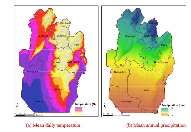
The climate shows a relatively constant mean annual temperature of 28°C. The average maximum daily temperature changes along the elevation gradient from 25°C in the northeast mountainous area to 33°C in the southwest. The minimum temperature varies from 20°C in the hottest months of December and January to 15°C during June-August. Figure 2a provides the mean daily temperature of our study area. Rain falls mostly in a bimodal pattern across the region, with the long rain during February to April, and short rain in October to November. The rain may happen as one long period mainly in the northeast or the short rain can entirely fail, especially in the southwest. The mean annual rainfall patterns show a strong gradient with less than 400mm in the southwest and with above 1000mm in the northeast as shown in Figure 2b. Although there are two main rainy seasons, the pattern and distribution of rainfall varies between months and years across the Zone.
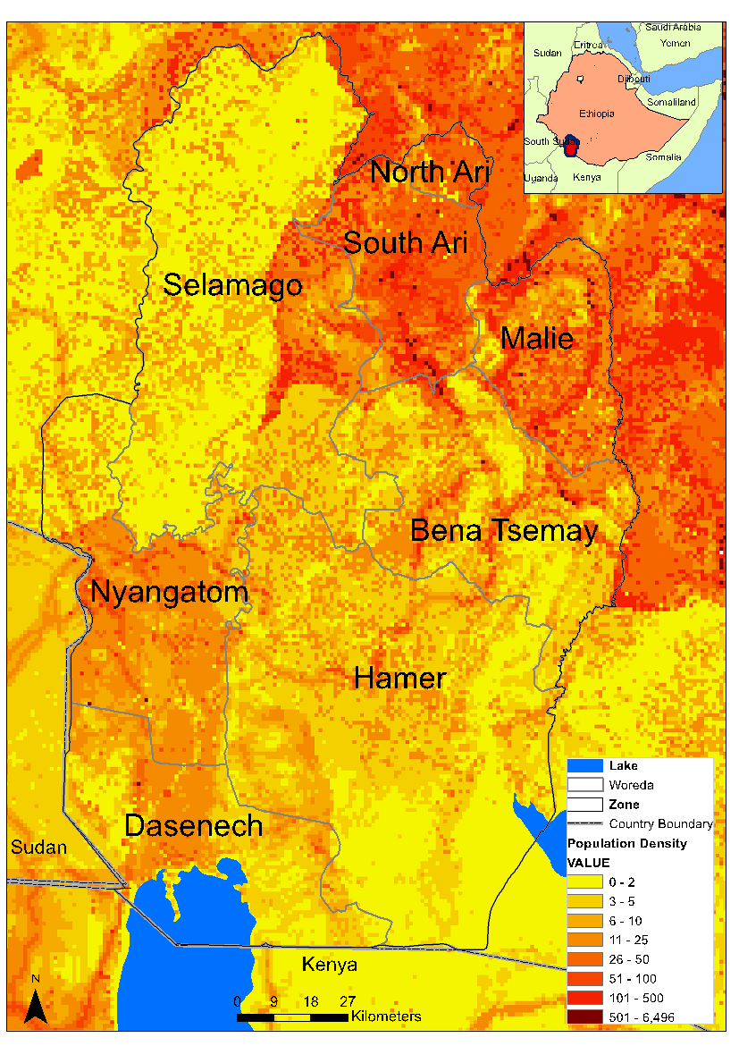
Based on the 2007 Census, the total population of the Zone is 569,448, of which 284,781 (50.01%) are males and 284,667 (49.99%) are females (CSA 2012). The total number of households is 125,009 with an average household size of 4.6. Of these, about 80% are male-headed households while the rest, 20%, are female-headed households. Figure 3 shows the population density of the Zone and although the Zone is less populated (on average 24 person per km2) when compared to the rest of the country, there is an increasing trend in population growth. For example, in 2007 the population had increased 75% from 1994.
The economic activity of the Zone is characterized by subsistence agriculture dominated by agro-pastoral and pastoral systems. The crop production system is dominated by a subsistence rain-fed crop production system, mainly targeted at filling the household consumption need. The agricultural cycle follows the two rainy seasons. Planting of staple crops (e.g., maize and sorghum) starts with the onset of the main rainy season (February - June). Staple crops planted in February are harvested in August or September depending on the length of growing period of the crop. The secondary agricultural season commences with the onset of the short rainy season that starts in September and ends in December. Supplementary crops produced in the Zone during this period, mainly in the higher altitudes, include: sorghum, wheat, barley, and teff. The average land-holding for crop production ranges from 0.1 to 2.0 hectares. Livestock production occurs mainly in the lowland areas, where moisture is a constraint. In these areas, households realize 80% of their income from the sale of livestock. The main livestock species reared are cattle, goats, and sheep, in that order of importance. Wealth is particularly gauged by cattle ownership: the better-off households have up to 70 cattle and up to about 200 small stock (about 70 Tropical Livestock Units (TLU)), while the poor have not more than 5 cattle and 25 small stock (about 6 TLU) (Gebresenbet & Kefale 2012).
The communities of the South Omo Zone have managed resources and their livelihood in the face of challenging climatic condition for many generations. They have applied different coping mechanisms, such as increasing herd size, diversifying herds and crops, and migrating in some instances. However, the change in climate variation and frequent incidence of extreme climate events affect the biophysical and socioeconomic dynamics of the Zone and challenge the adaptive capacity of the communities, as their livelihood is mainly dependent on a climate-driven agriculture production system.
The OMOLAND-CA model
We conceptualized our study area—i.e., the South Omo Zone of Ethiopia—as a coupled human and natural system (CHANS) composed of a set of interrelated agents interacting at different spatial and temporal scales. Figure 4 illustrates the main model components and their relationships. The main agents represent individual households living in a subsistence agricultural system (herding or farming) in the biophysical environment of the study area, consisting of 146.7 by 224.7 km (i.e., the South Omo Zone) using a spatial resolution of 100 by 100 m (i.e., 1 hectare). The biophysical system dynamically responds to climate dynamics (e.g., more rain generates more vegetation). Such a response will indirectly influence land-use choices by households. Climate is represented primarily by rainfall and includes patterns from seasonal normal to extreme events (e.g., drought). The model’s temporal resolution is one day, with some processes occurring when necessary conditions are satisfied. For example, crops are instantiated and grow when a household agent sows crop seeds on the household’s farmland. Similarly, a household member’s age increases once in a year. Table 1 provides an overview and description of entities (agents and other objects), their attributes, and default values. The model was implemented in the MASON simulation system, including its geographical information system (GIS) extension, GeoMASON (Luke et al. 2005; Sullivan et al. 2010). OMOLAND-CA source code, all data reported in this paper (including GIS files), and a fully detailed description of the model using the Overview, Design concepts, and Details plus Decision (ODD+D) protocol (Müller et al. 2013) are available at https://www.comses.net/codebases/5734/releases/1.1.0/, which should be sufficient for replications, extensions, and additional experimentation by others. An overview of the model’s overall structure and processes is provided in the sequel, following a shortened and modified version of the ODD+D protocol. In addition, to get a sense of the dynamics within the model a short movie of a simulation can be seen at https://youtu.be/sbAUPhOe3fk.

| Entities [Objects] | Attributes | Units | Default value or range of values | References | |
| Global model | Initial number of households | 50,000 | |||
| Household birth rate | 0.02 | CSA (2012) | |||
| Household death rate | 0.07 | CSA (2012) | |||
| Climate | Adaptive household learning rate [γ] | 0.05 | Brooks et al. (2005), Deressa et al. (2009), Gebresenbet and Kefale (2012) | ||
| Household ingenuity level [ϕ] | 0.2 -1.0 | ||||
| Cognitive bias [ξ] | 0.2 | ||||
| Intensity of cognitive [η] adaptation elasticity | 0.2 | ||||
| Cost of adaptation | 0.2 | ||||
| Risk elasticity [ζ] | 0.4 | ||||
| Percentage of initial number of adopters | % | 5 | |||
| Risk assessment exponent [x] | 0..2 | ||||
| Adaptation appraisal coefficients | α | 0.35 | |||
| β | 0.35 | ||||
| γ | 0.3 | ||||
| Herds/herding activities | Daily consumption rate | kg/TLU | 3 | Galvin (2009), Schmidt and Verweij (1992) | |
| Average livestock price | birr/TLU | 1600 | |||
| Daily consumption rate | kg/TLU | 3 | Galvin (2009), Schmidt and Verweij (1992) | ||
| Proportion of destocking rate | 0.1 | ||||
| Livestock growth rate [β] | 0.0008 | ||||
| Livestock biomass index [ν] | 0.5 | ||||
| Daily maximum dry matter (DM) intake | kg | 7 | Galvin (2009), Mulindwa et al. (2009), Schmidt and Verweij (1992) | ||
| Maximum DM stored | kg | 350 | |||
| Proportion of restocking rate | 0.1 | McCabe (1987) | |||
| Herd splitting threshold | 0.3 | ||||
| Minimum vision range | km | 50 | |||
| Maximum vision range | km | 200 | |||
| Proportion labor to Topical Livestock Unit (TLU) | person/TLU | 5 | Mulindwa et al. (2009) | ||
| Farms/farming activities | Farm Cobb-Douglas coefficient | 0.5 | |||
| Farm input cost | birr/ha | 200 | Demeke et al. (2004), Kebede et al. (1990), Terefe et al. (2010) | ||
| Farm labor efficiency factor | 1.1 | ||||
| Irrigation farm cost | birr | 200 | |||
| Intensification status | True or false | true | |||
| Maximum days to wait after land preparation | days | 30 | |||
| Minimum annual rainfall for crop production | mm | 400 | Allen et al. (1998) | ||
| Proportion labor to farmland (HA) | person/ha | 0.7 | |||
| Vegetation | Weeding day after planting | days | 30 | ||
| Base growth rate controller [φ] | 2.39 | Bekure et al. (1991), | |||
| Minimum rainfall amount | mm | 0.125 | Galvin (2009) | ||
| Maximum vegetation per hectare | kgDM/ha | 4000 | |||
| Minimum vegetation per hectare | kgDM/ha | 50 | |||
| Crops | Number of days with minimum rainfall | days | 3 | Omotosho et al. (2000) | |
| Number of days with minimum effective rainfall | days | 15 | |||
| Minimum cessation rainfall threshold | mm | 10 | |||
| Minimum effective rainfall (MER) | mm | 40 | |||
| Minimum days onset rainfall threshold | days | 10 |
Model processes, overview, and scheduling
The model sequence routine includes all components involved in the scheduling routine. Each procedure is activated by the responsible actor or entity, and at each time step similar sequential procedures are activated in the same order. The first routine concerns climate, which produces rain falling on land parcels, which, in turn, updates their level of soil moisture. For simplicity, there is no overflow, inflow of water, or accumulation of soil moisture, so the update mechanism is relatively simple. If there is no rain in a given month, a parcel’s soil moisture is assigned value zero; otherwise soil moisture in a given parcel equals the amount of rain received. However, if a parcel is irrigable, then soil moisture remains constant, regardless of the amount of rain (i.e., we assume that farmers who use irrigation will maintain an amount of soil moisture that maximizes crop growth). After a rainfall update, the vegetation subroutine is executed, by growing or shrinking (on parcels where it already exists), depending on moisture available (as detailed in Section 3.9 below).
The second routine concerns households (details in Sections 3.2-3.7). At each time step, each household conducts livelihood activities, updates its profiles, and assesses the success or failure of its actions. As shown in Figure 5, the main sequential procedures of household are: prediction of future climate conditions based on past experiences; analysis of adaptive response; selection of potential livelihood options; allocation of resources; implementation of livelihood-related activities; monitoring wealth status; updating profile; and updating memory. Routines are only executed at appropriate times under specific conditions. For instance, sequential procedures from the prediction of future climate conditions to the determination of livelihood options are executed once in any given season, based on the rainfall pattern. At the specified prediction time, the household predicts the onset and amount of rainfall for the upcoming season (see Section 3.2). Based on the outcome of its action, a household decides whether or not to adapt in response to anticipated climatic conditions for the season (see Section 3.2).
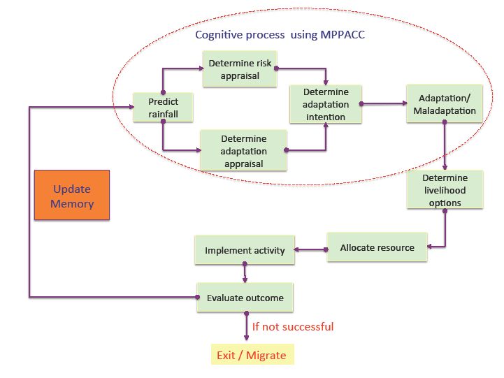
Each household chooses its adaptation strategy by combining herding and farming, in some proportion, depending on what yields the highest return (see Section 3.3). Given a chosen combination, a household then proportionately allocates resources to each. A household remembers its decision and allocation of resources for each livelihood throughout the implementation of each subsequent activity (see Section 3.4). Each activity is carried out until it has either been discarded or completed. Each household updates its memory at the end of each season (see Section 3.7).
After the household routine, the herd sequence is invoked (as detailed in Section 3.8). Herds consume grass at their current location and move to another location, updating their metabolic rate, food level, and size based on grass consumed. Next, the crop sequence is invoked at parcels where it exists (detailed in Section 3.9). Similar to vegetation, crops grow or shrink depending on moisture at their parcel. At each time step, a crop updates its growth and production level. Finally, an observer object, which collects statistics, is invoked and the output is written to a disk for further analysis.
Household socio-cognitive processes
The socio-cognitive adaptive behavior of a household in OMOLAND-CA follows the MPPACC framework of Grothmann and Patt (2005) applied to our geographic and demographic data, which uses Protective Motivation Theory (Maddux & Rogers 1983) to explain the subjective adaptive capacity of individuals to climate change. The MPPACC includes agents’ perceptions of their own capacity to adapt to climate change, a feature commonly overlooked in conventional adaptation studies, and has been applied to diverse geographic regions (e.g., Germany, Zimbabwe, and Kiribati; Grothmann & Patt 2005; Kuruppu & Liverman 2011). Its potential for ABM has been discussed but not yet fully implemented (Kniveton et al. 2011; Smith et al. 2011), so we apply it for the first time in OMOLAND-CA. We begin the implementation of MPPACC by framing the way individual households perceive future climatic conditions for proactive adaptive response, to which we turn next.
Climate forecast
Households that are entirely or partially dependent on rain-fed livelihoods predict future rainfall patterns based on past experience, proactively responding to possible impacts of climatic variability. Households predict the onset and amount of rain for each season based on past experience, assigning greater weight to recent events.
Within the model, the onset date is determined by analyzing the intensity and duration of rainfall in a given season, as defined by Omotosho et al. (2000). We first determine mean onset frequency in the South Omo Zone using 109 years (1901-2009) of rainfall data. This onset frequency is considered as a reference onset and is used as an input in the model. In the same way, the observed seasonal onset is calculated for each parcel in the same manner, assessing whether the current onset is observed early, on time, or late, and the observation is compared to the reference (long-term mean) onset. If the current season is earlier than the mean by a margin of 7 days, it is considered an "Early Onset (EO)." If the current onset occurs after the mean onset by a margin of 7 days, it is considered a "Late Onset (LO)." Otherwise, it is considered a "Normal Onset (NO)." Total seasonal rainfall is calculated to determine moisture level, by adding the amount of daily rain in each season. Seasonal rainfall variation is calculated from the long-term mean (based on the 109-year reference) and categorized into three ordinal levels: “Below Normal (BN)” if less than the reference amount by a margin set as parameter; "Above Normal (AN)" if greater than the reference amount by a margin set as parameter; or "Normal Amount (NA)". A household predicts current onset as follows:
| $$O_c = \max \sum_{i = 1}^n \sum_{j = 1}^m O_i \beta_i + \epsilon$$ | (1) |
| $$A_c = \max \sum_{i = 1}^n \sum_{j = 1}^m A_i \psi_i + \epsilon$$ | (2) |
Risk assessment
Risk assessment in the MPPACC framework has two sub-components: perceived probability and perceived severity. Perceived probability is a person’s expectation of being exposed to a threat, while perceived severity is the personal assessment of how harmful the consequence would be if the threat actually happens (Grothmann & Patt 2005).
OMOLAND-CA implements risk assessment as follows. Perceived probability is determined by a household’s confidence level when predicting current rainfall, while perceived severity is determined by potential impact of the current climate pattern (i.e., onset and amount) on agricultural practices. Therefore, following Grothmann and Patt (2005), a household assesses risk by combining perceived probability and severity, calculated as follows:
| $$R = \frac{1}{1 + \exp \bigl(-x (P * S - \zeta) \bigr)}$$ | (3) |
Adaptation appraisal
Adaptation appraisal in the MPPACC framework has three components: perceived adaptation efficacy, perceived self-efficacy, and perceived cost efficacy (Grothmann & Patt, 2005). Perceived adaptation efficacy indicates a household’s estimated effectiveness of its adaptive measures for averting threats, and is a function of household attributes (age, sex, income, education level, access to technology, and household size). Several studies (e.g., Deressa et al. 2009; Mertz et al. 2009; Nhemachena & Hassan 2007) indicate that household size, age of the household head, wealth (both monetary and livestock size), and access to technology are significant in determining the adaptive capacity of rural households in most African countries in general, and in Ethiopia in particular.
Perceived self-efficacy denotes a person’s perceived ability to perform adaptive responses, and relates particularly to a household’s past experience in responding to climate variability, which is acquired through experience or learning (Grothmann & Patt 2005; Kaufmann et al. 2009). Perceived cost efficacy denotes the cost of applying adaptive responses, and is related to agriculture production costs. These three factors affect the adaptation appraisal of a household in different ways. An increase in perceived adaptation and perceived self-efficacy increases adaptation appraisal, while an increase in perceived cost efficacy decreases adaptation appraisal. Accordingly, adaptation appraisal is calculated as follows:
| $$A_A = \alpha A_E + \beta E - \gamma C_E$$ | (4) |
Adaptation intention and decision
A strength of the MPPACC model is that it explicitly distinguishes between intention and actual behavioral adaptation (Grothmann & Patt 2005). Adaptation intention focuses on an individual’s intent to adapt, while behavioral adaptation is an individual’s actual implementation of adaptation measures. Adaptation intention refers to an individual’s estimated consequence of risk and adaptation, calculated as follows:
| $$A_I = \frac{1}{1 + \exp [-b (\mu R * A_A - \xi)]}$$ | (5) |
A household’s realization of intention depends on a threshold. If adaptation intention is lower than the threshold, maladaptation occurs; if equal or greater, then adaptation will be implemented. When maladaptation occurs, the household applies the same measure every season, so maladaptive agents will not realistically differentiate between current and normal climate conditions, behaving as though rainfall in each season were "normal." By contrast, adaptive households consider possible alternatives to minimize climate variability risk, allocating resources within their capacity, in line with climate variability.
Climate change experience and learning
Rural households can learn about climate variability and potential adaptive measures from past experiences, by imitation, or from instructors (Kaufmann et al. 2009). However, because training and farm extension activities are limited, rural households usually acquire knowledge about climate change impacts from their experience and by imitating neighbors (Kniveton et al. 2011). In the model, if a household is willing to apply adaptation measures, the household will tend to learn more from more experienced neighbors. A household’s adaptation experience is expressed as follows:
| $$E_t = E_{t - 1} + \gamma \phi \Psi \frac{H_{ADP}}{H_T} + \epsilon$$ | (6) |
Livelihood options
Households in the model sustain their livelihood by engaging in farming and/or herding, as in the real world (Gebresenbet & Kefale 2012). Since, in the South Omo Zone, off-farm activity is very limited and its contribution to household income is negligible (Gebresenbet & Kefale 2012), it is not considered as a livelihood option in this model. Income generated from either or both is determined by the amount of household labor applied to each activity, household assets (i.e., farmland, livestock), climatic conditions, and biophysical environment conditions. Households that allocate necessary inputs for each livelihood option receive more return than those who do not.
Farming households execute activities such as land preparation, planting, and harvesting. To accomplish these and allocate needed resources, households determine a date for executing each activity. The preparation date is determined by a household’s expectation of rain onset (as discussed in Section 3.2.1). Households that expect early rains will prepare their farmland earlier than will others. After land preparation, households search for the best time to plant crops. Since planting requires sufficient moisture for crops to germinate, estimating the planting date is critical for crop production in rain-fed agriculture (Ati et al. 2002; Laux et al. 2009; Odekunle et al. 2005). After determining an onset date, a household chooses a date with at least a small amount of moisture equivalent to minimum effective rain (MER), and considers this as the ideal planting date. The final farming activity is harvesting. Households harvest their crop anytime the crop reaches its length of growing period (LGP). The date chosen for harvesting depends on the urgency of the household to collect their harvest. At harvesting time, the household calculates its farm income and updates its wealth status in proportion to total yield produced.
Herding activity relates to livestock production. Within the model, herds are fed only by grazing, and herds’ movement in search of grazing is considered to be an adaptive mechanism (Coppolillo 2000; McCabe 1990). Households decide where to move in order to increase productivity and minimize hazards by considering vegetation level and proximity of the grazing area to their campsite. Households keep close to their campsite during a good wet season, but can move far in search of better vegetation in a bad dry season. Within the model, we assume that adaptive households possess a better understanding of their surrounding environment than do maladaptive households, since the latter have limited vision and information about their surrounding areas. Adaptive agents have information about vegetation conditions in distant locations and adjust their travel distance by comparing vegetation in the surrounding area with that in other areas. This simplification is not unrealistic. For instance, McCabe (2004) found that herders with greater adaptive capacity travel longer distances in time of drought than those households who do not have sufficient resources. Each household calculates the income it can receive from its herd.
Labor allocation
Within the model, a household’s labor requirement is covered by its own members. However, the allocation of labor—in a given period and to each activity—depends on a household’s attributes and environmental situation. For instance, labor allocation is a function of farmland for crop production, number of livestock, family size, climatic condition, amount of available labor, and household’s wealth status. Each household determines the proportion of labor to be allocated for a given livelihood option by comparing the expected return of each livelihood option (i.e., herding, farming). Household labor allocation to each livelihood option is proportional to expected return.
Consumption and change in wealth
A household accumulates wealth produced by all livelihood options, meeting minimal nutritional subsistence requirements. In addition to consumption expenses, households may have other expenses directly related to livelihood activities. Such expenses are occasional and demand-based. For instance, farming households opting for adaptation may have to spend on fertilizer, high-yield seeds, or new farmland. Similarly, herding households who opt to adapt must spend to restock their herd. Each day, households calculate their net accumulated wealth as:
| $$W_t = W_{t - 1} + R_t - E_t$$ | (7) |
Crop production
Crop growth depends on soil, water, air, and sunlight (Allen et al., 1998). In the model this is simplified by having crop growth depend only on water and soil quality (fertility), as follows:
| $$G_t = G_{t - 1} + \omega q m$$ | (8) |
Crop yield is determined by crop growth rate, length of growing period, and crop management, as follows:
| $$Y = G_t \, q k a l$$ | (9) |
Update memory
At the end of each season, households update their memory. Each household compares its predictions of climate indices with the observed climate situation of the season and makes appropriate changes to its memory. As households update their memory, they discard the oldest information because their memory capacity is limited (Kennedy 2012).
Livestock production
Livestock is modeled as a single herd unit and is measured as a Tropical Livestock Unit (TLU), a common measure used throughout the region (Gryseels 1988). In the model, livestock reproduce or die depending on the household management capacity and availability of forage, which in turn depends on weather, soil quality, and number of livestock consuming forage at a given time. The livestock size at a given time is given by:
| $$H_t = H_{t - 1} + \beta v l \alpha$$ | (10) |
Vegetation growth
Vegetation growth depends on the amount of moisture and soil fertility. In this study, only rainfall is considered as the main factor that influences grass growth, but the influence of soil and other factors is covered by using elevation and normalized difference vegetation index (NDVI) data as a proxy (see Gulden et al. 2011). Eq 11 is determined as:
| $$V_t = V_{t - 1} + \phi \gamma R_f \Biggl(1 - \frac{V_{t - 1}}{V_{\max}} \Biggr) $$ | (11) |
Simulation Results
Model setting and scenarios
Before presenting the model scenarios and results, we feel that it is important to discuss our attempts for model verification. Verification is the process of ensuring that a simulation is implemented as intended by the conceptual model (Crooks & Heppenstall 2012). Verification of OMOLAND-CA was performed by conducting four procedures: code walkthroughs, debugging, profiling, and parameter sweeps. These tests insured that we made no logical errors in the translation of the model into code and there were no programming errors. No anomalies have been detected since the above verification procedures were carried out, so we feel confident that the model behaves as it is intended and it matches its design.
We now move onto a set of scenarios designed to answer our research questions. As the South Omo Zone has exhibited various climatic shocks in the past, it is evident that the resilience of the rural households (and of the environment) is threatened by the intensity and frequency of the climatic shocks. The following scenario simulations therefore focus on exploring the effect of changes in climate indices on rural households in the South Omo Zone and how households cope with different climatic shocks. As the rainfall directly affects the environment, particularly vegetation growth and crop production (as discussed in Section 3, the possibility of sustaining large human and livestock populations varies with climate variation. In particular, we focus our analysis on understanding how climate change affects the adaptive capacity of rural households, and how they might manage to survive under extreme climatic events. Below we report on four scenarios that answer our research questions. These are as follows, in order of increasing realism: (1) a base scenario based on “normal” climate conditions, (2) the effect of rare extreme events on rural households, (3) the effects of consecutive extreme events on rural households, and finally (4) the effect of erratic extreme climatic events, which resembles the real rainfall pattern of the study area.
In scenario 1 we began the simulation by creating a mean annual rainfall with “normal” onset and amount for the entire region. We generated the mean annual rainfall by calculating the mean of 109 years (1901 to 2009) of monthly rainfall data. We assume that this mean annual rainfall is an indicator of the “normal” (or “good year”) climatic conditions for the region and consider it as the baseline scenario. We then ran the simulation keeping this mean annual rainfall the same every year, indicating that the climate condition of the region is “normal.” By carrying out this scenario our intention was to help us understand how rural households interact with the environment and how their characteristics and livelihood decision-making affect their probability of survival (or their success). Moreover, it allowed us to explore the carrying capacity of the environment to sustain the livestock and human population under “normal” climatic situations.
In the second scenario, we introduced droughts as extreme events. We assessed three different frequencies of drought: a drought every 5, every 10, or every 15 years. For each occurrence of drought, we assessed the following severity levels: 50%, 70%, and 90% from changes to the mean. In each extreme event year, we decreased the rainfall amount by the assigned severity level from the mean annual rainfall while keeping the other years “normal.” Due to the nature of the model, any change in climate, particularly the occurrence of extreme events, will affect the growth of crops and grasses, and ultimately affect rural households by enhancing or disrupting their production systems. This scenario therefore allows us to explore the resilience of rural households to such events and their capacity to respond. By doing this, we explored the implications of extreme climatic events on the adaptive capacity of rural households. In the third scenario, we increased the frequency of extreme events by allowing consecutive occurrences; i.e., droughts occurring for two consecutive years in every 5, 10, or 15 years. Our aim with this scenario was to explore the implication of consecutive occurrences of extreme events: specifically, how a household’s resource base might be altered by extreme events and to what extent a household copes with long-term extreme events.
Finally, the fourth scenario explored rural households’ resilience to “real life” erratic climatic conditions. The actual rainfall pattern of the study area is erratic and incorporates both good and bad years. It shows high variation not only year to year but also month to month. We used actual rainfall patterns of the Zone for this scenario. We utilized 50 years of rainfall data from 1949 to 2009. We chose 50 years as consistent with most other agent-based land-use and land-cover change models (Entwisle et al. 2008; Parker et al. 2003).
In each scenario, the main agents considered were the rural households residing in the South Omo Zone. All simulation runs were for 18,250 iterations (each iteration step is a day and 18,250 iterations are approximately 50 years). We ran a set of 30 simulations for each scenario and report the mean value of these runs (default values are presented in Table 1). In the next section we report specifically on the livestock crops and population changes.
Results
(1) Base scenario under "normal" climate situation
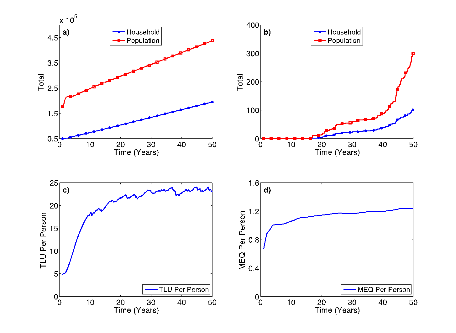
Under a “normal year” scenario, household numbers increased over time and reached 155,916 after 50 years, as shown in Figure 6a. The total population increased by 47% over the simulation period and the population density changed from 0.03 to 0.16 people per sq. kilometers. The “normal” climatic condition throughout the simulation favored both livestock and crop production. As shown in Figure 4c, per capita livestock numbers increased sharply in the first 10 years and started stabilizing as they reached ecological capacity. The trend in crop production also showed an ascending trend, but not as significantly as livestock, as indicated in Figure 6d. The overall success of households under this climatic scenario can be seen by monitoring the rate of migration over the simulation period. Figure 6b shows the number of households and population migrating from the system due to loss of wealth. Although population density increased over time, households seem favored by the “normal” climatic condition and all but a few were able to sustain their livelihood. However, as the simulation period continued, households with large family sizes were especially vulnerable to migration as their resource base was easily diminished through consumption, even though the climate conditions were relatively normal.
(2) The effect of rare extreme events on rural households
In the second scenario, we introduced droughts with various intensity and frequency to explore the adaptive capacity of rural households. The impact of extreme climatic events on rural households was pronounced as frequency and intensity increased. The impact can be seen clearly as we account for the number of people who migrated to nearby towns, as shown in Figure 7. A change in climate clearly affected households, especially when droughts occurred over shorter periods. Households who did not accumulate wealth to support them beyond a year were forced to leave their area and migrate to nearby towns as more episodes of drought occurred.

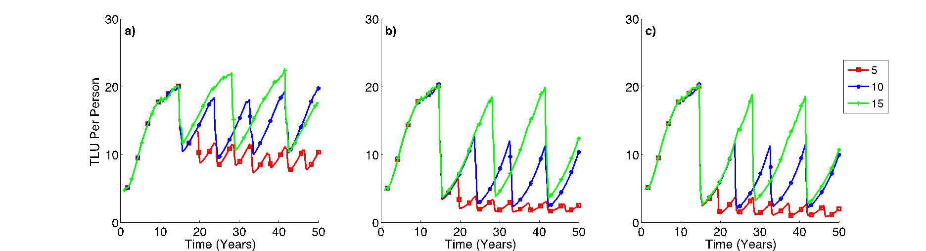
Droughts also affected livestock numbers in the system. Change in TLU per person was dramatic, as the frequency and intensity of droughts increased. Although the droughts occurred once every 15 years, the TLU per person decreased by 30% to 90% as intensity increased from 50% to 90% as shown in Figure 8a, b, and c. However, as the simulation progressed, the numbers slowly recovered and reached 20 TLU per person as a consequence of more “normal” or favorable climatic years, until the next drought year occurred. Another striking result was the impact of a drought as it occurred more frequently. In the situation where a drought occurred once every 5 years, the number of TLU per person decreased dramatically and was difficult to recover from, because livestock growth depends on the amount of vegetation available in the surrounding area, which is highly correlated with rainfall amount.
(3) Consecutive extreme events on rural households
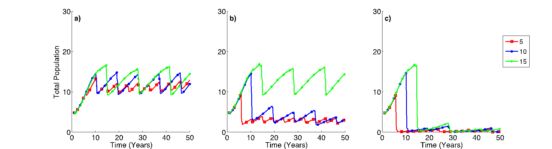
Because droughts often last longer than a year, we incorporated this in the model. In Figure 9 and 10, one can see how prolonged droughts affected the asset capital of rural households, forcing them to migrate rapidly as the simulation progressed under different frequencies of occurrences. In all cases, the number of people migrating in this scenario was significantly greater than in scenario 2. For instance, as compared to scenario 2, about 35,000 additional people migrated in scenario 3 when drought occurred for two consecutive years in every 10 years with 90% intensity. The impact of such types of multi-year drought events can drain households’ resources for coping and recovery. Hence, households could no longer sustain their livelihood and were forced to migrate in significant numbers.

(4) The effect of erratic extreme climatic events
In the "real world," climatic conditions are unpredictable; in our study area there are some good and some bad years with pronounced occurrences of drought. Such erratic rainfall patterns have a direct implication for the rural household decision-making and their productive systems, particularly with respect to crop and livestock production. The implication of this can be seen as we observe the model results from “erratic years” scenario runs (Figure 11). Population and household numbers increased over time as the simulation progressed (Figure 11a), as was the case in scenario 1. However, now the rate of growth slowed as the number of households migrating to nearby towns increased over time (Figure 11b).
Another surprising result from this scenario was the trend of livestock and crop production in the Zone. As shown in Figure 11c, TLU per person decreased over time while MEQ per person showed an increasing trend (Figure 11d). A similar observation was reported by Samuel (2013): most pastoralists in the South Omo Zone are increasingly adopting cultivation to compensate for livestock losses. This can be explained by the unpredictable nature of the rainfall pattern, which affected the recovery rate of livestock per household and, therefore, more households were encouraged to engage in crop production. Although more households engaged increasingly in crop production, the spatial distribution of crop pattern in the Zone was not homogenous. Even in areas where the biophysical and climate conditions were similar, the choice of each household to engage in farming showed significant variation as shown in Figures 12 and Figure 13.
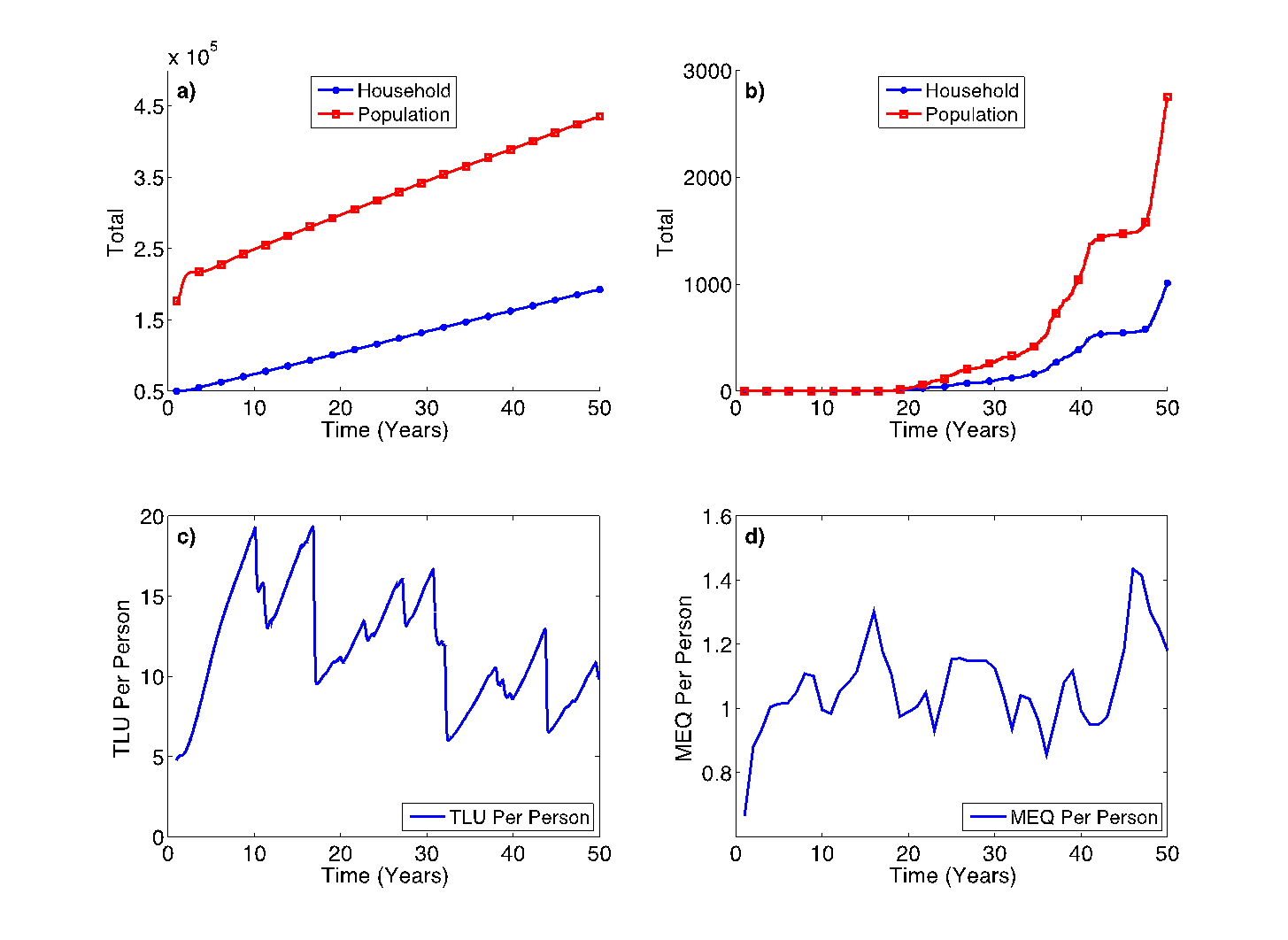
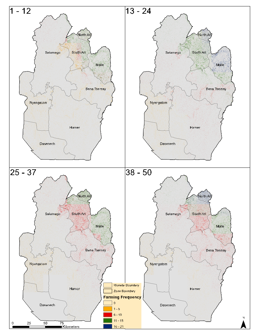
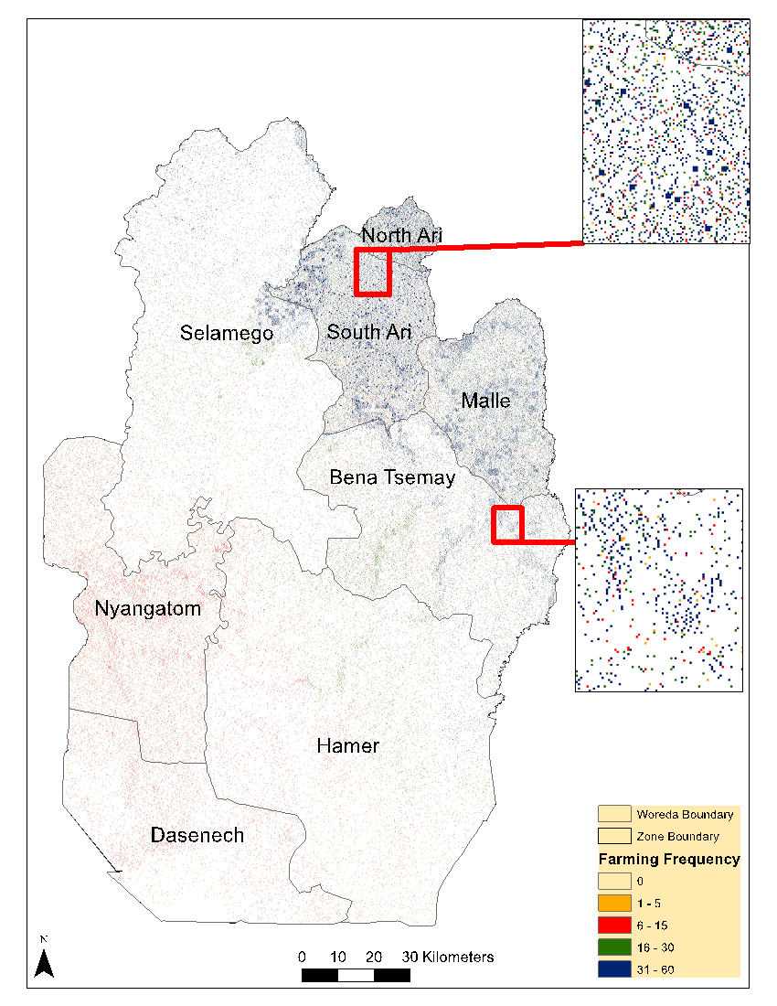
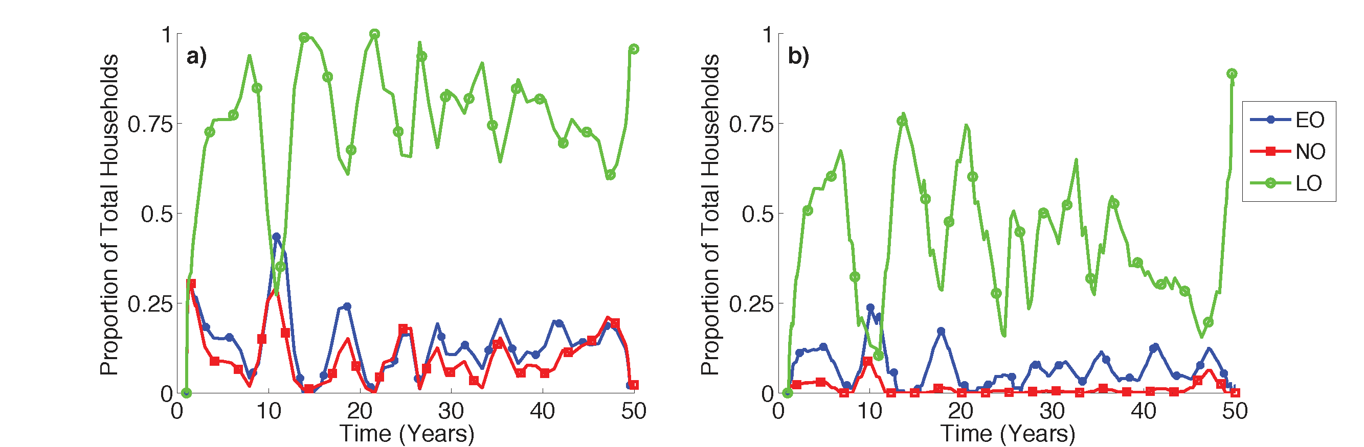
Figure 14 allows us to assess how rural households within the model made their predictions and how their judgment aligns with the real seasonal rainfall outlook. Specifically, Figure 10b shows that almost throughout the simulation period, more than 60% of the rural households predicted the onset of rainfall as late onset, while the rest predicted the seasonal outlook of rainfall as normal or early onset. When we compare how much their prediction aligns with the real seasonal pattern of the rainfall, the proportion significantly lowered to below 50% in most simulation periods, with a few exceptions.
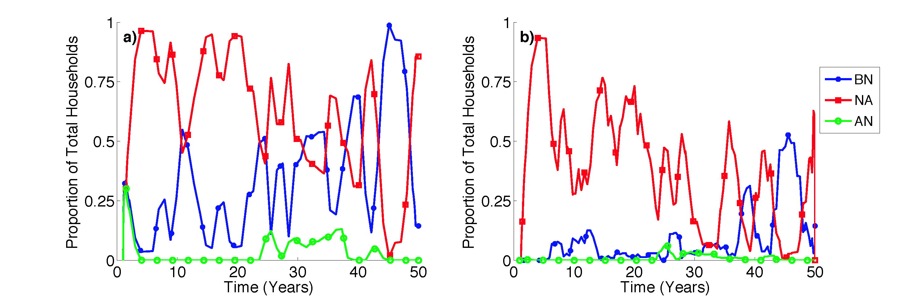
The prediction of the amount of seasonal rainfall is shown in Figure 15. In the first 30 years of the simulation period, the proportion of households that predicted seasonal rainfall as “normal” accounted for more than 50% of the total households. However, the number dropped significantly after 30 years, as most of the households assumed the rainfall amount likely to be below normal. The level of accuracy of household prediction of the amount of rainfall, however, showed a declining trend as the variability of the rainfall increased over time. As shown in Figure 15b, the proportion of rural households that correctly predicted based on past experience was higher in the first 30 years than in the last 20 years. As discussed in Section 3.3.1, a rural household forecasts seasonal rainfall based on the previous three years of rainfall for the season. Due to limited access to public climate prediction information and high dependency on traditional prediction methods, the probability of a rural household accurately forecasting both rainfall onset and amount is very low. Such an information flaw ultimately affects the way in which rural households respond to climate variability.
Discussion and Conclusions
In brief, our results provide answers to the research questions that motivated the OMOLAND-CA model, as follows: Under which climate change conditions are households pushed beyond the limits of survival? Under conditions that exceed current erratic changes in the frequency and intensity of drought events? How do various mixes of herding and farming affect household well-being under climate change conditions? Undoubtedly, mixed strategies provide a superior survival advantage for households facing the harsh challenges of climate change in the Omo Zone and similar environments. What role do factors such as households’ ability to accurately predict weather events have on livelihoods and adaptation to climate change? A critical role is played by a household’s ability to accurately predict drought changes, although accomplishing this is very difficult. Each answer has important details and caveats, as demonstrated by simulation results in the four scenarios created for answering our research questions. Climate change has the potential to greatly affect the socioeconomic dynamics of rural households that rely on subsistence agricultural systems. In the South Omo Zone of Ethiopia, rural household livelihoods depend heavily on rain-fed agriculture systems and any variation in climate can affect the population in many ways. The OMOLAND-CA model presented in this paper demonstrates how climate variability influences the dynamics of such a rural population through the operationalization of the MPPACC framework. The model suggests that rural households’ adaptation to climate change is highly influenced by their adaptive capacity and their expectation of future climatic situations. While the rural communities in the South Omo Zone are better off in normal climate conditions, and they can survive if the current climate conditions persist. The occurrence of successive episodes of extreme events even after good climatic years, however, results in substantial damage to their assets (livestock and crop) and consequently affects their adaptive capacity, forcing them to migrate to nearby towns in greater numbers. The model also demonstrates that rural households could achieve a strong resource base with relatively continuous good climate years. Such accumulation of resources assists rural households to withstand droughts which have a high degree of intensity.
The magnitude of livestock losses under severe extreme climatic events reported in scenarios 2 and 3 are not uncommon in pastoral areas such as the South Omo Zone. Previous studies (e.g., McCabe 1987, 2004; Oba 2001) have shown that in times of severe drought, livestock losses can reach 90%. For instance, McCabe (1987) investigated livestock losses for four pastoral families in Turkana, Kenya, during the drought of 1979-1983, reporting losses of 63% cattle, 45% camels, and 55% small stock with respect to total family possession before the drought. Moreover, droughts can also reduce the number of rural households, by triggering migration to nearby cities to seek employment (Oba 2001).
Rural households utilize different mechanisms to forecast the onset and amount of seasonal rainfall. In most cases, they base their prediction on rainfall pattern of previous years (Luseno et al. 2003). The OMOLAND-CA model captures such rural household forecasting behavior by mapping previous rainfall patterns to the decision-making of the households on when to start the next cropping activities. However, in the “real world,” due to limited access to public climate prediction information and high dependency on their traditional prediction methods, the chance of the rural household accurately forecasting the rainfall onset and amount is very low (Luseno et al. 2003), consistent with our simulation results. Such an information flaw ultimately affects the way the rural households respond to climate variability.
Our modeling approach complements current efforts in agent-based modeling, specifically with respect to representing richer socio-cognitive behavior of agents along with integrating geographical information systems (GIS) into such models. This represents a significant methodological thrust in computational social science and geospatial modeling more generally (Crooks & Heppenstall 2012). The OMOLAND-CA model explicitly represented the socio-cognitive behavior of agents, and utilized various spatial datasets to represent the different model entities. However, there are still gaps that need to be addressed to develop a better understanding of the adaptive behavior of rural households when challenged by climate change. The current model passes face-validity tests, since its processes and outcomes are reasonable and plausible (see Hailegiorgis 2013 for more details). Efforts were also made to ensure the model matched existing spatial and demographic patterns in the Zone, and the rules of the agents were based on what is ethnologically known about the inhabitants of the area (as discussed in Section 3). However, more rigorous empirical validation is necessary to ensure the robustness of the emerging patterns and their dynamic nature. The challenge here, which is seen in many similar agent-based models, is that there is often not enough data to carry out such validation and this is compounded for models that are developed in less developed countries where data scarcity is even more prevalent (Mahabir et al. 2016). Future directions for model development should therefore focus on improving behavioral representations of rural households with regards to seasonal climate outlooks and adaptation strategies, along with more widespread data collection. For instance, it would be interesting to explore the willingness of rural households to adopt new agricultural technology and climate adaptation measures, as rural systems are likely to be influenced by the emergence of new technologies, market opportunities, financial incentives, and land-use policies (Kaufmann et al. 2009). It would also be interesting to explore how rural households’ trust and their reactions to information pertaining to seasonal climate outlooks, particularly from meteorological centers of the region, as improved information on seasonal climate outlooks could play an important role in the adaptation responses of rural communities (Bharwani et al. 2005), thereby mitigating effects of climate change.
Finally, although we did not model directly the demographic dynamics of households, we did model births and deaths in individual households, which affects the amount of labor assigned to each livelihood option. Family cohesion and cooperation in forming a large group might be another adaptive mechanism among agropastoral societies. This is another potential direction for future research with OMOLAND. From the above discussion, it is clear that many avenues of future research are possible; however, this study plays an important role in pioneering these issues and laying foundations for additional work to capture the complex dynamics of coupled human-natural systems under conditions of climate change.
Acknowledgements
This work was supported by the US National Science Foundation through a Doctoral Dissertation Research Improvement (NSF-DDRI) grant (no. 112348), a Cyber-Enabled Discovery and Innovation (CDI) Program grant (no. IIS-1125171), by the Office of Naval Research (ONR) under a Multi-disciplinary University Research Initiative grant (no. N00014-08-1-092), and by the Center for Social Complexity at George Mason University. The opinions, findings, and conclusions expressed in this work are those of the authors and do not necessarily reflect the views of the sponsors. The authors would like to thank the editor and two anonymous reviewers for comments and suggestions which improved the quality of the paper.References
ACOSTA-MICHLIK, L., & Espaldon, V. (2008). Assessing vulnerability of selected Farming Communities in the Philippines based on a behavioural model of agent's adaptation to global environmental change. Global Environmental Change, 18(4), 554-563. [doi:10.1016/j.gloenvcha.2008.08.006]
ADGER, W. N., Dessai, S., Goulden, M., Hulme, M., Lorenzoni, I., Nelson, D. R., et al. (2009). Are there social limits to adaptation to climate change? Climatic Change, 93(3-4), 335-354.
ADMASU, T., Abule, E., & Tessema, Z. (2010). Livestock-rangeland management practices and community perceptions towards rangeland degradation in South Omo zone of Southern Ethiopia. Livestock Research for Rural Development, 22(1), 5. http://www.lrrd.org/lrrd22/1/tere22005.html.
AGRAWAL, A., & Perrin, N. (2009). 'Climate adaptation, local institutions and rural livelihoods.' In W. N. Adger, I. Lorenzoni & K. L. O'Brien (Eds.), Adapting to Climate Change: Thresholds, Values, Governance. Cambridge, UK: Cambridge University Press, pp. 350-367.
ALLEN, R. G., Pereira, L. S., Raes, D., & Smith, M. (1998). Crop evapotranspiration-guidelines for computing crop water requirements. Rome. Italy: Food and Agriculture Organization of the United Nations, Irrigation and Drainage Paper 56.
ARAYA, A., Stroosnijder, L., Girmay, G., & Keesstra, S. D. (2011). Crop coefficient, yield response to water stress and water productivity of Teff (eragrostis tef (zucc.). Agricultural Water Management, 98(5), 775-783.
ATI, O. F., Stigter, C. J., & Oladipo, E. O. (2002). A comparison of methods to determine the onset of the growing season in Northern Nigeria. International Journal of Climatology, 22(6), 731-742. [doi:10.1002/joc.712]
BALKE, T., & Gilbert, N. (2014). How do agents make decisions? A survey. Journal of Artificial Societies and Social Simulation, 17(4), 13: https://www.jasss.org/17/4/13.html. [doi:10.18564/jasss.2687]
BEKURE, S., de Leeuw, P. N., Grandin, B. E., & Neate, P. J. H. (Eds.). (1991). Maasai Herding: An Analysis of the Livestock Production System of Maasai Pastoralists in Eastern Kajiado District, Kenya. Addis Ababa, Ethiopia: International Livestock Centre for Africa.
BERGER, T. (2001). Agent-based spatial models applied to agriculture: A simulation tool for technology diffusion, resource use changes and policy analysis. Agricultural Economics, 25(2-3), 245-260.
BERGER, T., & Troost, C. (2014). Agent-based modelling of climate adaptation and mitigation options in agriculture. Journal of Agricultural Economics, 65(2), 323-348. [doi:10.1111/1477-9552.12045]
BERT, F., North, M., Rovere, S., Tatara, E., Macal, C., & Podestá, G. (2015). Simulating agricultural land rental markets by combining agent-based models with traditional economics concepts: The case of the Argentine Pampas. Environmental Modelling & Software, 71, 97-110.
BHARWANI, S., Bithell, M., Downing, T. E., New, M., Washington, R., & Ziervogel, G. (2005). Multi-agent modelling of climate outlooks and food security on a community garden scheme in Limpopo, South Africa. Philosophical Transactions of the Royal Society of London B: Biological Sciences, 360(1463), 2183-2194. [doi:10.1098/rstb.2005.1742]
BOMMEL, P., Dieguez, F., Bartaburu, D., Duarte, E., Montes, E., Machín, M. P., et al. (2014). A further step towards participatory modelling. Fostering stakeholder involvement in designing models by using executable UML. Journal of Artificial Societies and Social Simulation, 17(1), 6: https://www.jasss.org/17/1/6.html. [doi:10.18564/jasss.2381]
BROOKS, N., Adger, W. N., & Kelly, P. M. (2005). The determinants of vulnerability and adaptive capacity at the national level and the implications for adaptation. Global Environmental Change, 15(2), 151-163. [doi:10.1016/j.gloenvcha.2004.12.006]
BRYAN, E., Deressa, T. T., Gbetibouo, G. A., & Ringler, C. (2009). Adaptation to climate change in Ethiopia and South Africa: Options and constraints. Environmental Science & Policy, 12(4), 413-426.
CIOFFI-REVILLA, C. (2016). 'Socio-Ecological Systems.' In William S. Bainbridge & Mihail C. Roco (Eds.), Handbook of Science and Technology Convergence. New York and Heidelberg: Springer, pp. 669-689. [doi:10.1007/978-3-319-07052-0_76]
CIOFFI-REVILLA, C., Rogers, J. D., & Latek, M. (2010). 'The MASON HouseholdWorld model of pastoral nomad Societies.' In K. Takadama, C. Cioffi-Revilla & G. Deffaunt (Eds.), Simulating Interacting Agents and Social Phenomena: The Second World Congress in Social Simulation. Berlin, Germany: Springer, pp. 193-204.
CIOFFI-REVILLA, C., Rogers, J. D., Schopf, P, Luke, S., Bassett, J. K., Hailegiorgis, A. B., & Wei, E. (2015). MASON NorthLands: A geospatial agent-based model of coupled human-artificial-natural systems in Boreal and Arctic Regions. Paper presented at the Social Simulation Conference 2015, Groningen, The Netherlands, 14-18 September 2015.
COOPER, P. J. M., Dimes, J., Rao, K. P. C., Shapiro, B., Shiferaw, B., & Twomlow, S. (2008). Coping better with current climatic variability in the rain-fed farming systems of Sub-Saharan Africa: An essential first step in adapting to future climate Change? Agriculture, Ecosystems & Environment, 126(1), 24-35.
COPPOLILLO, P. B. (2000). The landscape ecology of pastoral herding: Spatial analysis of land use and livestock production in East Africa. Human Ecology, 28(4), 527-560. [doi:10.1023/A:1026435714109]
CROOKS, A. T., & Heppenstall, A. (2012). 'Introduction to agent-based modelling.' In A. Heppenstall, A. T. Crooks, L. M. See & M. Batty (Eds.), Agent-based Models of Geographical Systems. New York, NY: Springer, pp. 85-108.
CSA. (2012). The 2007 Population and Housing Census of Ethiopia: Statistical Report for Southern Nations, Nationalities and Peoples' Region. Vol. 1. Addis Ababa, Ethiopia: Central Statistics Agency of Ethiopia.
DEADMAN, P. J., Robinson, D. T., Moran, E., & Brondizio, E. (2004). Effects of colonist household structure on land use change in the Amazon rainforest: An agent based simulation approach. Environment and Planning B, 31(5), 693-709.
DEMEKE, M., Guta, F., & Ferede, T. (2004). Agricultural Development in Ethiopia: Are There Alternatives to Food Aid? Addis Ababa, Ethiopia: Department of Economics, Addis Ababa University. Available at: http://sarpn.org/documents/d0001583/FAO2005_Casestudies_Ethiopia.pdf.
DERESSA, T. T., Hassan, R. M., Ringler, C., Alemu, T., & Yesuf, M. (2009). Determinants of farmers' choice of adaptation methods to climate change in the Nile basin of Ethiopia. Global Environmental Change, 19(2), 248-255.
ENTWISLE, B., Malanson, G., Rindfuss, R. R., & Walsh, S. J. (2008). An agent-based model of household dynamics and land use change. Journal of Land Use Science, 3(1), 73-93. [doi:10.1080/17474230802048193]
EPSTEIN, J. M. (2008). Why model? Journal of Artificial Societies and Social Simulation, 11(4), 12: https://www.jasss.org/11/4/12.html.
ERIKSEN, S. H., Brown, K., & Kelly, P. M. (2005). The Dynamics of vulnerability: Locating coping strategies in Kenya and Tanzania. The Geographical Journal, 171(4), 287-305. [doi:10.1111/j.1475-4959.2005.00174.x]
ETIENNE, M., Le Page, C., & Cohen, M. (2003). A step-by-step approach to building land management scenarios based on multiple viewpoints on multi-agent system simulations. Journal of Artificial Societies and Social Simulation, 6(2), 2: https://www.jasss.org/6/2/2.html.
FILATOVA, T., Voinov, A., & van der Veen, A. (2011). Land market mechanisms for preservation of space for coastal ecosystems: An agent-based analysis. Environmental Modelling & Software, 26(2), 179-190. [doi:10.1016/j.envsoft.2010.08.001]
FUNK, C., Dettinger, M. D., Michaelsen, J. C., Verdin, J. P., Brown, M. E., Barlow, M., et al. (2008). Warming of the Indian Ocean threatens Eastern and Southern African food security but could be mitigated by agricultural development. Proceedings of the National Academy of Sciences, 105(32), 11081-11086. [doi:10.1073/pnas.0708196105]
GALVIN, K. A. (2009). Transitions: Pastoralists living with change. Annual Review of Anthropology, 38, 185-198.
GEARD, N., McCaw, J. M., Dorin, A., Korb, K. B., & McVernon, J. (2013). Synthetic population dynamics: A model of household demography. Journal of Artificial Societies and Social Simulation, 16(1), 8: https://www.jasss.org/16/1/8.html. [doi:10.18564/jasss.2098]
GEBRESENBET, F., & Kefale, A. (2012). Traditional coping mechanisms for climate change of pastoralists in South Omo, Ethiopia. Indian Journal of Traditional Knowledge, 11(4), 573-579.
GROTHMANN, T., & Patt, A. (2005). Adaptive capacity and human cognition: The process of individual adaptation to climate change. Global Environmental Change, 15(3), 199-213. [doi:10.1016/j.gloenvcha.2005.01.002]
GRYSEELS, G. (1988). Role of Livestock on Mixed Smallholder Farms in the Ethiopian Highlands: A Case Study from the Baso and Worena Wereda Near Debre Berhan. PhD Dissertation, Agricultural University, Wageningen, The Netherlands.
GULDEN, T., Cotla, C. R., Hailegiorgis, A., & Crooks, A. T. (2011). A generic vegetation growth sub-model in a large human/environment interaction model of East Africa. Paper presented at the Computational Social Science Society of America Conference (2011).
HAILEGIORGIS, A. (2013). Computational Modeling of Climate Change, Large-scale Land Acquisition, and Household Dynamics in Southern Ethiopia Doctoral Dissertation. Computational Social Science, George Mason University, Fairfax, VA.
HAILEGIORGIS, A., Kennedy, W., Roleau, M., Bassett, J., Coletti, M., Balan, G., et al. (2010). An Agent Based Model of Climate Change and Conflict among Pastoralists in East Africa. Paper presented at the 2010 International Congress on Environmental Modelling and Software Modeling for Environment's Sake, Ottawa, Canada.
KAUFMANN, P., Stagl, S., & Franks, D. W. (2009). Simulating the diffusion of organic farming practices in two new EU member states. Ecological Economics, 68(10), 2580-2593. [doi:10.1016/j.ecolecon.2009.04.001]
KEBEDE, Y., Gunjal, K., & Coffin, G. (1990). Adoption of new technologies in Ethiopian agriculture: The case of Tegulet-Bulga district Shoa province. Agricultural Economics, 4(1), 27-43.
KELLY, R. A., Jakeman, A. J., Barreteau, O., Borsuk, M. E., ElSawah, S., Hamilton, S. H., Henriksen, H. J., Kuikka, S., Maier, H. R., Rizzoli, A. E., van Delden, H. & Voinov, A. A(2013). Selecting among five common modelling approaches for integrated environmental assessment and management. Environmental Modelling & Software, 47, 159-181. [doi:10.1016/j.envsoft.2013.05.005]
KENNEDY, W. (2012). 'Modelling human behaviour in agent-based models.' In A. Heppenstall, A. T. Crooks, L. M. See & M. Batty (Eds.), Agent-based Models of Geographical Systems. New York, NY: Springer, pp. 167-180.
KNIVETON, D., Smith, C., & Wood, S. (2011). Agent-based model simulations of future changes in migration flows for Burkina Faso. Global Environmental Change,21(Supplement 1), S34-S40. [doi:10.1016/j.gloenvcha.2011.09.006]
KNIVETON, D. R., Schmidt-Verkerk, K., Smith, C., & Black, R. U. N. (2008). Climate Change and Migration: Improving Methodologies to Estimate Flows. Geneva, Switzerland: International Organization for Migration, IMO Migration Research Series No. 33.
KURUPPU, N., & Liverman, D. (2011). Mental preparation for climate adaptation: The role of cognition and culture in enhancing adaptive capacity of water management in Kiribati. Global Environmental Change, 21(2), 657-669. [doi:10.1016/j.gloenvcha.2010.12.002]
LAUX, P., Jäckel, G., Tingem, M., & Kunstmann, H. (2009). 'Onset of the rainy season and crop yield in Sub-Saharan Africa - Tools and perspectives for Cameroon.' In T. M.C., K. Heal, E. Bagh, A. Chambel & V. Smakhtin (Eds.), Ecohydrology of Surface and Groundwater Dependent Systems: Concepts, Methods and Recent Developments (pp. 191-200). Hyderabad, India: International Association of Hydrological Sciences.
LEE, J. S., Filatova, T., Ligmann-Zielinska, A., Hassani-Mahmooei, B., Stonedahl, F., Lorscheid, I., et al. (2015). The complexities of agent-based modeling output analysis. Journal of Artificial Societies and Social Simulation, 18(4), 4: https://www.jasss.org/18/4/4.html. [doi:10.18564/jasss.2897]
LIU, J., Dietz, T., Carpenter, S. R., Alberti, M., Folke, C., Moran, E., Pell, A. N., Deadman, P., Kratz, T., Lubchenco, J., Ostrom, E., Ouyang, Z., Provencher, W., Redman, C. L., Schneider, S. H. & Taylor, W. W.(2007). Complexity of Coupled Human and Natural Systems. Science, 317(5844), 1513-1516.
LUKE, S., Cioffi-Revilla, C., Panait, L., Sullivan, K., & Balan, G. (2005). MASON: A multi-agent simulation environment. Simulation, 81(7), 517-527. [doi:10.1177/0037549705058073]
LUSENO, W. K., McPeak, J. G., Barrett, C. B., Little, P. D., & Gebru, G. (2003). Assessing the value of climate forecast information for pastoralists: Evidence from Southern Ethiopia and Northern Kenya. World Development, 31(9), 1477-1494.
MADDUX, J. E., & Rogers, R. W. (1983). Protection motivation and self-efficacy: A revised theory of fear appeals and attitude change. Journal of Experimental Social Psychology, 19(5), 469-479. [doi:10.1016/0022-1031(83)90023-9]
MAHABIR, R., Crooks, A.T., Croitoru, A. & Agouris, P. (2016). The study of slums as social and physical constructs: Challenges and emerging research opportunities. Regional Studies, Regional Science, 3(1), 737-757.
MCCABE, J. T. (1987). Drought and recovery: Livestock dynamics among the Ngisonyoka Turkana of Kenya. Human Ecology, 15(4), 371-389. [doi:10.1007/BF00887997]
MCCABE, J. T. (1990). Turkana pastoralism: A case against the tragedy of the commons. Human Ecology, 18(1), 81-103.
MCCABE, J. T. (2004). Cattle Bring Us to Our Enemies. Ann Arbor, MI: University of Michigan Press. [doi:10.3998/mpub.23477]
MCCARTHY, J. J., Canziani, O. F., Leary, N. A., Dokken, D. J., & White, K. S. (Eds.). (2001). Climate Change 2001: Impacts, Adaptation, and Vulnerability: Contribution of Working Group II to the Third Assessment Report of the Intergovernmental Panel on Climate Change. Cambridge, UK: Cambridge University Press.
MENDELSOHN, R., & Dinar, A. (1999). Climate change, agriculture, and developing countries: Does adaptation Mmatter? The World Bank Research Observer, 14(2), 277-293. [doi:10.1093/wbro/14.2.277]
MERTZ, O., Mbow, C., Reenberg, A., & Diouf, A. (2009). Farmers' perceptions of climate change and agricultural adaptation strategies in Rural Sahel. Environmental Management, 43(5), 804-816.
MORTIMORE, M. J., & Adams, W. M. (2001). Farmer adaptation, change and `crisis' in the Sahel. Global Environmental Change, 11(1), 49-57. [doi:10.1016/S0959-3780(00)00044-3]
MORTON, J. (2007). The impact of climate change on smallholder and subsistence agriculture. Proceedings of the National Academy of Sciences, 104(50), 19680-19685.
MORTON, J., McPeak, J., & Little, P. (2006). 'Pastoralist coping strategies and emergency livestock market intervention.' In J. G. McPeak & P. D. Little (Eds.), Pastoral Livestock Marketing in Eastern Africa: Research and Policy Challenges. London, UK: Intermediate Technology Publications Ltd, pp. 227-246. [doi:10.3362/9781780440323.013]
MULINDWA, H., Galukande, E., Wurzinger, M., Mwai, A. O., & Sölkner, J. (2009). Modelling of long term pasture production and estimation of carrying capacity of Ankole pastoral production system in South Western Uganda. Livestock Research for Rural Development, 21(9), 151: http://lrrd.cipav.org.co/lrrd21/9/muli21151.html.
MÜLLER, B., Bohn, F., Dreßler, G., Groeneveld, J., Klassert, C., Martin, R., et al. (2013). Describing human decisions in agent-based models – ODD + D, An Extension of the ODD Protocol. Environmental Modelling & Software, 48, 37-48. [doi:10.1016/j.envsoft.2013.06.003]
NHEMACHENA, C., & Hassan, R. (2007). Micro-Level Analysis of Farmers Adaptation to Climate Change in Southern Africa. Washington, DC: International Food Policy Research Institute, IFPRI Discussion Paper 00714.
NIAMIR-FULLER, M. (2000). 'Managing mobility in African rangelands.' In N. McCarthy, B. Swallow, M. Kirk & P. Hazell (Eds.), Property Rights, Risk, and Livestock Development in Africa. Washington, D.C: International Food Policy Research Institute, pp. 102-131.
OBA, G. (2001). The effect of multiple droughts on Cattle in Obbu, Northern Kenya. Journal of Arid Environments, 49(2), 375-386.
ODEKUNLE, T. O., Balogun, E. E., & Ogunkoya, O. O. (2005). On the prediction of rainfall onset and retreat dates in Nigeria. Theoretical and Applied Climatology, 81(1-2), 101-112. [doi:10.1007/s00704-004-0108-x]
OMOTOSHO, J. B., Balogun, A. A., & Ogunjobi, K. (2000). Predicting monthly and seasonal rainfall, onset and cessation of the rainy season in West Africa using only surface Data. International Journal of Climatology, 20(8), 865-880.
OSBAHR, H., Twyman, C., Adger, W. N., & Thomas, D. S. (2008). Effective livelihood adaptation to climate change disturbance: Scale dimensions of practice in Mozambique. Geoforum, 39(6), 1951-1964. [doi:10.1016/j.geoforum.2008.07.010]
PARKER, D. C., Manson, S. M., Janssen, M. A., Hoffmann, M. J., & Deadman, P. (2003). Multi-agent systems for the simulation of land-use and land-cover change: A review. Annals of the Association of American Geographers, 93(2), 314-337.
PUTRA, H. C., Zhang, H., & Andrews, C. (2015). Modeling real estate market responses to climate change in the coastal zone. Journal of Artificial Societies and Social Simulation, 18(2), 18: https://www.jasss.org/18/2/18.html. [doi:10.18564/jasss.2577]
RINDFUSS, R. R., Entwisle, B., Walsh, S. J., An, L., Badenoch, N., Brown, D. G., Deadman, P., Evans, T. P., Fox, J., Geoghegan, J., Gutmann, M., Kelly, M., Linderman, M., Liu, J., Malanson, G. P., Mena, C. F., Messina, J. P., Moran, E. F., Parker, D. C., Parton, W., Prasartkul, P., Robinson, D. T., Sawangdee, Y., Vanwey, L. K. & Verburg, P. H.(2008). Land use change: Complexity and comparisons. Journal of Land Use Science, 3(1), 1-10.
SAMUEL, T. (2013). From cattle herding to sedentary agriculture: The role of hamer women in the transition. African Study Monographs, 46, 121-133.
SAQALLI, M., Gérard, B., Bielders, C. L., & Defourny, P. (2011). Targeting rural development interventions: Empirical agent-based modeling in Nigerien villages. Agricultural Systems, 104(4), 354-364.
SCHMIDT, A. M., & Verweij, P. A. (1992). 'Forage intake and secondary production in extensive livestock systems.' In H. Balslev & J. L. Luteyn (Eds.), Páramo. An Andean Ecoystem under Human Influence (pp. 197-210). London, UK: Academic Press.
SMIT, B., Burton, I., Klein, R. J., & Wandel, J. (2000). An anatomy of adaptation to climate change and variability. Climatic Change, 45(1), 223-251.
SMIT, B., & Skinner, M. (2002). Adaptation options in agriculture to climate change: A typology. Mitigation and Adaptation Strategies for Global Change, 7(1), 85-114. [doi:10.1023/A:1015862228270]
SMITH, C., Kniveton, D. R., Wood, S., & Black, R. (2011). 'Climate change and migration: A modelling approach.' In C. J. R. Williams & D. R. Kniveton (Eds.), African Climate and Climate Change: Physical, Social and Political Perspectives. New York, NY: Springer, pp. 179-201.
SOLOMON, S. Qin, D., Manning, M., Averyt, K. & Marquis, M. (2007). Climate Change 2007 - The Physical Science Basis: Working Group I Contribution to the Fourth Assessment Report of the IPCC. Cambridge, UK: Cambridge University Press.
SULLIVAN, K., Coletti, M., & Luke, S. (2010). GeoMason: GeoSpatial Support for MASON. Fairfax, VA: Department of Computer Science, George Mason University, Technical Report Series.
TEREFE, A., Ebro, A., & Tessema, Z. K. (2010). Rangeland dynamics in South Omo Zone of Southern Ethiopia: Assessment of rangeland condition in relation to altitude and grazing types. Livestock Research for Rural Development, 22(10), 187: http://www.lrrd.org/lrrd22/10/tref22187.html.
THORNTON, P. K., Van de Steeg, J., Notenbaert, A., & Herrero, M. (2009). The impacts of climate change on livestock and livestock systems in developing countries: A review of what we know and what we need to know. Agricultural Systems, 101(3), 113-127. [doi:10.1016/j.agsy.2009.05.002]
YOHE, G., & Tol, R. S. (2002). Indicators for social and economic coping capacity: Moving toward a working definition of adaptive capacity. Global Environmental Change, 12(1), 25-40.