Youth and Their Artificial Social Environmental Risk and Promotive Scores (Ya-TASERPS): An Agent-Based Model of Interactional Theory of Delinquency

and
aGeorge Mason University, United States; bUniversity at Buffalo, United States
Journal of Artificial
Societies and Social Simulation 24 (4) 2![]()
<https://www.jasss.org/24/4/2.html>
DOI: 10.18564/jasss.4660
Received: 19-Nov-2020 Accepted: 05-Jul-2021 Published: 31-Oct-2021
Abstract
Risk assessments are designed to measure cumulative risk and promotive factors for delinquency and recidivism, and are used by criminal and juvenile justice systems to inform sanctions and interventions. Yet, these risk assessments tend to focus on individual risk and often fail to capture each individual’s environmental risk . This paper presents an agent-based model (ABM) which explores the interaction of individual and environmental risk on the youth. The ABM is based on an interactional theory of delinquency and moves beyond more traditional statistical approaches used to study delinquency that tend to rely on point-in-time measures, and to focus on exploring the dynamics and processes that evolve from interactions between agents (i.e., youths) and their environments. Our ABM simulates a youth’s day, where they spend time in schools, their neighborhoods, and families. The youth has proclivities for engaging in prosocial or antisocial behaviors , and their environments have likelihoods of presenting prosocial or antisocial opportunities. Results from systematically adjusting family, school, and neighborhood risk and promotive levels suggest that environmental risk and promotive factors play a role in shaping youth outcomes. As such the model shows promise for increasing our understanding of delinquency.Introduction
Many countries, especially European countries, set the age of criminal responsibility (i.e., when a child/youth can be held accountable for their behavior) at age 14 (Hazel 2008). This coincides with a peak period of offending in adolescence (called the age-crime curve), when offending may be considered somewhat normative before tapering off in adulthood (Agnew 2003). For the youth who may be engaged in “normative” adolescent behavior but get in trouble with the law, many actually do have complex, unmet social service needs (Lee & Taxman 2020; Maschi et al. 2008). They often live in high-risk social contexts, including family, schools, and neighborhoods, as evidenced by their higher rates of adverse childhood experiences (Baglivio et al. 2014) and mental health disorders (Abram et al. 2003; Teplin et al. 2002). Moreover, they report higher rates of unmet social and psychological service needs than the general population (Maschi et al. 2008), and many report negative outcomes well into adulthood (Abram et al. 2017; Barnert et al. 2019).
These youth have been the focus of many scholars, who have produced an extensive range of theories explaining the etiology of deviance, crime, and delinquency that tend to highlight either individual, social, or societal predictors (for an example, see (Jacoby et al. 2004)). More recently, there have been efforts to move beyond the etiology of deviance to develop theories that also explain the persistence or desistance of deviant behavior (Sampson & Laub 1997; Thornberry 1987). In spite of the richness of existing theories to explain deviance, crime, and delinquency, many of these theories have not been used to guide practice. Perhaps this is because less is known about the specific mechanisms that are operating within these theories, or how interventions might affect those mechanisms. Rather, the criminal justice field has adopted the risk factor prevention paradigm from public health (Farrington et al. 2016), resulting in a strong focus on identifying risk and promotive factors as a guide for determining the sanctions and interventions the court requires (Hilterman et al. 2014).
In part, this may be due to the methods that have been traditionally used to test these theories thus far. While criminologists arguably have exhausted cross sectional approaches, scholars have advocated for the use of longitudinal methods in order to study the development of delinquency (Loeber & Le Blanc 1990). Yet, longitudinal methods are expensive and not always used effectively, and still pose limitations in the knowledge that can be developed about dynamic processes, such as establishing causal effects between variables and, even when identified, revealing the causal mechanisms (Farrington 2015; Gottfredson & Hirschi 1987; Loeber & Le Blanc 1990). This paper seeks to integrate both theory and practice by incorporating a risk and promotive approach into an interactional theory of delinquency using agent-based modeling. ABM is a type of computer simulation that simulates the interaction of agents (i.e., individuals) with each other and with their environments over time (Lee & Wolf-Branigin 2020). In this paper we have developed an agent-based model to test an interactional theory of delinquency, which hypothesizes that delinquency results not just from individual risk, but also from their interactions with their environments (Thornberry & Krohn 2005). Youth are agents in the model with their own social environments, and their decisions contribute to future opportunities, such as the job opportunities that become available as they progress educationally (Thornberry et al. 1991). The intention of our model is to move us beyond a conceptual model of individual risk to testing both environmental risk and the interaction between individual and environmental risk (Ihara & Lee 2019).
In the reminder of this this paper we begin with a review of criminological theory and risk assessment literature and existing studies testing interactional theory of delinquency (Section 2). Within Section 2 we also explore agent-based models with respect to social work and studying delinquency before introducing our agent-based model in Section 3. Section 4 presents and discusses the results from our agent-based model, while Section 5 provides a summary of the paper and areas of further work.
Background
There has been a rich tradition of criminological theories, and classic theories of delinquency and crime have ranged from focusing on individual factors (e.g., Gottfredson & Hirschi 1990 General Theory of Crime which focused on self-control), interactions with peers (e.g., Sutherland 1947 Differential Association) and others (e.g., Lemert 1951 Labeling Theory), and social structural factors (e.g., Merton 1938 Anomie Theory). In part, this plethora of theories reflects the equifinality nature of delinquency – there are multiple routes to delinquency.
In spite of the rich tradition of criminological theories, the U.S. criminal justice system adopted the risk factor prevention paradigm from public health (Farrington et al. 2016). Thus, efforts have focused on identifying risk factors, which increase the likelihood of delinquency, crime, and recidivism, and promotive factors, which decrease the likelihood of delinquency, crime, and recidivism (Arthur et al. 2002). Often, criminal and juvenile justice systems (depending on the locale) administer standardized risk assessments to identify risk levels. Standardized risk assessments have been through multiple stages of development in the last century, moving away from expert assessments (first generation risk assessments) to the standardized risk assessments (fourth generation) that are the standard today. These fourth-generation risk assessments include both risk and promotive factors, as well as static and dynamic risk factors across 8-10 domains (Baird et al. 2013; Slobogin 2012). Domains often include legal history, school, mental health, neighborhood, peers, and family. These risk assessment domains can be further broken down into dynamic and static risk and promotive factors. For example, this results in 25 subscales that the Youth Assessment Screening Instrument (YASI) produces (Jones et al. 2016).
Many countries use some type of psychological assessments (e.g., psychological, mental health, or risk assessments) with youth when they first come in contact with the juvenile justice system in order to triage the youth and to guide decisions about punishments or treatments (Wright et al. 2019). Currently in the U.S., it has become standard practice for juvenile or criminal justice systems to administer standardized risk assessments, depending on state or county policies. While these assessments cover a comprehensive set of risk and promotive factors across multiple domains, they produce more information than most service providers and public agencies can effectively use. While the separate subscales can be an effective case management tool, they are rarely used as such (Peterson-Badali et al. 2015; Taxman & Caudy 2015). Rather, the risk assessments are summarized as a single indicator of high, medium, and low risk, which guide the number of requirements and level of supervision individuals receive. Yet, specific needs identified in the risk assessment typically do not result in services in those areas. Perhaps this is because delinquency has been described as an equifinality phenomenon – a variety of causes can lead to the same result of delinquency (Thornberry & Krohn 2005). From this perspective, it is the quantity of risk factors, not specific risk factors, that are important in predicting delinquency (Arthur et al. 2002). As a result, youth with higher risk assessment scores experience more intense sanctions (e.g., punishment).
Yet, these risk assessments focus on the individual, and thus, risk is conceptualized as a collection of characteristics or statuses that reside within the individual. These risk assessments may be incomplete in that they do not sufficiently account for interactions that may occur between the individual and other actors or their environments (Serin et al. 2016). Characteristics of the environment are significant predictors of delinquency and recidivism (Grunwald et al. 2010). For example, neighborhood measures such as neighborhood disadvantage are significantly correlated with juvenile delinquency (Rodriguez 2013; Sampson et al. 2002), which is commonly measured by a combination of factors including rates of poverty, unemployment, welfare, high school education, and female headed households; household income; and collective efficacy. Moreover, reducing an individual’s risk may not be effective if their contexts of risk do not change.
Interactional Theory: A developmental theory of process
More recently, criminologists have begun to focus on explaining the development of delinquency through adolescence by integrating various classic theories to articulate the developmental mechanisms that may be operating to produce adult criminals (Loeber & Le Blanc 1990; Sampson & Laub 1997). For example, Moffitt (1993) has argued for a developmental taxonomy, which acknowledges the heterogeneity of this population by differentiating between life-course persistent and adolescence-limited antisocial behavior. While Moffitt (1993) has focused on the role of peers in contributing to adolescent behaviors, others have provided a more general overview of how delinquency may develop, encompassing not just peers but larger social environments including the family, school, and neighborhoods. For example, Thornberry (1987), which was subsequently extended by Thornberry et al. (1991) and Thornberry & Krohn (2005), has developed an interactional theory of delinquency. The theory is based on the key assertion that “human behavior occurs in social interaction and can therefore best be explained by models that focus on the interactive process” (Thornberry 1987 p. 864). Thus, an individual’s behavioral outcomes (e.g., delinquency) cannot be understood in isolation from their social environment.
Thornberry & Krohn (2005) identify three fundamental premises to the theory. First, interactional theory of delinquency takes a developmental life-course perspective. A life course perspective acknowledges an individual’s agency while recognizing that individuals are embedded within social relationships (Elder 1994). Within this perspective, factors that contribute to the initiation, maintenance, or desistance of delinquency change during developmental periods. Thus, in childhood, the family plays a critical role in the youth’s development. In adolescence, as the youth is becoming more independent, the family plays a less important role while peers and schools begin to play a more important role (Sampson & Laub 1997; Thornberry & Krohn 2005). Moreover, it has been argued that delinquent values do not begin to form until early adolescence (Thornberry et al. 1991). Furthermore, an individual’s success in one developmental stage has implications for success in later stages (Thornberry & Krohn 2005) and therefore success in adolescence will situate the youth for a successful adulthood, and thus warrants study.
The second premise is bidirectional causality, which captures the interaction between the individual and their environment (Thornberry & Krohn 2005). Not only do factors from an individual’s social environment change the youth’s risk, but the youth’s behaviors and choices also shape the social environments in which they exist (Thornberry & Krohn 2005). The reciprocal relationship between the youth and their social environment occurs through both the interactions with individuals (e.g., parents, teachers, peers) as well as in the changing set of opportunities available to the youth. Interactions between the youth and their social environment are mutually reinforcing, resulting in behavioral trajectories (e.g., delinquency) that are path dependent (Thornberry 1987). Sampson & Laub (1997) describe this path dependency as a process of cumulative disadvantage. This process is the result of the ongoing consistency of the individual’s behaviors (cumulative continuity) as well as the responses from others that maintain the individual’s behaviors (interactional continuity) (Sampson & Laub 1997). For example, a youth who skips school actively plays a role in shaping their future opportunities – if they continue to make these choices, they may fall behind in school, which may limit their college options. At the same time, there may be maintaining responses from others such as a suspension from school or an arrest for truancy, which would contribute to the disruptions to the youth’s academic progress and thus, propel the youth on their current behavioral trajectory.
Finally the third premise of the interactional theory of delinquency is proportionality of cause and effect, which “states that as the magnitude of the causal force increases, the person’s involvement in crime (a) becomes more likely and (b) increases in severity” (Thornberry & Krohn 2005 p. 187). This approach embraces the idea of equifinality in that it is not about specific causal factors, but rather, the accumulation of causal factors (Arthur et al. 2002). Risk assessments are compatible with this third premise, since they seek to measure the accumulation of both risk and promotive factors in order to predict delinquency and recidivism, and as currently used, do not distinguish between the type of risk factor. However, current risk assessments may be limited in their ability to capture the youth’s social environments – their peer networks, the quality of their schools, the prosocial alignment of their families (Serin et al. 2016). Moreover, these risk assessments cannot capture the youth’s interactions with other individuals and their communities.
Empirical evidence supporting Interactional Theory of Delinquency
There is some empirical evidence that supports interactional theory of delinquency, yet existing statistical approaches provide only a limited test of this theory of process – even studies that use longitudinal data must rely upon point in time measures with large gaps between those measures (Hoffmann et al. 2013; Jang 1999; Lee 2003; Thornberry et al. 1991). For example, Jang (1999) tested the developmental, life-course perspective premise of interactional theory of delinquency that there are age-varying effects of family, school, and delinquent peers on adolescents. In this study, Jang (1999) used multilevel modeling with five waves of data from the National Youth Survey, and found that school and peers have a curvilinear effect while families have a consistent effect on adolescents. Such a study supports the notion that depending on the youth’s developmental stage, different factors have stronger or weaker effects.
Studies testing interactional theory of delinquency have also focused on the bidirectional causality premise. For example, Thornberry et al. (1991) used three waves of data from the Rochester Youth Development Study, and found reciprocal relationships between a youth’s bond to family and school, and engagement in delinquent behaviors. Similarly, Lee (2003) used a structural equation modeling approach with four time points from the National Youth Survey, and tested not only family, but also peers, and found that reciprocal relationships with peers play a stronger role than families. Finally, Hoffmann et al. (2013) also used structural equation modeling with two waves of Add Health data to test the reciprocal relationship between delinquency and academic achievement. They found partial support for interactional theory of delinquency where academic achievement is related to later delinquency, but delinquency is not directly related to later academic achievement (Hoffmann et al. 2013).
While such studies provide evidence to support bidirectional causality, they rely on several point-in-time estimates that are months or years apart to establish the reciprocal relationships. Thus, existing studies provide partial tests of the theory, and while they have been promising, they are limited. Using other approaches, such as agent-based modeling, may be useful in testing the generative mechanisms and provides a richer understanding of the phenomena under study by “triangulating” various approaches that have different strengths and limitations.
Risk accumulation and limitations of current approaches
Research on risk and risk assessments are not an explicit test of interactional theory of delinquency, yet provide information about how risk accumulates and operates. Studies suggest that it is the cumulative amount of risk, rather than specific factors, that are important (e.g., Arthur et al. 2002). In other words, more risk, regardless of what types of risk, increase the likelihood of delinquency or recidivism. Yet, it is less clear how risk accumulates. Standardized instruments tend to take a linear approach to risk (Arthur et al. 2002; Baglivio 2009), which assumes that each risk and promotive factor is equal and total risk can be calculated by the sum of risk and promotive factors. However, some studies indicate that there may be a linear association for some risk factors, and a nonlinear association for others (e.g., Farrington et al. 2016).
Nor is it clear how risk and promotive factors interact, which can operate in a variety of ways. In fact, promotive factors have been differentiated from protective factors. While promotive factors are conceptualized as directly reducing the likelihood of offending or recidivating (compensatory effect), protective factors interact with risk factors and operate in the presence of high risk factors (buffering effect) (Brumley & Jaffee 2016; Serin et al. 2016; Stoddard et al. 2012). Yet, these approaches focus only on predicting antisocial outcomes (offending or recidivism), and fail to take into account prosocial development and the ways that prosocial and antisocial development are intertwined. Thus, we hypothesize two separate processes, rather than a single process (Lee & Ballew 2018), where a risk factor increases the likelihood of antisocial behavior, and a promotive factor increases the likelihood of prosocial behavior.
Studies focused on risk suggest that risk clusters; there appear to be common risk profiles for youth (Lee & Taxman 2020; Onifade et al. 2008; Schwalbe et al. 2008). Some of these common risk profiles include a low needs group, a high needs group, substance use service needs, and mental health service needs (Lee & Taxman 2020). As Simon (1996) argues, “The apparent complexity of [human] behavior over time is largely a reflection of the complexity of the environment in which we find ourselves” (p. 53). Simon (1996) goes on to posit that “human goal-directed behavior simply reflects the shape of the environment in which it takes place” (p. 62). This suggests that we can infer characteristics of what a youth’s environment lacks based on what the youth needs.
Moreover, studies focused on environmental risk suggest that a youth’s environment may contribute to this clustering of risk (Rodriguez 2013). For example, one study that used spatial analysis found that recidivism clusters in certain locations (Harris et al. 2011). This suggests that risk can accumulate in the youth’s environment, and thus if we are trying to prevent recidivism, we should also take into account the youth’s environment.
Agent-based modeling as a new approach for studying delinquency
While there is evidence that a youth’s context presents risk and promotive opportunities for the youth, current approaches cannot adequately test this premise. These current limitations in existing approaches can be addressed by using agent-based modeling, which has been described as a third way of doing science, after the traditional inductive and deductive approaches (Axelrod 1997). The use of simulation has tremendous potential for studying vulnerable populations, such as those that are the focus of social work researchers (e.g., child welfare and juvenile justice involved families), since simulations can be repeated with minor adjustments. Furthermore, agent-based models move beyond identifying patterns in the data to allowing researchers to simulate the process– by systematically altering aspects of the process, we can deepen our understanding of the mechanisms that contribute to our observed outcomes (Gilbert & Troitzsch 2005).
However, while agent-based models have been developed for a wide range of applications, within the context of social work and specifically with respect to at-risk youth they have seen limited uptake. Agent-based models have been developed to explore aspects of the criminal activity (Groff 2007; Malleson et al. 2013) or the criminal justice system at large (Boyle et al. 2003), such models only look at the consequences of and not at possible interventions early on in an individual’s life. With this being written, there are growing calls for agent-based models to be used is social service research. The rationale for this, is similar to that seen in other fields such as in economics or public policy, that the world can be viewed as a complex adaptive system (Gilbert et al. 2018; Tesfatsion & Judd 2006) which allow researchers and practitioners to study the inter connections between individuals and emergent outcomes (Ihara & Lee 2019; Israel & Wolf-Branigin 2011) such as the drivers of metal health (see Langellier et al. 2019 for a review), or models exploring policies on how to reduce stress on caregivers (Kennedy et al. 2015), self-help with respect to addiction (Hiance et al. 2012) or exploring barriers to primary care for minority groups (Oh et al. 2020).
Turning to agent-based models that study youth at-risk, Schuhmacher et al. (2014) developed an agent-based model to explore how adolescents may adapt risky behaviors such as drug use or oppositional behavior on the evolution of friendships (i.e., peer interactions) at school over the course of a year. Similarly, Leaw et al. (2015) explored how youths might turn to antisocial behavior through interacting with their peers. In this model, Leaw et al. (2015) utilized ideas from Moffitt's (1993) dual taxonomy on youths’ potential for antisocial behavior based on their life courses and interactions with others and what interventions may reduce antisocial behavior among at-risk youth (e.g., changes in their social structure/network placing them in different groups, which was discussed in Section 2.1).
However, within the model presented in this paper, we focus on the environment more than their social networks as our conjecture is that the youth and their peers live in similar environments. Thus, by addressing environmental risk, we hypothesize that we can reduce the likelihood that the youth and their peers will develop antisocial behaviors (see Section 2.2). Furthermore, we would argue that just taking a youth out of one group and placing them in another does not really reduce the risk that youth face and one could argue that it is nearly impossible to orchestrate youth relationships.
Methodology
Purpose of the model
In spite of the plethora of theories on crime and delinquency, and work focused on developing risk assessments and predicting delinquency (as discussed in Section 2), it is surprising how limited our knowledge of how risk is generated and how risk operates. Thus, this study takes a stylized facts approach to model development (Garavaglia et al. 2013; Heine et al. 2005; Meyer 2011). Given the equifinality nature of delinquency (and the multitude of possible causes of delinquency), modeling delinquency is especially well-matched with a stylized facts approach, which “concentrates on broad tendencies and ignores individual details so as to identify robust patterns across different observations” (Heine et al. 2005, p. 202). This approach does not simply require predictions to be correct, but is also concerned with the accuracy of generative mechanisms (Heine et al. 2005). In this sense, the model presented in this paper offers the opportunity to make and test assumptions about how risk is generated and how risk operates, moving beyond current, broad assertions that simply more risk increases the likelihood of delinquency.
The purpose of this study is to develop an ABM based on the premises of interactional theory of delinquency which is a developmental theory of process that is based on the idea that individual outcomes are the result of an individual’s interaction with their social environment. Additionally, principles of risk and risk assessment approaches are also used in order to account for the accumulation of risk. Using a stylized facts approach, we can examine whether the model generates the broad patterns already identified empirically. If so, we can find evidence to support interactional theory.
Such a model requires both the individual and environment (i.e., 2 levels), interaction between agents (people), and for the agents (people) to be relatively complex. Thus, an ABM is well-suited to testing this theory in contrast to other simulation techniques, such as system dynamics models which do not represent individual agents, or microsimulation which does not represent interactions between agents and/or their environments, and queuing models, which do not allow for more sophisticated agents (Gilbert & Troitzsch 2005). In the agent-based model presented in this paper, youth move through their days by interacting with the three major domains of their social environments: their families, school, and their neighborhoods. This allows for the youth to be influenced by their families, schools, and peers in their neighborhoods, and thus allows us to move beyond a model of individual risk to examine how the youth’s risk is co-shaped with environmental risk.
Model description
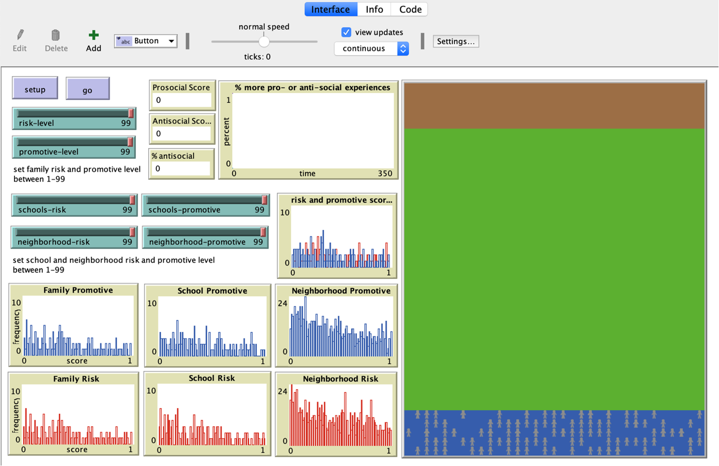
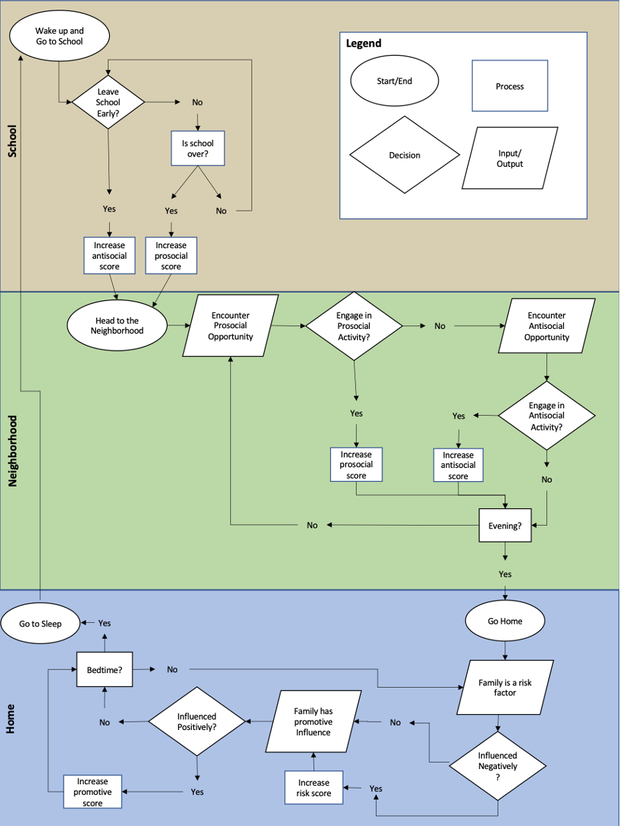
The agent-based model consists of only one type of heterogeneous agent, youths. The youth operates within a world which consists of their home (family), their schools, and their neighborhoods (peers). Throughout the course of a day, the youth faces opportunities to engage in antisocial or prosocial activities as they go to school, move through their neighborhoods, and spend time at home. When faced with opportunities, youth decide whether to engage in those opportunities based on their risk or promotive scores. The graphical user interface of the model is presented in Figure 1.
Youth and environmental characteristics
Youths are given a set of characteristics: individual risk scores and individual promotive scores, which indicate, respectively, the likelihood that a youth will engage in an antisocial or prosocial opportunity. This represents the youth’s scores on a standardized risk assessment, which include both risk scales and promotive scales (as discussed in Section 2). The higher their risk score indicates a larger accumulation of risk, which interactional theory of delinquency posits results in a stronger force for choosing to engage in antisocial opportunities (Thornberry et al. 1991). We assume that promotive factors operate the same way for prosocial behaviors, and thus, a larger accumulation of promotive factors results in a stronger force for choosing to engage in prosocial opportunities (see Section 2.2). Thus, this model assumes that risk and promotive factors operate as two independent, parallel processes – where a higher-level of risk impacts the likelihood of engagement in antisocial behavior but does not directly impact the likelihood of prosocial behavior (Farrington et al. 2016; Hoge et al. 1996). Consequently, two separate prosocial and antisocial trajectories are represented in the form of a running tally of prosocial experiences and a running tally of antisocial experiences. The model begins in early adolescence, because that is when they start to develop delinquent values (Thornberry et al. 1991). Additionally, during adolescence, family begins to play a less important role while school and peers begin to have more of an influence on youth, as young teens become more autonomous and begin to make independent decisions about their own activities (Stoddard et al. 2012; Thornberry 1987). Thus, the model includes family, school, and neighborhood locations.
The risk that youth encounter in their social environments, the family, school, and neighborhood, are modelled in two ways. First, youth are assigned their family’s risk and promotive scores. Interactional theory of delinquency posits that it is a youth’s attachment to their parents may contribute to their later delinquency (Thornberry 1987). Thus, the family’s risk and promotive scores are assigned to the youth, and the youth’s individual risk and promotive scores are derived from the family’s scores. Ultimately, whether the youth is influenced by their family is modeled as the result of a combination of the family’s scores and the youth’s individual scores.
Thornberry (1987) also posits that a youth’s commitment to school and association with delinquent peers also contributes to their delinquent behaviors. While the youth’s family represents a social environment that likely won’t change as the youth moves around in their day-to-day lives, the schools and neighborhoods represent a physical environment that does change depending on the youth’s physical location. Thus, the schools and neighborhood spaces in the model are each assigned scores for risk opportunities and prosocial opportunities. These scores are the likelihood that a youth in that location will be faced with an antisocial opportunity or a prosocial opportunity. In school, examples of these opportunities include a teacher or coach that may give a youth the opportunity to participate in an extracurricular activity (e.g., chorus, theater, or soccer), which would be a prosocial opportunity. Or, a youth may run into a peer who may encourage them to skip class or encourage them to get in trouble in class (an antisocial activity). In this way, other individuals, including peer and mentor influences, are not directly modelled, but are abstractly represented as either prosocial or antisocial opportunities. Thus, a youth faces varying levels of risk or prosocial opportunities depending on where they are at the moment.
Model initialization
Upon initialization, the artificial world is created as shown in Figure 2 A, which consists of the youths’ homes (blue), their schools (brown), and their neighborhoods (green). Due to the notion that youth’s movements are likely more restricted at home and at school, these areas are smaller than the neighborhood, where youth likely have more autonomy and a less predictable range of experiences. Figure 2 B shows youth mostly in school, with a few in the neighborhood, and Figure 2 C shows youth in the neighborhood. Thus, where the youth are determines whether they are exposed to family, school, or neighborhood risk or promotive influences. We use colors for visually debugging the model and to study interactions (Grimm 2002). At initialization, the youth are grey. If their overall tally of antisocial experiences is higher than their overall tally of prosocial experiences, they turn red, and if the reverse is true, they are green.
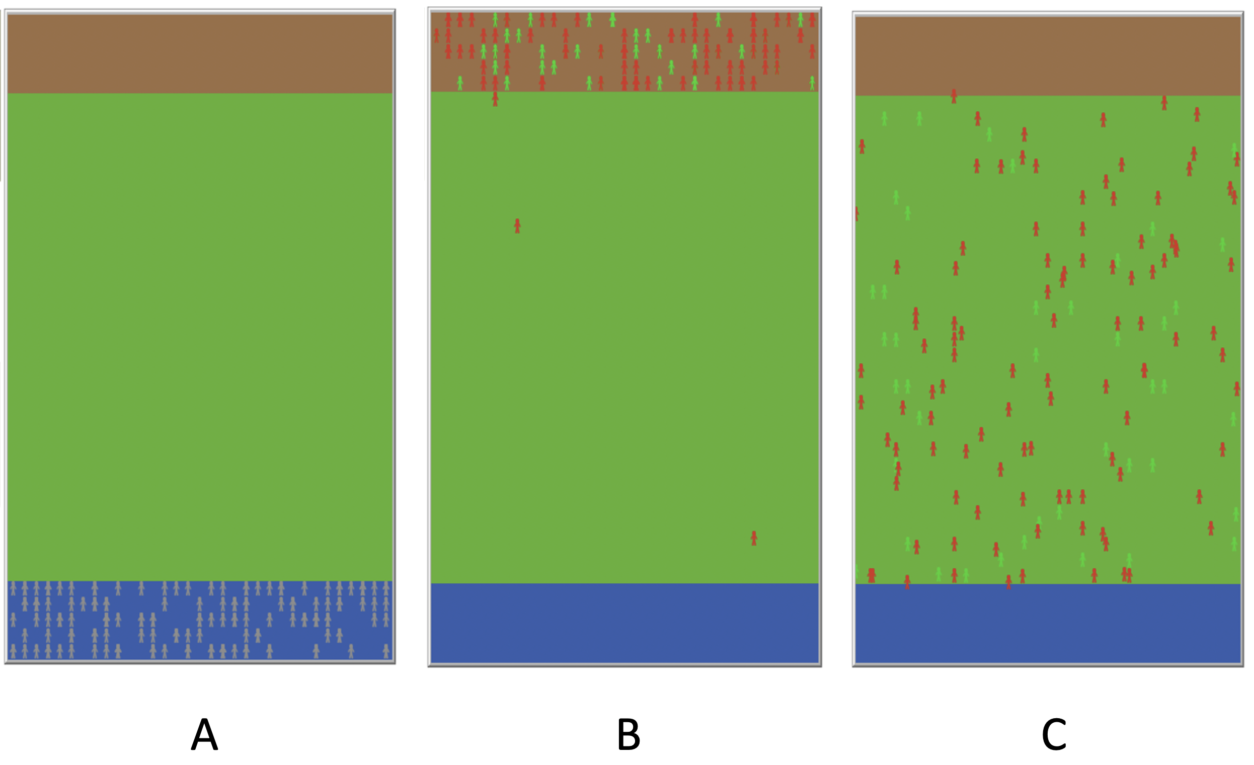
Table 1 shows the initialization values for each variable. Each school cell and neighborhood cell is assigned a probability of encountering both risk and prosocial opportunities, which can be manipulated by the user. This allows the user to systematically altered the youth’s environmental risk in order to examine the effect of each on youth outcomes (see Figure 1). Each location is given a randomized score drawn from an exponential distribution that is centered on a user-provided mean value. This is based on studies that suggest that risk tends to cluster environmentally (Harris et al. 2011; Rodriguez 2013), and thus would resemble a distribution with more low-risk locations and a few higher risk locations, such as an exponential distribution. These scores are restricted to between 0.01 and 0.99 since in this model, they act as probabilities. In life, there is always some uncertainty, so actual values of 0 and 1 are not assigned.
| Object | Variable | Theoretical Construct | Value | Reference |
|---|---|---|---|---|
| Global | 1. Promotive-level 2. Risk-level 3. Schools-promotive 4. Schools-risk 5. Neighborhood-promotive 6. Neighborhood-risk |
User-controlled, allows for systematic testing. | Between 1-99. | N/A: This is being tested |
| School and Neighborhood Patches | Pro-opp | Score based on opportunities assigned to place. | Random-exponential (schools-promotive or neighborhood-promotive). Between 0-1. | (Harris et al. 2011; Rodriguez 2013; Thornberry 1987) |
| Risk-opp | Score based on risks assigned to place. | Random-exponential (schools-risk or neighborhood-risk). Between 0-1. | (Harris et al. 2011; Rodriguez 2013; Thornberry 1987) | |
| Youth | Family-risk | Score based on user-defined risk level. | Random-exponential (risk-level). Between 0-1. | Empirical data |
| Family-pro | Score based on user-defined promotive level. | Random-exponential (promotive-level). Between 0-1. | Empirical data | |
| Individual-risk | Individual risk score derived from family risk. | Random-normal (family-risk). Between 0-1. | (Lee 2014; Sampson & Laub 1997; Thornberry 1987) | |
| Individual-pro | Individual promotive score derived from family promotive level. | Random-normal (family-pro). Between 0-1. | (Lee 2014; Sampson & Laub 1997; Thornberry 1987) | |
| Prosocial | Running tally of prosocial experiences. | 0 | (Lee & Ballew 2018) | |
| Antisocial | Running tally of antisocial experiences. | 0 | (Lee & Ballew 2018) | |
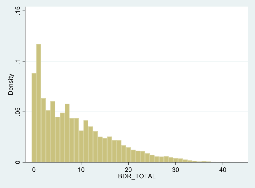
Next, we create the youths (150 in this case, but these numbers can be increased or decreased) and assign them to home locations, which is set based on the size of the grid that represents the world so that randomly sending youth to a home cell results in a combination of both spread (i.e., multiple families are represented) and overlap (i.e., households can have more than one youth). Future iterations of this model can systematically test the effect of youth density, and can allow youth who are randomly sent to the same home cell at initialization to be siblings. Youth, rather than home cells, are assigned their family-risk and family-promotive scores. Similar to the distribution of school and neighborhood risk and prosocial opportunity scores, the family scores are assumed to follow an exponential distribution. This is based on the distribution of actual data from youth on probation from one mid-Atlantic state (Virginia Department of Juvenile Justice 2019), where the family risk subscale appears to follow an exponential distribution as shown in Figure 3. These scores are also restricted to between 0.01 and 0.99, since they act as probabilities in this model. In life, there is always some uncertainty, so actual values of 0 and 1 are not assigned.
Running the model
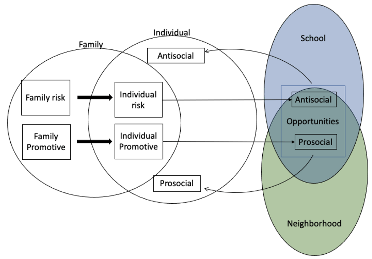
Once the agents and their environment has been created, the model can be run. In the model, each tick represents a day for each youth, since youth are faced with opportunities and make decisions about activities and behaviors every day. The ability to represent a day is a strength of this ABM approach, since prior tests of the theory are based on multiple point-in-time measures separated by months and/or years (Hoffmann et al. 2013; Jang 1999; Lee 2003; Thornberry et al. 1991). Figure 4 shows the conceptual logic of the model while Figure 5 is a flow diagram of the overall model. Figure 5 is laid out similar to the artificial world where the flow at school is in the brown top section, the flow in the neighborhood is in the green middle section, and the flow at home is in the blue bottom section.
While a tick in the model represents 1 day, this is broken into hourly activity increments. The schedule of activities start at the beginning of the day, where the youth goes directly to school and spends 6 hours (7am-2pm) there. This duration is an estimate based on a typical high school day in the United States. At each hour, the youth may be presented with a prosocial opportunity, depending on the probability of a prosocial opportunity assigned to the school location the youth is on. The rationale for this is that these hourly choices roughly approximate students switching classes during the school day and the interactions/exchanges that occur during those transitional periods. If the youth chooses the prosocial opportunity, which is based on their individual promotive score (a probability), they move to a different location in the school. If not, they youth may be presented with an antisocial opportunity, depending on the probability of a risk opportunity assigned to the school location the youth is on. In this model, the antisocial opportunity is leaving school early (i.e., playing hooky). Whether the youth takes the opportunity depends on their individual risk score (a probability).
If the youth stays in school for the whole day, the youth’s tally of prosocial experiences may increase depending on the youth location’s promotive score (i.e., probability of having a lasting positive impact on a student). If the youth leaves school early (i.e., truant), depending on the youth location’s risk opportunity, the youth’s tally of antisocial experiences may increase (i.e., probability of having a lasting negative impact on the student). If the tally increases, whether prosocial or antisocial, it increases in an equal increment – the overall score relative to the other youth in the model is more informative than a single instance of increasing a youth’s tally. This randomness is programmed since it is assumed that every event will not be equally impactful on the youth.
Next, the youth is in the neighborhood for 5 hours (2pm-7pm). This represents the youth’s growing autonomy, which coincides with the growing influence of peers during this period (Stoddard et al. 2012). During this time, the youth may encounter a prosocial influence depending on their location’s promotive score (a probability). If the youth chooses the prosocial opportunity, based on their individual promotive score (a probability), their tally of prosocial experiences will increase. If they do not encounter a prosocial influence, they have a chance of encountering an antisocial influence depending on their location’s risk score (a probability). If the youth chooses the antisocial opportunity, based on their individual risk score (a probability), then their tally of antisocial experiences increases. If the tally increases, whether prosocial or antisocial, it increases in an equal increment – the overall score relative to the other youth in the model is more informative than a single instance of increasing a youth’s tally. This randomness is programmed since it is assumed that every event will not be equally impactful on the youth.
Finally, the youth is at home for 4 hours (7pm-11pm) prior to going to sleep. During this time, the individual risk or promotive score can be modified through their families, who are one of their primary socializing influences (Lee 2014). Youth may be influenced positively or negatively depending on the family risk and promotive scores (Stoddard et al. 2012). Whether the youth is susceptible to the influence is dependent on their own individual scores. If the youth’s risk score is greater, they are susceptible to the antisocial influence. If the youth’s promotive score is greater, they are susceptible to the prosocial influence. This operates as a positive feedback loop. Thornberry (1987) describes the youth’s behavioral trajectory, where the reciprocal nature of interactions reinforce each other, resulting in an increasing likelihood of engagement in crime or alternatively, prosocial behaviors. Once all these activities are done the model tick increments by 1.
Model outputs
The model displays the initial distribution of each individual’s family risk and promotive factors, and the distribution of the risk and promotive score for the school and neighborhood cells (see Figure 1). The distributions displaying the risk scores are in red while the distributions displaying the promotive scores are blue. The distribution of individual risk and promotive scores are shown at initialization and overlaid upon each other, where risk scores are red and promotive scores are blue. The individual risk and promotive scores are updated throughout the model, and when a run has been completed, the final distribution of individual risk and promotive scores are displayed. Additionally, both the average antisocial experience and prosocial experience scores are displayed and updated throughout the simulation, as well as the percent of youth in the simulation with an antisocial score that is higher than their prosocial score. The graph shows the percent of youth with a higher antisocial score (red), higher prosocial score (blue), and equal scores (purple) with each time tick and updates throughout the simulation.
Results
Before presenting the results of the model we first want to discuss efforts we made pertaining to the verification of the model. In order to ensure the model was implemented correctly, verification of the model was conducted throughout the programming of the model – this included code walk throughs to ensure no apparent logical or programming errors were made, and that the model runs as designed (i.e., as shown in Figure 5). This was ascertained through the plots that are displayed in the console (as shown in Figure 1), showing the initial distribution of family, school, and neighborhood risk (red histograms) and promotive (blue histograms) scores. The youth’s individual risk and promotive scores are captured on the same plot, and these are the only scores that change throughout the model.
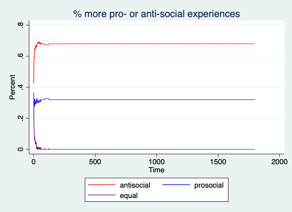
As noted in Section 3.1 we took a stylized facts approach to building this model. While we have risk assessment data for youth in probation, we do not have risk assessment data for the general population. Instead, validation of the model is based on known broad patterns rather than specific details about risk (Heine et al. 2005). The model itself is designed to simulate the clustering of risk, and in this sense, where each new simulation can set different risk levels, each simulation can be thought of as representing different neighborhoods (rather than a single simulation representing multiple neighborhoods). Additionally, both theories of deviance (e.g. Thornberry 1987 interactional theory of delinquency; Sampson & Laub 1997 life course theory of cumulative disadvantage) and empirical studies (e.g., Kirk & Sampson 2013 study that shows youth who were placed in secure detention returned to an alternative educational track) suggest that many youth experience path dependency, where once they begin on either a positive or negative trajectory, it can be difficult to shift trajectories. This is how the model is programmed and operates – in the model, youth seem to stabilize as more antisocial or more prosocial fairly quickly, capturing real life experiences of youth who may find themselves on a negative or positive trajectory, reflecting the difficulty of “switching tracks” once they launch in a certain direction. Figure 6 demonstrates an example model run which shows that youth tend to stabilize as more antisocial (red line) or prosocial (blue line). In this sense, we see elements of level 1 validation, where the model produces qualitative agreement with empirical macrostructures (Axtell & Epstein 1994).
In order to test the sensitivities of the model, we ran simulations, with variables systematically altered, so that there were 10 simulations of 1800 days with each of the six variables (family risk-level, family promotive-level, school risk-level, school promotive-level, neighborhood risk-level, and neighborhood promotive-level) were set at values of .25, .50, and .75 probabilities across a total of 7,290 runs. Generally, each simulation, showed that within about 100 days, the percent of youth who have more antisocial than prosocial experiences seems to stabilize, a representative example of this is shown in Figure 6. Thus, in addition to representing the teen years (approximately five years, from ages 13- 18), 1800 days is more than enough time for each simulation to stabilize.
In order to explore the associations between outcomes and environmental risk and promotive scores we utilize bivariate analyses (analysis of variance) and multivariate analyses (ordinary least squares (OLS) regression) to test for statistical significance. Table 2 shows results from the 7,290 completed simulations. The top panel shows the youth outcomes – the average youth antisocial and prosocial experience scores, as well as the percent of youth classified as antisocial, defined as those with higher antisocial than prosocial scores. The assumption is that a youth whose antisocial experiences outweigh their prosocial experiences will make more antisocial choices, will be more likely to engage in delinquency and crime. The model generates higher antisocial scores, on average, than prosocial scores. Yet, on average, the model generates a fairly even split between youth who are antisocial and youth who are prosocial. The second panel shows average family, school, and neighborhood risk and promotive scores, which were systematically altered. Thus, all six variables with the same mean of .33 confirms that there were an equal number of simulations across the .25, .50, and .75 risk and promotive probabilities in combination with the exponential distribution, which would generate more values at the lower end of the continuum (rather than .50 if the normal distribution had been used).
| Variable | Mean | Std. Dev. | Min | Max |
|---|---|---|---|---|
| Youth Outcome | ||||
| Antisocial Experience Scores | 174.60 | 46.26 | 61.53 | 347.36 |
| Prosocial Experience Scores | 105.94 | 26.25 | 44.98 | 200.95 |
| Percent Antisocial = (antisocial>prosocial) | 0.50 | 0.11 | 0.21 | 0.79 |
| Distributions based on user-controlled probabilities (.25; .50; .75) | ||||
| Family Risk | 0.328 | 0.068 | 0.174 | 0.495 |
| Family Promotive | 0.328 | 0.069 | 0.181 | 0.482 |
| School Risk | 0.328 | 0.068 | 0.189 | 0.469 |
| School Promotive | 0.329 | 0.068 | 0.187 | 0.474 |
| Neighborhood Risk | 0.329 | 0.066 | 0.218 | 0.430 |
| Neighborhood Promotive | 0.329 | 0.066 | 0.219 | 0.424 |
Figures 7, 8, and 9 show bivariate associations between the three outcomes, prosocial experience scores, antisocial experience scores, and percent antisocial, respectively, and the six user-controlled variables (family promotive, family risk, schools promotive, school risk, neighborhood promotive, and neighborhood risk) set at values of .25, .50 and .75. The bivariate associations are significant between prosocial experience score and the family risk and promotive levels. Additionally, the association between prosocial experience score and school and neighborhood promotive level are significant, but not risk level. On the other hand, all six are significantly associated with the antisocial experience score. In terms of the percent who are more antisocial in each model, the family risk and promotive levels are significant, as is the schools promotive score, but not the neighborhood promotive nor the risk score for schools and neighborhood.
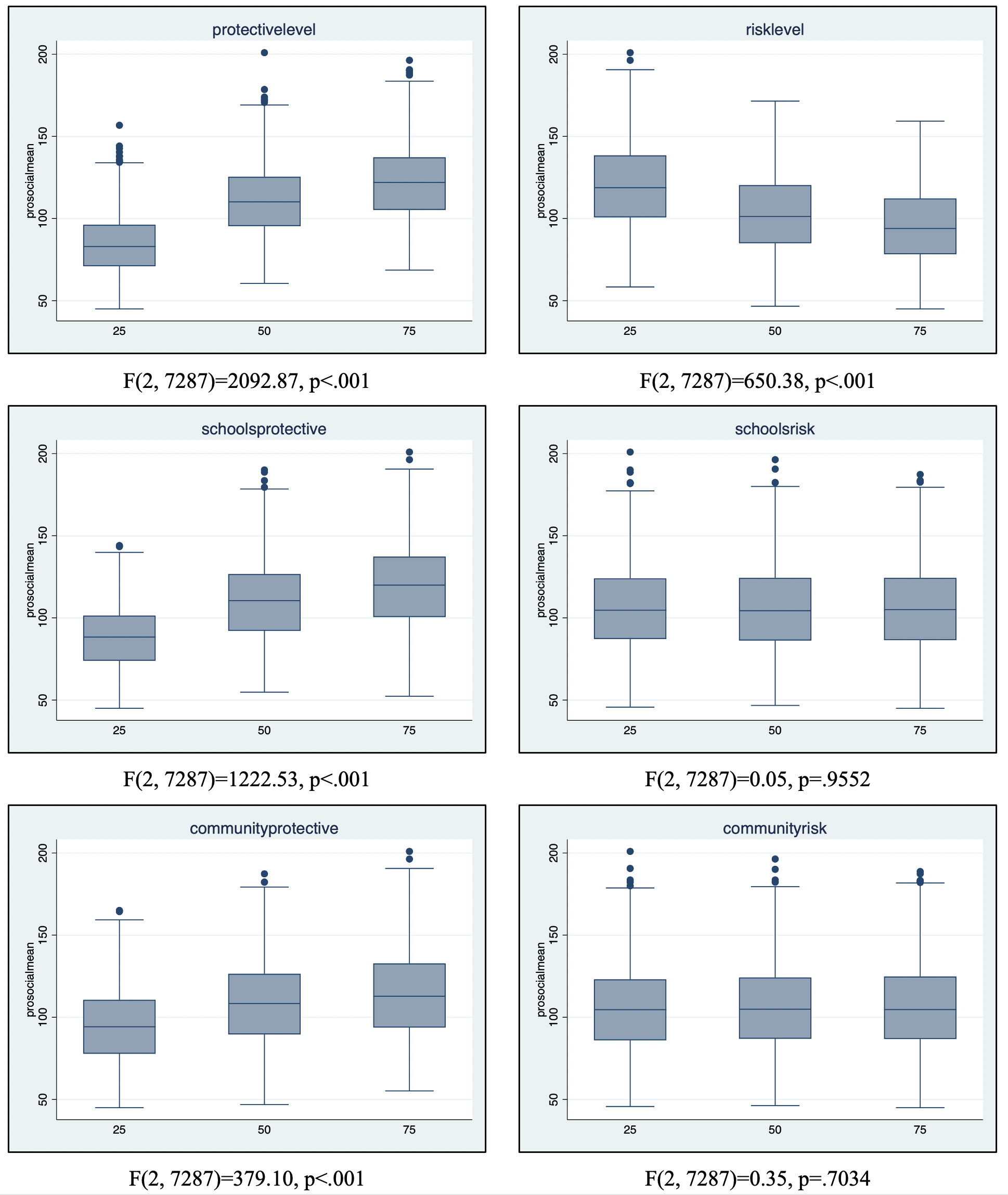
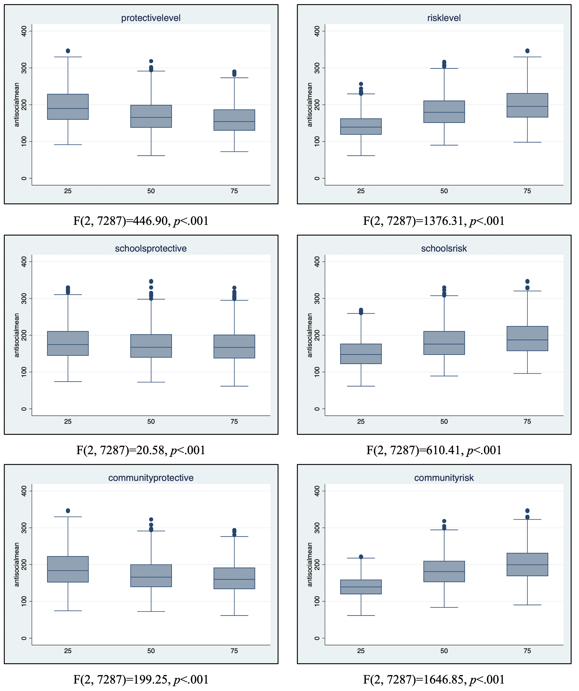
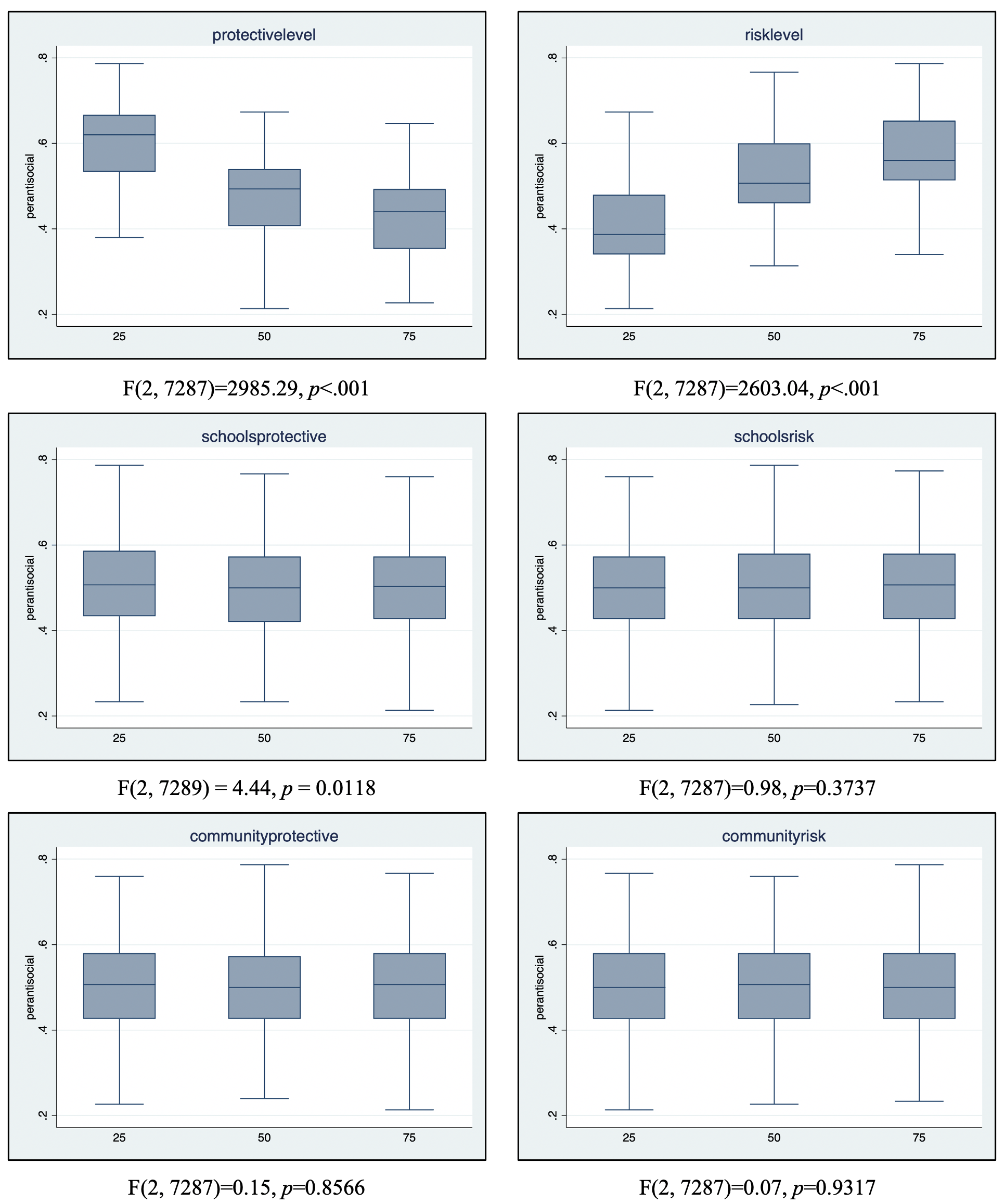
Table 3 presents results from multivariate analyses, which are consistent with the bivariate analyses. The OLS regression models indicate that the six environmental risk and promotive factors (family, school, and neighborhood) are all significantly associated with antisocial experience scores. The prosocial experience scores are significantly associated with the family risk and promotive scores, as well as the promotive scores for schools and neighborhood, but not the risk scores. Finally, the percent antisocial is significantly associated with the family and school risk and promotive scores, but not the neighborhood risk and promotive scores.
We also conducted sensitivity analyses to test whether the results are an artefact of the layout of the model. Reducing the relative size of the neighborhoods (from 75% of the grid to 50% and 25%) and increasing the relative size of the school (from 12.5% of the grid to 37.5% and 62.5% ) results in a new statistically significant coefficient in the OLS model – school risk was statistically significant in the prosocial experiences regression model. Also, a surprising change was that while the size of the neighborhood decreased, neighborhood risk became statistically significant in the percent antisocial regression model. Yet, the non significance of neighborhood risk on prosocial experiences and neighborhood promotive on percent antisocial remained robust. Additionally, it is more likely that a youth’s neighborhood will be larger than their school neighbourhoods, so we focus the remainder of our discussion on the default configuration of the model. Readers, who wish to explore this in more detail, can do so by downloading the model from https://bit.ly/YaTASERPS.
| Antisocial Experience Scores | Prosocial Experience Scores | Percent Antisocial | ||||||||||
| B | Std B | SE | p | B | Std B | SE | p | B | Std B | SE | p | |
| Family Risk | 372.05 | 0.550 | 1.85 | *** | -158.88 | -0.414 | 1.13 | *** | 1.10 | 0.679 | 0.004 | *** |
| Family Promotive | -231.98 | -0.345 | 1.83 | *** | 241.82 | 0.635 | 1.12 | *** | -1.13 | -0.703 | 0.004 | *** |
| Schools Risk | 267.64 | 0.394 | 1.85 | *** | -1.44 | -0.004 | 1.13 | 0.03 | 0.021 | 0.004 | *** | |
| Schools Promotive | -52.23 | -0.077 | 1.86 | *** | 202.00 | 0.524 | 1.14 | *** | -0.05 | -0.032 | 0.004 | *** |
| Neighborhood Risk | 393.43 | 0.560 | 1.92 | *** | 1.42 | 0.004 | 1.17 | 0.01 | 0.004 | 0.005 | ||
| Neighborhood Promotive | -161.35 | -0.229 | 1.92 | *** | 123.77 | 0.310 | 1.18 | *** | 0.00 | -0.002 | 0.005 | |
| Constant | -18.41 | . | 1.51 | *** | -28.45 | . | 0.92 | *** | 0.52 | . | 0.004 | *** |
| R2 | 0.95 | 0.94 | 0.95 | |||||||||
Summary
While risk assessments are widely used within criminal and juvenile justice systems to inform sanctions and interventions, within this paper we have argued that these risk assessments tend to focus on individual risk and often fail to capture each individual’s environmental risk (see Section 2.2). In order to address this failure, within this paper we have presented an agent-based model that explores the interaction of individual and environmental risk on the youth based on the interactional theory of delinquency (Thornberry 1987; Thornberry et al. 1991; Thornberry & Krohn 2005). By focusing on the dynamics and processes that evolve from interactions between agents (i.e., youths) and their environments, this model is a first step beyond more traditional statistical approaches used to study delinquency that tend to rely on point-in-time measures.
The model presented in this paper provides preliminary support for how environmental risk and promotive factors may play an important role in shaping youth outcomes and that the family risk and promotive levels appear to be related to both individual antisocial and prosocial experience scores. Results from the model (Section 4) show how the family can play an important role in the lives of youth, which suggests that increasing the family’s promotive factors while reducing the family’s risk factors may be an effective way to induce lasting impacts on youth outcomes. Such a finding may suggest that practitioners should consider family service needs (e.g., household poverty, parental mental illness, and parental substance use issues) in order to reduce family risk.
In contrast, only the promotive factors in the neighborhoods and schools, and not risk factors, are related to prosocial outcomes within the model. This may reflect the distinct processes that operate within the real world, and may emphasize that increasing promotive factors may be more important than simply reducing risk. In fact, the non significant association between neighborhood risk and prosocial experiences was very robust to our sensitivity analyses. Opportunities for students to become involved in positive activities, such as theater or sports after school, may effectively reduce delinquency while also contributing to the positive social development of the youth. Further, when considering both antisocial in conjunction with prosocial experiences, where a youth was classified as “antisocial” if their overall antisocial experiences were greater than their overall prosocial experiences, the model showed that the family risk and promotive levels continued to be significant. However, the school promotive level, but not the other environmental settings (i.e., schools risk, neighborhood promotive, neighborhood risk) were found to be significant. This is in line with Hoffmann et al. (2013) finding that academic achievement was important for reducing delinquency.
As with all modeling endeavors, there are limitations with the model presented in this paper and additional factors could always be added to any model, this is one reason we provide the code and a detailed description of the model (see Section 3.2), which allows others to extend the model if they so desire. Even though the model enriches our understanding of how risk and promotive factors are generated, and how youth experience both prosocial and antisocial socialization processes, we will now discuss some logical next steps.
For example, while developing this agent-based model based on Thornberry (1987) interactional theory of delinquency, it underscores not only the issue of taking theory and implementing it in code, but also highlights the limits of our current understanding of risk and promotive factors. In our case, we recognized the lack of knowledge of generative mechanisms of risk since modeling requires explicitly identifying the mechanisms that generate existing patterns. While it is well accepted that more risk factors translate into a higher likelihood of delinquency (Appleyard et al. 2005; Baglivio et al. 2017; Farrington et al. 2016), it is unclear how risk accumulates, and how risk operates. Within this paper we made assumptions about how existing risk is generated and operate, but these assumptions could also be explicitly tested in the future by collecting empirical data that can be used to provide additional validation of this model. Thus, the model offers opportunities for deepening our understanding of how risk is generated and how risk operates.
Another area for further work is how and when antisocial and prosocial experiences accumulate. In our model, we made the assumption that these were additive (i.e., linear). In the sense, that if a youth leaves school early, their antisocial experience score increases, while if they stay in school, their prosocial experience score increases. If while in the neighborhood, they engage with the negative influence, their antisocial experience score increases, and if they engage with a positive influence, their prosocial experience score increases. Finally, depending on both the family’s risk and promotive factors, and the individual’s risk in comparison to promotive factor, the youth’s individual risk or promotive factor score may increase. This is assumed to reflect a model of accumulating advantage and accumulating disadvantage, where those with a higher risk score might experience additive increases in their risk score, and those with higher promotive scores might experience additive increases in their promotive scores. The linear nature of these associations should be tested in future work, for example, perhaps it is not a linear accumulation, but rather, some sort of association that reflects diminishing returns over time.
Finally, two distinct processes, one antisocial and one prosocial, are assumed. In this model, there is little interaction between the risk and promotive scales, and little interaction between the antisocial and prosocial experience scores. While there is some empirical evidence to support this assumption (e.g., Hoge et al., 1996), this is not a well-accepted approach to delinquency since researchers focus primarily on predicting delinquency and recidivism. This is one of the benefits of agent-based modeling (Epstein, 2008), to test assumptions, and therefore help inform this debate through simulation. Even though there are many areas of possible future work, the model presented in this paper allows us a means of estimating risk and promotive scores for environments and observing how youth may interact with their environments to simulate prosocial and antisocial development from the bottom up. Not only does this help improve our understanding of delinquency at the individual level but demonstrates how agent-based models can be used within the field of social work and thus helps open up new areas of research that promote wellbeing of societies.
Model Documentation
The model itself was created in NetLogo version 6.1.0 (Wilensky 1999) and a detailed Overview, Design concepts, and Details plus Decision (ODD + D) protocol (Müller et al. 2013) document, which extends the ODD protocol (Grimm et al. 2006) is available at: https://bit.ly/YaTASERPS. We provide this documentation in order to provide more details about the model and aid others in replicating the results presented in this paper along with extending the model if so desired.References
ABRAM, K. M., Azores-Gococo, N. M., Emanuel, K. M., Aaby, D. A., Welty, L. J., Hershfield, J. A., Rosenbaum, M. S., & Teplin, L. A. (2017). Sex and racial/ethnic differences in positive outcomes in delinquent youth after detention: A 12-Year longitudinal study. JAMA Pediatrics, 171(2), 123. [doi:10.1001/jamapediatrics.2016.3260]
ABRAM, K. M., Teplin, L. A., McClelland, G. M., & Dulcan, M. K. (2003). Comorbid psychiatric disorders in youth in juvenile detention. Archives of General Psychiatry, 60(11), 1097–1108. [doi:10.1001/archpsyc.60.11.1097]
AGNEW, R. (2003). An integrated theory of the adolescent peak in offending. Youth and Society, 34(3), 263–299. [doi:10.1177/0044118x02250094]
APPLEYARD, K., Egeland, B., Dulmen, M. H. M., & Alan Sroufe, L. (2005). When more is not better: The role of cumulative risk in child behavior outcomes. Journal of Child Psychology and Psychiatry, 46(3), 235–245. [doi:10.1111/j.1469-7610.2004.00351.x]
ARTHUR, M. W., Hawkins, J. D., Pollard, J. A., Catalano, R. F., & Baglioni Jr., A. J. (2002). Measuring risk and protective factors for substance use, delinquency, and other adolescent problem behaviors: The communities that care youth survey. Evaluation Review, 26(6), 575–601. [doi:10.1177/019384102237850]
AXELROD, R. (1997). 'Advancing the art of simulation in the social sciences.' In R. Conte, R. Hegselmann, &amamp; P. Terna (Eds.), Simulating Social Phenomena (pp. 21–40). Berlin, Heidelberg: Springer.
AXTELL, R., & Epstein, J. M. (1994). Agent-Based modelling: Understanding our creations. The Bulletin of the Santa Fe Institute, 9(4), 28–32.
BAGLIVIO, M. T. (2009). The assessment of risk to recidivate among a juvenile offending population. Journal of Criminal Justice, 37(6), 596–607. [doi:10.1016/j.jcrimjus.2009.09.008]
BAGLIVIO, M. T., Epps, N., Swartz, K., Huq, M. S., Sheer, A., & Hardt, N. S. (2014). The prevalence of adverse childhood experiences (ACE) in the lives of juvenile offenders. Journal of Juvenile Justice, 3(2), 1–23. [doi:10.1037/e529382014-012]
BAGLIVIO, M. T., Wolff, K. T., Piquero, A. R., Howell, J. C., & Greenwald, M. A. (2017). Risk assessment trajectories of youth during juvenile justice residential placement: Examining risk, promotive, and “Buffer” scores. Criminal Justice and Behavior, 44(3), 360–394. [doi:10.1177/0093854816668918]
BAIRD, C., Healy, T., Johnson, K., Bogie, A., Dankert, E. W., & Scharenbroch, C. (2013). A comparison of risk assessment instruments in juvenile justice. Madison, WI: National Council on Crime and Delinquency.
BARNERT, E. S., Abrams, L. S., Dudovitz, R., Coker, T. R., Bath, E., Tesema, L., Nelson, B. B., Biely, C., & Chung, P. J. (2019). What is the relationship between incarceration of children and adult health outcomes? Academic Pediatrics, 19(3), 342–350. [doi:10.1016/j.acap.2018.06.005]
BOYLE, S., Guerin, S., Pratt, J., & Kunkle, D. (2003). Application of agent-based simulation to policy appraisal in the criminal justice system in England and Wales. In C. M. Macal, M. J. North, & D. Sallach (Eds.), Proceedings of Agent 2003 Conference on Challenges in Social Simulation (pp. 493–507). [doi:10.4018/978-1-59140-649-5.ch012]
BRUMLEY, L. D., & Jaffee, S. R. (2016). Defining and distinguishing promotive and protective effects for childhood externalizing psychopathology: A systematic review. Social Psychiatry and Psychiatric Epidemiology, 51(6), 803–815. [doi:10.1007/s00127-016-1228-1]
ELDER, G. H. (1994). Time, human agency, and social change: Perspectives on the life course. Social Psychology Quarterly, 57(1), 4–15.
FARRINGTON, D. P. (2015). Prospective longitudinal research on the development of offending. Australian & New Zealand Journal of Criminology, 48(3), 314–335. [doi:10.1177/0004865815590461]
FARRINGTON, D. P., Ttofi, M. M., & Piquero, A. R. (2016). Risk, promotive, and protective factors in youth offending: Results from the Cambridge study in delinquent development. Journal of Criminal Justice, 45(s), 63–70. [doi:10.1016/j.jcrimjus.2016.02.014]
GARAVAGLIA, C., Malerba, F., Orsenigo, L., & Pezzoni, M. (2013). A simulation model of the evolution of the pharmaceutical industry: A history-friendly model. Journal of Artificial Societies and Social Simulation, 16(4), 5: https://www.jasss.org/16/4/5.html. [doi:10.18564/jasss.2314]
GILBERT, N., Ahrweiler, P., Barbrook-Johnson, P., Narasimhan, K., & Wilkinson, H. (2018). Computational modelling of public policy: Reflections on practice. Journal of Artificial Societies and Social Simulation, 21(1), 14: https://www.jasss.org/21/1/14.html [doi:10.18564/jasss.3669]
GILBERT, N., & Troitzsch, K. G. (2005). Simulation for the Social Sciences. Milton Keynes: Open University Press.
GOTTFREDSON, M., & Hirschi, T. (1987). The methodological adequacy of longitudinal research on crime. Criminology, 25(3), 581–614. [doi:10.1111/j.1745-9125.1987.tb00812.x]
GOTTFREDSON, M. R., & Hirschi, T. (1990). A General Theory of Crime. Palo Alto, CA: Stanford University Press.
GRIMM, V. (2002). Visual debugging: A way of analyzing, understanding and communicating bottom-up simulation models in ecology. Natural Resource Modeling, 15(1), 23–38. [doi:10.1111/j.1939-7445.2002.tb00078.x]
GRIMM, V., Berger, U., Bastiansen, F., Eliassen, S., Ginot, V., Giske, J., Goss-Custard, J., Grand, T., Heinz, S., Huse, G., Huth, A., Jepsen, J., Jorgensen, C., Mooij, W., Muller, B., Pe’er, G., Piou, C., Railsback, S., Robbins, A., … Deangelis, D. (2006). A standard protocol for describing individual-Based and agent-Based models. Ecological Modelling, 198(1–2), 115–126. [doi:10.1016/j.ecolmodel.2006.04.023]
GROFF, E. R. (2007). Simulation for theory testing and experimentation: An example using routine activity theory and street robbery. Journal of Quantitative Criminology, 23(2), 75–103. [doi:10.1007/s10940-006-9021-z]
GRUNWALD, H. E., Lockwood, B., Harris, P. W., & Mennis, J. (2010). Influences of neighborhood context, individual history and parenting behavior on recidivism among juvenile offenders. Journal of Youth and Adolescence, 39(9), 1067–1079. [doi:10.1007/s10964-010-9518-5]
HARRIS, P. W., Mennis, J., Obradovic, Z., Izenman, A. J., & Grunwald, H. E. (2011). The coaction of neighborhood and individual effects on juvenile recidivism. Cityscape: A Journal of Policy Development and Research, 13(3), 33–55.
HAZEL, N. (2008). Cross-national comparison of youth justice. London: Youth Justice Board for England and Wales. Available at: https://dera.ioe.ac.uk/7996/1/Cross_national_final.pdf
HEINE, B. O., Meyer, M., & Strangfeld, O. (2005). Stylised facts and the contribution of simulation to the economic analysis of budgeting. Journal of Artificial Societies and Social Simulation, 8(4), 4: https://www.jasss.org/8/4/4.html.
HIANCE, D., Doogan, N., Warren, K., Hamilton, I. M., & Lewis, M. (2012). An agent-based model of lifetime attendance and self-help program growth. Journal of Social Work Practice in the Addictions, 12(2), 121–142. [doi:10.1080/1533256x.2012.669702]
HILTERMAN, E. L. B., Nicholls, T. L., & van Nieuwenhuizen, C. (2014). Predictive validity of risk assessments in juvenile offenders: Comparing the SAVRY, PCL: YV, and YLS/CMI with unstructured clinical assessments. Assessment, 21(3), 324–339. [doi:10.1177/1073191113498113]
HOFFMANN, J. P., Erickson, L. D., & Spence, K. R. (2013). Modeling the association between academic achievement and delinquency: An application of interactional theory. Criminology, 51(3), 629–660. [doi:10.1111/1745-9125.12014]
HOGE, R. D., Andrews, D. A., & Leschied, A. W. (1996). An investigation of risk and protective factors in a sample of youthful offenders. Journal of Child Psychology and Psychiatry, 37(4), 419–424. [doi:10.1111/j.1469-7610.1996.tb01422.x]
IHARA, E. S., & Lee, J. S. (2019). Agent-Based modeling: Value added to social work research. Families in Society, 100(3), 305–311. [doi:10.1177/1044389419842764]
ISRAEL, N., & Wolf-Branigin, M. (2011). Nonlinearity in social service evaluation: A primer on agent-based modeling. Social Work Research, 35(1), 20–24. [doi:10.1093/swr/35.1.20]
JACOBY, J. E., Severance, T. A., & Bruce, A. S. (Eds.). (2004). Classics of Criminology. Prospect Heights, IL: Waveland Press.
JANG, S. J. (1999). Age-varying effects of family, school, and peers on delinquency: A multilevel modeling test of interactional theory. Criminology, 37(3), 643–686. [doi:10.1111/j.1745-9125.1999.tb00499.x]
JONES, N. J., Brown, S. L., Robinson, D., & Frey, D. (2016). Validity of the youth assessment and screening instrument: A juvenile justice tool incorporating risks, needs, and strengths. Law and Human Behavior, 40(2), 182–194. [doi:10.1037/lhb0000170]
KENNEDY, W. G., Ihara, E. S., Tompkins, C. J., & Wolf-Branigin, M. E. (2015). Computational modeling of caregiver stress. Journal of Policy Studies and Complex Systems, 2(1), 31–44. [doi:10.18278/jpcs.2.1.5]
KIRK, D. S., & Sampson, R. J. (2013). Juvenile arrest and collateral educational damage in the transition to adulthood. Sociology of Education, 86(1), 36–62. [doi:10.1177/0038040712448862]
LANGELLIER, B. A., Yang, Y., Purtle, J., Nelson, K. L., Stankov, I., & Roux, A. V. D. (2019). Complex systems approaches to understand drivers of mental health and inform mental health policy: A systematic review. Administration and Policy in Mental Health and Mental Health Services Research, 46(2), 128–144. [doi:10.1007/s10488-018-0887-5]
LEAW, J. N., Ang, R. P., Huan, V. S., Chan, W. T., & Cheong, S. A. (2015). Re-examining of Moffitt’s theory of delinquency through agent based modeling. PlOS ONE, 10, e0126752. [doi:10.1371/journal.pone.0126752]
LEE, J. S. (2014). An institutional framework for the study of the transition to adulthood. Youth and Society, 46(5), 706–730. [doi:10.1177/0044118x12450643]
LEE, J. S., & Ballew, K. M. (2018). Independent living services, adjudication status, and the social exclusion of foster youth aging out of care in the United States. Journal of Youth Studies, 21(7), 940–957. [doi:10.1080/13676261.2018.1435854]
LEE, J. S., & Taxman, F. S. (2020). Using latent class analysis to identify the complex needs of youth on probation. Children and Youth Services Review, 115, 105087. [doi:10.1016/j.childyouth.2020.105087]
LEE, J. S., & Wolf-Branigin, M. (2020). Innovations in modeling social good: A demonstration with juvenile justice intervention. Research on Social Work Practice, 30(2), 174–185. [doi:10.1177/1049731519852151]
LEE, S. (2003). Testing Thornberry’s interactional theory: The reciprocal relations. Iowa State University, PhD Thesis. [doi:10.31274/rtd-180817-80]
LOEBER, R., & Le Blanc, M. (1990). Toward a developmental criminology. Crime and Justice, 12, 375–473. [doi:10.1086/449169]
MALLESON, N., Heppenstall, A., See, L., & Evans, A. (2013). Using an agent-based crime simulation to predict the effects of urban regeneration on individual household burglary risk. Environment and Planning B: Planning and Design, 40(3), 405–426. [doi:10.1068/b38057]
MASCHI, T., Hatcher, S. S., Schwalbe, C. S., & Rosato, N. S. (2008). Mapping the social service pathways of youth to and through the juvenile justice system: A comprehensive review. Children and Youth Services Review, 30(12), 1376–1385. [doi:10.1016/j.childyouth.2008.04.006]
MEYER, M. (2011). Bibliometrics, stylized facts and the way ahead: How to build good social simulation models of science? Journal of Artificial Societies and Social Simulation, 14(4), 4: https://www.jasss.org/14/4/4.html. [doi:10.18564/jasss.1824]
MOFFITT, T. E. (1993). Adolescence-limited and life-course-persistent antisocial behavior: A developmental taxonomy. Psychological Review, 100(4), 674–701. [doi:10.1037/0033-295x.100.4.674]
MÜLLER, B., Bohn, F., Dreßler, G., Groeneveld, J., Klassert, C., Martin, R., Schlüter, M., Schulze, J., Weise, H., & Schwarz, N. (2013). Describing human decisions in agent-Based models ODD + D, An extension of the ODD protocol. Environmental Modelling & Software, 48, 37–48.
OH, H., Trinh, M. P., Vang, C., & Becerra, D. (2020). Addressing barriers to primary care access for Latinos in the US: An agent-Based model. Journal of the Society for Social Work and Research, 11(2), 165–184. [doi:10.1086/708616]
ONIFADE, E., Davidson, W., Livsey, S., Turke, G., Horton, C., Malinowski, J., Atkinson, D., & Wimberly, D. (2008). Risk assessment: Identifying patterns of risk in young offenders with the Youth Level of Service/Case Management Inventory. Journal of Criminal Justice, 36(2), 165–173. [doi:10.1016/j.jcrimjus.2008.02.006]
PETERSON-BADALI, M., Skilling, T., & Haqanee, Z. (2015). Examining implementation of risk assessment in case management for youth in the justice system. Criminal Justice and Behavior, 42(3), 304–320. [doi:10.1177/0093854814549595]
RODRIGUEZ, N. (2013). Concentrated disadvantage and the incarceration of youth: Examining how context affects juvenile justice. Journal of Research in Crime and Delinquency, 50(2), 189–215. [doi:10.1177/0022427811425538]
SAMPSON, R. J., & Laub, J. H. (1997). 'A life-course theory of cumulative disadvantage and the stability of delinquency.' In T. P. Thornberry (Ed.), Developmental theories of crime and delinquency (pp. 133–161). Transaction Publishers.
SAMPSON, R. J., Morenoff, J. D., & Gannon-Rowley, T. (2002). Asessing "neighborhood effects": Social processes and new directions in research. Annual Review of Sociology, 28(1), 443–478. [doi:10.1146/annurev.soc.28.110601.141114]
SCHUHMACHER, N., Ballato, L., & van Geert, P. (2014). Using an agent-based model to simulate the development of risk behaviors during adolescence. Journal of Artificial Societies and Social Simulation, 17(3), 1: https://www.jasss.org/17/3/1.html. [doi:10.18564/jasss.2485]
SCHWALBE, C. S., Macy, R. J., Day, S. H., & Fraser, M. W. (2008). Classifying offenders: An application of latent class analysis to needs assessment in juvenile justice. Youth Violence and Juvenile Justice, 6(3), 279–294. [doi:10.1177/1541204007313383]
SERIN, R. C., Chadwick, N., & Lloyd, C. D. (2016). Dynamic risk and protective factors. Psychology, Crime & Law, 22(1–2), 151–170. [doi:10.1080/1068316x.2015.1112013]
SIMON, H. A. (1996). The Sciences of the Artificial. Cambridge, MA: MIT Press.
SLOBOGIN, C. (2012). Risk assessment and risk management in juvenile justice. Criminal Justice, 27(4), 10–25.
STODDARD, S. A., Zimmerman, M. A., & Bauermeister, J. A. (2012). A longitudinal analysis of cumulative risks, cumulative promotive factors, and adolescent violent behavior. Journal of Research on Adolescence, 22(3), 542–555. [doi:10.1111/j.1532-7795.2012.00786.x]
SUTHERLAND, E. H. (1947). Principles of Criminology. Chicago, IL: J. J.B. Lippincott.
TAXMAN, F. S., & Caudy, M. S. (2015). Risk tells us who, but not what or how: Empirical assessment of the complexity of criminogenic needs to inform correctional programming. Criminology & Public Policy, 14(1), 71–103. [doi:10.1111/1745-9133.12116]
TEPLIN, L. A., Abram, K. M., McClelland, G. M., Dulcan, M. K., & Mericle, A. A. (2002). Psychiatric disorders in youth in juvenile detention. Archives of General Psychiatry, 59, 1133–1143. [doi:10.1001/archpsyc.59.12.1133]
TESFATSION, L., & Judd, K. L. (2006). Handbook of Computational Economics: Agent-Based Computational Economics. Amsterdam: North-Holland Publishing.
THORNBERRY, T. P. (1987). Toward an interactional theory of delinquency. Criminology, 25(4), 863–892. [doi:10.1111/j.1745-9125.1987.tb00823.x]
THORNBERRY, T. P., & Krohn, M. D. (2005). 'Applying interactional theory to the explanation of continuity and change in antisocial behavior.' In D. P. Farrington (Ed.), Integrated Developmental and Life-Course Theories of Offending (pp. 183–210). New Brunswick, NJ: Transaction Publishers. [doi:10.4324/9780203788431-8]
THORNBERRY, T. P., Lizotte, A. J., Krohn, M. D., Farnworth, M., & Jang, S. J. (1991). Testing interactional theory: An examination of reciprocal causal relationships among family, school, and delinquency. The Journal of Criminal Law and Criminology, 82(1), 3–35.
VIRGINIA Department of Juvenile Justice. (2019). Data resource guide fiscal year 2019.
WILENSKY, U. (1999). NetLogo. Evanston, IL: Center for Connected Learning and Computer-Based Modeling, Northwestern University.
WRIGHT, K., Muddle, A., Rountree, M., & Rich, E. (2019). Balancing punitive and rehabilitative approaches to juvenile justice: An investigation into the common mechanisms used by countries to prosecute young offenders as adults. Macquarie University, Sydney, Australia.